Microhydrodynamics of an autophoretic particle near a plane interface

Abstract

We study the autophoretic motion of a spherical active particle interacting chemically and hydrodynamically with its fluctuating environment in the limit of rapid diffusion and slow viscous flow. Then, the chemical and hydrodynamic fields can be expressed in terms of integrals over boundaries. The resulting boundary-domain integral equations provide a direct way of obtaining the traction on the particle, requiring the solution of linear integral equations. An exact solution for the chemical and hydrodynamic problems is obtained for a particle in an unbounded domain. For motion near boundaries, we provide corrections to the unbounded solutions in terms of chemical and hydrodynamic Green’s functions, preserving the dissipative nature of autophoresis in a viscous fluid for all physical configurations. Using this, we give the fully stochastic update equations for the Brownian trajectory of an autophoretic particle in a complex environment. Finally, we demonstrate our method by studying autophoresis near a plane interface of fixed viscosity ratio and solute permeability. We provide explicit solutions to the chemical and hydrodynamic problems with high accuracy for this system geometry. We apply our theoretical results in numerical simulations of the dynamics of a bottom-heavy Brownian Janus particle near a wall.

I Introduction

The microhydrodynamics of autophoretic particles comprises particle propulsion by self-generated gradients on their surfaces (Anderson, 1989; Paxton et al., 2006; Moran and Posner, 2017; Ebbens and Howse, 2010) and thermally-induced particle Brownian motion (Batchelor, 1976; Graham, 2018). Autonomous motion without external forces or torques allows autophoretic particles to mimic the locomotion of microorganisms (Goldstein, 2015; Brennen and Winet, 1977), making them useful in the study of the fundamental principles of motility and collective behaviour (Palacci et al., 2013; Illien et al., 2017; Shaebani et al., 2020; Thutupalli et al., 2018; Kumar et al., 2023; Zöttl and Stark, 2023). In particular, the study of autophoresis near surfaces is a focal point due to its relevance in microfluidics, biophysics and surface science (Palacci et al., 2013; Kreuter et al., 2013; Uspal et al., 2015; Ibrahim and Liverpool, 2015; Shen et al., 2018; Singh et al., 2019; Thutupalli et al., 2018). Brownian motion, introducing stochasticity to particle behaviour, can be seen as a diffusive process with a diffusion coefficient that is uniquely linked to the mobility connecting particle motion and forces, a concept that originated from Einstein’s early work (Einstein, 1905) and has since been studied extensively for suspensions of colloidal particles (Zwanzig, 1964; Chow, 1973; Hinch, 1975; Ermak and McCammon, 1978; Ladd, 1994; Cichocki et al., 2000; Keaveny, 2014; Delmotte and Keaveny, 2015; Singh and Adhikari, 2017; Elfring and Brady, 2022; Turk et al., 2022; Bao et al., 2018; Westwood et al., 2022). It is thus of theoretical interest to devise a self-consistent method to explore the interplay of activity-induced autophoresis and configuration-dependent diffusive stresses in the fluid arising from the hydrodynamic coupling of the particle to its thermally fluctuating environment.

Here, we construct a microscopic theory for spherical self-diffusiophoretic particles (propulsion by self-generated chemical concentration gradients) in a fluctuating environment. Chemical gradients generated by the particle induce an osmotic pressure, which is balanced by viscous stresses driving an effective slip flow $\boldsymbol{v}^{\mathcal{A}}$ confined to a thin layer at the surface of the particle (Anderson et al., 1982; Anderson, 1989). The particle thus sets the surrounding fluid in motion, which then reacts back on the particle, creating surface stresses and eventually self-propulsion. In the limit of rapid diffusion and slow viscous flow, the chemical and hydrodynamic fields can be expressed in terms of boundary-domain integrals corresponding to Laplace and Stokes equation, respectively (Singh et al., 2019; Singh and Adhikari, 2017). The boundary integral approach obviates the need to solve for the concentration field and the fluid flow in the bulk, subsequently matching boundary conditions (Golestanian et al., 2005, 2007). Instead, we directly obtain the concentration and the resulting traction (force per unit area) on the surface of the particle. Furthermore, compared to the kinematic squirmer model approach to active particles (Lighthill, 1952; Blake, 1971; Pak and Lauga, 2014), it is straightforward to incorporate in the governing equations the thermal fluctuations of the fluid, which manifest themselves as fluctuating stresses on the particle.

We simultaneously solve the boundary-domain integral equations for the chemical and hydrodynamic fields in a basis of tensor spherical harmonics (TSH). In this basis, we show that the full chemo-hydrodynamic problem of a particle far away from boundaries can be solved exactly (Turk et al., 2022). For motion near boundaries, we provide corrections to the unbounded solutions in terms of chemical and hydrodynamic Green’s functions. The particle’s surface composition influences its generation of slip and is commonly modelled by a phoretic mobility $\mu_{c}$ (Golestanian et al., 2007). Here, we systematically consider non-uniform surfaces, which we confirm can lead to phoretic self-rotation even in the absence of boundaries (Lisicki et al., 2018). Complementing previous work on active particles discretised in a basis of TSH (Ghose and Adhikari, 2014), we define a coupling of slip modes naturally arising from phoretic activity. We give the fully stochastic update equations for the Brownian trajectory of an autophoretic particle in a complex environment in terms of its mobilities and so-called propulsion tensors. The latter are needed only for active particles with slip boundary conditions (Singh et al., 2015). Finally, we demonstrate our method by studying autophoresis near a plane interface of fixed viscosity ratio and solute permeability, extending on some previous works on phoretic self-propulsion near a no-slip wall that is impermeable to solutes (Ibrahim and Liverpool, 2015; Uspal et al., 2015; Shen et al., 2018; Singh et al., 2019). We provide useful explicit one-body solutions to the chemical and hydrodynamic problems to high accuracy, facilitating Brownian simulations with a diffusion matrix that is guaranteed to be positive definite for all physical configurations. This adds to the existing literature on particle mobility (Brenner, 1961; Goldman et al., 1967a; Felderhof, 1976; Perkins and Jones, 1990, 1992; Lee et al., 1979; Lee and Leal, 1980; Swan and Brady, 2007; Daddi-Moussa-Ider et al., 2018) and diffusion (Wajnryb et al., 2004; Rogers et al., 2012; Delong et al., 2015; Lisicki et al., 2016; Ermak and McCammon, 1978) near a boundary and helps in consolidating the idea of propulsion tensors in the same light as mobility matrices for active particles. Finally, we provide Brownian simulations of the fully analytical description above for the special case of a bottom-heavy Janus particle near a wall. Gradually increasing the accuracy with which its dynamics are considered, we investigate the full fluctuating chemo-hydrodynamic effects of the wall on the motion of the particle.

The rest of the paper is organised as follows. In Section II, we review the chemo-hydrodynamic problem of autophoresis in a fluctuating environment and its formal solution via the boundary-domain integral representation of Laplace and Stokes equations. In Section III, we discretise this formal solution in the basis of TSH, finding an exact and an approximate solution to the full chemo-hydrodynamic problem far away from and near boundaries, respectively. We provide the stochastic update equations for thermally-agitated autophoresis in complex environments. Finally, in Section IV, we study the concrete example of a bottom-heavy Brownian Janus particle in the vicinity of a plane interface. We obtain explicit forms of the chemical coupling tensors, the mobility matrices, and the propulsion tensors in this experimentally realisable setting and demonstrate our analytical results by numerical simulations. We conclude with a brief discussion of our results and potential future applications thereof in Section V.

II chemo-hydrodynamics

Chemical problem	Hydrodynamic problem
$\qquad\boldsymbol{\nabla}\cdot\boldsymbol{j}=0$ (Ia)	$\qquad\boldsymbol{\nabla}\cdot\boldsymbol{\sigma}+\boldsymbol{\xi}=0$ (Id)
$\qquad\boldsymbol{j}=-D\boldsymbol{\nabla}c$ (Ib)	$\qquad\boldsymbol{\sigma}=-p\boldsymbol{I}+\eta\left(\boldsymbol{\nabla}\boldsymbol{v}+\left(\boldsymbol{\nabla}\boldsymbol{v}\right)^{\text{tr}}\right)$ (Ie)
$\qquad\boldsymbol{j}(\boldsymbol{R}+\boldsymbol{b})\cdot\hat{\boldsymbol{b}}=j^{\mathcal{A}}(\boldsymbol{b})\qquad$(specified) (Ic)	$\qquad\boldsymbol{v}(\boldsymbol{R}+\boldsymbol{b})=\boldsymbol{v}^{\mathcal{D}}(\boldsymbol{b})+\boldsymbol{v}^{\mathcal{A}}(\boldsymbol{b})$ (If)
Chemo-hydrodynamic coupling:    $\boldsymbol{v}^{\mathcal{A}}(\boldsymbol{b})=\boldsymbol{\chi}\left[c\right],$$\qquad\boldsymbol{\chi}=\mu_{c}(\boldsymbol{b})\big{(}\boldsymbol{I}-\hat{\boldsymbol{b}}\hat{\boldsymbol{b}}\big{)}\cdot\boldsymbol{\nabla}$ (Ig)

Table 1: Governing differential laws. This table summarises the chemo-hydrodynamic coupling at the surface of an autophoretic particle, an example of two three-dimensional partial differential equations, namely Laplace equation for the concentration field (Ia) and Stokes equation for the fluid flow and pressure in a fluid with thermal force $\boldsymbol{\xi}$ (Id), coupling on a two-dimensional surface only (Melcher and Taylor, 1969). The chemo-hydrodynamic coupling (Ig) leads to the specified active flux $j^{\mathcal{A}}$ driving a slip flow $\boldsymbol{v}^{\mathcal{A}}$ in a thin layer at the surface of the particle with specified phoretic mobility $\mu_{c}$, finally driving the fluid surrounding the particle and causing self-propulsion. A passive particle is a rigid sphere of radius $b$ with the boundary condition: $\boldsymbol{v}^{\mathcal{D}}(\boldsymbol{b})=\boldsymbol{V}+\boldsymbol{\Omega}\times\boldsymbol{b}$, where $\boldsymbol{V}$ is the velocity and $\boldsymbol{\Omega}$ is the angular velocity of the particle. An active particle is modelled as a sphere with boundary condition (If), which comprises both slip $\boldsymbol{v}^{\mathcal{A}}(\boldsymbol{b})$ and rigid body motion $\boldsymbol{v}^{\mathcal{D}}(\boldsymbol{b})$ (Anderson, 1989; Ebbens and Howse, 2010).

Chemical problem	Hydrodynamic problem
$\qquad\tfrac{1}{2}c=c^{\infty}+\mathcal{H}\left[j^{\mathcal{A}}\right]+\mathcal{L}\left[c\right]$ (IIa)	$\qquad\tfrac{1}{2}\boldsymbol{v}=-\boldsymbol{\mathcal{G}}\left[\boldsymbol{f}\right]+\boldsymbol{\mathcal{K}}\left[\boldsymbol{v}\right]+\boldsymbol{u}\left[\boldsymbol{\xi}\right],$ (IIf)
$\qquad\mathcal{H}\left[j^{\mathcal{A}}\right]=\int H(\boldsymbol{r},\tilde{\boldsymbol{r}})j^{\mathcal{A}}(\tilde{\boldsymbol{r}})\mathrm{d}S^{\prime}$ (IIb)	$\qquad\boldsymbol{\mathcal{G}}\left[\boldsymbol{f}\right]=\int\boldsymbol{G}(\boldsymbol{r},\tilde{\boldsymbol{r}})\cdot\boldsymbol{f}(\tilde{\boldsymbol{r}})\mathrm{d}S^{\prime}$ (IIg)
$\qquad\mathcal{L}\left[c\right]=\int c(\tilde{\boldsymbol{r}})\boldsymbol{L}(\boldsymbol{r},\tilde{\boldsymbol{r}})\cdot\hat{\boldsymbol{b}}^{\prime}\mathrm{d}S^{\prime}$ (IIc)	$\qquad\boldsymbol{\mathcal{K}}\left[\boldsymbol{v}\right]=\int\boldsymbol{v}(\tilde{\boldsymbol{r}})\cdot\boldsymbol{K}(\tilde{\boldsymbol{r}},\boldsymbol{r})\cdot\hat{\boldsymbol{b}}^{\prime}\mathrm{d}S^{\prime}$ (IIh)
	$\qquad\boldsymbol{u}\left[\boldsymbol{\xi}\right]=\int\boldsymbol{G}(\mathbf{r},\tilde{\mathbf{r}})\cdot\boldsymbol{\xi}(\tilde{\mathbf{r}})\,{\rm d}V^{\prime},$ (IIi)
$\qquad c=\left(\tfrac{1}{2}-\mathcal{L}\right)^{-1}\left\{\left[c^{\infty}\right]+\mathcal{H}\left[j^{\mathcal{A}}\right]\right\}$ (IId)	$\qquad\boldsymbol{f}=-\boldsymbol{\mathcal{G}}^{-1}\left\{\left[\boldsymbol{v}^{\mathcal{D}}\right]+\left(\tfrac{1}{2}\boldsymbol{I}-\boldsymbol{\mathcal{K}}\right)\left[\boldsymbol{v}^{\mathcal{A}}\right]-\boldsymbol{u}\left[\boldsymbol{\xi}\right]\right\}$ (IIj)
$\qquad\,\,\,\,\equiv\zeta\left[c^{\infty}\right]+\mathcal{E}\left[j^{\mathcal{A}}\right]$ (IIe)	$\qquad\,\,\,\,\,\equiv-\boldsymbol{\gamma}\left[\boldsymbol{v}^{\mathcal{D}}\right]-\hat{\boldsymbol{\gamma}}\left[\boldsymbol{v}^{\mathcal{A}}\right]+\boldsymbol{\gamma}\left[\boldsymbol{u}\left[\boldsymbol{\xi}\right]\right]$ (IIk)
Chemo-hydrodynamic coupling:    $\boldsymbol{v}^{\mathcal{A}}(\boldsymbol{b})=\boldsymbol{\chi}\left\{\zeta\left[c^{\infty}\right]+\mathcal{E}\left[j^{\mathcal{A}}\right]\right\}$ (IIl)

Table 2: Governing integral laws. This table summaries the formal solutions to the boundary-domain integral equations corresponding to Laplace equation for the concentration $c$ (IIa) and Stokes equation for the traction (force per unit area) $\boldsymbol{f}$ (IIf) on the surface of the particle. Here $\boldsymbol{r},\tilde{\boldsymbol{r}}\in S$, where $\boldsymbol{r}=\boldsymbol{R}+\boldsymbol{b}$ and $\tilde{\boldsymbol{r}}=\boldsymbol{R}+\boldsymbol{b}^{\prime}$ are the field and source points at the surface $S$ of the particle centred at $\boldsymbol{R}$, respectively, and $\int\mathrm{d}S^{\prime}$ implies an integration over $\tilde{\boldsymbol{r}}$. In Eqs. (IId) and (IIj) we give the solutions for the concentration and the traction in terms of integral linear operators. We have used the fact that rigid body motion $\boldsymbol{v}^{\mathcal{D}}$ lies in the eigenspectrum of the double-layer operator (IIh) with an eigenvalue $-1/2$ (Kim, 2015). In the formal solutions we have introduced operators representing the linear response to a background concentration field $\zeta$, the so-called elastance $\mathcal{E}$, the rigid-body friction $\boldsymbol{\gamma}$, and the friction due to surface slip $\hat{\boldsymbol{\gamma}}$. Inserting the operator solution for the concentration in Eq. (IIe) into Eq. (Ig) in Table 1 for the chemo-hydrodynamic coupling at the surface of an autophoretic particle, we find Eq. (IIl) for the surface slip $\boldsymbol{v}^{\mathcal{A}}(\boldsymbol{b})$.

We consider a spherical autophoretic particle of radius $b$, suspended in an incompressible fluid ($\boldsymbol{\nabla}\cdot\boldsymbol{v}=0$, where $\boldsymbol{v}$ is the flow field) of viscosity $\eta$ at low Reynolds number. Thermal fluctuations of the fluid at equilibrium are modelled by a zero-mean Gaussian random field $\boldsymbol{\xi}$, the thermal force acting on the particle, whose variance is given by a fluctuation-dissipation relation (Hauge and Martin-Löf, 1973; Fox and Uhlenbeck, 1970; Bedeaux and Mazur, 1974; Roux, 1992; Zwanzig, 1964). In Table 1 we summarise the differential laws governing the chemo-hydrodynamics of this system. We denote fields defined on the surface of spherical particles as functions of the radius vector $\boldsymbol{b}$ of the sphere, where $\hat{\boldsymbol{b}}=\boldsymbol{b}/b$ with $b=|\boldsymbol{b}$| is the unit normal to the surface, pointing into the fluid. We assume a negligibly small Péclet number thus ignoring distortions induced by the flow on the solute concentration (Michelin et al., 2013; Morozov and Michelin, 2019). Additionally, we assume that solute diffusion takes place on much shorter time-scales than Brownian motion of the autophoretic particle which in turn takes place on much shorter time-scales than its rigid body motion. The chemical problem is then represented by the Laplace equation for the concentration field $c$, for ideal solutions equivalent to a divergence-free chemical flux $\boldsymbol{j}$ in Eq. (Ia), where $D$ is the solute or chemical diffusivity in the fluid. In Eq. (Ic) the normal component of the flux at the surface of the particle $j^{\mathcal{A}}(\boldsymbol{b})$ is specified.

Surface gradients of the generated concentration field induce a mass transport of solute thus driving a fluid flow confined to a thin layer at the surface of the particle. This is modelled by a slip $\boldsymbol{v}^{\mathcal{A}}$ in the chemo-hydrodynamic coupling in Eq. (Ig). Here, $\mu_{c}$ is the particle-specific phoretic mobility. The slip is incorporated in the velocity boundary condition in Eq. (If), alongside rigid body motion $\boldsymbol{v}^{\mathcal{D}}$ of the particle. Finally, the particle sets the surrounding fluid in motion (via the slip or rigid body motion due to external forces and torques), hydrodynamically interacting with its surroundings via the Stokes equation (Id). Therein, we have defined the Cauchy stress tensor $\boldsymbol{\sigma}$, containing contributions from the isotropic fluid pressure $p$ and from spatial variations in the flow field. Here $\boldsymbol{I}$ is the identity tensor.

In Table 2 we summarise the boundary-domain integral equations (BIEs) corresponding to the Laplace and Stokes equations, and their formal solution in terms of integral linear operators. The BIE (IIa) for the concentration at the surface of the particle is given in terms of a background concentration field $c^{\infty}(\boldsymbol{r})$, the single-layer operator $\mathcal{H}\left[j^{\mathcal{A}}\right]$, and the double-layer operator $\mathcal{L}\left[c\right]$. This naming convention of the integral operators is by analogy with potential theory (Jackson, 1962; Kim and Karrila, 1991). The integral kernels contain the concentration Green’s function $H$ and its gradient $\boldsymbol{L}$. Due to linearity of Laplace equation, we can find the solution in Eq. (IId) for the concentration, containing the operator $\zeta$ for the linear response to a background chemical field and the so-called elastance operator $\mathcal{E}$. The naming convention of the latter originates from Maxwell, who in his study of the capacitance of a system of spherical conductors coined the term elastance for the isotropic part of the tensor $\boldsymbol{\mathcal{E}}$ (Maxwell, 1873).

The corresponding BIE of fluctuating Stokes flow (IIf) is a sum of the single-layer operator $\boldsymbol{\mathcal{G}}\left[\boldsymbol{f}\right]$ acting on the surface traction (force per unit area) on the particle, given by $\boldsymbol{f}=\boldsymbol{\sigma}\cdot\hat{\boldsymbol{b}}$, the double-layer operator $\boldsymbol{\mathcal{K}}\left[\boldsymbol{v}\right]$ (Lorentz, 1896; Odqvist, 1930; Ladyzhenskaia, 1969; Youngren and Acrivos, 1975; Zick and Homsy, 1982; Pozrikidis, 1992; Muldowney and Higdon, 1995; Cheng and Cheng, 2005; Leal, 2007; Singh et al., 2015), and the Brownian velocity field $\boldsymbol{u}\left[\boldsymbol{\xi}\right]$ (Singh and Adhikari, 2017). The integral kernels contain the flow Green’s function $\boldsymbol{G}$ and the stress tensor $\boldsymbol{K}$ associated with it. Linearity of the Stokes equation allows us to formally solve the BIE, introducing the friction operators $\boldsymbol{\gamma}$ and $\hat{\boldsymbol{\gamma}}$ due rigid body motion and slip, respectively. They can be distinguished by a non-trivial contribution of the double-layer integral to the latter (Turk et al., 2022). Finally, the solutions to the chemical and hydrodynamic problems are coupled via the boundary condition (IIl).

In the following, an autophoretic particle is fully specified by its surface flux $j^{\mathcal{A}}$ and phoretic mobility $\mu_{c}$ as indicated in Table 1. Our aim is to find its dynamics, governed by Newton’s laws

$$m\dot{\boldsymbol{V}}=\boldsymbol{F}^{H}+\boldsymbol{F}^{P}+\hat{\boldsymbol{F}},\qquad I\dot{\boldsymbol{\Omega}}=\boldsymbol{T}^{H}+\boldsymbol{T}^{P}+\hat{\boldsymbol{T}}.$$ (1)

Here, $m$ and $I$ are the particle mass and moment of inertia, respectively, and a dotted variable implies a time derivative. External body forces and torques are denoted by $\boldsymbol{F}^{P}$ and $\boldsymbol{T}^{P}$, and the hydrodynamic and fluctuating contributions are defined in terms of the traction on the particle,

$$\boldsymbol{F}^{H}=\int\boldsymbol{f}^{H}{\rm d}S,\qquad\boldsymbol{T}^{H}=\int\boldsymbol{b}\times\boldsymbol{f}^{H}{\rm d}S,\qquad\qquad\hat{\boldsymbol{F}}=\int\hat{\boldsymbol{f}}{\rm d}S,\qquad\hat{\boldsymbol{T}}=\int\boldsymbol{b}\times\hat{\boldsymbol{f}}{\rm d}S,$$ (2)

where the total surface traction on the particle is the sum $\boldsymbol{f}=\boldsymbol{f}^{H}+\hat{\boldsymbol{f}}$. We define the hydrodynamic traction due to rigid-body and active interactions as $\boldsymbol{f}^{H}=-\boldsymbol{\gamma}\left[\boldsymbol{v}^{\mathcal{D}}\right]-\hat{\boldsymbol{\gamma}}\left[\boldsymbol{v}^{\mathcal{A}}\right]$, and the Brownian traction due to thermal fluctuations in the fluid as $\hat{\boldsymbol{f}}=\boldsymbol{\gamma}\left[\boldsymbol{u}\left[\boldsymbol{\xi}\right]\right]$. It is clear that the latter are zero-mean Gaussian random variables with variances fixed by a fluctuation-dissipation relation (Zwanzig, 1964; Chow, 1973). By linearity of the governing equations, the hydrodynamic and Brownian contributions can be solved for independently and the fluid degrees of freedom can be eliminated exactly, yielding the Brownian dynamics of the active particle.

III Solution in an irreducible basis

In this section we write the formal solutions to Laplace and Stokes equation in Table 2, Eqs. (IIe) and (IIk), in an irreducible basis, thus transforming the integral operator equations into linear systems, for which we give explicit solutions. We choose a basis of tensor spherical harmonics (TSH), defined by

$$Y_{\alpha_{1}\dots\alpha_{l}}^{(l)}(\hat{\boldsymbol{b}})=(2l-1)!!\Delta_{\alpha_{1}\dots\alpha_{l},\beta_{1}\dots\beta_{l}}^{(l)}\hat{b}_{\beta_{1}}\dots\hat{b}_{\beta_{l}}=(-1)^{l}\,b^{l+1}\,\nabla_{\alpha_{1}}\dots\nabla_{\alpha_{l}}\frac{1}{b},$$

where $\boldsymbol{\Delta}{}^{(l)}$ is a rank $2l$ tensor, which projects a tensor of rank-$l$ onto its symmetric and traceless part (Hess, 2015).

III.1 Chemical problem

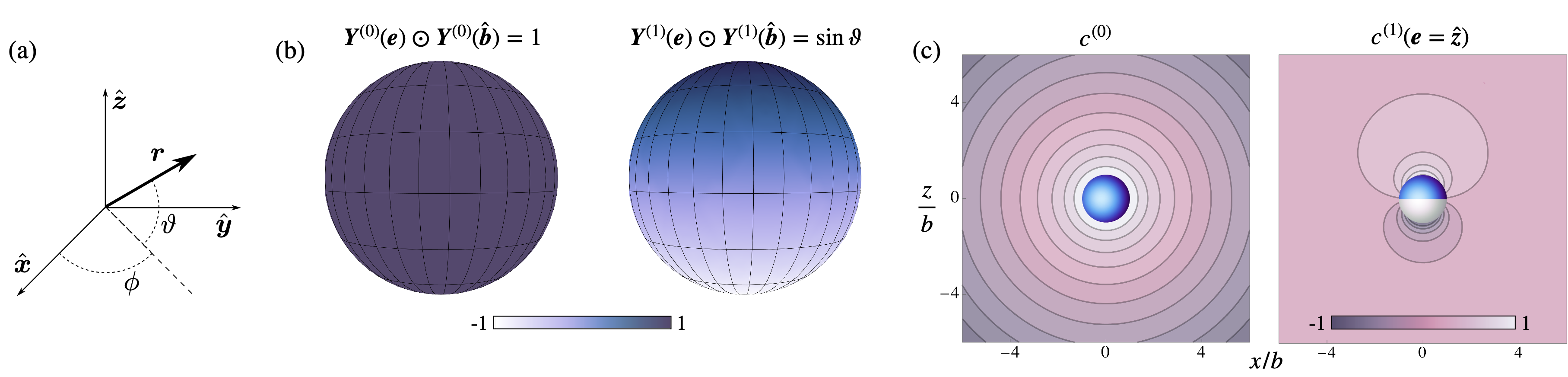
Figure 1: Flux distribution and resulting concentration field. Panel (a) shows our choice of spherical coordinate system with the angle $\vartheta$ to the $x$-$y$ plane. In panel (b) we show the first two modes of the surface densities in the expansion of the surface concentration and the active flux in Eq. (3) and the phoretic mobility in Eq. (26) in terms of TSH. The unit vector $\boldsymbol{e}$ represents the orientation of the respective mode, as is further discussed in Section IV.3, while $\hat{\boldsymbol{b}}$ is the unit radius vector of the sphere. Here, we choose $\boldsymbol{e}=\hat{\boldsymbol{z}}$. Panel (c) shows the concentration fields generated by a particle with the surface flux distributions shown in panel (b) far away from any boundaries. The chemical field lines are plotted as pseudo-colour maps and contours show regions of constant concentration. The particle is schematically represented by a blue sphere (uniform flux, $j^{\mathcal{A}}(\boldsymbol{b})\propto J_{0}>0$, generates $c^{(0)}$) or a blue-white sphere (linear flux, $j^{\mathcal{A}}(\boldsymbol{b})\propto\boldsymbol{J}^{(1)}\cdot\hat{\boldsymbol{b}}$ with $\boldsymbol{J}^{(1)}=J_{1}\boldsymbol{e}$ and $J_{1}>0$, generates $c^{(1)}(\boldsymbol{e})$). Linearity of Laplace equation allows us to superimpose these concentration fields as required. In Section IV we superimpose the two leading modes for the surface flux to emulate a Janus particle with an inert ($j^{\mathcal{A}}=0$) south pole ($\vartheta=-\pi/2$) and an active north pole ($\vartheta=\pi/2$).

To project Eq. (IIe) for the concentration at the surface of the particle onto a linear system, we expand the boundary fields,

$$c(\boldsymbol{b})=\sum_{q=0}^{\infty}w_{q}\boldsymbol{C}^{(q)}\odot\boldsymbol{Y}^{(q)}(\hat{\boldsymbol{b}}),\qquad j^{\mathcal{A}}(\boldsymbol{b})=\sum_{q=0}^{\infty}\tilde{w}_{q}\boldsymbol{J}^{(q)}\odot\boldsymbol{Y}^{(q)}(\hat{\boldsymbol{b}}).$$ (3)

The product denoted by $\odot$ implies a maximal contraction of Cartesian indices (a $q$-fold contraction between a tensor of rank-$q$ and another one of higher rank), and we have defined

$$w_{q}=\frac{1}{q!\left(2q-1\right)!!},\quad\tilde{w}_{q}=\frac{2q+1}{4\pi b^{2}}.$$ (4)

The background concentration field $c^{\infty}(\boldsymbol{b})$ at the surface of the particle is expanded in an analogous manner to $c(\boldsymbol{b})$, with coefficients denoted by $\boldsymbol{C}^{\infty(q)}$. The expansion coefficients $\boldsymbol{C}^{(q)}$ and $\boldsymbol{J}^{(q)}$ are symmetric and traceless tensors of rank-$q$ and the leading modes of this expansion are shown in Figure 1, alongside the generated concentration fields. Linearity of Laplace equation implies that the general solution in a basis of TSH can be written as

$$\boldsymbol{C}^{(q)}=\boldsymbol{\zeta}^{(q,q^{\prime})}\odot\boldsymbol{C}^{\infty(q^{\prime})}+\boldsymbol{\mathcal{E}}^{(q,q^{\prime})}\odot\boldsymbol{J}^{(q^{\prime})},$$ (5)

corresponding to Eq. (IIe), where the task now is to find the connecting tensors $\boldsymbol{\zeta}^{(q,q^{\prime})}$ and $\boldsymbol{\mathcal{E}}^{(q,q^{\prime})}$. In Appendix A, starting from the BIE for the surface concentration and using a Galerkin-Jacobi iterative method, we outline how to find approximate solutions, in leading powers of distance between the particle and surrounding boundaries, for these tensors in terms of a given Green’s function $H$ of Laplace equation (Singh et al., 2019).

Any Green’s function $H$ of Laplace equation can be written as the sum,

$$H(\boldsymbol{R},\tilde{\boldsymbol{R}})=H^{o}(\boldsymbol{r})+H^{*}(\boldsymbol{R},\tilde{\boldsymbol{R}}),$$ (6)

with $\boldsymbol{r}=\boldsymbol{R}-\tilde{\boldsymbol{R}}$, where $\boldsymbol{R}$ and $\tilde{\boldsymbol{R}}$ are the field and the source point, respectively. Here, $H^{o}(\boldsymbol{r})=1/4\pi Dr$ is the fundamental solution of Laplace equation in an unbounded domain. On the other hand, $H^{*}$ is an extra contribution needed to satisfy additional boundary conditions in the system. For the unbounded case, where $H=H^{o}(\boldsymbol{r})$, the single-layer and double-layer operators in Eqs. (IIb) and (IIc) have singular integral kernels. However, due to translational invariance they can be evaluated using Fourier techniques, see Appendix A.1. We find that both integral operators diagonalise simultaneously in a basis of TSH, yielding

$$\boldsymbol{\zeta}^{(q,q^{\prime})}=\zeta_{q}\,\boldsymbol{I}^{(q,q^{\prime})},\qquad\boldsymbol{\mathcal{E}}^{(q,q^{\prime})}=\mathcal{E}_{q}\,\boldsymbol{I}^{(q,q^{\prime})},$$ (7)

where

$$\zeta_{q}=\frac{2q+1}{q+1},\qquad\mathcal{E}_{q}=\frac{b}{D}\frac{\tilde{w}_{q}}{w_{q}}\frac{1}{q+1},$$ (8)

and $\boldsymbol{I}^{(q,q^{\prime})}$ is a tensor with elements $\delta_{qq^{\prime}}$, where the latter denotes a Kronecker delta. The expression for the elastance $\mathcal{E}_{q}$ is confirmed by previous results obtained by first solving the Laplace equation in the fluid volume and subsequently matching the boundary condition (Ic) for the surface flux (Jackson, 1962; Golestanian et al., 2007). If the system contains additional boundaries, we find corrections to these diagonal expressions in terms of derivatives of $H^{*}$. To leading order, this yields

$$\boldsymbol{\zeta}^{(q,q^{\prime})}=\zeta_{q}\left(\boldsymbol{I}^{(q,q^{\prime})}+4\pi bDw_{q^{\prime}}\tfrac{q^{\prime}}{q^{\prime}+1}b^{q+q^{\prime}}\boldsymbol{\nabla}^{(q)}\tilde{\boldsymbol{\nabla}}^{(q^{\prime})}H^{*}(\boldsymbol{R},\tilde{\boldsymbol{R}})\right),$$ (9)

where $\nabla_{\alpha_{1}\dots\alpha_{q}}^{(q)}=\nabla_{\alpha_{1}}\dots\nabla_{\alpha_{q}}$, and where we have introduced the short-hand notation $\boldsymbol{\nabla}_{\boldsymbol{R}}=\boldsymbol{\nabla}$ for derivatives with respect to the field point and $\boldsymbol{\nabla}_{\tilde{\boldsymbol{R}}}=\tilde{\boldsymbol{\nabla}}$ for the source point. The point of evaluation, $\boldsymbol{R}=\tilde{\boldsymbol{R}}$ for the one-body problem, is left implicit for brevity. Similarly, we find for the elastance,

$$\boldsymbol{\mathcal{E}}^{(q,q^{\prime})}=\mathcal{E}_{q}\left(\boldsymbol{I}^{(q,q^{\prime})}+4\pi bD_{1}w_{q}\tfrac{2q^{\prime}+1}{q^{\prime}+1}b^{q+q^{\prime}}\boldsymbol{\nabla}^{(q)}\tilde{\boldsymbol{\nabla}}^{(q^{\prime})}H^{*}(\boldsymbol{R},\tilde{\boldsymbol{R}})\right).$$ (10)

III.2 Hydrodynamic problem and Brownian motion

Using the linearity of Stokes flow we solve for the hydrodynamic traction $\boldsymbol{f}^{H}$ in a basis of TSH. Upon eliminating the hydrodynamic problem, Newton’s equations (1) will reveal the Brownian motion of an active particle. First, to find the linear system corresponding to Eq. (IIk), we expand the slip and the hydrodynamic traction in a basis of TSH,

$$\boldsymbol{v}^{\mathcal{A}}(\boldsymbol{b})=\sum_{l=1}^{\infty}w_{l-1}\boldsymbol{V}^{(l)}\odot\boldsymbol{Y}^{(l-1)}(\hat{\boldsymbol{b}}),\qquad\boldsymbol{f}^{H}(\boldsymbol{b})=\sum_{l=1}^{\infty}\tilde{w}_{l-1}\boldsymbol{F}^{(l)}\odot\boldsymbol{Y}^{(l-1)}(\hat{\boldsymbol{b}}).$$ (11)

The coefficients $\boldsymbol{V}^{(l)}$ and $\boldsymbol{F}^{(l)}$ are rank-$l$ tensors, symmetric and traceless in their last $l-1$ indices. They can be decomposed into irreducible representations, denoted by $\boldsymbol{V}^{(l\sigma)}$ (or $\boldsymbol{F}^{(l\sigma)}$ for the traction moments), where $\boldsymbol{V}^{(ls)}$ (symmetric and traceless), $\boldsymbol{V}^{(la)}$ (anti-symmetric) and $\boldsymbol{V}^{(lt)}$ (trace) are irreducible tensors of rank $l$, $l-1$ and $l-2$, respectively (Singh et al., 2015). For slip restricted by mass conservation only, obeying $\int\boldsymbol{v}^{\mathcal{A}}\cdot\hat{\boldsymbol{b}}{\rm d}S=0$, these irreducible components of $\boldsymbol{V}^{(l)}$ (and $\boldsymbol{F}^{(l)}$) are independent of each other. In terms of the common definitions for the velocity and angular velocity of an active particle in an unbounded domain (Anderson and Prieve, 1991; Stone and Samuel, 1996; Ghose and Adhikari, 2014),

$$\boldsymbol{V}^{\mathcal{A}}=-\frac{1}{4\pi b^{2}}\int\boldsymbol{v}^{\mathcal{A}}(\boldsymbol{b}){\rm d}S,\qquad\boldsymbol{\Omega}^{\mathcal{A}}=-\frac{3}{8\pi b^{3}}\int\hat{\boldsymbol{b}}\times\boldsymbol{v}^{\mathcal{A}}(\boldsymbol{b}){\rm d}S,$$ (12)

we have $\boldsymbol{V}^{(1s)}=-\boldsymbol{V}^{\mathcal{A}}$ and $\boldsymbol{V}^{(2a)}/2b=-\boldsymbol{\Omega}^{\mathcal{A}}.$ Similarly, we have for the hydrodynamic force and torque defined in Eq. (2), $\boldsymbol{F}^{(1s)}=\boldsymbol{F}^{H}$ and $\boldsymbol{F}^{(2a)}=\frac{1}{b}\boldsymbol{T}^{H}$.

Linearity of Stokes equation then allows us to write down the deterministic part of Eq. (IIk) in a basis of TSH,

$$\boldsymbol{F}^{(l\sigma)} =-\boldsymbol{\gamma}^{(l\sigma,1s)}\cdot\boldsymbol{V}-\boldsymbol{\gamma}^{(l\sigma,2a)}\cdot\boldsymbol{\Omega}-\hat{\boldsymbol{\gamma}}^{(l\sigma,l^{\prime}\sigma^{\prime})}\odot\boldsymbol{V}^{(l^{\prime}\sigma^{\prime})},$$ (13)

where $\boldsymbol{\gamma}^{(l\sigma,l^{\prime}\sigma^{\prime})}$ and $\hat{\boldsymbol{\gamma}}^{(l\sigma,l^{\prime}\sigma^{\prime})}$ are generalised friction tensors for rigid body motion and slip, respectively. For the modes corresponding to rigid body motion it is known that $\boldsymbol{\gamma}^{(l\sigma,1s)}=\hat{\boldsymbol{\gamma}}^{(l\sigma,1s)}$ and $\boldsymbol{\gamma}^{(l\sigma,2a)}=\hat{\boldsymbol{\gamma}}^{(l\sigma,2a)}$ (Singh and Adhikari, 2018; Turk et al., 2022). Therefore, we can write for the hydrodynamic force and torque,

$$\begin{pmatrix}\boldsymbol{F}^{H}\\ \boldsymbol{T}^{H}\end{pmatrix}=-\boldsymbol{\Gamma}\cdot\begin{pmatrix}\boldsymbol{V}-\boldsymbol{V}^{\mathcal{A}}\\ \boldsymbol{\Omega}-\boldsymbol{\Omega}^{\mathcal{A}}\end{pmatrix}+\sum_{l\sigma=2s}\hat{\boldsymbol{\Gamma}}^{(l\sigma)}\odot\boldsymbol{V}^{(l\sigma)},\quad\text{with}\quad\boldsymbol{\Gamma}=\begin{pmatrix}\boldsymbol{\gamma}^{TT}&\boldsymbol{\gamma}^{TR}\\ \boldsymbol{\gamma}^{RT}&\boldsymbol{\gamma}^{RR}\end{pmatrix},\quad\hat{\boldsymbol{\Gamma}}^{(l\sigma)}=\begin{pmatrix}\hat{\boldsymbol{\gamma}}^{(T,l\sigma)}\\ \hat{\boldsymbol{\gamma}}^{(R,l\sigma)}\end{pmatrix},$$ (14)

where the superscripts $T$ and $R$ imply $l\sigma=1s,2a$, respectively. The matrix $\boldsymbol{\Gamma}$ contains the friction on the particle due to rigid body motion, and $\hat{\boldsymbol{\Gamma}}^{(l\sigma)}$ contains the friction due to higher modes of slip. This concludes the solution of the hydrodynamic problem without fluctuations.

Inserting this into Newton’s equations (1) yields the Langevin equation

$$\begin{pmatrix}m\dot{\boldsymbol{V}}\\ I\dot{\boldsymbol{\Omega}}\end{pmatrix}=\begin{pmatrix}\boldsymbol{F}^{P}\\ \boldsymbol{T}^{P}\end{pmatrix}-\boldsymbol{\Gamma}\cdot\begin{pmatrix}\boldsymbol{V}-\boldsymbol{V}^{\mathcal{A}}\\ \boldsymbol{\Omega}-\boldsymbol{\Omega}^{\mathcal{A}}\end{pmatrix}+\sum_{l\sigma=2s}\hat{\boldsymbol{\Gamma}}^{(l\sigma)}\odot\boldsymbol{V}^{(l\sigma)}+\sqrt{2k_{B}T\,\boldsymbol{\Gamma}}\cdot\begin{pmatrix}\boldsymbol{\xi}^{T}\\ \boldsymbol{\xi}^{R}\end{pmatrix},$$ (15)

where we have used that in a thermally fluctuating fluid at equilibrium the Brownian forces and torques obey the fluctuation-dissipation relations (Einstein, 1905; Zwanzig, 1964; Chow, 1973; Singh and Adhikari, 2017)

$$\left\langle\begin{pmatrix}\hat{\boldsymbol{F}}(t)\\ \hat{\boldsymbol{T}}(t)\end{pmatrix}\right\rangle=\boldsymbol{0},\qquad\left\langle\begin{pmatrix}\hat{\boldsymbol{F}}(t)\\ \hat{\boldsymbol{T}}(t)\end{pmatrix}\begin{pmatrix}\hat{\boldsymbol{F}}(t^{\prime})\\ \hat{\boldsymbol{T}}(t^{\prime})\end{pmatrix}^{\text{tr}}\right\rangle=2k_{B}T\,\boldsymbol{\Gamma}\,\delta(t-t^{\prime}),$$ (16)

where angled brackets denote ensemble averages, $k_{B}$ is the Boltzmann constant, and $T$ is the temperature, while the transpose is defined as $(A_{\alpha\beta})^{\text{tr}}=A_{\beta\alpha}$. The $\boldsymbol{\xi}^{\alpha}$ represent independent Gaussian white noises. In the inertial equation (15) the noise is not multiplicative since $\boldsymbol{\Gamma}$ is configuration dependent, but not velocity dependent. With the particle centre of mass $\boldsymbol{R}$ and its unit orientation vector $\boldsymbol{e}$ (its orientation is governed by the rotational dynamics $\dot{\boldsymbol{\Theta}}=\boldsymbol{\Omega}$, where $\boldsymbol{\Theta}$ is an arbitrary set of angles), we can find its Brownian trajectory by integrating

$$\dot{\boldsymbol{R}}=\boldsymbol{V},\qquad\dot{\boldsymbol{e}}=\boldsymbol{\Omega}\times\boldsymbol{e},$$ (17)

over time. In colloidal systems the inertia of both the particles and the fluid are typically negligible. This corresponds to the Smoluchowski limit of Eq. (15). Adiabatic elimination of the momentum variables in phase space then directly leads to the following update equations in Itô form (Ermak and McCammon, 1978; Gardiner, 1984; Wajnryb et al., 2004; Volpe and Wehr, 2016),

$$\boldsymbol{R}(t+\Delta t) =\boldsymbol{R}(t)+\Big{\{}\boldsymbol{V}^{\mathcal{A}}+\boldsymbol{\mu}^{TT}\cdot\boldsymbol{F}^{P}+\boldsymbol{\mu}^{TR}\cdot\boldsymbol{T}^{P}+\sum_{l\sigma=2s}\boldsymbol{\pi}^{(T,l\sigma)}\odot\boldsymbol{V}^{(l\sigma)}+k_{B}T\,\tilde{\boldsymbol{\nabla}}\cdot\boldsymbol{\mu}^{TT}\Big{\}}\Delta t+\Delta\hat{\boldsymbol{R}},$$ (18a)

$$\boldsymbol{e}(t+\Delta t) =\boldsymbol{e}(t)+\Big{\{}\boldsymbol{\Omega}^{\mathcal{A}}+\boldsymbol{\mu}^{RT}\cdot\boldsymbol{F}^{P}+\boldsymbol{\mu}^{RR}\cdot\boldsymbol{T}^{P}+\sum_{l\sigma=2s}\boldsymbol{\pi}^{(R,l\sigma)}\odot\boldsymbol{V}^{(l\sigma)}+k_{B}T\,\tilde{\boldsymbol{\nabla}}\cdot\boldsymbol{\mu}^{RT}\Big{\}}\Delta t\times\boldsymbol{e}(t)+\Delta\hat{\boldsymbol{e}},$$ (18b)

with $\Delta\hat{\boldsymbol{e}}=\Delta\hat{\boldsymbol{\Theta}}(t)\times\boldsymbol{e}(t)+\tfrac{1}{2}\Delta\hat{\boldsymbol{\Theta}}(t)\cdot\left[\boldsymbol{e}(t)\Delta\hat{\boldsymbol{\Theta}}(t)-\Delta\hat{\boldsymbol{\Theta}}(t)\boldsymbol{e}(t)\right]$ and the Gaussian white noise

$$\left\langle\begin{pmatrix}\Delta\hat{\boldsymbol{R}}\\ \Delta\hat{\boldsymbol{\Theta}}\end{pmatrix}\right\rangle=\boldsymbol{0},\qquad\left\langle\begin{pmatrix}\Delta\hat{\boldsymbol{R}}\\ \Delta\hat{\boldsymbol{\Theta}}\end{pmatrix}\begin{pmatrix}\Delta\hat{\boldsymbol{R}}\\ \Delta\hat{\boldsymbol{\Theta}}\end{pmatrix}^{\text{tr}}\right\rangle=2k_{B}T\,\mathbb{M}\,\Delta t.$$ (19)

It is clear that the grand mobility matrix $\mathbb{M}$ and the grand propulsion tensor $\boldsymbol{\Pi}^{(l\sigma)}$ satisfy

$$\mathbb{M}=\begin{pmatrix}\boldsymbol{\mu}^{TT}&\boldsymbol{\mu}^{TR}\\ \boldsymbol{\mu}^{RT}&\boldsymbol{\mu}^{RR}\end{pmatrix}=\boldsymbol{\Gamma}^{-1},\qquad\boldsymbol{\Pi}^{(l\sigma)}=\begin{pmatrix}\boldsymbol{\pi}^{(T,l\sigma)}\\ \boldsymbol{\pi}^{(R,l\sigma)}\end{pmatrix}=\mathbb{M}\cdot\hat{\boldsymbol{\Gamma}}^{(l\sigma)}.$$ (20)

Onsager-Casimir symmetry implies symmetry of the mobility matrix, and we can identify the so-called propulsion tensors as $\boldsymbol{\pi}^{(\alpha,l\sigma)}=\boldsymbol{\mu}^{\alpha T}\cdot\hat{\boldsymbol{\gamma}}^{(T,l\sigma)}+\boldsymbol{\mu}^{\alpha R}\cdot\hat{\boldsymbol{\gamma}}^{(R,l\sigma)},$ with $\alpha\in\{T,R\}$ (Singh and Adhikari, 2018). The convective terms in the update equations, proportional to the divergence of the mobility, are commonly assigned the slightly misleading label spurious drift. The occurring derivative $\tilde{\boldsymbol{\nabla}}$ is the standard spatial gradient (with respect to the source point). If the mobilities depend on the particle orientation, additional orientational convective terms must be included. For the spherical particles considered here, however, these terms do not contribute. The quadratic term in $\Delta\boldsymbol{\Theta}$ in $\Delta\hat{\boldsymbol{e}}$ is needed to preserve the condition $|\boldsymbol{e}|=1$ as discussed in (Makino and Doi, 2004; De Corato et al., 2015).

As Stokes equation defines a dissipative system, any acceptable approximation of $\mathbb{M}$ must remain positive definite for all physical configurations, e.g. when a simulated particle does not overlap with nearby boundaries (Cichocki et al., 2000). In Appendix B, starting from the BIE of Stokes flow and using a Galerkin-Jacobi iterative method, we outline how to find such solutions, in principle to arbitrary accuracy in the distance between the particle and surrounding boundaries, for the mobility and propulsion tensors in terms of the Green’s function $\boldsymbol{G}$ of Stokes flow. For this, we write the Green’s function as the sum (Marian Smoluchowski, 1911),

$$\boldsymbol{G}(\boldsymbol{R},\tilde{\boldsymbol{R}})=\boldsymbol{G}^{o}(\boldsymbol{r})+\boldsymbol{G}^{*}(\boldsymbol{R},\tilde{\boldsymbol{R}}),$$ (21)

where $\boldsymbol{r}=\boldsymbol{R}-\tilde{\boldsymbol{R}}$, and $\boldsymbol{G}^{o}(\boldsymbol{r})=\left(\boldsymbol{I}+\hat{\boldsymbol{r}}\hat{\boldsymbol{r}}\right)/8\pi\eta r$ is the Oseen tensor for unbounded Stokes flow (Oseen, 1927; Pozrikidis, 1992). The term $\boldsymbol{G}^{*}$ is the correction necessary to satisfy additional boundary conditions in the system. In the unbounded domain, where $\boldsymbol{G}=\boldsymbol{G}^{o}(\boldsymbol{r})$, the mobility matrix $\mathbb{M}$ diagonalises and the propulsion tensors vanish identically,

$$\boldsymbol{\mu}^{TT}=\mu_{T}\,\boldsymbol{I},\quad\boldsymbol{\mu}^{R}=\mu_{R}\,\boldsymbol{I},\quad\boldsymbol{\mu}^{TR}=\boldsymbol{\mu}^{RT}=\boldsymbol{0},\qquad\boldsymbol{\pi}^{(\alpha,l\sigma)}=\boldsymbol{0}.$$ (22)

Here, $\mu_{T}=\left(6\pi\eta b\right)^{-1}$ and $\mu_{R}=\left(8\pi\eta b^{3}\right)^{-1}$ are the well known mobility coefficients for translation and rotation of a sphere of radius $b$ in an unbounded fluid of viscosity $\eta$ (Stokes, 1850). For a system containing additional boundaries, we obtain corrections to the above expressions in terms of derivatives of $\boldsymbol{G}^{*}$. As shown in the Appendix, to leading order in the Jacobi iteration the mobilities are

$$\boldsymbol{\mu}^{TT}=\mu_{T}\left(\boldsymbol{I}+6\pi\eta b\,\mathcal{F}^{0}\tilde{\mathcal{F}}^{0}\boldsymbol{G}^{*}\right),\qquad\boldsymbol{\mu}^{TR}=\tfrac{1}{2}\mathcal{F}^{0}\,\tilde{\boldsymbol{\nabla}}\times\boldsymbol{G}^{*},\qquad\boldsymbol{\mu}^{RR}=\mu_{R}\,\boldsymbol{I}+\tfrac{1}{2}\boldsymbol{\nabla}\times\boldsymbol{\mu}^{TR}.$$ (23a)

For the differential operator $\mathcal{F}_{i}^{l}=\big{(}1+\frac{b^{2}}{4l+6}\nabla_{i}^{2}\big{)}$, where $i$ is the position vector with respect to which the Laplacian is defined, we have used the shorthand notations $\mathcal{F}_{\boldsymbol{R}}^{l}=\mathcal{F}^{l}$ and $\mathcal{F}_{\tilde{\boldsymbol{R}}}^{l}=\tilde{\mathcal{F}}^{l}$.

Governed by the particle’s activity, we choose to retain the leading symmetric and polar modes of the slip. As demonstrated in the next Section, this requires the following propulsion tensors,

$$\boldsymbol{\pi}^{(T,2s)}=\tfrac{4\pi\eta b^{2}}{3}\mathcal{F}^{0}\tilde{\mathcal{F}}^{1}\left[\tilde{\boldsymbol{\nabla}}\boldsymbol{G}^{*}+(\tilde{\boldsymbol{\nabla}}\boldsymbol{G}^{*})^{\text{tr}}\right],\qquad\boldsymbol{\pi}^{(T,3t)}=-\tfrac{6\pi\eta b^{3}}{25}\mathcal{F}^{0}\tilde{\nabla}^{2}\boldsymbol{G}^{*},\qquad\boldsymbol{\pi}^{(T,4t)}=-\tfrac{38\pi\eta b^{4}}{2205}\mathcal{F}^{0}\tilde{\boldsymbol{\nabla}}\tilde{\nabla}^{2}\boldsymbol{G}^{*},$$ (24a)

given to leading order in the Jacobi iteration. The structure of the problem implies that $\boldsymbol{\pi}^{(R,l\sigma)}=\tfrac{1}{2}\left(\boldsymbol{\nabla}\times\boldsymbol{\pi}^{(T,l\sigma)}\right).$ To the given order these have been first obtained by Singh and Adhikari (2018).

III.3 Chemo-hydrodynamic coupling and resulting propulsion

We now consider the boundary condition (IIl), coupling the hydrodynamic to the chemical problem. We observe that the differential operator $\boldsymbol{\chi}$ defined in Eq. (Ig) implies tangential slip such that $\hat{\boldsymbol{b}}\cdot\boldsymbol{v}^{\mathcal{A}}=0$, i.e., chemical gradients at the surface of the particle can only drive tangential slip flows. Satisfying this condition, we write the tangential modes in the expansion of the slip in Eq. (11) with a subscript $s$ as $\boldsymbol{V}_{s}^{(l\sigma)}$. In order to obey the tangential slip condition, the symmetric and trace modes of the slip expansion coefficients have to satisfy

$$\boldsymbol{V}_{s}^{([l+2]t)}=-l(2l+3)\boldsymbol{V}_{s}^{(ls)}.$$ (25)

This means that whenever a $\boldsymbol{V}_{s}^{(ls)}$ mode is generated, a $\boldsymbol{V}_{s}^{([l+2]t)}$ mode of strength given by Eq. (25) will be generated too. For the anti-symmetric modes $\boldsymbol{V}_{s}^{(la)}$ there is no such condition as they produce tangential slip flow by definition (Singh et al., 2015).

Finally, to express the boundary condition (Ig) in a basis of TSH, we expand the phoretic mobility as

$$\mu_{c}(\boldsymbol{b})=\sum_{q=0}^{\infty}\tilde{w}_{q}\boldsymbol{M}^{(q)}\odot\boldsymbol{Y}^{(q)}(\hat{\boldsymbol{b}}).$$ (26)

The coefficients $\boldsymbol{M}^{(q)}$ are symmetric and traceless tensors of rank-$q$. This yields the linear system corresponding to Eq. (IIl),

$$\boldsymbol{V}_{s}^{(l\sigma)} =\boldsymbol{\chi}^{(l\sigma,q)}\odot\boldsymbol{C}^{(q)}.$$ (27)

The coupling tensor $\boldsymbol{\chi}^{(l\sigma,q)}$ is given in Appendix A.3, and satisfies $\boldsymbol{\chi}^{(l\sigma,0)}=\boldsymbol{0}$, i.e., a uniform surface concentration does not induce slip.

In principle, any form of tangential slip can be generated by the chemo-hydrodynamic coupling in Eq. (27). Here, we only consider the leading polar ($\boldsymbol{V}_{s}^{(3t)}$), chiral ($\boldsymbol{V}_{s}^{(2a)}$) and symmetric ($\boldsymbol{V}_{s}^{(2s)}$) modes. Using Eq. (25), we can identify

$$\boldsymbol{V}^{\mathcal{A}}=-\boldsymbol{V}_{s}^{(1s)}=5\boldsymbol{V}_{s}^{(3t)},\qquad 2b\boldsymbol{\Omega}^{\mathcal{A}}=-\boldsymbol{V}_{s}^{(2a)},\qquad\boldsymbol{V}_{s}^{(2s)}=-14\boldsymbol{V}_{s}^{(4t)}.$$ (28)

In the following we therefore parametrise polar, chiral and symmetric slip by $\boldsymbol{V}^{\mathcal{A}}$, $\boldsymbol{\Omega}^{\mathcal{A}}$ and $\boldsymbol{V}_{s}^{(2s)}$, respectively. With this, the propulsion terms in the update equations (18) are

$$\sum_{l\sigma=2s}\boldsymbol{\Pi}^{(l\sigma)}\odot\boldsymbol{V}^{(l\sigma)}=-5\begin{pmatrix}\boldsymbol{\pi}^{(T,3t)}\\ \boldsymbol{\pi}^{(R,3t)}\end{pmatrix}\cdot\boldsymbol{V}^{\mathcal{A}}+\begin{pmatrix}\boldsymbol{\pi}^{(T,2s)}-14\boldsymbol{\pi}^{(T,4t)}\\ \boldsymbol{\pi}^{(R,2s)}-14\boldsymbol{\pi}^{(R,4t)}\end{pmatrix}\colon\boldsymbol{V}_{s}^{(2s)}$$ (29)

for an autophoretic particle, and Eq. (27) yields

$$\boldsymbol{V}^{\mathcal{A}} =-\tfrac{1}{4\pi b^{3}}\sum_{q=1}^{\infty}\left[\tfrac{q+1}{2q+1}\boldsymbol{M}^{(q-1)}-q(q+1)\boldsymbol{M}^{(q+1)}\right]\odot\boldsymbol{C}^{(q)},$$ (30a)

$$\boldsymbol{\Omega}^{\mathcal{A}} =-\tfrac{3}{8\pi b^{4}}\sum_{q=1}^{\infty}q\boldsymbol{M}^{(q)}\times^{\prime}\boldsymbol{C}^{(q)},$$ (30b)

$$\boldsymbol{V}_{s}^{(2s)} =\tfrac{3}{4\pi b^{3}}\sum_{q=1}^{\infty}\left[\tfrac{1}{2q-1}\boldsymbol{M}^{(q-2)}+\tfrac{3q}{2q+3}\boldsymbol{M}_{{\rm sym}}^{(q)}-q(q+1)(q+2)\boldsymbol{M}^{(q+2)}\right]\odot\boldsymbol{C}^{(q)}.$$ (30c)

For brevity, we have left the solution for $\boldsymbol{C}^{(q)}$ of Eq. (5) implicit. Here, we have defined a cross product for irreducible tensors as $(\boldsymbol{M}^{(q)}\times^{\prime}\boldsymbol{C}^{(q^{\prime})}){}_{\alpha}=\epsilon_{\alpha\beta\gamma}M_{\beta({\scriptscriptstyle Q-1})}^{(q)}C_{\gamma({\scriptscriptstyle Q^{\prime}-1})}^{(q^{\prime})}$ and a symmetric and traceless product contracting $(q-1)$ indices, $(\boldsymbol{M}_{{\rm sym}}^{(q)}\odot\boldsymbol{C}^{(q^{\prime})})_{\alpha\beta}=\Delta_{\alpha\beta,\alpha^{\prime}\beta^{\prime}}^{(2)}M_{\alpha^{\prime}({\scriptscriptstyle Q-1})}^{(q)}C_{\beta^{\prime}({\scriptscriptstyle Q^{\prime}-1})}^{(q^{\prime})}$, where we have used the short-hand notation for indices $Q=\gamma_{1}\gamma_{2}\dots\gamma_{q}$, and $QQ^{\prime}=\gamma_{1}\gamma_{2}\dots\gamma_{q}\kappa_{1}\kappa_{2}\dots\kappa_{q^{\prime}}$ when multiple sets of indices appear (Damour and Iyer, 1991). In Figure 2 we show the fluid flow generated by an autophoretic particle, either due to an external force or torque acting on it or due to the above-mentioned leading modes of symmetric and polar slip.

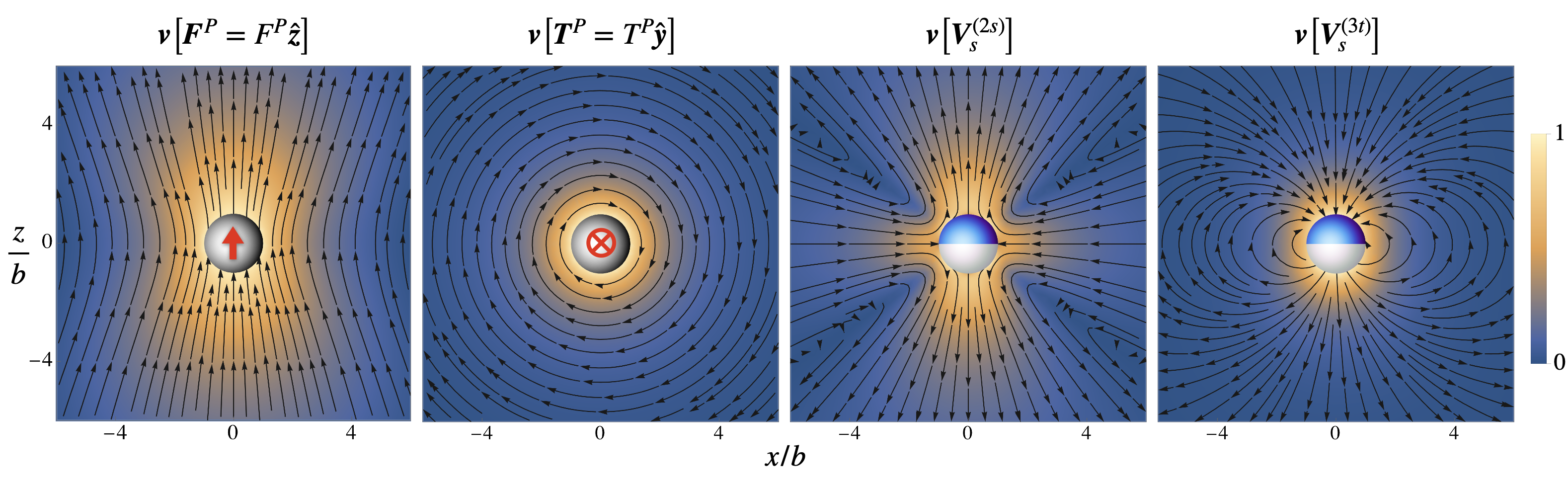
Figure 2: Fluid flow generated by an autophoretic particle far away from boundaries. The particle is schematically represented by a grey (rigid body motion due to external force or torque) or a blue-white (flow due to the leading symmetric, $\boldsymbol{V}_{s}^{(2s)}$, and polar, $\boldsymbol{V}_{s}^{(3t)}=\boldsymbol{V}^{\mathcal{A}}/5$, slip modes) sphere. The direction of external forces and torques is indicated by a red vector. The direction of the fluid flow (lab frame) is indicated by black arrows, while its relative magnitude is implied by the overlaid pseudo-colormap. Linearity of Stokes equation allows us to superimpose these flows as required, see Figure 4 for an application.

IV Autophoresis near an interface

In this section we apply the general results discussed thus far to describe the dynamics of an autophoretic particle near a plane interface. Given its surface flux $j^{\mathcal{A}}$ and phoretic mobility $\mu_{c}$, we sequentially determine the concentration distribution generated at its surface, the thus driven slip flows, and the resulting hydrodynamic Brownian interactions with the interface. For this, we emulate a Janus particle with a non-trivial phoretic mobility distribution on its surface. This can be modelled by the following phoretic mobility and surface flux, truncating the expansions (3) and (26) at linear order,

$$\mu_{c}(\boldsymbol{b})=\tfrac{1}{4\pi b^{2}}\left(M_{0}+3\boldsymbol{M}^{(1)}\cdot\hat{\boldsymbol{b}}\right),\quad\quad j^{\mathcal{A}}(\boldsymbol{b})=\tfrac{1}{4\pi b^{2}}\left(J_{0}+3\boldsymbol{J}^{(1)}\cdot\hat{\boldsymbol{b}}\right).$$ (31)

Choosing $J_{0}/3=J_{1}=J$, where $J_{1}=\left|\boldsymbol{J}^{(1)}\right|$, the particle has one inert pole ($j^{\mathcal{A}}=0$) and one active pole ($j^{\mathcal{A}}>0$ ($j^{\mathcal{A}}<0$) for $J>0$ ($J<0$), corresponding to a source (sink) of chemical reactants), see Figure 1b. As we will see below, a non-trivial phoretic mobility distribution can lead to interesting effects such as autophoretic self-rotation even in the absence of boundaries.

Region	Chemical Green’s function	Hydrodynamic Green’s function
$z>0$	$\quad H(\boldsymbol{R},\tilde{\boldsymbol{R}})=H^{o}(\boldsymbol{r})+\tfrac{1-\lambda^{c}}{1+\lambda^{c}}H^{o}(\boldsymbol{r}^{*})$	$\,\,G_{\alpha\beta}(\boldsymbol{R},\tilde{\boldsymbol{R}})=G_{\alpha\beta}^{o}(\boldsymbol{r})+\mathcal{M}_{\beta\gamma}^{f}G_{\alpha\gamma}^{o}(\boldsymbol{r}^{*})-2h\frac{\lambda^{f}}{1+\lambda^{f}}\nabla_{\gamma}^{*}G_{\alpha z}^{o}(\boldsymbol{r}^{*})\mathcal{M}_{\beta\gamma}$
		$+h^{2}\frac{\lambda^{f}}{1+\lambda^{f}}\nabla^{*2}G_{\alpha\gamma}^{o}(\boldsymbol{r}^{*})\mathcal{M}_{\beta\gamma}$
$z<0$	$\quad H(\boldsymbol{R},\tilde{\boldsymbol{R}})=\tfrac{2\lambda^{c}}{1+\lambda^{c}}H^{o}(\boldsymbol{r})$	$\,\,G_{\alpha\beta}(\boldsymbol{R},\tilde{\boldsymbol{R}})=\frac{\lambda^{f}}{1+\lambda^{f}}\left[2\delta_{\beta\rho}G_{\alpha\rho}^{o}(\boldsymbol{r})-2h\nabla_{\beta}G_{\alpha z}^{o}(\boldsymbol{r})-h^{2}\nabla^{2}G_{\alpha\beta}^{o}(\boldsymbol{r})\right]$

Table 3: Green’s functions for a plane interface. The Green’s functions for the concentration (Laplace equation, left) and velocity (Stokes equation, right) fields near a plane, chemically permeable fluid-fluid interface of solute diffusivity ratio $\lambda^{c}=D_{2}/D_{1}$ and viscosity ratio $\lambda^{f}=\eta_{2}/\eta_{1}$ at $z=0$ are given. The particle is in the positive half-space $z>0$, where the solute diffusivity is $D_{1}$ and the fluid viscosity is $\eta_{1}$. We use $\boldsymbol{r}=\boldsymbol{R}-\tilde{\boldsymbol{R}}$ and $\boldsymbol{r}^{*}=\boldsymbol{R}-\tilde{\boldsymbol{R}}^{*}$, with the field point $\boldsymbol{R}=\left(x,y,z\right)^{\text{tr}}$ , the source point $\tilde{\boldsymbol{R}}=(\tilde{x},\tilde{y},\tilde{z})^{\text{tr}}$ and the relation $\tilde{\boldsymbol{R}}^{*}=\boldsymbol{\mathcal{M}}\cdot\tilde{\boldsymbol{R}}$ between the physical position vector $\tilde{\boldsymbol{R}}$ and the position vector of the image singularities $\tilde{\boldsymbol{R}}^{*}$. The height of the centre of the particle above the interface is $\tilde{z}=h$. With this, we have $\tilde{\boldsymbol{R}}-\tilde{\boldsymbol{R}}^{*}=(0,0,2h)^{\text{tr}}.$ We define $\boldsymbol{\nabla}^{*}=\boldsymbol{\nabla}_{\boldsymbol{r}^{*}}$, $\mathcal{M}_{\beta\gamma}^{f}=\frac{1-\lambda^{f}}{1+\lambda^{f}}\delta_{\beta\rho}\delta_{\rho\gamma}-\delta_{\beta z}\delta_{z\gamma}$, the mirroring operator $\mathcal{M}_{\beta\gamma}=\delta_{\beta\rho}\delta_{\rho\gamma}-\delta_{\beta z}\delta_{z\gamma}$ and the index $\rho=x,y$ in the plane of the interface.

The plane interface of viscosity ratio $\lambda^{f}=\eta_{2}/\eta_{1}$ and solute diffusivity ratio $\lambda^{c}=D_{2}/D_{1}$ is characterised by the Green’s functions in Table 3. Here, $H$ satisfies the boundary condition of continuous normal flux $\hat{\boldsymbol{z}}\cdot\boldsymbol{j}^{(1)}=\hat{\boldsymbol{z}}\cdot\boldsymbol{j}^{(2)}$ across the interface, and $\boldsymbol{G}$ arises from the boundary conditions of continuous tangential flow $v_{\rho}^{(1)}=v_{\rho}^{(2)},$ vanishing normal flow $v_{z}^{(1)}=v_{z}^{(2)}=0,$ and continuous tangential stress $\eta_{1}\sigma_{\rho z}^{(1)}=\eta_{2}\sigma_{\rho z}^{(2)}$ across the interface, where the index $\rho=x,y$ lies in the plane of the interface (Jones et al., 1975; Aderogba and Blake, 1978). The superscripts label whether the quantity of interest is above or below the interface, where $(1)$ refers to the positive half-space $z>0$.

IV.1 Induced surface concentration

The particle’s surface flux $j^{\mathcal{A}}$ generates a concentration field in the surrounding fluid that qualitatively depends on the boundary condition $\lambda^{c}$, the ratio $J_{0}/J_{1}$ and the orientation of the particle. At the surface of the particle, we choose to truncate the generated concentration field at second order,

$$c(\boldsymbol{b})=C_{0}+\boldsymbol{C}^{(1)}\cdot\hat{\boldsymbol{b}}+\tfrac{1}{6}\boldsymbol{C}^{(2)}\colon\left(3\hat{\boldsymbol{b}}\hat{\boldsymbol{b}}-\boldsymbol{I}\right).$$ (32)

The coefficients are determined by Eq. (5). For a Janus particle near a plane interface, the relevant tensors $\boldsymbol{\zeta}^{(q,q^{\prime})}$ and $\boldsymbol{\mathcal{E}}^{(q,q^{\prime})}$ follow. As the coefficient $C_{0}$ does generate a slip, see Eq. (27), we can ignore terms such as $\boldsymbol{\zeta}^{(0,q)}$ and $\boldsymbol{\mathcal{E}}^{(0,q)}$. From Eq. (9), we further obtain the vanishing contributions $\boldsymbol{\zeta}^{(q,0)}=\boldsymbol{0}$ due to a constant background concentration. Cylindrical symmetry of the system can then be used to write the remaining non-zero chemical tensors in terms of scalar coefficients, which are given in Table 4.

Tensors	Scalar coefficients
$\boldsymbol{\zeta}^{(1,1)}$	$\quad\zeta_{\parallel}^{(1,1)}=\zeta_{1}\left[1+\frac{1}{16}\Lambda^{c}\hat{h}^{-3}\right]$,            $\quad\zeta_{\perp}^{(1,1)}=\zeta_{1}\left[1+\frac{1}{8}\Lambda^{c}\hat{h}^{-3}\right]$
$\boldsymbol{\mathcal{E}}^{(1,0)}$	$\quad\mathcal{E}^{(1,0)}=-\tfrac{1}{4}\mathcal{E}_{1}\Lambda^{c}\hat{h}^{-2}$
$\boldsymbol{\mathcal{E}}^{(1,1)}$	$\quad\mathcal{E}_{\parallel}^{(1,1)}=\mathcal{E}_{1}\left[1+\frac{3}{16}\Lambda^{c}\hat{h}^{-3}\right]$,            $\quad\mathcal{E}_{\perp}^{(1,1)}=\mathcal{E}_{1}\left[1+\frac{3}{8}\Lambda^{c}\hat{h}^{-3}\right]$
$\boldsymbol{\mathcal{E}}^{(2,0)}$	$\quad\mathcal{E}^{(2,0)}=-\tfrac{3}{4}\mathcal{E}_{2}\Lambda^{c}\hat{h}^{-3}$
$\boldsymbol{\mathcal{E}}^{(2,1)}$	$\quad\mathcal{E}^{(2,1)}=-\tfrac{3}{64}\mathcal{E}_{2}\Lambda^{c}\hat{h}^{-4}$

Table 4: Chemical coefficients. Scalar coefficients for the linear response to a background concentration field and for the elastance tensors with $\Lambda^{c}=\left(1-\lambda^{c}\right)/\left(1+\lambda^{c}\right)$, where $\lambda^{c}=D_{2}/D_{1}$, and the height above the interface $\hat{h}=h/b$. We have used the exact unbounded coefficients in Eq. (8) such that $\zeta_{1}=3/2$, $\mathcal{E}_{1}=3/8\pi bD_{1},$ and $\mathcal{E}_{2}=5/2\pi bD_{1}$. Cylindrical symmetry of the system implies for the coupling to a linear background concentration field, $\boldsymbol{\zeta}^{(1,1)}=(\boldsymbol{I}-\hat{\boldsymbol{z}}\hat{\boldsymbol{z}})\,\zeta_{\parallel}^{(1,1)}+\hat{\boldsymbol{z}}\hat{\boldsymbol{z}}\,\zeta_{\perp}^{(1,1)}$. The relevant elastance tensors are $\boldsymbol{\mathcal{E}}^{(1,0)}=\hat{\boldsymbol{z}}\,\mathcal{E}^{(1,0)},$ $\boldsymbol{\mathcal{E}}^{(1,1)}=(\boldsymbol{I}-\hat{\boldsymbol{z}}\hat{\boldsymbol{z}})\,\mathcal{E}_{\parallel}^{(1,1)}+\hat{\boldsymbol{z}}\hat{\boldsymbol{z}}\,\mathcal{E}_{\perp}^{(1,1)},$ $\boldsymbol{\mathcal{E}}^{(2,0)}=-\left(3\hat{\boldsymbol{z}}\hat{\boldsymbol{z}}-\boldsymbol{I}\right)\,\mathcal{E}^{(2,0)},$ and $\mathcal{E}_{\alpha\beta\gamma}^{(2,1)}=\mathcal{E}^{(2,1)}\left[\left(\delta_{\gamma\alpha}-\delta_{\gamma z}\delta_{\alpha z}\right)\delta_{\beta z}+\left(\delta_{\gamma\beta}-\delta_{\gamma z}\delta_{\beta z}\right)\delta_{\alpha z}+\left(3\delta_{\beta z}\delta_{\alpha z}-\delta_{\alpha\beta}\right)\delta_{\gamma z}\right].$

IV.2 Mobility and propulsion tensors

The anisotropic surface concentration in Eq. (32) induces a slip flow. A fluid flow is generated in the surrounding fluid that qualitatively depends on the boundary condition $\lambda^{f}$, any present body force $\boldsymbol{F}^{P}$ or torque $\boldsymbol{T}^{P}$, and the phoretic mobility distribution at the surface of the Janus particle. The fluid then reacts back on the particle and causes rigid body motion, governed by the equations of motion in Eq. (18), mediated by mobility and propulsion tensors.

Again, the cylindrical symmetry of the system allows us to write the mobility and propulsion tensors in terms of scalar coefficients, summarised in Table 5.

Tensors	Scalar coefficients
$\boldsymbol{\mu}^{TT}$	$\quad\mu_{\parallel}^{TT}=\mu_{T}\left[1+\frac{3(2-3\lambda^{f})}{16(1+\lambda^{f})}\hat{h}^{-1}+\frac{1+2\lambda^{f}}{16(1+\lambda^{f})}\hat{h}^{-3}-\frac{\lambda^{f}}{16(1+\lambda^{f})}\hat{h}^{-5}\right]$
	$\quad\mu_{\perp}^{TT}=\mu_{T}\left[1-\frac{3(2+3\lambda^{f})}{8(1+\lambda^{f})}\hat{h}^{-1}+\frac{1+4\lambda^{f}}{8(1+\lambda^{f})}\hat{h}^{-3}-\frac{\lambda^{f}}{8(1+\lambda^{f})}\hat{h}^{-5}\right]$
$\boldsymbol{\mu}^{RR}$	$\quad\mu_{\parallel}^{RR}=\mu_{R}\left[1+\frac{1-5\lambda^{f}}{16(1+\lambda^{f})}\hat{h}^{-3}\right]$
	$\quad\mu_{\perp}^{RR}=\mu_{R}\left[1+\frac{1-\lambda^{f}}{8(1+\lambda^{f})}\hat{h}^{-3}\right]$
$\boldsymbol{\mu}^{TR}$	$\quad\mu^{TR}=\frac{1}{6\pi\eta b^{2}}\left[-\frac{3}{16(1+\lambda^{f})}\hat{h}^{-2}+\frac{3\lambda^{f}}{32(1+\lambda^{f})}\hat{h}^{-4}\right]$
$\boldsymbol{\pi}^{(T,2s)}$	$\quad\pi_{1}^{(T,2s)}=\frac{\lambda^{f}}{8(1+\lambda^{f})}\hat{h}^{-2}-\frac{1+3\lambda^{f}}{30(1+\lambda^{f})}\hat{h}^{-4}+\frac{\lambda^{f}}{24(1+\lambda^{f})}\hat{h}^{-6}$
	$\quad\pi_{2}^{(T,2s)}=-\frac{2+3\lambda^{f}}{24(1+\lambda^{f})}\hat{h}^{-2}+\frac{4+15\lambda^{f}}{120(1+\lambda^{f})}\hat{h}^{-4}-\frac{\lambda^{f}}{24(1+\lambda^{f})}\hat{h}^{-6}$
$\boldsymbol{\pi}^{(T,3t)}$	$\quad\pi_{\parallel}^{(T,3t)}=-\frac{3\left(1+2\lambda^{f}\right)}{400(1+\lambda^{f})}\hat{h}^{-3}+\frac{3\lambda^{f}}{200(1+\lambda^{f})}\hat{h}^{-5}$
	$\quad\pi_{\perp}^{(T,3t)}=-\frac{3\left(1+4\lambda^{f}\right)}{200(1+\lambda^{f})}\hat{h}^{-3}+\frac{3\lambda^{f}}{100(1+\lambda^{f})}\hat{h}^{-5}$
$\boldsymbol{\pi}^{(T,4t)}$	$\quad\pi_{1}^{(T,4t)}=\frac{19\left(1+3\lambda^{f}\right)}{23520\left(1+\lambda^{f}\right)}\hat{h}^{-4}-\frac{19\lambda^{f}}{7056\left(1+\lambda^{f}\right)}\hat{h}^{-6}$
	$\quad\pi_{2}^{(T,4t)}=-\frac{19\left(1+5\lambda^{f}\right)}{23520\left(1+\lambda^{f}\right)}\hat{h}^{-4}+\frac{19\lambda^{f}}{7056\left(1+\lambda^{f}\right)}\hat{h}^{-6}$
$\boldsymbol{\pi}^{(R,2s)}$	$\quad\pi^{(R,2s)}=\frac{1}{b}\left[\frac{1}{16}\hat{h}^{-3}-\frac{\lambda^{f}}{20(1+\lambda^{f})}\hat{h}^{-5}\right]$
$\boldsymbol{\pi}^{(R,3t)}$	$\quad\pi^{(R,3t)}=\frac{1}{b}\frac{9\lambda^{f}}{400(1+\lambda^{f})}\hat{h}^{-4}$
$\boldsymbol{\pi}^{(R,4t)}$	$\quad\pi^{(R,4t)}=\frac{1}{b}\frac{19\lambda^{f}}{5880\left(1+\lambda^{f}\right)}\hat{h}^{-5}$

Table 5: Hydrodynamic coefficients. Scalar coefficients for the mobility matrices and the relevant propulsion tensors with $\lambda^{f}=\eta_{2}/\eta_{1}$ and the height above the interface $\hat{h}=h/b$. Cylindrical symmetry of the system allows us to write for the translational mobilities, $\boldsymbol{\mu}^{TT}=(\boldsymbol{I}-\hat{\boldsymbol{z}}\hat{\boldsymbol{z}})\mu_{\parallel}^{TT}+\hat{\boldsymbol{z}}\hat{\boldsymbol{z}}\mu_{\perp}^{TT}$ and $\boldsymbol{\mu}^{TR}=\left(\boldsymbol{\mu}^{RT}\right)^{\text{tr}}=\mu^{TR}\boldsymbol{\epsilon}\cdot\hat{\boldsymbol{z}}$. The mobility $\boldsymbol{\mu}^{RR}$ has the same structure as $\boldsymbol{\mu}^{TT}$ with the corresponding coefficients $\mu_{\parallel}^{RR}$ and $\mu_{\perp}^{RR}$. The propulsion tensor for the leading symmetric slip mode is $\pi_{\alpha\beta\gamma}^{(T,2s)}=\pi_{1}^{(T,2s)}\left[\left(\delta_{\gamma\alpha}-\delta_{\gamma z}\delta_{\alpha z}\right)\delta_{\beta z}+\left(\delta_{\beta\alpha}-\delta_{\beta z}\delta_{\alpha z}\right)\delta_{\gamma z}\right]+\pi_{2}^{(T,2s)}\left(\delta_{\gamma\beta}-3\delta_{\gamma z}\delta_{\beta z}\right)\delta_{\alpha z}$. The propulsion tensor $\boldsymbol{\pi}^{(T,4t)}$ is of the same structure as $\boldsymbol{\pi}^{(T,2s)}$ with the corresponding coefficients $\pi_{1}^{(T,4t)}$ and $\pi_{2}^{(T,4t)}$. Since $\boldsymbol{\pi}^{(T,3t)}$ has the same structure as $\boldsymbol{\mu}^{TT}$, we adopt an analogous notation with $\pi_{\parallel}^{(T,3t)}$ and $\pi_{\perp}^{(T,3t)}$. For the propulsion tensors contributing to the particle’s rotational dynamics we obtain $\pi_{\alpha\beta\gamma}^{(R,2s)}=\pi^{(R,2s)}\left(\delta_{\beta z}\epsilon_{z\gamma\alpha}+\delta_{\gamma z}\epsilon_{z\beta\alpha}\right)$ and $\boldsymbol{\pi}^{(R,3t)}=\pi^{(R,3t)}\boldsymbol{\epsilon}\cdot\hat{\boldsymbol{z}}$. The propulsion tensor $\boldsymbol{\pi}^{(R,4t)}$ is of the same structure as $\boldsymbol{\pi}^{(R,2s)}$ with the corresponding coefficient $\pi^{(R,4t)}$.

These mobility coefficients have been obtained in the literature to a varying degree of accuracy. Most notably, for the most symmetric problem of a particle sedimenting towards a plane surface the problem has been solved exactly (Brenner, 1961). For motion parallel to a plane wall ($\lambda^{f}\rightarrow\infty$), providing asymptotic lubrication-theory-like solutions, the above results for $\boldsymbol{\mu}^{TT}$, $\boldsymbol{\mu}^{RR}$ and $\boldsymbol{\mu}^{TR}$ are obtained to the given order in (Goldman et al., 1967a) with an additional term of order $\hat{h}^{-4}$, discussed in Appendix B. Using so-called antenna theorems (Felderhof, 1976), numerical results to high accuracy (up to order $\hat{h}^{-20}$) are found for the mobilities of motion near a free surface ($\lambda^{f}=0$) and a plane wall (Perkins and Jones, 1990, 1992), matching our results to the order given. A method of reflections has been used to analytically find the mobility coefficients for a general viscosity ratio $\lambda^{f}$ up to leading order in $\hat{h}^{-1}$ (Lee et al., 1979), with numerically evaluated exact results derived in bi-polar coordinates (Lee and Leal, 1980). It is readily shown that our analytical results for the mobilities match these numerically evaluated results very well for the full range of viscosity ratios $\lambda^{f}$ down to particle-boundary gaps of order unity.

In the absence of an exact solution for motion parallel to a boundary, careful examination of the case when the particle-interface gap distance is much smaller than the particle radius is necessary. In 1967, Goldman, Cox and Brenner (Goldman et al., 1967b) used a lubrication approximation to derive an asymptotic solution for this case. However, matching the asymptotic solutions for the near- ($h\ll b$) and far-field ($h\gg b$) limits can be challenging in dynamic simulations (Brady and Bossis, 1988; Ichiki, 2002). Furthermore, for motion parallel to the plane it has recently been confirmed experimentally that the order to which the mobilities are given in Table 5 provides a good approximation even when the particle-interface gap distance is only a fraction of the particle radius (Choudhury et al., 2017). So while an approach using lubrication theory is appropriate for general motion very close to a plane (Villa et al., 2020, 2023), the given approximation arising from a series expansion can still be expected to be of interest to a wide range of experimental settings in which colloidal particles are studied near a plane boundary. In particular, in Appendix C we show that for the plane boundary the diffusion terms $\propto\sqrt{2k_{B}T\,\mathbb{M}}$ in Eqs. (18) take a particularly simple analytic form and that with the coefficients given in Table 5 this diffusion matrix is inherently positive definite for all physical configurations. While analytical and numerical results are available in the literature for the mobilities, the propulsion tensors are a unique feature of active particles and have not been obtained in this form in the literature.

IV.3 Bottom-heavy Brownian Janus particle

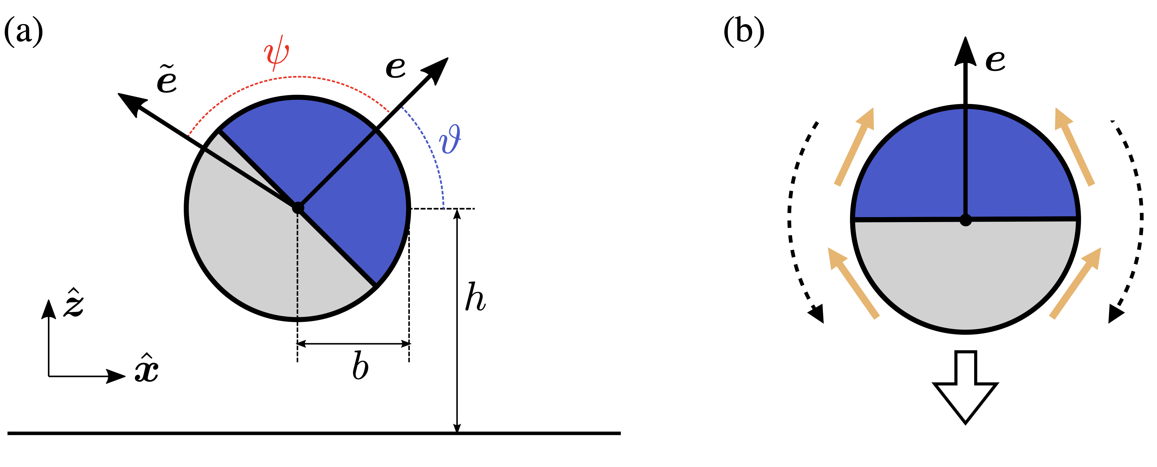
Figure 3: Janus particle. Schematic representation of a Janus particle (blue and white implying actively coated and inert sides, respectively) with the vectorial coefficient of the surface flux $\boldsymbol{J}^{(1)}$ is oriented along $\boldsymbol{e}$, see Eq. (33). (a) A particle of radius $b$ at a height $h$ from a plane boundary. The vectorial coefficient of the phoretic mobility $\boldsymbol{M}^{(1)}$ is oriented along $\tilde{\boldsymbol{e}}$, at a fixed relative angle $\psi$ to $\boldsymbol{e}$. (b) Janus particle in an unbounded domain (Golestanian et al., 2007), assuming $\psi=0$ and $J>0$ (source-swimmer). The active flux along $\boldsymbol{e}$ produces chemical gradients, resulting in a flux of $c$ along the dashed arrows. Assuming $\mu_{c}>0$ this generates a slip flow along the yellow arrows (see the panel denoted by $\boldsymbol{V}_{s}^{(3t)}$ in Figure 2 for the resulting fluid flow) and thus, due to fluid stresses reacting back on the particle, a net particle velocity in the direction of the thick open arrow, i.e., inert-face forward swimming. For $J<0$ (sink-swimmer) the particle swims active-face forward in the direction of $\boldsymbol{e}$.

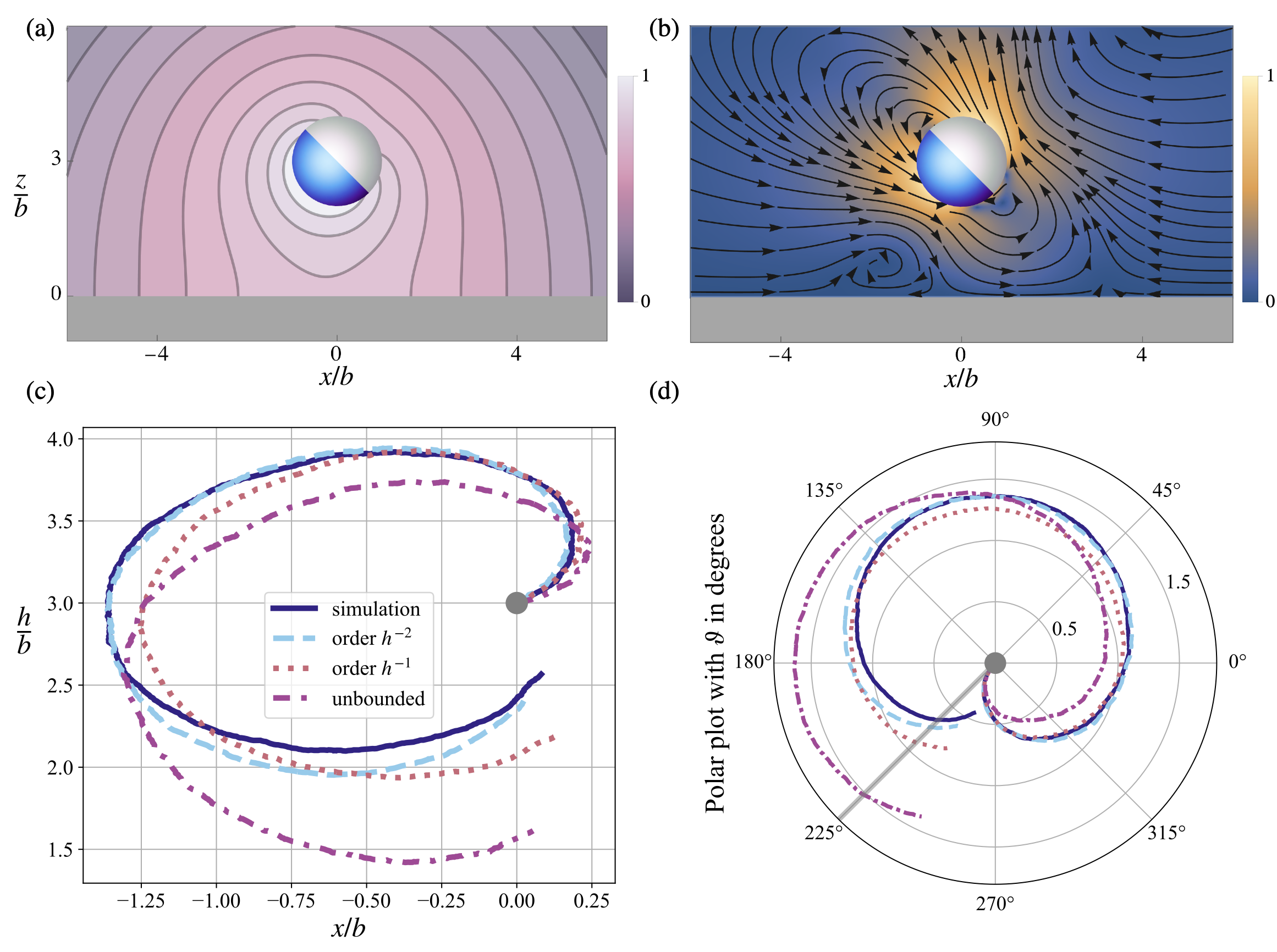
Figure 4: Wall-effects on autophoresis. We compare typical trajectories of a bottom-heavy autophoretic particle (see Section IV.3 for the chosen particle specifications) suspended in a fluctuating fluid at a height $\hat{h}=h/b$ above a plane no-slip and no-flux wall ($\lambda^{f}\rightarrow\infty$, $\lambda^{c}=0$) at various approximations in $\hat{h}^{-1}$ of the equations of motion (18). In panels (a) and (b) the particle is schematically represented by a Janus particle, see Figure 3. The starting point of the particle in panels (c) and (d) is indicated by a grey disk. (a) The contours of the concentration field generated by the particle. It is worthwhile to note that here the contour lines are perpendicular to the wall (a ‘no-flux’ boundary) and the corresponding vector field ($\boldsymbol{\nabla}c$) is purely tangential. (b) The deterministic part of the fluid flow due to the particle’s slip and bottom-heaviness. The stresses created in the fluid react back on the particle and cause self-propulsion. (c) We compare the trajectories of the particle obtained to various orders in $\hat{h}^{-1}$, thus gradually including more interactions with the wall. Here, ‘simulation’ refers to the full dynamical system at the accuracy obtained in this paper. It is clear that the approximations converge towards this simulation with increasing orders of $\hat{h}^{-1}$ included. (d) Orientational evolution of the particle in the various approximations in a polar plot, parametrised by the angle $\vartheta$ and the distance to the starting point. The thick grey line indicates the initial orientation $\vartheta_{0}$ of the particle. To order $\hat{h}^{-1}$ the orientational dynamics are unaffected by the wall.

We now parametrise the Janus particle obeying (31) by setting

$$\boldsymbol{J}^{(1)}=J_{1}\boldsymbol{e},\quad\quad\boldsymbol{M}^{(1)}=M_{1}\tilde{\boldsymbol{e}},$$ (33)

where $\boldsymbol{e}$ and $\tilde{\boldsymbol{e}}$ are unit orientation vectors, related by a particle-specific constant angle $\psi$ such that $\tilde{\boldsymbol{e}}\times\boldsymbol{e}=\sin\psi$, see Figure 3a. For simplicity, we assume the absence of any background concentration field. Due to cylindrical symmetry of the system, and assuming there is no external torque rotating the particle out of plane, i.e., $\boldsymbol{T}^{P}\cdot\hat{\boldsymbol{z}}=0$, we can restrict our attention to the $x$-$z$ plane for which we define the planar polar angle $\vartheta\in\left\{-\pi,\pi\right\}$ (see Figure 1a for a coordinate system) such that

$$\boldsymbol{e}=\cos\vartheta\,\hat{\boldsymbol{x}}+\sin\vartheta\,\hat{\boldsymbol{z}},\quad\quad\tilde{\boldsymbol{e}}=\cos\left(\vartheta+\psi\right)\,\hat{\boldsymbol{x}}+\sin\left(\vartheta+\psi\right)\,\hat{\boldsymbol{z}}.$$ (34)

We fix $\boldsymbol{e}$ as the orientation of the particle. It is important to note, however, that $\boldsymbol{e}$ is not in general the direction of propulsion, as is shown in Figure 3b for a source swimmer with $J>0$ in an unbounded domain.

Autophoretic particles in typical experiments are neither force nor torque free due to mismatches between particle and solvent densities and between gravitational and geometric centres (Ebbens and Howse, 2010; Drescher et al., 2010; Palacci et al., 2010, 2013; Buttinoni et al., 2013). Since the resulting forces and torques become dominant, at long distances, over active contributions, it is crucial to include their effects in our analysis. In simulating Eq. (17) we therefore assume a bottom-heavy Janus particle (the chemically active coating, blue in figures, is assumed to be slightly heavier than the inert side, white in figures). Therefore, we have to take into account gravity in negative $z$-direction and a gravitational torque given by

$$\boldsymbol{F}^{P}=-mg\hat{\boldsymbol{z}},\qquad\boldsymbol{T}^{P}=\kappa(\hat{\boldsymbol{z}}\times\boldsymbol{e})=\kappa\cos\vartheta\,\hat{\boldsymbol{y}},$$ (35)

with $m$ the buoyancy-corrected mass of the particle, $g$ the gravitational constant, and $\kappa$ a constant parametrising bottom-heaviness.

Inserting this into the update equations (18) with $\boldsymbol{R}=(x,y,h)^{\text{tr}}$, where $h(t)$ is the height of the particle above the boundary, we can now simulate the time-evolution of a bottom-heavy Brownian Janus particle. In Figure 4 we show a typical trajectory for a source-particle ($J>0$) with non-trivial phoretic mobility ($M_{1},\psi\neq 0$) near an inert no-slip wall ($\lambda^{f}\rightarrow\infty$, $\lambda^{c}=0$). We probe the effect of the nearby boundary on the dynamics of the autophoretic particle by truncating the dynamical system in Eq. (17) at various orders in $h^{-1}$ and comparing the results, see Appendix C for the truncated expressions.

At order $h^{0}$ (unbounded) it is clear that even for a force- and torque-free particle ($g=\kappa=0$) in an unbounded fluid, phoretic self-propulsion occurs for the Janus particle given by Eq. (31). In particular, for $\psi\neq 0$ the particle is capable of phoretic self-rotation. At order $h^{-1}$ hydrodynamic interactions with the boundary due to the gravitational force manifest themselves. At this order, chemical interactions with the boundary do not yet appear and compared to the unbounded case, only the dynamics in the direction perpendicular to the wall are affected. At order $h^{-2}$ the gravitational torque, and active effects become apparent. The latter comprise hydrodynamic interactions from symmetric propulsion via $\boldsymbol{\pi}^{(T,2s)}$ and a purely chemical interaction with the interface due to the active monopole term $J_{0}$. At this order in the approximation, fore-aft symmetry breaking of the particle is no longer necessary for self-propulsion near a boundary, see Appendix C. An isotropic particle with uniform phoretic mobility $\mu_{c}$ and surface flux $j^{\mathcal{A}}$ will get repelled (attracted) to the interface depending on whether it is a source or sink of chemical reactants and depending on the diffusivity ratio $\lambda^{c}$ of the interface. This self-propulsion of isotropic particles near a boundary has been observed in light-activated phoretic swimmers (Palacci et al., 2013). Furthermore, at this order in the approximation the thermal advective term in Eq. (18) proportional to $\boldsymbol{\nabla}\cdot\mathbb{M}$ starts to affect the dynamics. It is worth noting that at order $h^{-3}$ our analytical results match those obtained by (Ibrahim and Liverpool, 2015), using a method of reflections, for a Janus particle of trivial phoretic mobility near an inert no-slip wall.

The system parameters in Figure 4 are chosen as follows. The starting position of the particle is at a height $\hat{h}_{0}=h(t=0)/b=3$ and an angle $\vartheta_{0}=-3\pi/4$ to the wall. For the surface flux of the particle we choose the dimensionless control parameter $\alpha=J_{1}/J_{0}=1/3$, modelling a source particle. Its phoretic mobility distribution is specified by the dimensionless parameter $\beta=M_{1}/M_{0}=0.6$, implying a significant non-isotropy ($\beta=0$ specifies a trivial phoretic mobility). The angle between the axes of surface flux and phoretic mobility is chosen such that $\psi=\pi/2$. The typical active force on a particle moving at a speed $v_{s}=|\boldsymbol{V}^{\mathcal{A}}|$ is $F_{A}\sim 6\pi\eta b\,v_{s}$, while typical Brownian forces are of the order $\mathcal{O}(\hat{F}_{0})$, where $\hat{F}_{0}=k_{B}T/b$. The dimensionless ratio $\mathcal{B_{T}}=\hat{F}_{0}/F_{A}$ of typical Brownian to active forces has been referred to as Brown number (Singh and Adhikari, 2018), and is set to $\mathcal{B_{T}}\approx 3.4\times 10^{-4}$ in our simulation. In a set of experiments on Janus colloids (Jiang et al., 2010; Palacci et al., 2013), the size $b\sim 1\mu m$, and the speed $v_{s}\sim 10\mu ms^{-1}$ leads to $F_{A}\sim 10^{-13}N$, which implies a Brown number of $\mathcal{B_{T}}\sim 10^{-2}$. To make the hydrodynamic and chemical particle-wall interactions feature more prominently in Figure 4, we have chosen to simulate a lower level of noise than observed in these particular experiments. Similarly, the typical active torque on a particle rotating at a speed $\omega_{s}=|\boldsymbol{\Omega}^{\mathcal{A}}|$ is $T_{A}\sim 8\pi\eta b^{3}\,\omega_{s}$. Brownian torques are of the order $\mathcal{O}(\hat{T}_{0})$, where $\hat{T}_{0}=k_{B}T$. In our simulation, the rotational Brown number, $\mathcal{B_{R}}=\hat{T}_{0}/T_{A}$, the ratio of typical Brownian to active torques, is chosen such that $\mathcal{B_{R}}\approx 1.9\times 10^{-4}$. Additionally, the ratios of gravitational to active forces and torques are chosen such that $mg/F_{A}\approx 3.4\times 10^{-1}$ and $\kappa/T_{A}\approx 1.9\times 10^{-2}$, respectively. Finally, inertial effects decay on the time-scale of momentum relaxation, typically $\tau_{{}_{T}}=m/6\pi\eta b$ and $\tau_{R}=I/8\pi\eta b^{3}=m/20\pi\eta b$ for translational and rotational effects, respectively. The time step $\Delta t$ in our simulation is chosen such that $\tau_{T}/\Delta t\approx 2\times 10^{-4}$ and $\tau_{R}/\Delta t\approx 6\times 10^{-5}$, ensuring that the Smoluchowski limit of the dynamics provides an appropriate description.

V Discussion

In this paper, we have presented a simultaneous solution of the boundary-domain integral equations describing the chemical and the fluid flow around an autophoretic particle in a fluctuating environment. This has been achieved in a basis of tensor spherical harmonics. Compared to the common squirmer model approach to active particles (Lighthill, 1952; Blake, 1971; Pak and Lauga, 2014; Pedley et al., 2016), our boundary-domain integral method offers the distinct advantage of obtaining the traction on the particle directly in a complete orthonormal basis. This provides a naturally kinetic approach via Newton’s equations in which thermal fluctuations manifest themselves as fluctuating stresses. The Brownian motion of an autophoretic particle is obtained in terms of coupled roto-translational stochastic update equations containing mobility and propulsion tensors. The latter are found to arise from chemical activity of the particle and the chemo-hydrodynamic coupling at the particle’s surface, inducing a coupling of slip modes. We have obtained exact and leading-order solutions for both the chemical and the fluctuating hydrodynamic problems far away from and in the vicinity of boundaries, respectively. In the case of autophoresis near a plane interface of fixed viscosity ratio and solute permeability, we have provided readily available analytical expressions for the chemical coupling tensors, and the mobility and propulsion tensors, ensuring a positive definite diffusion matrix. Finally, we have demonstrated our method by studying the dynamical system for a bottom-heavy Brownian Janus particle.

Here, we have given the leading order results for the chemical and hydrodynamic coupling tensors. In principle, these can be obtained to arbitrary accuracy, and the general iterative solutions are given in the Appendix. This non-trivial computation will be the topic of future work. While our results in Section III.2 are guaranteed to provide dissipative motion for physical configurations, in Brownian simulations, unphysical situations with a non-zero particle-boundary overlap may occur on occasion (the probability of which can be lowered by imposing a short-range repulsive potential between the particle and the boundary). In this case, one can either impose an ad-hoc regularisation to the mobility (Wajnryb et al., 2013; Singh and Adhikari, 2017; Balboa Usabiaga et al., 2017) or use a bounce-back condition, effectively implementing a reflective boundary condition in simulation (Volpe et al., 2014). In Section IV, when simulating a Brownian autophoretic particle near a wall, we implemented the latter.

It is helpful to compare our results with previous work on chemical and hydrodynamic interactions of an active particle in a fluctuating fluid. The chemical fields generated by autophoretic particles have been studied extensively (Golestanian et al., 2007; Ebbens and Howse, 2010; Illien et al., 2017; Lisicki et al., 2018; Kanso and Michelin, 2019; Daddi-Moussa-Ider et al., 2018). At the same time, explicit analytical results for the one-body elastance are only present for unbounded domains or near an inert no-slip wall that is impermeable to solutes (Golestanian et al., 2007; Ibrahim and Liverpool, 2015; Uspal et al., 2015; Singh et al., 2019). To the best of our knowledge, this is the first work to obtain the elastance for an active particle near an interface separating two fluids of arbitrary diffusivity ratios in terms of a Green’s function of the Laplace equation that satisfies appropriate boundary conditions. In addition, this Green’s function, which is given in Table 3, does not appear anywhere in the literature, although its derivation is straightforward given the correct boundary conditions. This paper is also the first to simultaneously study the chemo-hydrodynamics of an active particle near a plane surface separating two fluctuating fluids with an arbitrary ratio of viscosities and diffusivities using the boundary-domain integral equations of Stokes and Laplace equations. In particular, for the hydrodynamic problem, we have obtained explicit expression for the propulsion tensors needed for simulation of active particles near an interface of arbitrary viscosity ratio. Thus, our work adds to the existing literature on computing the mobility (Brenner, 1961; Goldman et al., 1967a; Felderhof, 1976; Perkins and Jones, 1990, 1992; Lee et al., 1979; Lee and Leal, 1980; Swan and Brady, 2007; Daddi-Moussa-Ider et al., 2018; Michailidou et al., 2009) and diffusion (Ermak and McCammon, 1978; Wajnryb et al., 2004; Rogers et al., 2012; Delong et al., 2015; Lisicki et al., 2016) of a micro-particle near a boundary. Explicit expressions for propulsion tensors and mobility matrices are given in 5, while Table 4 contains explicit expressions for the connectors of autophoresis near an interface. These will be helpful in Langevin simulations of autophoretic particles in various experimentally realisable settings and for studying fluctuating trajectories of an active particle including both chemical and hydrodynamic interactions.

Aside from its intrinsic theoretical significance, the single-body solution (exact away from boundaries and approximate in complex environments) holds potential value in numerically solving the boundary-domain integral equation for multiple particles. This is due to the ability to initiate numerical iterations with the single-body solution. For problems falling under this category, discretised versions of the boundary-domain integral equations result in diagonally dominant linear systems. Notably, the one-body solution serves as the solution in cases where hydrodynamic interactions are disregarded. This implies that starting iterations from the one-body solution can lead to rapid convergence towards diagonally dominant numerical solutions (Singh and Adhikari, 2018). In scenarios involving multiple interacting particles, utilising a basis of tensor spherical harmonics for expanding surface fields offers distinct advantages over other bases like spherical or vector spherical harmonics, including reduced computational cost due to covariance under rotations (Greengard and Rokhlin, 1987; Damour and Iyer, 1991; Applequist, 2002; Turk, 2023). The condition for tangential slip flow in terms of TSH in Eq. (25) now connects in a straightforward way the formalism for general slip (restricted by mass conservation only) used in previous works (Ghose and Adhikari, 2014; Singh et al., 2015; Singh and Adhikari, 2018; Singh et al., 2019; Turk et al., 2022) to the present and other problems in which tangential slip is considered, e.g. active drops.

In future work we will analytically and numerically build upon the theoretical results contained in this paper, including the aim for a detailed analysis of the zero-temperature limit of the dynamical system in Eq. (18) governing autophoresis near an interface, including the search for bound states (Bolitho et al., 2020), potentially relevant to the study of biofilm formation in bacteria (Wilking et al., 2011; Persat et al., 2015).

Appendix A Chemical problem

A.1 Exact solution for integral equations

As discussed in a previous work (Singh et al., 2019) using Galerkin’s method , the BIE (IIa) can be expressed as the linear system

$$\tfrac{1}{2}\boldsymbol{C}^{(q)}=\boldsymbol{C}^{\infty(q)}+\boldsymbol{\mathcal{H}}^{(q,q^{\prime})}\odot\boldsymbol{J}^{(q^{\prime})}+\boldsymbol{\mathcal{L}}^{(q,q^{\prime})}\odot\boldsymbol{C}^{(q^{\prime})},$$ (36)

with the matrix elements

$$\boldsymbol{\mathcal{H}}^{(q,q^{\prime})}(\boldsymbol{R},\tilde{\boldsymbol{R}})=\tilde{w}_{q}\tilde{w}_{q^{\prime}}\int\boldsymbol{Y}^{(q)}(\hat{\boldsymbol{b}})H(\boldsymbol{R}+\boldsymbol{b},\tilde{\boldsymbol{R}}+\boldsymbol{b}^{\prime})\boldsymbol{Y}^{(q^{\prime})}(\hat{\boldsymbol{b}}^{\prime}){\rm d}S{\rm d}S^{\prime},$$ (37a)

$$\boldsymbol{\mathcal{L}}^{(q,q^{\prime})}(\boldsymbol{R},\tilde{\boldsymbol{R}})=\tilde{w}_{q}w_{q^{\prime}}\int\boldsymbol{Y}^{(q)}(\hat{\boldsymbol{b}})\hat{\boldsymbol{b}}^{\prime}\cdot\boldsymbol{L}(\boldsymbol{R}+\boldsymbol{b},\tilde{\boldsymbol{R}}+\boldsymbol{b}^{\prime})\boldsymbol{Y}^{(q^{\prime})}(\hat{\boldsymbol{b}}^{\prime}){\rm d}S{\rm d}S^{\prime}.$$ (37b)

Here, we evaluate these integrals for an unbounded domain, when $H=H^{o}(\boldsymbol{r})$ (see Eq. (6)) and $\boldsymbol{L}=\boldsymbol{L}^{o}(\boldsymbol{r})$, given by $\boldsymbol{L}^{o}(\boldsymbol{r})=\hat{\boldsymbol{r}}/4\pi r^{2}$. The matrix elements for the unbounded domain have singular but integrable kernels. Due to their translational invariance they can be solved using Fourier techniques. The derivation follows analogous steps to the one of the exact solution for the Stokes traction for an isolated active particle in (Turk et al., 2022). Writing $\boldsymbol{\mathcal{H}}^{o(q,q^{\prime})}$ and $\boldsymbol{\mathcal{L}}^{o(q,q^{\prime})}$ for the corresponding matrix elements, we find

$$\mathcal{H}_{QQ^{\prime}}^{o(q,q^{\prime})}=\sum_{n,n^{\prime}=0}^{\infty}\tau_{nn^{\prime}qq^{\prime}}\int{\rm d}SY_{Q}^{(q)}(\hat{\boldsymbol{b}})Y_{N}^{(n)}(\hat{\boldsymbol{b}})\int{\rm d}S^{\prime}Y_{Q^{\prime}}^{(q^{\prime})}(\hat{\boldsymbol{b}}^{\prime})Y_{N^{\prime}}^{(n^{\prime})}(\hat{\boldsymbol{b}}^{\prime})\\ \times\int{\rm d}kj_{n}(kb)j_{n^{\prime}}(kb)\int{\rm d}\Omega_{k}Y_{N}^{(n)}(\hat{\boldsymbol{k}})k^{2}\hat{H}^{o}(\boldsymbol{k})Y_{N^{\prime}}^{(n^{\prime})}(\hat{\boldsymbol{k}}),$$ (38)

for the single-layer and similarly for the double-layer,

$$\mathcal{L}_{QQ^{\prime}}^{o(q,q^{\prime})}=\sum_{l,l^{\prime}=0}^{\infty}\tau_{nn^{\prime}qq^{\prime}}\int{\rm d}SY_{Q}^{(q)}(\hat{\boldsymbol{b}})Y_{N}^{(n)}(\hat{\boldsymbol{b}})\int{\rm d}S^{\prime}Y_{Q^{\prime}}^{(q^{\prime})}(\hat{\boldsymbol{b}}^{\prime})Y_{N^{\prime}}^{(n^{\prime})}(\hat{\boldsymbol{b}}^{\prime})\boldsymbol{Y}^{(1)}(\hat{\boldsymbol{b}}^{\prime})\\ \times\int{\rm d}kkj_{n}(kb)j_{n^{\prime}}(kb)\int{\rm d}\Omega_{k}Y_{N}^{(n)}(\hat{\boldsymbol{k}})k\hat{\boldsymbol{L}}^{o}(\boldsymbol{k})Y_{N^{\prime}}^{(n^{\prime})}(\hat{\boldsymbol{k}}).$$ (39)

Here, we have defined $\tau_{nn^{\prime}qq^{\prime}}=\tfrac{2b^{4}}{\pi}i^{n+3n^{\prime}}\tilde{w}_{q}\tilde{w}_{q^{\prime}}w_{n}\tilde{w}_{n}w_{n^{\prime}}\tilde{w}_{n^{\prime}}$ and used the Fourier transforms of the Green’s functions for the unbounded domain,

$$\hat{H}^{o}(\boldsymbol{k})=\frac{1}{D}\frac{1}{k^{2}},\qquad\hat{\boldsymbol{L}}^{o}(\boldsymbol{k})=i\frac{\hat{\boldsymbol{k}}}{k}.$$ (40)

The functions $j_{n}(kb$) are spherical Bessel functions, $b=|\boldsymbol{b}|$, and $i=\sqrt{-1}$ is the imaginary unit. Further, $\int{\rm d}S$ implies an integral over the surface of a sphere with radius $b$, $\int{\rm d}\Omega$ the integral over the surface of a unit sphere, and $\int{\rm d}k$ a scalar definite integral from $0$ to $\infty$. Evaluating these expressions, we find that the single- and double-layer matrix elements diagonalise simultaneously in a basis of TSH such that

$$\boldsymbol{\mathcal{H}}^{o(q,q^{\prime})}\odot\boldsymbol{J}^{(q^{\prime})}=\frac{1}{4\pi bDw_{q}}\boldsymbol{J}^{(q)},\qquad\boldsymbol{\mathcal{L}}^{o(q,q^{\prime})}\odot\boldsymbol{C}^{(q^{\prime})}=-\frac{1}{2(2q+1)}\boldsymbol{C}^{(q)}.$$ (41)

The linear system in Eq. (36) can then be solved trivially. We find the exact result, valid for an arbitrary mode index $q$,

$$\boldsymbol{C}^{(q)}=\zeta_{q}\boldsymbol{C}^{\infty(q)}+\mathcal{E}_{q}\boldsymbol{J}^{(q)}.$$ (42)

with $\zeta_{q}$ and $\mathcal{E}_{q}$ given in Eq. (42). In deriving this result, we corrected an error in the double-layer calculation given in (Singh et al., 2019).

For the matrix elements due to additional boundary conditions with the propagator $H^{*}$ and the corresponding double-layer $L^{*}$ it is known that Eqs. (37) evaluate to (Singh et al., 2019)

$$\boldsymbol{\mathcal{H}}^{*(q,q^{\prime})}=b^{q+q^{\prime}}\boldsymbol{\nabla}^{(q)}\tilde{\boldsymbol{\nabla}}^{(q^{\prime})}H^{*}(\boldsymbol{R},\tilde{\boldsymbol{R}}),\qquad\boldsymbol{\mathcal{L}}^{*(q,q^{\prime})}=\frac{4\pi bD}{(q^{\prime}-1)!(2q^{\prime}+1)!!}\boldsymbol{\mathcal{H}}^{*(q,q^{\prime})},$$ (43)

where we have left the point of evaluation, $\boldsymbol{R}=\tilde{\boldsymbol{R}}$ for the one-body problem, implicit for brevity, and where $\boldsymbol{\mathcal{L}}^{*(q,q^{\prime})}$ is defined for $q^{\prime}\geq 1$.

A.2 Iterative solution in complex environments

The formal solution of the boundary-domain integral equation for the concentration field in Eq. (IId) in a basis of TSH gives the following for the linear response to a background concentration field,

$$\boldsymbol{\zeta}^{(q,q^{\prime})}=\left[\boldsymbol{A}^{-1}\right]^{(q,q^{\prime})},\qquad{\rm where}\qquad\boldsymbol{A}^{(q,q^{\prime})}=\left(\tfrac{1}{2}\boldsymbol{I}-\boldsymbol{\mathcal{L}}\right)^{(q,q^{\prime})}.$$ (44)

This can be computed using Jacobi’s iterative method of matrix inversion. At the $n$-th iteration, we find

$$\left(\boldsymbol{\zeta}^{(q,q^{\prime})}\right)^{[n]}=\left(\boldsymbol{A}^{(q,q)}\right)^{-1}\Big{[}\boldsymbol{I}^{(q,q^{\prime})}-\sum^{{}^{\prime}}\boldsymbol{A}^{(q,q^{\prime\prime})}\left(\boldsymbol{\zeta}^{(q^{\prime\prime},q^{\prime})}\right)^{[n-1]}\Big{]},\quad{\rm with}\quad\left(\boldsymbol{\zeta}^{(q,q^{\prime})}\right)^{[0]}=\zeta_{q}\boldsymbol{I}^{(q,q^{\prime})}.$$ (45)

The primed sum implies that diagonal terms with $q=q^{\prime\prime}$ are not included. Naturally, we choose the solution in the unbounded domain as the zeroth order solution. Similarly, it is known that at the $n$-th iteration the elastance in a basis of TSH is given by (Singh et al., 2019)

$$\left(\boldsymbol{\mathcal{E}}^{(q,q^{\prime})}\right)^{[n]}=\left(\boldsymbol{A}^{(q,q)}\right)^{-1}\Big{[}\boldsymbol{\mathcal{H}}^{(q,q^{\prime})}-\sum^{{}^{\prime}}\boldsymbol{A}^{(q,q^{\prime\prime})}\left(\boldsymbol{\mathcal{E}}^{(q^{\prime\prime},q^{\prime})}\right)^{[n-1]}\Big{]},\quad{\rm with}\quad\left(\boldsymbol{\mathcal{E}}^{(q,q^{\prime})}\right)^{[0]}=\mathcal{E}_{q}\boldsymbol{I}^{(q,q^{\prime})}.$$ (46)

To first order in the iteration this yields the expressions given in Eqs. (9) and (10), with an error $\mathcal{O}_{a}$ given in Table 7.

A.3 Chemo-hydrodynamic coupling

The chemo-hydrodynamic coupling tensors in a basis of TSH in Eqs. (Ih) and (27) are in general given by the surface integral

$$\boldsymbol{\chi}^{(l,q)}=\tfrac{1}{b}\tilde{w}_{l-1}\sum_{q^{\prime}=0}^{\infty}w_{q}\tilde{w}_{q^{\prime}}\boldsymbol{M}^{(q^{\prime})}\int\left\{(q+1)\boldsymbol{Y}^{(1)}\boldsymbol{Y}^{(l-1)}\boldsymbol{Y}^{(q^{\prime})}\boldsymbol{Y}^{(q)}-\boldsymbol{Y}^{(l-1)}\boldsymbol{Y}^{(q^{\prime})}\boldsymbol{Y}^{(q+1)}\right\}{\rm d}S.$$ (47)

For the leading polar, chiral and symmetric modes of slip we have evaluated them in Eq. (30). This corrects a previously erroneous result (Singh et al., 2019).

Appendix B Hydrodynamic problem and rigid body motion

In the following we include the rigid body motion of the particle, $\boldsymbol{v}^{\mathcal{D}}(\boldsymbol{b})=\boldsymbol{V}+\boldsymbol{\Omega}\times\boldsymbol{b}$, in the expansion in Eq. (11) such that $\boldsymbol{V}^{(1s)}=\boldsymbol{V}-\boldsymbol{V}^{\mathcal{A}}$ and $\boldsymbol{V}^{(2a)}/2b=\boldsymbol{\Omega}-\boldsymbol{\Omega}^{\mathcal{A}}$ for simplicity of notation. As discussed in previous work using a Galerkin method (Singh et al., 2015), the BIE (IIf) for Stokes flow without thermal fluctuations can be expressed as the linear system

$$\tfrac{1}{2}\boldsymbol{V}^{(l\sigma)}=-\boldsymbol{\mathcal{G}}^{(l\sigma,l^{\prime}\sigma^{\prime})}\odot\boldsymbol{F}^{(l^{\prime}\sigma^{\prime})}+\boldsymbol{\mathcal{K}}^{(l\sigma,l^{\prime}\sigma^{\prime})}\odot\boldsymbol{V}^{(l^{\prime}\sigma^{\prime})}.$$ (48)

The matrix elements corresponding to the single- and double layer integrals are

$$\boldsymbol{\mathcal{G}}^{(l,l^{\prime})}(\boldsymbol{R},\tilde{\boldsymbol{R}}) =\tilde{w}_{l-1}\tilde{w}_{l^{\prime}-1}\int\boldsymbol{Y}^{(l-1)}(\hat{\boldsymbol{b}})\boldsymbol{G}(\boldsymbol{R}+\boldsymbol{b},\tilde{\boldsymbol{R}}+\boldsymbol{b}^{\prime})\boldsymbol{Y}^{(l^{\prime}-1)}(\hat{\boldsymbol{b}}^{\prime}){\rm d}S{\rm d}S^{\prime},$$ (49a)

$$\boldsymbol{\mathcal{K}}^{(l,l^{\prime})}(\tilde{\boldsymbol{R}},\boldsymbol{R}) =\tilde{w}_{l-1}w_{l^{\prime}-1}\int\boldsymbol{Y}^{(l-1)}(\hat{\boldsymbol{b}})\boldsymbol{K}(\tilde{\boldsymbol{R}}+\boldsymbol{b}^{\prime},\boldsymbol{R}+\boldsymbol{b})\cdot\hat{\boldsymbol{b}}^{\prime}\boldsymbol{Y}^{(l^{\prime}-1)}(\hat{\boldsymbol{b}}^{\prime}){\rm d}S{\rm d}S^{\prime}.$$ (49b)

In defining the double-layer matrix element it is worthwhile noting the following. Both double-layer integrals (IIc) and (IIh) in Table 2 are defined as improper integrals when $\boldsymbol{r}\in S$, usually referred to as the principal value. This definition differs from the Cauchy principal value of a singular one-dimensional integral. While the latter requires excluding small intervals around the singularity and taking the limit as their size tends to zero simultaneously, the double-layer integrals both are weakly singular (given $S$ is a Lyapunov surface), and so their principal value exists in the usual sense of an improper integral and is a continuous function in $\boldsymbol{r}\in S$ (Pozrikidis, 1992; Kim and Karrila, 1991).

Writing the matrix elements as a sum of unbounded and correction terms, it is known that they evaluate to (Singh et al., 2015; Turk et al., 2022)

$$\boldsymbol{\mathcal{G}}^{(l,l^{\prime})} =\boldsymbol{\mathcal{G}}^{o(l,l^{\prime})}+\boldsymbol{\mathcal{G}}^{*(l,l^{\prime})}=\boldsymbol{\mathcal{G}}^{o(l,l^{\prime})}+b^{l+l^{\prime}-2}\mathcal{F}^{l-1}\tilde{\mathcal{F}}^{l^{\prime}-1}\boldsymbol{\nabla}^{(l-1)}\tilde{\boldsymbol{\nabla}}^{(l^{\prime}-1)}\boldsymbol{G}^{*}(\boldsymbol{R},\tilde{\boldsymbol{R}}),$$ (50a)

$$\boldsymbol{\mathcal{K}}^{(l,l^{\prime})} =\boldsymbol{\mathcal{K}}^{o(l,l^{\prime})}+\boldsymbol{\mathcal{K}}^{*(l,l^{\prime})}$$

$$=\boldsymbol{\mathcal{K}}^{o(l,l^{\prime})}+\frac{4\pi b^{l+l^{\prime}-1}}{(l^{\prime}-2)!(2l^{\prime}-1)!!}\mathcal{F}^{l-1}\tilde{\mathcal{F}}^{l^{\prime}-1}\boldsymbol{\nabla}^{(l-1)}\tilde{\boldsymbol{\nabla}}^{(l^{\prime}-2)}\boldsymbol{K}^{*}(\tilde{\boldsymbol{R}},\boldsymbol{R}).$$ (50b)

These expressions are exact for a spherical particle.

Defining the column vectors for the force and torque acting on the particle $\boldsymbol{F}^{A}=\left(\boldsymbol{F}^{(1s)},\boldsymbol{F}^{(2a)}\right)^{\text{tr}},$the higher moments of traction $\boldsymbol{F}^{B}=\left(\boldsymbol{F}^{(2s)},\boldsymbol{F}^{(3t)},\dots\right)^{\text{tr}}$, the modes corresponding to rigid body motion $\boldsymbol{V}^{A}=\left(\boldsymbol{V}^{(1s)},\boldsymbol{V}^{(2a)}\right)^{\text{tr}},$ and the higher modes of the slip $\boldsymbol{V}^{B}=\left(\boldsymbol{V}^{(2s)},\boldsymbol{V}^{(3t)},\dots\right)^{\text{tr}}$, we can write the linear system as (Singh et al., 2015)

$$\frac{1}{2}\begin{pmatrix}\boldsymbol{V}^{A}\\ \boldsymbol{V}^{B}\end{pmatrix}=-\begin{pmatrix}\boldsymbol{\mathcal{G}}^{AA}&\boldsymbol{\mathcal{G}}^{AB}\\ \boldsymbol{\mathcal{G}}^{BA}&\boldsymbol{\mathcal{G}}^{BB}\end{pmatrix}\begin{pmatrix}\boldsymbol{F}^{A}\\ \boldsymbol{F}^{B}\end{pmatrix}+\begin{pmatrix}\boldsymbol{\mathcal{K}}^{AA}&\boldsymbol{\mathcal{K}}^{AB}\\ \boldsymbol{\mathcal{K}}^{BA}&\boldsymbol{\mathcal{K}}^{BB}\end{pmatrix}\begin{pmatrix}\boldsymbol{V}^{A}\\ \boldsymbol{V}^{B}\end{pmatrix}.$$ (51)

To be able to solve this infinite linear system, we need to truncate the mode expansions (11) at some appropriate order, and fix the gauge-freedom in the traction. Taking care of the latter, we impose $\int\boldsymbol{f}^{H}\cdot\hat{\boldsymbol{b}}{\rm d}S=\,-\int p{\rm d}S=0$, which is equivalent to imposing $F^{(2t)}=0$. The rationale behind this can be explained as follows. The pressure is a harmonic function, i.e., $\nabla^{2}p=0$, and can thus be expanded in a basis constructed from derivatives of $1/r$. The leading mode of such an expansion decays as $1/r$ and its expansion coefficient is obtained from the integral $\int p\,{\rm d}S$. Further, incompressibility, and the absence of sinks and sources of fluid render the pressure a non-dynamical quantity, meaning that the fundamental solution for the fluid flow $\boldsymbol{v}$ is independent of the pressure and decays as $1/r$. However, Stokes equation (Id) must still be satisfied, and a pressure term decaying as $1/r$ would violate it. We thus impose $\int p\,\mathrm{d}S=0$, rendering the single-layer operator invertible. Eliminating the unknown $\boldsymbol{F}^{B}$, we can directly solve for the rigid body motion of the particle,

$$\boldsymbol{V}^{A}=-\mathbb{M}\cdot\boldsymbol{F}^{A}+\boldsymbol{\Pi}\odot\boldsymbol{V}^{B},$$ (52)

where we have defined the grand mobility matrix $\mathbb{M}$ and the grand propulsion tensor $\boldsymbol{\Pi}$,

$$\mathbb{M}=\left[\boldsymbol{\mathcal{G}}^{AA}-\boldsymbol{\mathcal{G}}^{AB}\left(\boldsymbol{\mathcal{G}}^{BB}\right)^{-1}\boldsymbol{\mathcal{G}}^{BA}\right],\qquad\boldsymbol{\Pi}=\left[\boldsymbol{\mathcal{K}}^{AB}+\boldsymbol{\mathcal{G}}^{AB}\left(\boldsymbol{\mathcal{G}}^{BB}\right)^{-1}\left(\tfrac{1}{2}\boldsymbol{I}-\boldsymbol{\mathcal{K}}^{BB}\right)\right].$$ (53)

In finding this solution, we have used that rigid body motion lies in the eigenspace of the double layer matrix element with a uniform eigenvalue of $-1/2$, and that no exterior flows are produced for the rigid body component of the motion such that

$$\boldsymbol{\mathcal{K}}^{AA}\boldsymbol{V}^{A}=-\tfrac{1}{2}\boldsymbol{V}^{A},\quad\quad\boldsymbol{\mathcal{K}}^{BA}\mathbf{V}^{A}=\mathbf{0}.$$ (54)

Equation 53 guarantees a positive-definite mobility matrix given that every principle sub-matrix of a positive definite matrix (here, $\boldsymbol{\mathcal{G}}^{(l\sigma,l^{\prime}\sigma^{\prime})}$) is positive definite itself. Comparing Eqs. (18) and (53) we can directly identify the mobility and propulsion tensors in terms of the matrix elements in Eq. (49). For the mobilities we find

$$\boldsymbol{\mu}^{\alpha\beta}=\frac{1}{c^{\alpha}q^{\beta}}\Big{[}\boldsymbol{\mathcal{G}}^{(l\sigma,l^{\prime}\sigma^{\prime})}-\sum_{l^{\prime\prime}\sigma^{\prime\prime}=2s}\boldsymbol{\mathcal{G}}^{(l\sigma,l^{\prime\prime}\sigma^{\prime\prime})}\boldsymbol{\Upsilon}{}^{(l^{\prime\prime}\sigma^{\prime\prime},l^{\prime}\sigma^{\prime})}\Big{]},$$ (55)

with $\alpha=T,R$ implying $l\sigma=1s,2a$, and $\beta=T,R$ implying $l^{\prime}\sigma^{\prime}=1s,2a$, respectively. The scalar pre-factors $c^{\alpha}$ and $q^{\beta}$ can be found in Table 6.

$\alpha,\beta$	$T$	$R$
$c^{\alpha}$	$1$	$2b$
$q^{\beta}$	$1$	$b$

Table 6: Coefficients $c^{\alpha}$ and $q^{\beta}$ in the mobility and propulsion tensors.

Similarly, we find for the propulsion tensors

$$\boldsymbol{\pi}^{(\alpha,l^{\prime}\sigma^{\prime})}=\frac{1}{c^{\alpha}}\Big{[}\boldsymbol{\mathcal{K}}^{(l\sigma,l^{\prime}\sigma^{\prime})}+\sum_{l^{\prime\prime}\sigma^{\prime\prime}=2s}\boldsymbol{\mathcal{G}}^{(l\sigma,l^{\prime\prime}\sigma^{\prime\prime})}\boldsymbol{\Phi}^{(l^{\prime\prime}\sigma^{\prime\prime},l^{\prime}\sigma^{\prime})}\Big{]}.$$ (56)

The propulsion tensors are defined for $l^{\prime}\sigma^{\prime}\geq 2s$ as follows directly from the equations of motion (18). In Eqs. (55) and (56) we have defined

$$\boldsymbol{\Upsilon}^{(l\sigma,l^{\prime}\sigma^{\prime})} =\sum_{l^{\prime\prime}\sigma^{\prime\prime}=2s}\left(\boldsymbol{\mathcal{G}}^{(l\sigma,l^{\prime\prime}\sigma^{\prime\prime})}\right)^{-1}\boldsymbol{\mathcal{G}}^{(l^{\prime\prime}\sigma^{\prime\prime},l^{\prime}\sigma^{\prime})},$$ (57a)

$$\boldsymbol{\Phi}^{(l\sigma,l^{\prime}\sigma^{\prime})} =\sum_{l^{\prime\prime}\sigma^{\prime\prime}=2s}\left(\boldsymbol{\mathcal{G}}^{(l\sigma,l^{\prime\prime}\sigma^{\prime\prime})}\right)^{-1}\left(\tfrac{1}{2}\boldsymbol{I}-\boldsymbol{\mathcal{K}}\right)^{(l^{\prime\prime}\sigma^{\prime\prime},l^{\prime}\sigma^{\prime})}=\sum_{l^{\prime\prime}\sigma^{\prime\prime}=2s}\left(\boldsymbol{\mathcal{G}}^{(l\sigma,l^{\prime\prime}\sigma^{\prime\prime})}\right)^{-1}\mathcal{\boldsymbol{B}}^{(l^{\prime\prime}\sigma^{\prime\prime},l^{\prime}\sigma^{\prime})}.$$ (57b)

Using Jacobi’s method of matrix inversion, we find iterative solutions for the mobility and propulsion tensors. At the $n$-th iteration we obtain

$$\left(\boldsymbol{\mu}^{\alpha\beta}\right)^{[n]} =\frac{1}{c^{\alpha}q^{\beta}}\Big{[}\boldsymbol{\mathcal{G}}^{(l\sigma,l^{\prime}\sigma^{\prime})}-\sum_{l^{\prime\prime}\sigma^{\prime\prime}=2s}\boldsymbol{\mathcal{G}}^{(l\sigma,l^{\prime\prime}\sigma^{\prime\prime})}\left(\boldsymbol{\Upsilon}^{(l^{\prime\prime}\sigma^{\prime\prime},l^{\prime}\sigma^{\prime})}\right)^{[n]}\Big{]},$$ (58a)

$$\left(\boldsymbol{\pi}^{(\alpha,l^{\prime}\sigma^{\prime})}\right)^{[n]} =\frac{1}{c^{\alpha}}\Big{[}\boldsymbol{\mathcal{K}}^{(l\sigma,l^{\prime}\sigma^{\prime})}+\sum_{l^{\prime\prime}\sigma^{\prime\prime}=2s}\boldsymbol{\mathcal{G}}^{(l\sigma,l^{\prime\prime}\sigma^{\prime\prime})}\left(\boldsymbol{\Phi}^{(l^{\prime\prime}\sigma^{\prime\prime},l^{\prime}\sigma^{\prime})}\right)^{[n]}\Big{]},$$ (58b)

with

$$\left(\boldsymbol{\Upsilon}^{(l\sigma,l^{\prime}\sigma^{\prime})}\right)^{[n]} =\left(\boldsymbol{\mathcal{G}}^{(l\sigma,l\sigma)}\right)^{-1}\Big{[}\boldsymbol{\mathcal{G}}^{(l\sigma,l^{\prime}\sigma^{\prime})}-\sum_{l^{\prime\prime}\sigma^{\prime\prime}=2s}^{\prime}\boldsymbol{\mathcal{G}}^{(l\sigma,l^{\prime\prime}\sigma^{\prime\prime})}\left(\boldsymbol{\Upsilon}^{(l^{\prime\prime}\sigma^{\prime\prime},l^{\prime}\sigma^{\prime})}\right)^{[n-1]}\Big{]},$$ (59a)

$$\left(\Phi^{(l\sigma,l^{\prime}\sigma^{\prime})}\right)^{[n]} =\left(\boldsymbol{\mathcal{G}}^{(l\sigma,l\sigma)}\right)^{-1}\Big{[}\boldsymbol{\mathcal{B}}^{(l\sigma,l^{\prime}\sigma^{\prime})}-\sum_{l^{\prime\prime}\sigma^{\prime\prime}=2s}^{\prime}\boldsymbol{\mathcal{G}}^{(l\sigma,l^{\prime\prime}\sigma^{\prime\prime})}\left(\boldsymbol{\Phi}^{(l^{\prime\prime}\sigma^{\prime\prime},l^{\prime}\sigma^{\prime})}\right)^{[n-1]}\Big{]}.$$ (59b)

The primed sum implies that the diagonal terms with $l\sigma=l^{\prime\prime}\sigma^{\prime\prime}$ are not included. Without loss of generality, we choose the zeroth order solutions to be

$$\left(\boldsymbol{\Upsilon}^{(l\sigma,l^{\prime}\sigma^{\prime})}\right)^{[0]}=0,\qquad\left(\boldsymbol{\Phi}^{(l\sigma,l^{\prime}\sigma^{\prime})}\right)^{[0]}=0.$$ (60)

It is worthwhile to note that with this choice, the iteration at zeroth order for the mobility and propulsion tensors corresponds to a superposition approximation, ignoring higher order hydrodynamic interactions. This yields the expressions in Eqs. (23) and (24).

$\mathcal{O}_{a}$	$\mathcal{O}_{b}$	$\mathcal{O}_{c}$
$\mathcal{O}\left(\boldsymbol{\mathcal{L}}^{*(q,q^{\prime\prime})}\odot\boldsymbol{\mathcal{H}}^{*(q^{\prime\prime},q^{\prime})}\right)$	$\mathcal{O}\left(\nabla^{2}\left(\tilde{\boldsymbol{\nabla}}\boldsymbol{G}^{*}\right)\colon\left(\boldsymbol{\nabla}\boldsymbol{G}^{*}\right)\right)$	$\mathcal{O}\left(\nabla^{2}\left(\tilde{\boldsymbol{\nabla}}\boldsymbol{G}^{*}\right)\colon\left(\boldsymbol{\nabla}\left(\tilde{\boldsymbol{\nabla}}\times\boldsymbol{G}^{*}\right)\right)\right)$
$\mathcal{O}_{d}$	$\mathcal{O}_{e}$	$\mathcal{O}_{f}$
$\mathcal{O}\left(\nabla^{2}\left(\tilde{\boldsymbol{\nabla}}\boldsymbol{G}^{*}\right)\colon\left(\boldsymbol{\nabla}\tilde{\boldsymbol{\nabla}}\boldsymbol{G}^{*}\right)\right)$	$\mathcal{O}\left(\left(\tilde{\boldsymbol{\nabla}}\boldsymbol{G}^{*}\right)\colon\left(\boldsymbol{\nabla}\tilde{\boldsymbol{\nabla}}^{(2)}\cdot\boldsymbol{G}^{*}\right)\right)$	$\mathcal{O}\left(\left(\tilde{\boldsymbol{\nabla}}\boldsymbol{G}^{*}\right)\colon\left(\boldsymbol{\nabla}\tilde{\boldsymbol{\nabla}}^{(3)}\cdot\boldsymbol{G}^{*}\right)\right)$

Table 7: Big O notation for errors in the linear response to elastance, mobility and propulsion tensors.

Evaluated for a plane interface, they correspond to the mobility and propulsion coefficients given in Table 5.

For the exact mobilities and propulsion tensors we can write

$$\boldsymbol{\mu}^{\alpha\beta}=\left(\boldsymbol{\mu}^{\alpha\beta}\right)^{[0]}+\Delta\boldsymbol{\mu}^{\alpha\beta},\qquad\boldsymbol{\pi}^{(\alpha,l\sigma)}=\left(\boldsymbol{\pi}^{(\alpha,l\sigma)}\right)^{[0]}+\Delta\boldsymbol{\pi}^{(\alpha,l\sigma)},$$ (61)

where the zeroth order terms are given in the main text and, explicit to leading order, the corrections are

$$\Delta\boldsymbol{\mu}^{TT}=-\tfrac{10\pi\eta b^{3}}{3}\left[\tilde{\boldsymbol{\nabla}}\boldsymbol{G}^{*}+(\tilde{\boldsymbol{\nabla}}\boldsymbol{G}^{*})^{\text{tr}}\right]\colon\boldsymbol{\nabla}\boldsymbol{G}^{*}+\mathcal{O}_{b},\qquad\Delta\boldsymbol{\mu}^{TR}=-\tfrac{5\pi\eta b^{3}}{3}\left[\tilde{\boldsymbol{\nabla}}\boldsymbol{G}^{*}+(\tilde{\boldsymbol{\nabla}}\boldsymbol{G}^{*})^{\text{tr}}\right]\colon\boldsymbol{\nabla}(\tilde{\boldsymbol{\nabla}}\times\boldsymbol{G}^{*})+\mathcal{O}_{c},$$ (62)

for the mobilities and

$$\Delta\boldsymbol{\pi}^{(T,2s)}=2\mathcal{F}^{0}\tilde{\mathcal{F}}^{1}\left[\tilde{\boldsymbol{\nabla}}\boldsymbol{G}^{*}+(\tilde{\boldsymbol{\nabla}}\boldsymbol{G}^{*})^{\text{tr}}\right]-b\left(\tfrac{10\pi\eta b^{2}}{3}\right)^{2}\left[\tilde{\boldsymbol{\nabla}}\boldsymbol{G}^{*}+(\tilde{\boldsymbol{\nabla}}\boldsymbol{G}^{*})^{\text{tr}}\right]\colon\boldsymbol{\nabla}\left[\tilde{\boldsymbol{\nabla}}\boldsymbol{G}^{*}+(\tilde{\boldsymbol{\nabla}}\boldsymbol{G}^{*})^{\text{tr}}\right]+\mathcal{O}_{d},$$

$$\Delta\boldsymbol{\pi}^{(T,3t)}=-\tfrac{4\pi\eta b^{3}}{25}\mathcal{F}^{0}\tilde{\nabla}^{2}\boldsymbol{G}^{*}+\mathcal{O}_{e},\qquad\Delta\boldsymbol{\pi}^{(T,4t)}=-\tfrac{32\pi\eta b^{4}}{2205}\mathcal{F}^{0}\tilde{\boldsymbol{\nabla}}\tilde{\nabla}^{2}\boldsymbol{G}^{*}+\mathcal{O}_{f},$$ (63)

for the propulsion tensors. Here, a colon indicates a contraction of two pairs of indices. The higher order corrections denoted by $\mathcal{O}$ are specified in Table 7. Using Eqs. 58 these higher order terms can be computed to arbitrary accuracy. However, this is a non-trivial computation and will be the topic of future work. Evaluated for a plane interface, the leading order correction to the mobilities contain the order $\hat{h}^{-4}$ terms

$$\Delta\mu_{\parallel}^{TT}\big{(}\hat{h}^{-4}\big{)}=-\frac{45\lambda^{f}{}^{2}}{256\left(1+\lambda^{f}\right)^{2}},\qquad\Delta\mu_{\perp}^{TT}\big{(}\hat{h}^{-4}\big{)}=-\frac{15\left(2+3\lambda^{f}\right)^{2}}{256\left(1+\lambda^{f}\right)^{2}},$$ (64)

matching previous results in the literature for the special cases of a wall and a free surface (Goldman et al., 1967a; Perkins and Jones, 1990, 1992). While it might be tempting to include these next-to-leading order coefficients in the results for the mobilities in Table 5, one sacrifices positive-definiteness of the mobility matrix $\mathbb{M}$ if doing so and Brownian simulations can no longer be guaranteed to work correctly. Positive-definiteness beyond the zeroth iteration can only be guaranteed at the full first order Jacobi iteration. In the case of the propulsion tensors, the leading order corrections do not only give rise to additional orders in $\hat{h}^{-1}$, but also modify the terms present in the zeroth iteration, given in Table 5. At order $\hat{h}^{-5}$ the following terms arise

$$\Delta\pi_{1}^{(T,2s)}\big{(}\hat{h}^{-5}\big{)}=\frac{25\,\lambda^{f}\left(1+3\lambda^{f}\right)}{256\left(1+\lambda^{f}\right)^{2}},\qquad\Delta\pi_{2}^{(T,2s)}\big{(}\hat{h}^{-5}\big{)}=-\frac{25\left(2+7\lambda^{f}+6\lambda^{f}{}^{2}\right)}{384\left(1+\lambda^{f}\right)^{2}}.$$ (65)

Appendix C Simulation

Here we give a detailed account of the simulation of Eqs. (18) presented in Section IV for a bottom-heavy Brownian Janus particle near a plane interface. Using the mobilities for a spherical particle near a plane boundary in Table 5, we find the only non-vanishing convective term to be proportional to

$$\partial_{z}\mu_{\perp}^{TT}=\frac{1}{6\pi\eta b^{2}}\left[\frac{3(2+3\lambda^{f})}{16(1+\lambda^{f})}\hat{h}^{-2}-\frac{3\left(1+4\lambda^{f}\right)}{16(1+\lambda^{f})}\hat{h}^{-4}+\frac{5\lambda^{f}}{16(1+\lambda^{f})}\hat{h}^{-6}\right],$$ (66)

contributing to the dynamics of the particle in $z$-direction which is to be included in the spurious drift.

Next, we give an expression for the noise strength $\propto\sqrt{2k_{B}T\,\mathbb{M}}$ in the update equations (18) for a Brownian particle close to a plane interface, for which the diffusion matrix takes a particularly simple form. Using the definitions for the scalar mobility coefficients from Table 5 we define the following coefficients

$$\sqrt{\mu_{\parallel}^{2}}\equiv\sqrt{\left(\mu_{\parallel}^{RR}-\mu_{\parallel}^{TT}\right)^{2}+4\left(\mu^{TR}\right)^{2}},\qquad\sqrt{\mu_{\parallel}^{+}}\equiv\sqrt{\mu_{\parallel}^{RR}+\mu_{\parallel}^{TT}+\sqrt{\mu_{\parallel}^{2}}},\qquad\sqrt{\mu_{\parallel}^{-}}\equiv\sqrt{\mu_{\parallel}^{RR}+\mu_{\parallel}^{TT}-\sqrt{\mu_{\parallel}^{2}}}.$$ (67)

Using these we define the further coefficients

$$\sqrt{\mu_{xx}} \equiv\tfrac{1}{\sqrt{8}\sqrt{\mu_{\parallel}^{2}}}\left[\sqrt{\mu_{\parallel}^{-}}\left(\mu_{\parallel}^{RR}-\mu_{\parallel}^{TT}+\sqrt{\mu_{\parallel}^{2}}\right)+\sqrt{\mu_{\parallel}^{+}}\left(\mu_{\parallel}^{TT}-\mu_{\parallel}^{RR}+\sqrt{\mu_{\parallel}^{2}}\right)\right],$$ (68)

$$\sqrt{\mu_{xe}} \equiv\tfrac{1}{\sqrt{2}\sqrt{\mu_{\parallel}^{2}}}\,\mu^{TR}\left(\sqrt{\mu_{\parallel}^{+}}-\sqrt{\mu_{\parallel}^{-}}\right),$$ (69)

$$\sqrt{\mu_{e_{x}e_{x}}} \equiv\tfrac{1}{\sqrt{8}\sqrt{\mu_{\parallel}^{2}}}\left[\mu_{\parallel}^{TT}\left(\sqrt{\mu_{\parallel}^{-}}-\sqrt{\mu_{\parallel}^{+}}\right)+\mu_{\parallel}^{RR}\left(\sqrt{\mu_{\parallel}^{+}}-\sqrt{\mu_{\parallel}^{-}}\right)+\sqrt{\mu_{\parallel}^{2}}\left(\sqrt{\mu_{\parallel}^{+}}+\sqrt{\mu_{\parallel}^{-}}\right)\right].$$ (70)

Finally, we have

$$\sqrt{\mathbb{M}}=\begin{pmatrix}\sqrt{\mu_{xx}}&0&0&0&\sqrt{\mu_{xe}}&0\\ 0&\sqrt{\mu_{xx}}&0&-\sqrt{\mu_{xe}}&0&0\\ 0&0&\sqrt{\mu_{\perp}^{TT}}&0&0&0\\ 0&0&-\sqrt{\mu_{xe}}&\sqrt{\mu_{e_{x}e_{x}}}&0&0\\ \sqrt{\mu_{xe}}&0&0&0&\sqrt{\mu_{e_{x}e_{x}}}&0\\ 0&0&0&0&0&\sqrt{\mu_{\perp}^{RR}}\end{pmatrix},$$ (71)

which is straightforward to compute.

C.1 Parameterisation

The update equations can be simplified further by parametrising the slip modes in the propulsion terms in Eq. (29) analogously to the uniaxial parametrisation of the surface flux and phoretic mobility in Eq. (33). We write

$$\boldsymbol{V}^{\mathcal{A}}=V^{\mathcal{A}}\boldsymbol{e}_{{\scriptscriptstyle V}},\qquad\boldsymbol{\Omega}^{\mathcal{A}}=\Omega^{\mathcal{A}}\boldsymbol{e}_{{\scriptscriptstyle\Omega}},\qquad\boldsymbol{V}_{s}^{(2s)}=V_{s}^{(2s)}\left(3\boldsymbol{e}_{{\scriptscriptstyle S}}\boldsymbol{e}_{{\scriptscriptstyle S}}-\boldsymbol{I}\right),$$ (72)

where the strengths $V^{\mathcal{A}}$, $\Omega^{\mathcal{A}}$, and $V_{s}^{(2s)}$ of the modes and their respective orientations $\boldsymbol{e}_{{\scriptscriptstyle V}}$, $\boldsymbol{e}_{{\scriptscriptstyle\Omega}}$ and $\boldsymbol{e}_{{\scriptscriptstyle S}}$ are obtained from Eq. (30) and given below. The leading symmetric mode is defined as $\boldsymbol{V}_{s}^{(2s)}=\frac{3}{8\pi b^{2}}\int\left\{\hat{\boldsymbol{b}}\boldsymbol{v}^{\mathcal{A}}+(\hat{\boldsymbol{b}}\boldsymbol{v}^{\mathcal{A}})^{\text{tr}}\right\}{\rm d}S.$ For the polar and symmetric modes we define the polar angle $\vartheta_{\alpha}$, where $\alpha=V,S$, such that

$$\boldsymbol{e}_{\alpha}=\cos\vartheta_{\alpha}\,\hat{\boldsymbol{x}}+\sin\vartheta_{\alpha}\,\hat{\boldsymbol{z}},$$ (73)

while for motion in the $x$-$z$ plane it follows that $\boldsymbol{e}_{{\scriptscriptstyle\Omega}}=\hat{\boldsymbol{y}}$. Far away from the interface ($h/b\gg 1$) we have $\vartheta_{{\scriptscriptstyle V}}=\vartheta_{{\scriptscriptstyle S}}=\vartheta$. We assume that the particle is in the positive half-space above the interface such that $z=h$. This yields the average translational dynamics in the $x$-$z$ plane (with no average translation in the $y$-direction)

$$\begin{pmatrix}\left\langle\dot{x}\right\rangle\\ \langle\dot{h}\rangle\end{pmatrix}=\begin{pmatrix}\mu^{TR}\kappa\cos\vartheta\\ -\mu_{\perp}^{TT}\,mg+k_{B}T\partial_{z}\mu_{\perp}^{TT}\end{pmatrix}+V^{\mathcal{A}}\begin{pmatrix}(1+5\pi_{\parallel}^{(T,3t)})\cos\vartheta_{{\scriptscriptstyle V}}\\ (1+5\pi_{\perp}^{(T,3t)})\sin\vartheta_{{\scriptscriptstyle V}}\end{pmatrix}+3V_{s}^{(2s)}\begin{pmatrix}(\pi_{1}^{(T,2s)}-14\pi_{1}^{(T,4t)})\sin\left(2\vartheta_{{\scriptscriptstyle S}}\right)\\ (\pi_{2}^{(T,2s)}-14\pi_{2}^{(T,4t)})(1-3\sin^{2}\vartheta_{{\scriptscriptstyle S}})\end{pmatrix},$$ (74)

where the thermal contribution arises from the convective term in the positional update equation (18a) and is given in Eq. (66). The mean orientational dynamics are governed by the angular velocity (with $\dot{\vartheta}=-\Omega_{y}$)

$$\left\langle\Omega_{y}\right\rangle=\mu_{\parallel}^{RR}\kappa\cos\vartheta+\Omega^{\mathcal{A}}-5V^{\mathcal{A}}\pi^{(R,3t)}\,\cos\vartheta_{{\scriptscriptstyle V}}+3V_{s}^{(2s)}\left(\pi^{(R,2s)}-14\pi^{(R,4t)}\right)\sin\left(2\vartheta_{{\scriptscriptstyle S}}\right).$$ (75)

We now define the coefficients in the dynamical system governing autophoresis in Eqs. (74) and (75) in terms of the phoretic model parameters of Eq. (31). We write the vectorial part of the phoretic mobility and the generated concentration field components as

$$M_{x}^{(1)}=M_{1}\cos\left(\vartheta+\psi\right),\quad\quad M_{z}^{(1)}=M_{1}\sin\left(\vartheta+\psi\right),\qquad C_{x}^{(1)}=\mathcal{E}_{\parallel}^{(1,1)}J_{1}\cos\vartheta,\quad C_{z}^{(1)}=\mathcal{E}^{(1,0)}J_{0}+\mathcal{E}_{\perp}^{(1,1)}J_{1}\sin\vartheta.$$ (76)

Comparing the parameterisations in Eq. (72) to the definition of $\boldsymbol{V}^{\mathcal{A}}$ in Eq. (30), and $\boldsymbol{\Omega}^{\mathcal{A}}=\Omega^{\mathcal{A}}\hat{\boldsymbol{y}}$ for the angular speed, we obtain for the corresponding terms in the dynamical system

$$V^{\mathcal{A}}\cos\vartheta_{{\scriptscriptstyle V}}=-\tfrac{1}{6\pi b^{3}}M_{0}C_{x}^{(1)},\qquad V^{\mathcal{A}}\sin\vartheta_{{\scriptscriptstyle V}}=-\tfrac{1}{6\pi b^{3}}M_{0}C_{z}^{(1)},\qquad\Omega^{\mathcal{A}}=-\tfrac{3}{8\pi b^{4}}\left(M_{z}^{(1)}C_{x}^{(1)}-M_{x}^{(1)}C_{z}^{(1)}\right).$$ (77)

Finally, using the definition of $\boldsymbol{V}_{s}^{(2s)}$ in Eq. (30), we find

$$V_{s}^{(2s)}\sin 2\vartheta_{{\scriptscriptstyle S}} =\tfrac{1}{60\pi b^{4}}\left(9\left(M_{x}^{(1)}C_{z}^{(1)}+M_{z}^{(1)}C_{x}^{(1)}\right)+10\mathcal{E}^{(2,1)}M_{0}J_{1}\cos\theta\right),$$ (78)

$$V_{s}^{(2s)}\left(1-3\sin^{2}\vartheta_{{\scriptscriptstyle S}}\right) =\tfrac{1}{20\pi b^{4}}\left[3\left(M_{x}^{(1)}C_{x}^{(1)}-2M_{z}^{(1)}C_{z}^{(1)}\right)+10M_{0}\left(\mathcal{E}^{(2,0)}J_{0}-\mathcal{E}^{(2,1)}J_{1}\sin\theta\right)\right].$$ (79)

C.2 Approximations

C.2.1 Unbounded domain:

In the unbounded domain the mean dynamics simplify to

$$\left\langle\dot{x}\right\rangle=-\tfrac{1}{6\pi b^{3}}\mathcal{E}_{1}M_{0}J_{1}\cos\vartheta,\quad\langle\dot{h}\rangle=-\mu_{T}\,mg-\tfrac{1}{6\pi b^{3}}\mathcal{E}_{1}M_{0}J_{1}\sin\vartheta,\quad\langle\dot{\vartheta}\rangle=-\mu_{R}\kappa\cos\vartheta+\tfrac{3}{8\pi b^{4}}\mathcal{E}_{1}M_{1}J_{1}\sin\psi,$$ (80a)

with $\mathcal{E}_{1}=3/8\pi bD_{1}$. It is clear that even for a force- and torque-free particle ($g=\kappa=0$) in an unbounded fluid, autophoretic motion takes place for the model considered in Eq. (31). Neglecting bottom-heaviness of the particle, the average self-propulsion and self-rotation speeds in an unbounded fluid are

$$V^{\mathcal{A}}=\tfrac{1}{6\pi b^{3}}\mathcal{E}_{1}M_{0}J_{1},\qquad\Omega^{\mathcal{A}}=\tfrac{3}{8\pi b^{4}}\mathcal{E}_{1}M_{1}J_{1}\sin\left(\psi\right).$$ (81)

C.2.2 Far from the interface – leading order effects:

Considering terms up to order $\hat{h}^{-1}$, hydrodynamic interactions with the boundary are the first to manifest themselves by altering the unbounded equations (80) as follows,

$$\mu_{T}\rightarrow\mu_{T}\left(1-\Lambda_{T}^{f}\hat{h}^{-1}\right),\qquad{\rm with}\qquad\Lambda_{T}^{f}=\frac{3(2+3\lambda^{f})}{8(1+\lambda^{f})}.$$ (82)

At this order, chemical interactions with the interface do not yet appear. Compared to the unbounded equations, the orientational and parallel dynamics are unaffected.

C.2.3 Far from the interface – next-to-leading order effects:

Considering terms up to $\hat{h}^{-2}$ leads to further hydrodynamic interactions with the boundary, with the mobility

$$\mu^{TR}\approx-\Lambda_{TR}^{f}\hat{h}^{-2},\qquad{\rm with}\qquad\Lambda_{TR}^{f}=\frac{1}{32\pi\eta b^{2}}\frac{1}{1+\lambda^{f}},$$ (83)

and the propulsion coefficients of the symmetric dipole,

$$\pi_{1}^{(T,2s)}\approx\Lambda_{1}^{f}\hat{h}^{-2},\qquad\pi_{2}^{(T,2s)}\approx-\Lambda_{2}^{f}\hat{h}^{-2},\qquad{\rm with}\qquad\Lambda_{1}^{f}=\frac{\lambda^{f}}{8\left(1+\lambda^{f}\right)},\quad\Lambda_{2}^{f}=\frac{2+3\lambda^{f}}{24\left(1+\lambda^{f}\right)}.$$ (84)

At his order the mean trajectory starts to be affected by the thermal fluctuations via the convective term

$$k_{B}T\partial_{z}\mu_{\perp}^{TT}\approx\hat{\Lambda}\hat{h}^{-2},\qquad{\rm with}\qquad\hat{\Lambda}=\frac{k_{B}T}{32\pi\eta b^{2}}\frac{2+3\lambda^{f}}{(1+\lambda^{f})}.$$

Chemically, the effect of the flux monopole $J_{0}$ becomes apparent with

$$\mathcal{E}^{(1,0)}\approx-\mathcal{E}_{1}\Lambda_{1}^{c}\hat{h}^{-2},\qquad{\rm with}\qquad\Lambda_{1}^{c}=\frac{1-\lambda^{c}}{4(1+\lambda^{c})}.$$ (85)

This leads to the mean dynamics,

$$\left\langle\dot{x}\right\rangle =-\Lambda_{TR}^{f}\kappa\cos\vartheta\,\hat{h}^{-2}-\tfrac{1}{6\pi b^{3}}\mathcal{E}_{1}M_{0}J_{1}\cos\vartheta+\mathcal{E}_{1}M_{1}J_{1}\sin(2\vartheta+\psi)\Lambda_{1}^{f}\hat{h}^{-2},$$

$$\langle\dot{h}\rangle =-\mu_{T}\left(1-\Lambda_{T}^{f}\hat{h}^{-1}\right)mg+\hat{\Lambda}\hat{h}^{-2}-\tfrac{1}{6\pi b^{3}}\mathcal{E}_{1}M_{0}\left(J_{1}\sin\vartheta-\Lambda_{1}^{c}J_{0}\hat{h}^{-2}\right)-\tfrac{3}{2}\mathcal{E}_{1}M_{1}J_{1}\left(3\cos(2\vartheta+\psi)-\cos\psi\right)\Lambda_{2}^{f}\hat{h}^{-2},$$

$$\langle\dot{\vartheta}\rangle =-\mu_{R}\kappa\cos\vartheta+\tfrac{3}{8\pi b^{4}}M_{1}\left(J_{1}\sin\psi+\cos\left(\vartheta+\psi\right)\Lambda_{1}^{c}J_{0}\hat{h}^{-2}\right).$$ (86)

Finally, at this order in the approximation both the parallel motion and the orientation couple to the interface. It is evident that at this order fore-aft symmetry breaking of the chemical properties of the particle is no longer necessary for self-propulsion near a boundary.

References

- Anderson (1989) J L Anderson, “Colloid Transport by Interfacial Forces,” Annu. Rev. Fluid Mech. 21, 61–99 (1989).
- Paxton et al. (2006) W. F. Paxton, S. Sundararajan, T. E. Mallouk, and A. Sen, “Chemical locomotion,” Angewandte Chemie 45, 5420 (2006).
- Moran and Posner (2017) L. J. Moran and J. D. Posner, “Phoretic Self-Propulsion,” Annu. Rev. Fluid Mech. 49, 511–540 (2017).
- Ebbens and Howse (2010) S. J. Ebbens and J. R. Howse, “In pursuit of propulsion at the nanoscale,” Soft Matter 6, 726–738 (2010).
- Batchelor (1976) G. K. Batchelor, “Developments in microhydrodynamics,” in Theor. and Appl. Mech. (North-Holland, 1976) pp. 33–55.
- Graham (2018) M. D. Graham, Microhydrodynamics, Brownian motion, and complex fluids (Cambridge University Press, 2018).
- Goldstein (2015) R. E. Goldstein, “Green algae as model organisms for biological fluid dynamics,” Ann. Rev. Fluid Mech. 47, 343–375 (2015).
- Brennen and Winet (1977) C. Brennen and H. Winet, “Fluid mechanics of propulsion by cilia and flagella,” Annu. Rev. Fluid Mech. 9, 339–398 (1977).
- Palacci et al. (2013) J. Palacci, S. Sacanna, A. P. Steinberg, D. J. Pine, and P. M. Chaikin, “Living crystals of light-activated colloidal surfers,” Science (New York, N.Y.) 339, 936–940 (2013).
- Illien et al. (2017) P. Illien, R. Golestanian, and A. Sen, “‘Fuelled’ motion: Phoretic motility and collective behaviour of active colloids,” Chemical Society Reviews 46, 5508–5518 (2017).
- Shaebani et al. (2020) M R. Shaebani, A. Wysocki, R. G. Winkler, G. Gompper, and H. Rieger, “Computational models for active matter,” Nature Reviews Physics 2, 181–199 (2020).
- Thutupalli et al. (2018) S. Thutupalli, D. Geyer, R. Singh, R. Adhikari, and H. A. Stone, “Flow-induced phase separation of active particles is controlled by boundary conditions,” Proceedings of the National Academy of Sciences 115, 5403–5408 (2018).
- Kumar et al. (2023) M. Kumar, A. Murali, A. G. Subramaniam, R. Singh, and S. Thutupalli, “Emergent rigidity in chemically self-interacting flexible active polymers,” arXiv:2303.10742 (2023).
- Zöttl and Stark (2023) A. Zöttl and H. Stark, “Modeling active colloids: From active brownian particles to hydrodynamic and chemical fields,” Ann. Rev. Cond. Mat. Phys. 14, 109–127 (2023).
- Kreuter et al. (2013) C. Kreuter, U. Siems, P. Nielaba, P. Leiderer, and A. Erbe, “Transport phenomena and dynamics of externally and self-propelled colloids in confined geometry,” The European Physical Journal Special Topics 222, 2923–2939 (2013).
- Uspal et al. (2015) W. E. Uspal, M. N. Popescu, S. Dietrich, and M. Tasinkevych, “Self-propulsion of a catalytically active particle near a planar wall: From reflection to sliding and hovering,” Soft Matter 11, 434–438 (2015).
- Ibrahim and Liverpool (2015) Y. Ibrahim and T. B. Liverpool, “The dynamics of a self-phoretic Janus swimmer near a wall,” Europhysics Letters 111, 48008 (2015).
- Shen et al. (2018) Zaiyi Shen, Alois Würger, and Juho S. Lintuvuori, “Hydrodynamic interaction of a self-propelling particle with a wall,” The European Physical Journal E 41, 39 (2018).
- Singh et al. (2019) R. Singh, R. Adhikari, and M. E. Cates, “Competing chemical and hydrodynamic interactions in autophoretic colloidal suspensions,” J. Chem. Phys. 151, 044901 (2019).
- Einstein (1905) A. Einstein, “The theory of the Brownian movement,” Annalen der Physik 322, 549 (1905).
- Zwanzig (1964) R. Zwanzig, “Hydrodynamic fluctuations and Stokes law friction,” J. Res. Natl. Bur. Std.(US) B 68, 143–145 (1964).
- Chow (1973) T. S. Chow, “Simultaneous translational and rotational Brownian movement of particles of arbitrary shape,” The Physics of Fluids 16, 31–34 (1973).
- Hinch (1975) E. J. Hinch, “Application of the Langevin equation to fluid suspensions,” J. Fluid Mech. 72, 499–511 (1975).
- Ermak and McCammon (1978) Donald L. Ermak and J. A. McCammon, “Brownian dynamics with hydrodynamic interactions,” J. Chem. Phys. 69, 1352–1360 (1978).
- Ladd (1994) A. J. C. Ladd, “Numerical simulations of particulate suspensions via a discretized Boltzmann equation. Part 1. Theoretical foundation,” J. Fluid Mech. 271, 285–309 (1994).
- Cichocki et al. (2000) B. Cichocki, R. B. Jones, Ramzi Kutteh, and E. Wajnryb, “Friction and mobility for colloidal spheres in Stokes flow near a boundary: The multipole method and applications,” J. Chem. Phys. 112, 2548–2561 (2000).
- Keaveny (2014) Eric E. Keaveny, “Fluctuating force-coupling method for simulations of colloidal suspensions,” J. Comp. Phys. 269, 61–79 (2014).
- Delmotte and Keaveny (2015) Blaise Delmotte and Eric E. Keaveny, “Simulating Brownian suspensions with fluctuating hydrodynamics,” J. Chem. Phys. 143, 244109 (2015).
- Singh and Adhikari (2017) R. Singh and R. Adhikari, “Fluctuating hydrodynamics and the Brownian motion of an active colloid near a wall,” European Journal of Computational Mechanics 26, 78–97 (2017), 1702.01403 .
- Elfring and Brady (2022) Gwynn J. Elfring and John F. Brady, “Active Stokesian Dynamics,” J. Fluid Mech. 952 (2022), arxiv:2107.03531 .
- Turk et al. (2022) Günther Turk, R. Singh, and Ronojoy Adhikari, “Stokes traction on an active particle,” Phys. Rev. E 106, 014601 (2022).
- Bao et al. (2018) Y. Bao, M. Rachh, E. E. Keaveny, L. Greengard, and A. Donev, “A fluctuating boundary integral method for brownian suspensions,” J. Comp. Phys. 374, 1094–1119 (2018).
- Westwood et al. (2022) T. A. Westwood, B. Delmotte, and E. E. Keaveny, “A generalised drift-correcting time integration scheme for brownian suspensions of rigid particles with arbitrary shape,” J. Comp. Phys. 467, 111437 (2022).
- Anderson et al. (1982) J. L. Anderson, M. E. Lowell, and D. C. Prieve, “Motion of a particle generated by chemical gradients Part 1. Non-electrolytes,” J. Fluid Mech. 117, 107–121 (1982).
- Golestanian et al. (2005) R. Golestanian, T. B. Liverpool, and A. Ajdari, “Propulsion of a molecular machine by asymmetric distribution of reaction products,” Phys. Rev. Lett. 94, 220801 (2005).
- Golestanian et al. (2007) R. Golestanian, T. B. Liverpool, and A. Ajdari, “Designing phoretic micro-and nano-swimmers,” N. J. Phys. 9, 126 (2007).
- Lighthill (1952) M. J. Lighthill, “On the squirming motion of nearly spherical deformable bodies through liquids at very small reynolds numbers,” Communications on Pure and Applied Mathematics 5, 109–118 (1952).
- Blake (1971) J. R. Blake, “A spherical envelope approach to ciliary propulsion,” J. Fluid Mech. 46, 199–208 (1971).
- Pak and Lauga (2014) On Shun Pak and Eric Lauga, “Generalized squirming motion of a sphere,” Journal of Engineering Mathematics 88, 1–28 (2014).
- Lisicki et al. (2018) Maciej Lisicki, Shang Yik Reigh, and Eric Lauga, “Autophoretic motion in three dimensions,” Soft Matter 14, 3304–3314 (2018).
- Ghose and Adhikari (2014) Somdeb Ghose and R. Adhikari, “Irreducible Representations of Oscillatory and Swirling Flows in Active Soft Matter,” Phys. Rev. Lett. 112, 118102 (2014).
- Singh et al. (2015) R. Singh, Somdeb Ghose, and R. Adhikari, “Many-body microhydrodynamics of colloidal particles with active boundary layers,” Journal of Statistical Mechanics: Theory and Experiment 2015, P06017 (2015).
- Brenner (1961) Howard Brenner, “The slow motion of a sphere through a viscous fluid towards a plane surface,” Chemical Engineering Science 16, 242–251 (1961).
- Goldman et al. (1967a) A. J. Goldman, R G Cox, and H Brenner, “Slow viscous motion of a sphere parallel to a plane wall-1 Motion through a quiescent fluid,” Chemical Engineering Science , 15 (1967a).
- Felderhof (1976) B. U. Felderhof, “Force density induced on a sphere in linear hydrodynamics: I. Fixed sphere, stick boundary conditions,” Physica A: Statistical Mechanics and its Applications 84, 557–568 (1976).
- Perkins and Jones (1990) G S Perkins and R B Jones, “Hydrodynamic interaction of a spherical particle with a planar boundary I. Free surface,” Physica A: Stat. Mech. Appl. , 30 (1990).
- Perkins and Jones (1992) G.S. Perkins and R.B. Jones, “Hydrodynamic interaction of a spherical particle with a planar boundary II. Hard wall,” Physica A: Statistical Mechanics and its Applications 189, 447–477 (1992).
- Lee et al. (1979) S. H. Lee, R. S. Chadwick, and L. G. Leal, “Motion of a sphere in the presence of a plane interface. Part 1. An approximate solution by generalization of the method of Lorentz,” J. Fluid Mech. 93, 705–726 (1979).
- Lee and Leal (1980) S. H. Lee and L. G. Leal, “Motion of a sphere in the presence of a plane interface. Part 2. An exact solution in bipolar co-ordinates,” J. Fluid Mech. 98, 193–224 (1980).
- Swan and Brady (2007) James W. Swan and John F. Brady, “Simulation of hydrodynamically interacting particles near a no-slip boundary,” Physics of Fluids 19, 113306 (2007).
- Daddi-Moussa-Ider et al. (2018) Abdallah Daddi-Moussa-Ider, Maciej Lisicki, Christian Hoell, and Hartmut Löwen, “Swimming trajectories of a three-sphere microswimmer near a wall,” J. Chem. Phys. 148, 134904 (2018).
- Wajnryb et al. (2004) E. Wajnryb, P. Szymczak, and B. Cichocki, “Brownian dynamics: Divergence of mobility tensor,” Physica A: Statistical Mechanics and its Applications 335, 339–358 (2004).
- Rogers et al. (2012) S. A. Rogers, M. Lisicki, B. Cichocki, J. K. G. Dhont, and P. R. Lang, “Rotational Diffusion of Spherical Colloids Close to a Wall,” Phys. Rev. Lett. 109, 098305 (2012).
- Delong et al. (2015) Steven Delong, Florencio Balboa Usabiaga, and Aleksandar Donev, “Brownian dynamics of confined rigid bodies,” J. Chem. Phys. 143, 144107 (2015).
- Lisicki et al. (2016) Maciej Lisicki, Bogdan Cichocki, and Eligiusz Wajnryb, “Near-wall diffusion tensor of an axisymmetric colloidal particle,” J. Chem. Phys. 145, 034904 (2016).
- Melcher and Taylor (1969) J. R. Melcher and G. I. Taylor, “Electrohydrodynamics: A review of the role of interfacial shear stresses,” Ann. Rev. Fluid Mech. 1, 111–146 (1969).
- Kim (2015) Sangtae Kim, “Ellipsoidal Microhydrodynamics without Elliptic Integrals and How To Get There Using Linear Operator Theory,” Industrial & Engineering Chemistry Research 54, 10497–10501 (2015).
- Hauge and Martin-Löf (1973) E. H. Hauge and A. Martin-Löf, “Fluctuating hydrodynamics and Brownian motion,” Journal of Statistical Physics 7, 259–281 (1973).
- Fox and Uhlenbeck (1970) R. F. Fox and G. E. Uhlenbeck, “Contributions to non-equilibrium thermodynamics. I. Theory of hydrodynamical fluctuations,” Physics of Fluids 13, 1893–1902 (1970).
- Bedeaux and Mazur (1974) D. Bedeaux and P. Mazur, “Brownian motion and fluctuating hydrodynamics,” Physica 76, 247–258 (1974).
- Roux (1992) J.-N. Roux, “Brownian particles at different times scales: A new derivation of the Smoluchowski equation,” Physica A: Stat. Mech. Appl. 188, 526–552 (1992).
- Michelin et al. (2013) Sébastien Michelin, Eric Lauga, and Denis Bartolo, “Spontaneous autophoretic motion of isotropic particles,” Physics of Fluids 25, 061701 (2013).
- Morozov and Michelin (2019) Matvey Morozov and Sébastien Michelin, “Nonlinear dynamics of a chemically-active drop: From steady to chaotic self-propulsion,” J. Chem. Phys. 150, 044110 (2019).
- Jackson (1962) J. D. Jackson, Classical Electrodynamics (Wiley, 1962).
- Kim and Karrila (1991) S. Kim and S. J. Karrila, Microhydrodynamics: Principles and Selected Applications (Butterworth-Heinemann, Boston, 1991).
- Maxwell (1873) J. C. Maxwell, A Treatise on Electricity and Magnetism, Vol. 1 (Clarendon press, Oxford, 1873) p. 89.
- Lorentz (1896) H. A. Lorentz, “A general theorem concerning the motion of a viscous fluid and a few consequences derived from it,” Versl. Konigl. Akad. Wetensch. Amst 5, 168–175 (1896).
- Odqvist (1930) F. K. G. Odqvist, “über die bandwertaufgaben der hydrodynamik zäher flüssig-keiten,” Mathematische Zeitschrift 32, 329–375 (1930).
- Ladyzhenskaia (1969) O. A. Ladyzhenskaia, The Mathematical Theory of Viscous Incompressible Flow, Mathematics and Its Applications (Gordon and Breach, 1969).
- Youngren and Acrivos (1975) G. Youngren and A. Acrivos, “Stokes flow past a particle of arbitrary shape: A numerical method of solution,” J. Fluid Mech. 69, 377–403 (1975).
- Zick and Homsy (1982) A. A. Zick and G. M. Homsy, “Stokes flow through periodic arrays of spheres,” J. Fluid Mech. 115, 13–26 (1982).
- Pozrikidis (1992) C. Pozrikidis, Boundary Integral and Singularity Methods for Linearized Viscous Flow, Cambridge Texts in Applied Mathematics (Cambridge University Press, Cambridge, 1992).
- Muldowney and Higdon (1995) G. P. Muldowney and J. J. L. Higdon, “A spectral boundary element approach to three-dimensional Stokes flow,” J. Fluid Mech. 298, 167–192 (1995).
- Cheng and Cheng (2005) A. H.-D. Cheng and D. T. Cheng, “Heritage and early history of the boundary element method,” Engineering Analysis With Boundary Elements 29, 268–302 (2005).
- Leal (2007) L. G. Leal, Advanced Transport Phenomena: Fluid Mechanics and Convective Transport Processes (Cambridge University Press, 2007).
- Hess (2015) S. Hess, Tensors for Physics (Springer, 2015).
- Anderson and Prieve (1991) J. L. Anderson and D. C. Prieve, “Diffusiophoresis caused by gradients of strongly adsorbing solutes,” Langmuir : the ACS journal of surfaces and colloids 7, 403–406 (1991).
- Stone and Samuel (1996) Howard A. Stone and Aravinthan D. T. Samuel, “Propulsion of Microorganisms by Surface Distortions,” Phys. Rev. Lett. 77, 4102–4104 (1996).
- Singh and Adhikari (2018) R. Singh and R. Adhikari, “Generalized Stokes laws for active colloids and their applications,” Journal of Physics Communications 2, 025025 (2018).
- Gardiner (1984) C. W. Gardiner, “Adiabatic elimination in stochastic systems. I. Formulation of methods and application to few-variable systems,” Physical Review A: Atomic, Molecular, and Optical Physics 29, 2814–2822 (1984).
- Volpe and Wehr (2016) Giovanni Volpe and Jan Wehr, “Effective drifts in dynamical systems with multiplicative noise: A review of recent progress,” Reports on Progress in Physics 79, 053901 (2016).
- Makino and Doi (2004) Masato Makino and Masao Doi, “Brownian Motion of a Particle of General Shape in Newtonian Fluid,” Journal of the Physical Society of Japan 73, 2739–2745 (2004).
- De Corato et al. (2015) M. De Corato, F. Greco, G. D’Avino, and P. L. Maffettone, “Hydrodynamics and Brownian motions of a spheroid near a rigid wall,” J. Chem. Phys. 142, 194901 (2015).
- Marian Smoluchowski (1911) Marian Smoluchowski, “Ueber die Wechselwirkung von Kugeln, die sich in einer zaehen Fluessigkeit bewegen,” Bulletin International de l’Académie des Sciences de Cracovie, Classe des Sciences Mathématiques et Naturelles A, 28–39 (1911).
- Oseen (1927) C. W. Oseen, Hydrodynamik (Akademische Verlagsgesellschaft, 1927).
- Stokes (1850) George Gabriel Stokes, On the Effect of the Internal Friction of Fluids on the Motion of Pendulums (Cambridge University Press, Cambridge, 1850).
- Damour and Iyer (1991) T. Damour and Bala R. Iyer, “Multipole analysis for electromagnetism and linearized gravity with irreducible cartesian tensors,” Phys. Rev. D 43, 3259–3272 (1991).
- Jones et al. (1975) R B Jones, B U Felderhof, and J M Deutch, “Diffusion of Polymers Along a Fluid-Fluid Interface,” Macromolecules 8, 5 (1975).
- Aderogba and Blake (1978) K. Aderogba and J. R. Blake, “Action of a force near the planar surface between semi-infinite immiscible liquids at very low Reynolds numbers,” Bull. Australian Math. Soc. 19, 309–318 (1978).
- Goldman et al. (1967b) A. J. Goldman, R. G. Cox, and H. Brenner, “Slow viscous motion of a sphere parallel to a plane wall-II Couette flow,” Chemical Engineering Science 22, 653–660 (1967b).
- Brady and Bossis (1988) J F Brady and G Bossis, “Stokesian Dynamics,” Ann. Rev. Fluid Mech. , 48 (1988).
- Ichiki (2002) Kengo Ichiki, “Improvement of the Stokesian Dynamics method for systems with a finite number of particles,” J. Fluid Mech. 452, 231–262 (2002).
- Choudhury et al. (2017) U. Choudhury, A. V. Straube, P. Fischer, J. G. Gibbs, and F. Höfling, “Active colloidal propulsion over a crystalline surface,” New Journal of Physics 19, 125010 (2017).
- Villa et al. (2020) S. Villa, G. Boniello, A. Stocco, and M. Nobili, “Motion of micro- and nano- particles interacting with a fluid interface,” Advances in Colloid and Interface Science 284, 102262 (2020).
- Villa et al. (2023) S. Villa, C. Blanc, A. Daddi-Moussa-Ider, A. Stocco, and M. Nobili, “Microparticle Brownian motion near an air-water interface governed by direction-dependent boundary conditions,” Journal of Colloid and Interface Science 629, 917–927 (2023).
- Drescher et al. (2010) K. Drescher, R. E. Goldstein, N. Michel, M. Polin, and I. Tuval, “Direct measurement of the flow field around swimming microorganisms,” Phys. Rev. Lett. 105, 168101 (2010).
- Palacci et al. (2010) J. Palacci, C. Cottin-Bizonne, C. Ybert, and L. Bocquet, “Sedimentation and effective temperature of active colloidal suspensions,” Phys. Rev. Lett. 105, 088304 (2010).
- Buttinoni et al. (2013) I. Buttinoni, J. Bialké, F. Kümmel, H. Löwen, C. Bechinger, and T. Speck, “Dynamical clustering and phase separation in suspensions of self-propelled colloidal particles,” Phys. Rev. Lett. 110, 238301 (2013).
- Jiang et al. (2010) H.-R. Jiang, N. Yoshinaga, and M. Sano, “Active motion of a Janus particle by self-thermophoresis in a defocused laser beam,” Phys. Rev. Lett. 105, 268302 (2010).
- Pedley et al. (2016) T. J. Pedley, D. R. Brumley, and R. E. Goldstein, “Squirmers with swirl: A model for Volvox swimming,” J. Fluid Mech. 798, 165–186 (2016).
- Wajnryb et al. (2013) E. Wajnryb, K. A. Mizerski, P. J. Zuk, and P. Szymczak, “Generalization of the Rotne–Prager–Yamakawa mobility and shear disturbance tensors,” J. Fluid Mech. 731 (2013), 10.1017/jfm.2013.402.
- Balboa Usabiaga et al. (2017) Florencio Balboa Usabiaga, Blaise Delmotte, and Aleksandar Donev, “Brownian dynamics of confined suspensions of active microrollers,” J. Chem. Phys. 146, 134104 (2017).
- Volpe et al. (2014) G. Volpe, S. Gigan, and G. Volpe, “Simulation of the active Brownian motion of a microswimmer,” American Journal of Physics 82, 659–664 (2014).
- Kanso and Michelin (2019) E. Kanso and S. Michelin, “Phoretic and hydrodynamic interactions of weakly confined autophoretic particles,” Journal of Chemical Physics 150, 044902 (2019).
- Michailidou et al. (2009) V. N. Michailidou, G. Petekidis, J. W. Swan, and J. F. Brady, “Dynamics of Concentrated Hard-Sphere Colloids Near a Wall,” Phys. Rev. Lett. 102, 068302 (2009).
- Greengard and Rokhlin (1987) L Greengard and V Rokhlin, “A fast algorithm for particle simulations,” J. Comp. Phys. 73, 325–348 (1987).
- Applequist (2002) J. Applequist, “Maxwell–Cartesian spherical harmonics in multipole potentials and atomic orbitals,” Theoretical Chemistry Accounts 107, 103–115 (2002).
- Turk (2023) Günther Turk, Modelling and Inference in Active Systems, Ph.D. thesis, University of Cambridge (2023).
- Bolitho et al. (2020) A. Bolitho, R. Singh, and R. Adhikari, “Periodic Orbits of Active Particles Induced by Hydrodynamic Monopoles,” Phys. Rev. Lett. 124, 088003 (2020).
- Wilking et al. (2011) J. N. Wilking, T. E. Angelini, A. Seminara, M. P. Brenner, and D. A. Weitz, “Biofilms as complex fluids,” MRS Bulletin 36, 385–391 (2011).
- Persat et al. (2015) A. Persat, C. D. Nadell, M. K. Kim, F. Ingremeau, A. Siryaporn, K. Drescher, N. S. Wingreen, B. L. Bassler, Z. Gitai, and H. A. Stone, “The Mechanical World of Bacteria,” Cell 161, 988–997 (2015).