A path-norm toolkit for modern networks: consequences, promises and challenges

Abstract

This work introduces the first toolkit around path-norms that is fully able to encompass general DAG ReLU networks with biases, skip connections and any operation based on the extraction of order statistics: max pooling, GroupSort etc. This toolkit notably allows us to establish generalization bounds for modern neural networks that are not only the most widely applicable path-norm based ones, but also recover or beat the sharpest known bounds of this type. These extended path-norms further enjoy the usual benefits of path-norms: ease of computation, invariance under the symmetries of the network, and improved sharpness on feedforward networks compared to the product of operators’ norms, another complexity measure most commonly used.

The versatility of the toolkit and its ease of implementation allow us to challenge the concrete promises of path-norm-based generalization bounds, by numerically evaluating the sharpest known bounds for ResNets on ImageNet.

1 Introduction

Developing a thorough understanding of theoretical properties of neural networks is key to achieve central objectives such as efficient and trustworthy training, robustness to adversarial attacks (e.g. via Lipschitz bounds), or statistical soundness guarantees (via so-called generalization bounds).

The so-called path-norm and path-embedding are promising concepts to theoretically analyze neural networks: the path-norm has been used to derive generalization guarantees (Neyshabur et al., 2015; Barron & Klusowski, 2019), and the path-embedding has led for example to identifiability guarantees (Stock & Gribonval, 2022) and characterizations of properties of the dynamics of training algorithms (Marcotte et al., 2023).

However, the current definitions of the path-norm and of the path-embedding are currently severely limited: they only cover simple models unable to combine in a single framework pooling layers, skip connections, biases, or even multi-dimensional output (Neyshabur et al., 2015; Kawaguchi et al., 2017; Stock & Gribonval, 2022). Thus, the promises of existing theoretical guarantees based on these tools are currently out of reach as they cannot even be tested on standard modern networks.

Because of the current lack of versatility of these tools, known results have only been tested on toy examples. This prevents us from both understanding the reach of these tools and from diagnosing their strengths and weaknesses, which is necessary to either improve them in order to make them actually operational, if possible, or to identify without concession the gap between theory and practice, in particular for generalization bounds.

This work adresses the challenge of making these tools fully compatible with modern networks, and to concretely assess them on standard real-world examples. First, it formalizes a definition of path-embedding (and path-norms) that is adapted to very generic ReLU networks, covering any DAG architecture (in particular with skip connections), including in the presence of max/average-pooling (and even more generally $k$-max-pooling, which extracts the $k$-th largest coordinate, recovering max-pooling for $k=1$) and/or biases. This covers a wide variety of modern networks (notably ResNets, VGGs, U-nets, ReLU MobileNets, Inception nets, Alexnet), and recovers previously known definitions of these tools in simpler settings such as multilayer feedforward networks.

The immediate interests of these tools are: 1) path-norms are easy to compute on modern networks via a single forward-pass; 2) path-norms are invariant under neuron permutations and parameter rescalings that leave the network invariant; and 3) the $L^{1}$ path-norm yields a Lipschitz bound of the network. These properties were known (but scattered in the literature) in the restricted case of feedforward ReLU networks primarily without biases (and without average/$k$-max-pooling nor skip connections) (Neyshabur et al., 2015; Neyshabur, 2017; Furusho, 2020; Jiang et al., 2020; Dziugaite et al., 2020; Stock & Gribonval, 2022). They are generalized here for generic DAG ReLU networks with all the standard ingredients of modern networks.

Moreover, path-norms tightly lower bound products of operator norms, another complexity measure that does not enjoy the same invariances as path-norms, despite being widely used for Lipschitz bounds (e.g., to control adversarial robusteness) (Neyshabur et al., 2018; Gonon et al., 2023) or generalization bounds (Neyshabur et al., 2015; Bartlett et al., 2017; Golowich et al., 2018). This bound, which was only known for feedforward ReLU networks without biases (Neyshabur et al., 2015), is again generalized here to generic DAG ReLU networks. This requires a proper adaptation for such networks that are not necessarily organized into layers with associated weight matrices.

Second, this work also establishes a new generalization bound for modern ReLU networks based on their corresponding path-norm. This bound covers arbitrary output dimension (while previous work focused on scalar dimension, see Table 1), generic DAG ReLU network architectures with average/$k$-max-pooling, skip connections and biases. The achieved generalization bound recovers or beats the sharpest known ones of this type, that were so far only available in simpler restricted settings, see Table 1 for an overview. Among the technical ingredients used in the proof of this generalization bound, the new contraction lemmas and the new peeling argument are among the main theoretical contributions of this work. The first new contraction lemma extends the classical ones with scalar $t_{i}\in{\mathbb{R}}$, and contractions $f_{i}$ of the form ${\mathbb{E}}_{{\bm{\varepsilon}}}G\left(\sup_{t\in T}\sum_{i\in I}{\bm{\varepsilon}}_{i}f_{i}(t_{i})\right)\leqslant{\mathbb{E}}_{\bm{\varepsilon}}G\left(\sup_{t\in T}\sum_{i\in I}{\bm{\varepsilon}}_{i}t_{i}\right)$ (Ledoux & Talagrand, 1991, Theorem 4.12), with convex non-decreasing $G$, to situations where there are multiples independent copies indexed by $z\in Z$ of the latter: ${\mathbb{E}}_{{\bm{\varepsilon}}}\max_{z\in Z}G\left(\sup_{t\in T^{z}}\sum_{i\in I}{\bm{\varepsilon}}_{i,z}f_{i,z}(t_{i})\right)\leqslant{\mathbb{E}}_{{\bm{\varepsilon}}}\max_{z\in Z}G\left(\sup_{t\in T^{z}}\sum_{i\in I}{\bm{\varepsilon}}_{i,z}t_{i}\right)$. The second new contraction lemma deals with vector-valued $t_{i}\in{\mathbb{R}}^{W}$, and functions $f_{i}$ that compute the $k$-th largest input’s coordinate, to cope with $k$-max-pooling neurons, and it also handles multiple independent copies indexed by $z\in Z$. The most closely related lemma we could find is the vector-valued one in (Maurer, 2016) established with a different technique, and that holds only for $G=\operatorname*{id}$ with a single copy ($|Z|=1$). The peeling argument reduces the Rademacher complexity of the entire model to the one of the inputs by getting rid (peeling), one by one, of the neurons of the model. This is inspired by the peeling argument of (Golowich et al., 2018), which is however specific to feedforward ReLU networks with layer-wise constraints on the weights. Substantial additional ingredients are developed to handle arbitrary DAG ReLU networks (as there is no longer such a thing as a layer to peel), with not only ReLU but also $k$-max-pooling and identity neurons (where (Golowich et al., 2018) has only ReLU neurons), and leveraging only a global constraint through the path-norm (instead of layerwise constraints on operator norms). The analysis notably makes use of the rescaling invariance of the proposed generalized path-embedding.

Table 1: Generalization bounds (up to universal multiplicative constants) for a ReLU network estimator in $\bm{\Theta}$ learned from $n$ iid training points when 1) the loss $\hat{y}\in({\mathbb{R}}^{d_{\textrm{out}}},\|\cdot\|_{2})\to\ell(\hat{y},y)\in{\mathbb{R}}$ is $L$-Lipschitz for every $y$, and 2) inputs are bounded in $L^{\infty}$-norm by $B\geqslant 1$. Here, ${d_{\textrm{in}}}/{d_{\textrm{out}}}=$ input/output dimension, $K=$ the maximum kernel size of the $*$-max-pooling neurons, $M_{d}=$ matrix of layer $d$ for a feedforward network (FFN), $D=$ depth. Note that $r$ is more desirable than $R$ since $r\leqslant R$ (Theorem B.1 in appendix) and $R$ can be arbitrarly large when $r=0$ (Figure 2 in appendix). This is because $R$ decouples the layers without taking into account rescaling invariances.

Architecture Parameter set $\bm{\Theta}$ Generalization bound (Kakade et al., 2008, Eq. (5))(Bach, , Sec. 4.5.3) linear regression (FFN, 0 hidden layer, ${d_{\textrm{out}}}=1$) $\|{\bm{\theta}}\|_{1}=\|\Phi({\bm{\theta}})\|_{1}\leqslant r$ $\frac{LB}{\sqrt{n}}\times r\sqrt{\log({d_{\textrm{in}}})}$ (E et al., 2022, Thm. 6) (Bach, 2017, Proposition 7) one hidden layer, no biases, ${d_{\textrm{out}}}=1$ $\|\Phi({\bm{\theta}})\|_{1}\leqslant r$ $\frac{LB}{\sqrt{n}}\times r\sqrt{\log({d_{\textrm{in}}})}$ (Neyshabur et al., 2015, Corollary 7) DAG, no biases, ${d_{\textrm{out}}}=1$ $\|\Phi({\bm{\theta}})\|_{1}\leqslant r$ $\frac{LB}{\sqrt{n}}\times 2^{D}r\sqrt{\log({d_{\textrm{in}}})}$ (Golowich et al., 2018, Theorem 3.2) FFN, no biases, ${d_{\textrm{out}}}=1$ $\prod\limits_{d=1}^{D}\|M_{d}\|_{1,\infty}\leqslant R$ $\frac{LB}{\sqrt{n}}\times R\sqrt{D+\log({d_{\textrm{in}}})}$ (Barron & Klusowski, 2019, Corollary 2) FFN, no biases, ${d_{\textrm{out}}}=1$ $\|\Phi({\bm{\theta}})\|_{1}\leqslant r$ $\frac{LB}{\sqrt{n}}\times r\sqrt{D+\log({d_{\textrm{in}}})}$ Here, Theorem 3.1 DAG, with biases, arbitrary ${d_{\textrm{out}}}$, with ReLU, identity and $k$-max-pooling neurons for $k\in\{k_{1},\dots,k_{P}\}\subset{\mathbb{N}}_{>0}$ ${\|\Phi({\bm{\theta}})\|_{1}\leqslant r}$ ${\frac{LB}{\sqrt{n}}\times r\sqrt{D\log(PK)+\log({d_{\textrm{in}}}{d_{\textrm{out}}})}}$

The versatility of the proposed tools enables us to compute for the first time generalization bounds based on path-norm on networks really used in practice. This is the opportunity to assess the current state of the gap between theory and practice, and to diagnose possible room for improvements. As a concrete example, we demonstrate that on ResNet18 trained on ImageNet: 1) the proposed generalization bound can be numerically computed; 2) for a (dense) ResNet18 trained with standard tools, roughly 30 orders of magnitude would need to be gained for this path-norm based bound to match practically observed generalization error; 3) the same bound evaluated on a sparse ResNet18 (trained with standard sparsification techniques) is decreased by up to $13$ orders of magnitude. We conclude the paper by discussing promising leads to reduce this gap.

Paper structure. Section 2 introduces the ReLU networks being considered, and generalizes to this model the central definitions and results related to the path-embedding, the path-activations and the path-norm. Section 3 state a versatile generalization bound for such networks based on path-norm, and sketches its proof. Section 4 reports numerical experiments on ImageNet and ResNets. Related works are discussed along the way, and we refer to Appendix J for more details.

2 ReLU model and path-embedding

Section 2.1 defines a general DAG ReLU model that covers modern architectures. Section 2.2 then introduces the so-called path-norm and extends related known results to this general model.

2.1 ReLU model that covers modern networks

The next definition introduces the model of ReLU neural networks being considered here.

Definition 2.1 (ReLU neural network).

A ReLU neural network architecture is a DAG $G=(N,E,(\rho_{v})_{v\in N})$ with edges $E$, and vertices $N$ (called neurons) such that each neuron $v$ has an attribute $\rho_{v}\in\{\operatorname*{id},\operatorname{ReLU}\}\cup\{k\textrm{-}\mathtt{pool},k\in{\mathbb{N}}_{>0}\}$ that corresponds to the activation function of $v$ (identity, ReLU, or $k$-max-pooling where $k\textrm{-}\mathtt{pool}(x)=x_{(k)}$ is the $k$-th largest coordinate of $x$), with $\rho_{v}=\operatorname*{id}$ enforced whenever $v$ has no successor. For a neuron $v$, the sets $\operatorname{ant}(v),\operatorname{suc}(v)$ of antecedents and successors of $v$ are $ant(v)=\{u\in N,u\to v\in E\},\operatorname{suc}(v)=\{u\in N,v\to u\in E\}$. Neurons with no antecedents (resp. no successors) are called input (resp. output) neurons, and their set is denoted $N_{\textrm{in}}$ (resp. $N_{\textrm{out}}$). Input and output dimensions are respectively ${d_{\textrm{in}}}=|N_{\textrm{in}}|$ and ${d_{\textrm{out}}}=|N_{\textrm{out}}|$. Denote $N_{\rho}=\{v\in V,\rho_{v}=\rho\}$ for an activation $\rho$, and denote also $N_{*\textrm{-}\mathtt{pool}}=\cup_{k\in{\mathbb{N}}_{>0}}N_{k\textrm{-}\mathtt{pool}}$. A neuron in $N_{*\textrm{-}\mathtt{pool}}$ is called a $*$-max-pooling neuron. For $v\in N_{*\textrm{-}\mathtt{pool}}$, its kernel size is defined as being $|\operatorname{ant}(v)|$.

Parameters associated with this architecture are vectors ${\bm{\theta}}\in{\mathbb{R}}^{E\cup{N\setminus(N_{\textrm{in}}\cup N_{*\textrm{-}\mathtt{pool}})}}$ (no biases on input neurons and $*$-max-pooling neurons). We call bias and denote $b_{v}={\bm{\theta}}_{v}$ the coordinate associated with a neuron $v$, and denote ${{\bm{\theta}}^{u\to v}}$ the weight associated with an edge $u\to v\in E$. We often denote ${{\bm{\theta}}^{\to v}}=({{\bm{\theta}}^{u\to v}})_{u\in\operatorname{ant}(v)}$ and ${{\bm{\theta}}^{v\to}}=({{\bm{\theta}}^{u\to v}})_{u\in\operatorname{suc}(v)}$.

In what follows, the symbol $v$ can either denote a neuron $v\in N$ or the function associated to this neuron. The function $R^{G}_{\bm{\theta}}:{\mathbb{R}}^{N_{\textrm{in}}}\to{\mathbb{R}}^{N_{\textrm{out}}}$ (simply denoted $R_{\bm{\theta}}$ when $G$ is clear from the context) realized by parameters ${\bm{\theta}}$ is defined for every input $x\in{\mathbb{R}}^{N_{\textrm{in}}}$ as

$$R_{\bm{\theta}}(x):=(v({\bm{\theta}},x))_{v\in N_{\textrm{out}}},$$

where $v({\bm{\theta}},x)$ is defined as $v({\bm{\theta}},x):=x_{v}$ for an input neuron $v$, and defined by induction otherwise

$$v({\bm{\theta}},x):=\left\{\begin{array}[]{cc}\rho_{v}(b_{v}+\sum_{u\in\operatorname{ant}(v)}{{\bm{\theta}}^{u\to v}}u({\bm{\theta}},x))&\textrm{if }\rho_{v}=\operatorname{ReLU}\textrm{ or }\rho_{v}=\operatorname*{id},\\ k\textrm{-}\mathtt{pool}\left(({{\bm{\theta}}^{u\to v}}u({\bm{\theta}},x))_{u\in\operatorname{ant}(v)}\right)&\textrm{otherwise when }\rho_{v}=k\textrm{-}\mathtt{pool}.\end{array}\right.$$

Such a model indeed encompasses modern networks via the following implementations:
$\bullet$ Max-pooling: set $\rho_{v}=k\textrm{-}\mathtt{pool}$ for $k=1$ and ${{\bm{\theta}}^{u\to v}}=1$ for every $u\in\operatorname{ant}(v)$.

$\bullet$ Average-pooling: set $\rho_{v}=\operatorname*{id}$, $b_{v}=0$ and ${{\bm{\theta}}^{u\to v}}=1/|\operatorname{ant}(v)|$ for every $u\in\operatorname{ant}(v)$.

$\bullet$ GroupSort: use identity neurons to compute the pre-activations, group neurons using the DAG structure and sort them using $*$-max-pooling neurons, as prescribed in Anil et al. (2019).

$\bullet$ Batch normalization: set $\rho_{v}=\operatorname*{id}$ and weights accordingly. Batch normalization layers only differ from standard affine layers by the way their parameters are updated during training.

$\bullet$ Skip connections: via the DAG structure, the outputs of any past layers can be added to the pre-activation of any neuron by adding connections from these layers to the given neuron.

$\bullet$ Convolutional layers: consider them as (doubly) circulant/Toeplitz fully connected layers.

2.2 Path-embedding, path-activations and path-norm

Given a general DAG ReLU network $G$ as in Definition 2.1, it is possible to define a set of paths $\mathcal{P}^{G}$, a path-embedding $\Phi^{G}$ and path-activations ${\bm{A}}^{G}$, see Definition A.1 in the supplementary. The $L^{q}$ path-norm is then $\|\Phi^{G}({\bm{\theta}})\|_{q}$. Superscript $G$ is omitted when obvious from context. The interest is that path-norm, which is easy to compute, can be interpreted as a Lipschitz bound of the network which is tighter than products of operator norms. We give here a high-level overview of the definitions and properties, and refer to Appendix A for formal definitions, proofs and technical details. We highlight that the definitions and properties coincide with previously known ones in classical simpler settings.

Path-embedding and path-activations: fundamental properties. The path-embedding $\Phi$ and the path-activations ${\bm{A}}$ are defined to ensure the next fundamental properties: 1) for each parameter ${\bm{\theta}}$, the path-embedding $\Phi({\bm{\theta}})\in{\mathbb{R}}^{\mathcal{P}}$ is independent of the inputs $x$, and polynomial in the parameters ${\bm{\theta}}$ in a way that it is invariant under all neuron-wise rescaling symmetries; 2) ${\bm{A}}({\bm{\theta}},x)\in{\mathbb{R}}^{\mathcal{P}\times({d_{\textrm{in}}}+1)}$ takes a finite number of values and is piece-wise constant as a function of $({\bm{\theta}},x)$; and 3) denoting $\Phi^{\to v}$ and ${\bm{A}}^{\to v}$ to be the same objects but associated with the graph deduced from $G$ by keeping only the largest subgraph of $G$ with the same inputs as $G$ and with single output $v$, then the output of every neuron $v$ can be written as

$$v({\bm{\theta}},x)=\left\langle\Phi^{\to v}({\bm{\theta}}),{\bm{A}}^{\to v}({\bm{\theta}},x)\left(\begin{array}[]{c}x\\ 1\end{array}\right)\right\rangle.$$ (1)

Compared to previous definitions given in simpler models (no $k$-max-pooling even for a single given $k$, no skip connections, no biases, one-dimensional output and/or layered network) (Kawaguchi et al., 2017; Stock & Gribonval, 2022), the main novelty is essentially to properly define the path-activations $A({\bm{\theta}},x)$ in the presence of $*$-max-pooling neurons: when going through a $k$-max-pooling neuron, a path stays active only if the previous neuron of the path is the first in lexicographic order to be the $k$-th largest input of this pooling neuron.

Path-norm is easy to compute. It is mentioned in (Dziugaite et al., 2020, Appendix C.6.5) and (Jiang et al., 2020, Equation (44)) (without proof) that for ReLU feedforward networks without biases, the $L^{2}$ path-norm can be computed in a single forward pass with the formula: $\|\Phi^{G}({\bm{\theta}})\|_{2}=\|R^{G}_{|{\bm{\theta}}|^{2}}(\bm{1})\|_{1}$, where $|{\bm{\theta}}|^{2}$ is the vector ${\bm{\theta}}$ with $x\to x^{2}$ applied coordinate-wise (bias included) and where $\bm{1}$ is the constant input equal to one. This can be proved in a straightforward way, using Equation 1, and even extended to an arbitrary exponent $q\in[1,\infty]$: $\|\Phi^{G}({\bm{\theta}})\|_{q}^{q}=\|R^{G}_{|{\bm{\theta}}|^{q}}(\bm{1})\|_{1}$. However, Appendix A shows that this formula is false as soon as there is at least one $*$-max-pooling neuron, and that easy computation remains possible by first replacing the activation function of $*$-max-pooling neurons with the identity before doing the forward pass. Average-pooling neurons also need to be explicitly modeled as described after Definition 2.1, to apply $x\to x^{q}$ to their weights.

$L^{1}$ path-norm yields a Lipschitz bound. Equation 1 is fundamental to understand the role of the path-norm. It shows that $\Phi$ contains information about the slopes of the function realized by the network on each of the regions where ${\bm{A}}$ is constant. A formal result that goes in this direction is the Lipschitz bound $\|R_{\bm{\theta}}(x)-R_{{\bm{\theta}}}(x^{\prime})\|_{1}\leqslant\|\Phi({\bm{\theta}})\|_{1}\|x-x^{\prime}\|_{\infty}$, already known in the case of ReLU feedforward networks (Neyshabur, 2017, before Section 3.4) (Furusho, 2020, Theorem 5), and generalized to the more general case of Definition 2.1 in Appendix A. This allows to leverage generic generalization bounds that apply to the set of all $r$-Lipschitz functions $f:[0,1]^{d_{\textrm{in}}}\to[0,1]$, however these bounds suffer from the curse of dimensionality (von Luxburg & Bousquet, 2004), unlike the bounds established in Section 3.

Path-norms tightly lower bound products of operators’ norms. For models of the form $R_{\bm{\theta}}(x)=M_{D}\operatorname{ReLU}(M_{D-1}\dots\operatorname{ReLU}(M_{1}x))$, i.e. ReLU feedforward neural networks with matrices $M_{1},\dots,M_{D}$ and no biases, products such as $\prod_{d=1}^{D}\|M_{d}\|_{q,\infty}$, where $\|M\|_{q,\infty}$ is the maximum $L^{q}$ norm of a row of matrix $M$, can be used for $q=1$, to bound the Lipschitz constant of the network (Neyshabur et al., 2018; Gonon et al., 2023) and to establish generalization bounds (Neyshabur et al., 2015; Bartlett et al., 2017; Golowich et al., 2018). So which one of path-norm and products of operator norms should be used? There are at least three reasons to consider the path-norm. First, it holds $\|\Phi({\bm{\theta}})\|_{q}\leqslant\prod_{d=1}^{D}\|M_{d}\|_{q,\infty}$, with equality if the parameters are properly rescaled. This is known for simple feedforward networks without biases (Neyshabur et al., 2015, Theorem 5). Appendix A generalizes it to DAGs as in Definition 2.1. The difficulty is to define the equivalent of the product of operators’ norms with an arbitrary DAG and in the presence of biases. Apart from that, the proof is essentially the same as in (Neyshabur et al., 2015), with a similar rescaling that leads to equality of both measures, see Algorithm 1. Second, there are cases where the product of operators’ norms is arbitrarily large while the path-norm is zero (see Figure 2 in Appendix B). Thus, it is not desirable to have a generalization bound that depends on this product of operators’ norms since, compared to the path-norm, it fails to capture the complexity of the network end-to-end by decoupling the layers of neurons one from each other. Third, it has been empirically observed that products of operators’ norms negatively correlate with the empirical generalization error while the path-norm positively correlates (Jiang et al., 2020, Table 2)(Dziugaite et al., 2020, Figure 1).

3 Generalization bound

The generalization bound of this section is based on path-norm for general DAG ReLU network. It encompasses modern networks, recovers or beats the sharpest known bounds of this type, and applies to the cross-entropy loss. The top-one accuracy loss is not directly covered, but can be controlled via a bound on the margin-loss, as detailed at the end of this section.

3.1 Main result

To state the main result let us recall the definition of the generalization error.

Definition 3.1.

Consider ${d_{\textrm{in}}},{d_{\textrm{out}}}\in{\mathbb{N}}_{>0}$, $n\in{\mathbb{N}}_{>0}$ iid random variables ${\mathbf{Z}}_{i}=({\mathbf{X}}_{i},{\mathbf{Y}}_{i})\in{\mathbb{R}}^{{d_{\textrm{in}}}}\times{\mathbb{R}}^{d_{\textrm{out}}}$ and an iid copy $\tilde{{\mathbf{Z}}}_{1}$ of ${\mathbf{Z}}_{1}$. Consider a function $\ell:{\mathbb{R}}^{d_{\textrm{out}}}\times{\mathbb{R}}^{d_{\textrm{out}}}\to{\mathbb{R}}$. The $\ell$-generalization error of any estimator ${\hat{{\bm{\theta}}}}({\mathbf{Z}})\in\bm{\Theta}$ is defined as:

$$\textrm{$\ell$-generalization error of ${\hat{{\bm{\theta}}}}({\mathbf{Z}})$}:= \underbrace{{\mathbb{E}}_{\tilde{{\mathbf{Z}}}_{1}}\left(\ell\left(R_{{\hat{{\bm{\theta}}}}({\mathbf{Z}})}(\tilde{{\mathbf{X}}}_{1}),\tilde{{\mathbf{Y}}}_{1}\right)|{\mathbf{Z}}_{1},\dots,{\mathbf{Z}}_{n}\right)}_{\textrm{test error when trained on ${\mathbf{Z}}$}}$$

$$-\underbrace{\frac{1}{n}\sum_{i=1}^{n}\ell\left(R_{{\hat{{\bm{\theta}}}}({\mathbf{Z}})}({\mathbf{X}}_{i}),{\mathbf{Y}}_{i}\right)}_{\textrm{training error when trained on ${\mathbf{Z}}$}}.$$

For simplicity, we state the result in the case without biases before explaining how it adapts in the general case (note that the proof is directly given in the general case).

Theorem 3.1.

Consider ${d_{\textrm{in}}},{d_{\textrm{out}}}\in{\mathbb{N}}_{>0}$ and $n\in{\mathbb{N}}_{>0}$ iid random variables ${\mathbf{Z}}_{i}=({\mathbf{X}}_{i},{\mathbf{Y}}_{i})\in{\mathbb{R}}^{{d_{\textrm{in}}}}\times{\mathbb{R}}^{d_{\textrm{out}}}$. Define $\sigma:=\left({\mathbb{E}}_{{\mathbf{X}}}\max_{u=1,\dots,{d_{\textrm{in}}}}\sum_{i=1}^{n}({\mathbf{X}}_{i})_{u}^{2}\right)^{1/2}$ . Consider a general DAG ReLU network as in Definition 2.1 without biases, with input dimension ${d_{\textrm{in}}}$ and output dimension ${d_{\textrm{out}}}$. Denote by $D$ its depth (the maximal length of a path from an input to an output) and by $K$ its maximal kernel size (i.e. the maximum of $|\operatorname{ant}(u)|$ over all neurons $u\in N_{*\textrm{-}\mathtt{pool}}$), with $K=1$ by convention when there is no $*$-max-pooling neuron. Define $P:=|\{k\in{\mathbb{N}}_{>0},\exists u\in N_{k\textrm{-}\mathtt{pool}}\}|$ as the number of different types of $*$-max-pooling neurons in $G$. Consider any loss function $\ell:{\mathbb{R}}^{d_{\textrm{out}}}\times{\mathbb{R}}^{d_{\textrm{out}}}\to{\mathbb{R}}$ such that

$$\ell(\hat{y}_{1},y)-\ell(\hat{y}_{2},y)\leqslant L\|\hat{y}_{1}-\hat{y}_{2}\|_{2},\quad\forall y,\hat{y}_{1},\hat{y}_{2}\in\operatorname{support}({\mathbf{Y}}_{1}).$$ (2)

for some $L>0$. Consider a set of parameters $\bm{\Theta}$. Then for any estimator ${\hat{{\bm{\theta}}}}:{\mathbf{Z}}\mapsto{\hat{{\bm{\theta}}}}({\mathbf{Z}})\in\bm{\Theta}$:

$${\mathbb{E}}_{{\mathbf{Z}}}\textrm{ $\ell$-generalization error of ${\hat{{\bm{\theta}}}}({\mathbf{Z}})$}\leqslant\frac{4\sigma}{n}LC\sup_{{\bm{\theta}}\in\bm{\Theta}}\|\Phi({\bm{\theta}})\|_{1}$$

with ($\log$ being the natural logarithm)

$$C:=\left(D\log((3+2P)K)+\log(\frac{3+2P}{1+P}{d_{\textrm{in}}}{d_{\textrm{out}}})\right)^{1/2}.$$

Any neural network with biases can be transformed into an equivalent network (with same path-norm and same associated function) by removing biases, adding an input neuron with constant input equal to one, and by adding edges between this input neuron and every neuron that had a bias, turning the bias into a parameter of this edge. With biases, one thus should replace ${d_{\textrm{in}}}$ by ${d_{\textrm{in}}}+1$ in the definition of $C$, and there is now a constant input equal to one in the definition of $\sigma$ so that $\sigma=\left({\mathbb{E}}_{{\mathbf{X}}}\max\left(n,\max_{u=1,\dots,{d_{\textrm{in}}}}\sum_{i=1}^{n}({\mathbf{X}}_{i})_{u}^{2}\right)\right)^{1/2}\geqslant\sqrt{n}$.

Theorem 3.1 applies to the cross-entropy loss with $L=\sqrt{2}$ (see Appendix F) if the labels $y$ are one-hot encodings. A final softmax layer can be incorporated for free to the model by putting it in the loss. This does not change the bound since it is $1$-Lipschitz with respect to the $L^{2}$-norm (this is a simple consequence of the computations made in Appendix F).

On ImageNet, it holds $1/\sqrt{n}\leqslant\sigma/n\leqslant 2.6/\sqrt{n}$ (Section 4). This yields a bounds that decays in $\mathcal{O}(n^{-1/2})$ which is better than the generic $\mathcal{O}(n^{-1/{d_{\textrm{in}}}})$ generalization bound for Lipschitz functions (von Luxburg & Bousquet, 2004, Thm. 18) that suffer from the curse of dimensionality. Besides its wider range of applicability, this bounds also recovers or beats the sharpest known ones based on path-norm, see Table 1.

Finally, note that Theorem 3.1 can be tightened: the same bound holds without counting the identity neurons when computing $D$. Indeed, for any neural network and parameters ${\bm{\theta}}$, it is possible to remove all the neurons $v\in N_{\operatorname*{id}}$ by adding a new edge $u\to w$ for any $u\in\operatorname{ant}(v),w\in\operatorname{suc}(v)$ with new parameter ${{\bm{\theta}}^{u\to v}}{{\bm{\theta}}^{v\to w}}$ (if this edge already exists, just add the latter to its already existing parameter). This still realizes the same function, with the same path-norm, but with less neurons, and thus with $D$ possibly decreased. The proof technique would also yield a tighter bound but not by much: the occurences of $3$ in $C$ would be replaced by $2$.

Sketch of proof for Theorem 3.1.

The proof idea is explained below. Details are in Appendix E.

Already known ingredients. Classical arguments (Shalev-Shwartz & Ben-David, 2014, Theorem 26.3)(Maurer, 2016), that are valid for any model, bound the expected generalization error by the Rademacher complexity of the model. It then remains to bound the latter, and this gets specific to neural networks. In the case of a feedforward ReLU neural network with no biases and scalar output (and no skip connections nor $k$-max-pooling even for a single given $k$), (Golowich et al., 2018) proved that it is possible to bound this Rademacher complexity with no exponential factor in the depth, by peeling, one by one, each layer off the Rademacher complexity. To get more specific, for a class of functions ${\bm{F}}$ and a function $\Psi:{\mathbb{R}}\to{\mathbb{R}}$, denote $\operatorname*{\textrm{Rad}}\circ\Psi({\bm{F}})={\mathbb{E}}_{\bm{\varepsilon}}\Psi(\sup_{f\in{\bm{F}}}\sum_{i=1}^{n}{\bm{\varepsilon}}_{i}f(x_{i}))$ the Rademacher complexity of ${\bm{F}}$ associated with $n$ inputs $x_{i}$ and $\Psi$, where the ${\bm{\varepsilon}}_{i}$ are iid Rademacher variables (${\bm{\varepsilon}}_{i}=1$ or $-1$ with equal probability). The goal for a generalization bound is to bound this in the case $\Psi(x)=\operatorname*{id}(x)=x$. In the specific case where ${\bm{F}}_{D}$ is the class of functions that correspond to ReLU feedforward networks with depth $D$, assuming that some operator norm of each layer $d$ is bounded by $r_{d}$, then (Golowich et al., 2018) basically guarantees $\operatorname*{\textrm{Rad}}\circ\Psi_{\lambda}({\bm{F}}_{D})\leqslant 2\operatorname*{\textrm{Rad}}\circ\Psi_{\lambda r_{D}}({\bm{F}}_{D-1})$ for every $\lambda>0$, where $\Psi_{\lambda}(x)=\exp(\lambda x)$. Compared to previous works of (Golowich et al., 2018) that were directly working with $\Psi=\operatorname*{id}$ instead of $\Psi_{\lambda}$, the important point is that working with $\Psi_{\lambda}$ gets the $2$ outside of the exponential. Iterating over the depth $D$, optimizing over $\lambda$, and taking a logarithm at the end yields (by Jensen’s inequality) a bound on $\operatorname*{\textrm{Rad}}\circ\operatorname*{id}({\bm{F}}_{D})$ with a dependence on $D$ that grows as $\sqrt{D\log(2)}$ instead of $2^{D}$ for previous approaches.

Novelties for general DAG ReLU networks. Compared to the setup of (Golowich et al., 2018), there are at least three difficulties to do something similar here. First, the neurons are not organized in layers as the model can be an arbitrary DAG. So what should be peeled off one by one? Second, the neurons are not necessarily ReLU neurons as their activation function might be the identity (average-pooling) or $*$-max-pooling. Finally, (Golowich et al., 2018) has a constraint on the weights of each layer, which makes it possible to pop out the constant $r_{d}$ when layer $d$ is peeled off. Here, the only constraint is global, since it constrains the paths of the network through $\|\Phi({\bm{\theta}})\|_{1}\leqslant r$. In particular, due to rescalings, the weights of a given neuron could be arbitrarily large or small under this constraint.

The first difficulty is primarily addressed using a new peeling lemma (Appendix D) that exploits a new contraction lemma (Appendix C). The second difficulty is resolved by splitting the ReLU, $k$-max-pooling and identity neurons in different groups before each peeling step. This makes the $\log(2)$ term in (Golowich et al., 2018) a $\log(3+2P)$ term here ($P$ being the number of different $k$’s for which $k$-max-pooling neurons are considered). Finally, the third obstacle is overcome by rescaling the parameters to normalize the vector of incoming weights of each neuron. This type of rescaling has also been used in (Neyshabur et al., 2015; Barron & Klusowski, 2019). ∎

Remark 3.1 (Improved bound with assumptions on $*$-max-pooling neurons).

In the specific case where there is a single type of $k$-max-pooling neurons ($P=1$), assuming that these $k$-max-pooling neurons are grouped in layers, and that there are no skip connections going over these $k$-max-pooling layers (satisfied by ResNets, not satisfied by U-nets), then a sharpened peeling argument can yield the same bound but with $C$ replaced by $C_{\textrm{sharpened}}=\left(D\log(3)+M\log(K)+\log(({d_{\textrm{in}}}+1){d_{\textrm{out}}})\right)^{1/2}$ with $M$ being the number of $k$-max-pooling layers (cf.  Appendix D). The details are tedious so we only mention this result without proof. This basically improves $\sqrt{D\log(5K)}$ into $\sqrt{D\log(3)+M\log(K)}$. For Resnet152, $K=9$, $D=152$ and $M=1$, $\sqrt{D\log(5K)}\simeq 24$ while $\sqrt{D\log(3)+M\log(K)}\simeq 13$.

3.2 How to deal with the top-1 accuracy loss?

Theorem 3.1 does not apply to the top-1 accuracy loss as Equation 2 cannot be satisfied for any finite $L>0$ in general (see Appendix G). It is still possible to bound the expected (test) top-1 accuracy by the so-called margin loss achieved at training (Bartlett et al., 2017, Lemma A.4). The margin-loss is a relaxed definition of the top-1 accuracy loss. A corollary of Theorem 3.1 is the next result proved in Appendix H.

Theorem 3.2 (Bound on the probability of misclassification).

Consider the setting of Theorem 3.1. Assume that the labels are indices $y\in\{1,\ldots,{d_{\textrm{out}}}\}$. For any $\gamma>0$, it holds

$${\mathbb{P}}\left(\operatorname*{arg\,max}_{c}R_{\bm{\theta}}({\mathbf{X}}_{1})_{c}\neq{\mathbf{Y}}_{1}\right)\leqslant \,\frac{1}{n}\sum_{i=1}^{n}\mathbbm{1}_{(R_{{\hat{{\bm{\theta}}}}({\mathbf{Z}})}({\mathbf{X}}_{i}))_{{\mathbf{Y}}_{i}}\leqslant\gamma+\max_{c\neq{\mathbf{Y}}_{i}}(R_{{\hat{{\bm{\theta}}}}({\mathbf{Z}})}({\mathbf{X}}_{i}))_{c}}$$ (3)

$$+\frac{8\sigma}{n}C\frac{\sup_{{\bm{\theta}}}\|\Phi({\bm{\theta}})\|_{1}}{\gamma}.$$

Note that the result is homogeneous: scaling both the outputs of the model and $\gamma$ by the same scalar leaves the classifier and the corresponding bound unchanged.

4 Experiments

Theorem 3.1 gives the first path-norm generalization bound that can be applied to modern networks (with average/$*$-max-pooling, skip connections etc.). This bound is also the sharpest known bound of this type (Table 1). Since this bound is also easy to compute, the goal of this section is to numerically challenge for the first time the sharpest generalization bounds based on path-norm on modern networks. Note also that path-norms tightly lower bound products of operator norms (Appendix B) so that this also challenges the latter.

When would be the bound informative? For ResNets trained on ImageNet, the training error associated with cross-entropy is typically between $1$ and $2$, and the top-1 training error is typically less than $0.30$. The same orders of magnitude apply to the empirical generalization error. To ensure that the test error (either for cross-entropy or top-1 accuracy) is of the same order as the training error, the bound should basically be of order $1$.

For parameters ${\bm{\theta}}$ learned from training data, Theorem 3.1 and Theorem 3.2 allow to bound the expected loss in terms of a performance measure (that depends on a free choice of $\gamma>0$ for the top-1 accuracy) on training data plus a term bounded by $\frac{4\sigma}{n}C\times L\times\|\Phi({\bm{\theta}})\|_{1}$. The Lipschitz constant $L$ is $\sqrt{2}$ for cross-entropy, and $2/\gamma$ for the top-1 accuracy.

Evaluation of $\frac{4\sigma}{n}C$ for ResNets on ImageNet. We further bound $\sigma/n$ by $B/\sqrt{n}$, where $B\simeq 2.6$ is the maximum $L^{\infty}$-norm of the images of ImageNet normalized for inference. We at most lose a factor $B$ compared to the bound directly involving $\sigma$ since it also holds $\sigma/n\geqslant 1/\sqrt{n}$ by definition of $\sigma$. We train on $99\%$ of ImageNet so that $n=1268355$. Moreover, recall that $C=\left(D\log((3+2P)K)+\log(\frac{3+2P}{1+P}({d_{\textrm{in}}}+1){d_{\textrm{out}}})\right)^{1/2}$. For ResNets, there is a single type of $*$-max-pooling neurons (classical max-pooling neurons corresponding to $k$-max-pooling with $k=1$) so that $P=1$, the kernel size is $K=9$, ${d_{\textrm{in}}}=224\times 224\times 3$ and ${d_{\textrm{out}}}=1000$. The depth is $D=2+\textrm{\# basic blocks}\times\textrm{\# conv per basic block}$, with the different values available in Appendix I. The values for $4BC/\sqrt{n}$ are reported in Table 2. Given these results and the values of the Lipschitz constant $L$ then, on ResNet18, the bound would be informative only when $\|\Phi({\bm{\theta}})\|_{1}\lesssim 10$ or $\|\Phi({\bm{\theta}})\|_{1}/\gamma\lesssim 10$ respectively for the cross-entropy and the top-1 accuracy.

Table 2: Numerical evaluations on ResNets and ImageNet1k with 2 significant digits. Multiplying by the Lipschitz constant $L$ of the loss and the path-norm gives the bound in Theorem 3.1. The second line reports the values when the analysis is sharpened for max-pooling neurons, see Remark 3.1.

ResNet	18	34	50	101	152
$\frac{4}{\sqrt{n}}CB=$	$0.088$	$0.11$	$0.14$	$0.19$	$0.23$
$\frac{4}{\sqrt{n}}C_{\textrm{sharpened}}B=$	$0.060$	$0.072$	$0.082$	$0.11$	$0.13$

We now compute the path-norms of trained ResNets, both dense and sparse, using the simple formula proved in Theorem A.1 in appendix.

$L^{1}$-path-norm of pretrained ResNets are $30$ orders of magnitude too large. Table 3 shows that the $L^{1}$ path-norm is 30 orders of magnitude too large to make the bound informative for the cross-entropy loss. The choice of $\gamma$ is discussed in Appendix I, where we observe that there is no possible choice that leads to an informative bound for top-1 accuracy in this situation.

Table 3: Path-norms of pretrained ResNets available on PyTorch, computed in float32.

ResNet	18	34	50	101	152
$\|\Phi({\bm{\theta}})\|_{1}$	$1.3\times 10^{30}$	overflow	overflow	overflow	overflow
$\|\Phi({\bm{\theta}})\|_{2}$	$2.5\times 10^{2}$	$1.1\times 10^{2}$	$2.0\times 10^{8}$	$2.9\times 10^{9}$	$8.9\times 10^{10}$
$\|\Phi({\bm{\theta}})\|_{4}$	$7.2\times 10^{-6}$	$4.9\times 10^{-6}$	$6.7\times 10^{-4}$	$3.0\times 10^{-4}$	$1.5\times 10^{-4}$

Sparse ResNets can decrease the bounds by 13 orders of magnitude. We have just seen that pretrained ResNets have very large $L^{1}$ path-norm. Does every network with a good test top-1 accuracy have a path-norm as large as this? Since any zero in the parameters ${\bm{\theta}}$ leads to many zero coordinates in $\Phi({\bm{\theta}})$, we now investigate whether sparse versions of ResNet18 trained on ImageNet have a smaller path-norm. Sparse networks are obtained with iterative magnitude pruning plus rewinding, with hyperparameters similar to the one in (Frankle et al., 2021, Appendix A.3). Results show that the $L^{1}$ path-norm decreases from $\simeq 10^{30}$ for the dense network to $\simeq 10^{17}$ after 19 pruning iterations, basically losing between a half and one order of magnitude per pruning iteration. Moreover, the test top-1 accuracy is better than with the dense network for the first 11 pruning iterations, and after 19 iterations, the test top-1 accuracy is still way better than what would be obtained by guessing at random, so this is still a non-trivial matter to bound the generalization error for the last iteration. Details are in Appendix I. This shows that there are indeed practically trainable networks with much smaller $L^{1}$ path-norm that perform well. It remains open whether alternative training techniques, possibly with path-norm regularization, could lead to networks combining good performance and informative generalization bounds.

Additional observations: increasing the depth and the train size. In practice, increasing the size of the network (i.e. the number of parameters) or the number of training samples can improve generalization. We can, again, assess for the first time whether the bounds based on path-norms follows the same trend for standard modern networks. Table 3 shows that path-norms of pretrained ResNets available on PyTorch roughly increase with depth. This is complementary to (Dziugaite et al., 2020, Figure 1) where it is empirically observed on simple feedforward models that path-norm has difficulty to correlate positively with the generalization error when the depth evolves. For increasing training sizes, we did not observe a clear trend for the $L^{1}$ path-norm, which seems to mildly evolve with the number of epochs rather than with the train size, see Appendix I for details.

5 Conclusion

Contribution. To the best of our knowledge, this work is the first to introduce path-norm related tools for general DAG ReLU networks (with average/$*$-max-pooling, skip connections), and Theorem 3.1 is the first generalization bound valid for such networks based on path-norm. This bound recovers or beats the sharpest known ones of the same type. Its ease of computation leads to the first experiments on modern networks that assess the promises of such approaches. A gap between theory and practice is observed for a dense version of ResNet18 trained with standard tools: the bound is $30$ orders of magnitude too large on ImageNet.

Possible leads to close the gap between theory and practice. 1) Without changing the bound of Theorem 3.1, sparsity seems promising to reduce the path-norm by several orders of magnitude without changing the performance of the network. 2) Theorem 3.1 results from the worst situation (that can be met) where all the inputs activate all the paths of the network simultaneously. Bounds involving the expected path-activations could be tighter. The coordinates of $\Phi({\bm{\theta}})$ are elementary bricks that can be summed to get the slopes of $R_{\bm{\theta}}$ on the different region where $R_{\bm{\theta}}$ is affine (Arora et al., 2017), $\|\Phi({\bm{\theta}})\|_{1}$ is the sum of all the bricks in absolue value, resulting in a worst-case uniform bound for all the slopes. Ideally, the bound should rather depend on the expected slopes over the different regions, weighted by the probability of falling into these regions. 3) Weight sharing may leave room for sharpened analysis (Pitas et al., 2019; Galanti et al., 2023). 4) A $k$-max-pooling neuron with kernel size $K$ only activates $1/K$ of the paths, but the bound sums the coordinates of $\Phi$ related to these $K$ paths. This may lead to a bound $K$ times too large in general (or even more in the presence of multiple maxpooling layers). 5) Possible bounds involving the $L^{q}$ path-norm for $q>1$ deserve a particular attention, since numerical evaluations show that they are several orders of magnitude below the $L^{1}$ norm.

Extensions to other architectures. Despite its applicability to a wide range of standard modern networks, the generalization bound in Theorem 3.1 does not cover networks with other activations than ReLU, identity, and $*$-max-pooling. The same proof technique could be extended to new activations 1) that are positively homogeneous so that the weights can be rescaled without changing the associated function, and 2) that satisfy a contraction lemma similar to the one established here for ReLU and max neurons (typically requiring the activation to be Lipschitz). A plausible candidate is Leaky ReLU. For smooth approximations of the ReLU such as the SiLU (for Efficient Nets) and the Hardswish (for MobileNet-V3), parts of the technical lemmas related to contraction may extend since they are Lipschitz, but rescalings would not as these activations are not positively homogeneous.

Acknowledgments

This work was supported in part by the AllegroAssai ANR-19-CHIA-0009 and NuSCAP ANR-20-CE48-0014 projects of the French Agence Nationale de la Recherche.

The authors thank the Blaise Pascal Center for the computational means. It uses the SIDUS (Quemener & Corvellec, 2013) solution developed by Emmanuel Quemener.

Supplementary material

Appendix A Model’s basics

The next definition introduces the path-embedding and the path-activations associated with the general model described in Definition 2.1.

Definition A.1 (Path-embedding and path-activations).

Consider a DAG ReLU neural network architecture $G$ as in Definition 2.1 and parameters ${\bm{\theta}}$ associated with $G$. Call a path of $G$ any sequence of neurons $v_{1},\dots,v_{d}$ such that $v_{i}\to v_{i+1}$ is an edge. This includes paths $p$ reduced to a single $v\in N_{\textrm{out}}$. Denote $\mathcal{P}^{G}$ the set of paths ending at an output neuron of $G$. For $p\in\mathcal{P}^{G}$,

$$\Phi_{p}({\bm{\theta}})=b_{v_{1}}\prod_{i=1}^{d-1}{{\bm{\theta}}^{v_{i}\to v_{i+1}}},$$

where, for practical purposes, we extended ${\bm{\theta}}$ to input neurons $v$ by setting $b_{v}=1$, and to $*$-max-pooling neurons $v$ by setting $b_{v}=0$. The path-embedding $\Phi^{G}({\bm{\theta}})$ of ${\bm{\theta}}$ is

$$\Phi^{G}({\bm{\theta}})=(\Phi_{p}({\bm{\theta}}))_{p\in\mathcal{P}^{G}}.$$

This is often denoted $\Phi$ when the graph $G$ is clear from the context. Morever, given a neuron $v$ of $G$, we often denote $\Phi^{\to v}$ to be the path-embedding associated with the graph deduce from $G$ by keeping only the largest subgraph with the same inputs as $G$ and with $v$ as a single output: every neuron that cannot reach $v$ through the edges of $G$ is removed as well as all its incoming and outcoming edges.

Consider an input $x$ of $G$. Say that a path $p=v_{1}\to\dots\to v_{d}$ is active on input $x$ and parameters ${\bm{\theta}}$, and denote $a_{p}({\bm{\theta}},x)=1$, if for every ReLU neuron $v$ along $p$, it holds $v({\bm{\theta}},x)\geqslant 0$, and if for every $k\in{\mathbb{N}}_{>0}$ and every $k$-max-pooling neuron $v_{i}$ along $p$, the neuron $v_{i-1}$ is the first in $\operatorname{ant}(v_{i})$ in lexicographic order to satisfy $v_{i-1}({\bm{\theta}},x)=k\textrm{-}\mathtt{pool}\left((v({\bm{\theta}},x))_{v\in\operatorname{ant}(v_{i})}\right)$. Otherwise, denote $a_{p}({\bm{\theta}},x)=0$. Consider a new symbol $b$ (for bias) that is not used for denoting neurons. The path-activations matrix ${\bm{A}}({\bm{\theta}},x)$ is defined as the matrix in ${\mathbb{R}}^{\mathcal{P}\times\overline{N_{\textrm{in}}}}$ such that for any path $p\in\mathcal{P}$ and neuron $u\in\overline{N_{\textrm{in}}}$

$$({\bm{A}}({\bm{\theta}},x))_{p,u}=\left\{\begin{array}[]{cc}a_{p}({\bm{\theta}},x)\mathbbm{1}_{p\textrm{ starts at }u}&\textrm{if }u\in N_{\textrm{in}},\\ a_{p}({\bm{\theta}},x)&\textrm{otherwise when }u=b.\end{array}\right.$$

The next lemma shows how the path-embedding and the path-activations are an equivalent way to define the model. The proof is at the end of the section.

Lemma A.1.

Consider a model as in Definition 2.1. Then for every neuron $v$, every input $x$ and every parameters ${\bm{\theta}}$:

$$v({\bm{\theta}},x)=\left\langle\Phi^{\to v}({\bm{\theta}}),{\bm{A}}^{\to v}({\bm{\theta}},x)\left(\begin{array}[]{c}x\\ 1\end{array}\right)\right\rangle.$$

Proof of Lemma A.1.

For any neuron $v$, denote $\mathcal{P}^{\to v}$ the set of paths ending at neuron $v$. We want to prove that for any neuron $v$:

$$v({\bm{\theta}},x) =\left\langle\Phi^{\to v}({\bm{\theta}}),{\bm{A}}^{\to v}({\bm{\theta}},x)\left(\begin{array}[]{c}x\\ 1\end{array}\right)\right\rangle$$

$$=\sum_{p\in\mathcal{P}^{\to v}}\Phi_{p}({\bm{\theta}})a_{p}({\bm{\theta}},x)x_{p_{0}}.$$

where we denote in the proof $x_{u}=1$ for any $u$ which is not an input neuron, and where $p_{0}$ denotes the first neuron of a path $p$. This is true by convention for input neurons $v$. Indeed, considering the path $p=v$, it holds $\Phi_{p}({\bm{\theta}})=b_{v}=1$, $a_{p}({\bm{\theta}},x)=1$ and $v({\bm{\theta}},x)=x_{v}=x$.

Consider now $v$ which is not an input neuron and assume that this is true for every neuron $u\in\operatorname{ant}(v)$. If $v$ is an identity neuron or a ReLU neuron, then

$$v({\bm{\theta}},x) =\rho_{v}\left(b_{v}+\sum_{u\in\operatorname{ant}(v)}{{\bm{\theta}}^{u\to v}}u({\bm{\theta}},x)\right)$$

$$=\rho_{v}\left(b_{v}+\sum_{u\in\operatorname{ant}(v)}{{\bm{\theta}}^{u\to v}}\sum_{p\in\mathcal{P}^{\to u}}\Phi_{p}({\bm{\theta}})a_{p}({\bm{\theta}},x)x_{p_{0}}\right).$$

using the assumption on the antecedents of $v$. For a path $\tilde{p}=p\to v$ with $p\in\mathcal{P}^{\to u}$, it holds $x_{p_{0}}=x_{\tilde{p}_{0}}$, $\Phi_{\tilde{p}}({\bm{\theta}})={{\bm{\theta}}^{u\to v}}\Phi_{p}({\bm{\theta}})$ and $b_{v}=\Phi_{p}({\bm{\theta}})x_{p_{0}}$ for the path $p=v$. The latter is indeed true because $\Phi_{p}({\bm{\theta}})=b_{v}$ and $x_{p_{0}}=1$ by convention since $v$ is not an input neuron.

If $v$ is an identity neuron, then $a_{\tilde{p}}({\bm{\theta}},x)=a_{p}({\bm{\theta}},x)$ and $a_{v}({\bm{\theta}},x)=1$. Since

$$\mathcal{P}^{\to v}=\{v\}\cup\left(\bigcup_{u\in\operatorname{ant}(v)}\{p\to v,p\in\mathcal{P}^{\to u}\}\right),$$

this yields the result in the case of an identity neuron $v$. If $v$ is a ReLU neuron, then

$$a_{\tilde{p}}({\bm{\theta}},x)=a_{p}({\bm{\theta}},x)\mathbbm{1}_{v({\bm{\theta}},x)\geqslant 0}$$

and for the path $p=v$, it holds $a_{p}({\bm{\theta}},x)=\mathbbm{1}_{v({\bm{\theta}},x)\geqslant 0}$ so that once again the result holds true:

$$v({\bm{\theta}},x) =\rho_{v}\left(b_{v}+\sum_{u\in\operatorname{ant}(v)}{{\bm{\theta}}^{u\to v}}\sum_{p\in\mathcal{P}^{\to u}}\Phi_{p}({\bm{\theta}})a_{p}({\bm{\theta}},x)x_{p_{0}}\right)$$

$$=\mathbbm{1}_{v({\bm{\theta}},x)\geqslant 0}\left(b_{v}+\sum_{u\in\operatorname{ant}(v)}\sum_{p\in\mathcal{P}^{\to u}}{{\bm{\theta}}^{u\to v}}\Phi_{p}({\bm{\theta}})a_{p}({\bm{\theta}},x)x_{p_{0}}\right)$$

$$=\sum_{p\in\mathcal{P}^{\to v}}\Phi_{p}({\bm{\theta}})a_{p}({\bm{\theta}},x)x_{p_{0}}.$$

If $v$ is a $k$-max-pooling neuron for some $k\in{\mathbb{N}}_{>0}$, then

$$v({\bm{\theta}},x) =k\textrm{-}\mathtt{pool}\left(({{\bm{\theta}}^{u\to v}}u({\bm{\theta}},x))_{u\in\operatorname{ant}(v)}\right)$$

$$=k\textrm{-}\mathtt{pool}\left(\left({{\bm{\theta}}^{u\to v}}\sum_{p\in\mathcal{P}^{\to u}}\Phi_{p}({\bm{\theta}})a_{p}({\bm{\theta}},x)x_{p_{0}}\right)_{u\in\operatorname{ant}(v)}\right)$$

with ties decided by lexicographic order. Since for any $\tilde{p}=p\to v$ with $\tilde{p}\in\mathcal{P}^{\to u}$, it holds

$$a_{\tilde{p}}({\bm{\theta}},x)=a_{p}({\bm{\theta}},x)\mathbbm{1}_{u\textrm{ realizes $k\textrm{-}\mathtt{pool}$ in lexicographic order for }({\bm{\theta}},x)}$$

thus once again the claim holds for $v$. This proves the result. ∎

A straightforward consequence of Lemma A.1 is the Lipschitz bound $\|R_{\bm{\theta}}(x)-R_{{\bm{\theta}}}(x^{\prime})\|_{1}\leqslant\|\Phi({\bm{\theta}})\|_{1}\|x-x^{\prime}\|_{\infty}$. This fact is already mentioned in the case of feedforward neural networks without biases in (Neyshabur, 2017, before Section 3.4), and proven in (Furusho, 2020, Theorem 5).

Proof of the Lipschitz property.

Consider parameters ${\bm{\theta}}$. Consider inputs $x,x^{\prime}$ with the same path-activations with respect to ${\bm{\theta}}$: ${\bm{A}}({\bm{\theta}},x)={\bm{A}}({\bm{\theta}},x^{\prime})$. Then:

$$\|R_{\bm{\theta}}(x)-R_{\bm{\theta}}(x^{\prime})\|_{1} \underset{\textrm{\lx@cref{creftypecap~refnum}{lem:ForwardWithPhi}}}{=}\sum_{v\in N_{\textrm{out}}}\left|\left\langle\Phi^{\to v}({\bm{\theta}}),{\bm{A}}^{\to v}({\bm{\theta}},x)\left(\begin{array}[]{c}x\\ 1\end{array}\right)-{\bm{A}}^{\to v}({\bm{\theta}},x^{\prime})\left(\begin{array}[]{c}x^{\prime}\\ 1\end{array}\right)\right\rangle\right|$$

$$\underset{\textrm{Hölder}}{\leqslant}\sum_{v\in N_{\textrm{out}}}\|\Phi^{\to v}({\bm{\theta}})\|_{1}\left\|{\bm{A}}^{\to v}({\bm{\theta}},x)\left(\begin{array}[]{c}x\\ 1\end{array}\right)-{\bm{A}}^{\to v}({\bm{\theta}},x^{\prime})\left(\begin{array}[]{c}x^{\prime}\\ 1\end{array}\right)\right\|_{\infty}$$

$$\underset{{\bm{A}}({\bm{\theta}},x)={\bm{A}}({\bm{\theta}},x^{\prime})}{\leqslant}\sum_{v\in N_{\textrm{out}}}\|\Phi^{\to v}({\bm{\theta}})\|_{1}\left\|{\bm{A}}^{\to v}({\bm{\theta}},x)\left(\left(\begin{array}[]{c}x\\ 1\end{array}\right)-\left(\begin{array}[]{c}x^{\prime}\\ 1\end{array}\right)\right)\right\|_{\infty}$$

$$\underset{\|{\bm{A}}^{\to v}({\bm{\theta}},x)y\|_{\infty}\leqslant\|y\|_{\infty}}{\leqslant}\sum_{v\in N_{\textrm{out}}}\|\Phi^{\to v}({\bm{\theta}})\|_{1}\|x-x^{\prime}\|_{\infty}$$

$$=\|\Phi({\bm{\theta}})\|_{1}\|x-x^{\prime}\|_{\infty}.$$

We just proved the claim locally on each region where the path-activations ${\bm{A}}({\bm{\theta}},\cdot)$ are constant. This stays true on the boundary of these regions by continuity. It then expands to the whole domain by triangular inequality because between any pair of inputs, there is a finite number of times when the region changes. ∎

Another straightforward but important consequence of Lemma A.1 is that the path-norm (the norm of the path-embedding) can be computed in a single forward pass, up to replacing $*$-max-pooling neurons with linear ones.

Theorem A.1.

Consider an architecture $G$ as in Definition 2.1. Define $\tilde{G}$ to be the same as $G$ except for $*$-max-pooling neurons for which their activation function is replaced by the identity. Consider an exponent $q\in[1,\infty)$ and arbitrary parameters ${\bm{\theta}}$ associated with $G$. Denote $\tilde{{\bm{\theta}}}$ the parameters associated with $\tilde{G}$, obtained from ${\bm{\theta}}$ by setting to zero the new coordinates in $\tilde{{\bm{\theta}}}$ associated with the biases of the new identity neurons that come from $*$-max-pooling neurons of $G$. Denote $|\tilde{{\bm{\theta}}}|^{q}$ the vector deduced from ${\bm{\theta}}$ by applying $x\mapsto|x|^{q}$ coordinate-wise, and by ${\bf{1}}$ the input full of ones. Then

$$\|\Phi({\bm{\theta}})\|_{q}^{q}=\|\operatorname{R}^{\tilde{G}}_{|\tilde{{\bm{\theta}}}|^{q}}({\bf{1}})\|_{1}.$$ (4)

Moreover, the formula is false in general if the $*$-max-pooling neurons have not been replaced with identity ones (i.e. if the forward pass is done on $G$ rather than $\tilde{G}$).

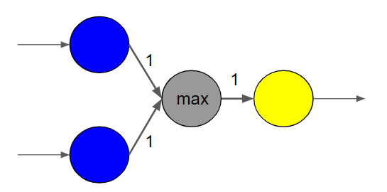
Figure 1: Example of a network where one must replace the max-pooling neuron to compute the path-norm with a single forward pass as in Equation 4.

Proof of Theorem A.1.

Figure 1 shows that Equation 4 is false if the $*$-max-pooling neurons have not been replaced with identity ones as the forward pass yields $1$ while the path-norm is $2$.

We now establish Equation 4. Denote $\mathcal{P}^{\to v}$ the set of paths of $\tilde{G}$ ending at a given neuron $v$. Denote by $\Phi^{\tilde{G}}$ and $a^{\tilde{G}}$ the path-embedding and the path-activations associated with ${\tilde{G}}$. According to Lemma A.1, it holds for every output neuron of $\tilde{G}$

$$(R^{\tilde{G}}_{|\tilde{{\bm{\theta}}}|^{q}}(x))_{v}=\sum_{p\in\mathcal{P}^{\to v}}\Phi^{\tilde{G}}_{p}(|\tilde{{\bm{\theta}}}|^{q})a^{\tilde{G}}_{p}(|\tilde{{\bm{\theta}}}|^{q},x)x_{p_{0}}.$$

Since $\tilde{G}$ has only identity or ReLU neurons, and since the parameters $|\tilde{{\bm{\theta}}}|^{q}$ are non-negative, then for every input $x$ with non-negative coordinates, a simple induction on the neurons shows that for every neuron $u$, it holds

$$u(|\tilde{{\bm{\theta}}}|^{q},x)\geqslant 0.$$

Thus, every path $p\in\mathcal{P}^{\tilde{G}}$ is active (recall that $\mathcal{P}^{\tilde{G}}$ is by definition the set of paths of $\tilde{G}$), meaning that $a^{\tilde{G}}_{p}(|\tilde{{\bm{\theta}}}|^{q},x)=1$ for every path $p\in\mathcal{P}^{\tilde{G}}$ and every non-negative input $x$. Moreover, $\Phi^{\tilde{G}}_{p}(|\tilde{{\bm{\theta}}}|^{q})=\left|\tilde{b}_{p_{0}}\prod_{u\to v\in p}{\tilde{{\bm{\theta}}}^{u\to v}}\right|^{q}=|\Phi^{\tilde{G}}_{p}(\tilde{{\bm{\theta}}})|^{q}$. Note that for every $p\in\mathcal{P}^{G}\subset\mathcal{P}^{\tilde{G}}$, it holds $\Phi^{\tilde{G}}_{p}(\tilde{{\bm{\theta}}})=\Phi^{G}_{p}({\bm{\theta}})$. For $p\in\mathcal{P}^{\tilde{G}}\setminus\mathcal{P}^{G}$, it holds $\Phi^{\tilde{G}}_{p}(\tilde{{\bm{\theta}}})=0$ since such a path must start at a linear neuron that come from a $*$-max-pooling neuron of $G$, for which $\tilde{b}_{p_{0}}$ has been set to zero. At the end, we get:

$$\|\operatorname{R}^{\tilde{G}}_{|\tilde{{\bm{\theta}}}|^{q}}({\bf{1}})\|_{1}=\sum_{p\in\mathcal{P}^{\tilde{G}}}|\Phi^{\tilde{G}}_{p}(\tilde{{\bm{\theta}}})|^{q}=\sum_{p\in\mathcal{P}^{G}}|\Phi^{G}_{p}({\bm{\theta}})|^{q}=\|\Phi(\tilde{{\bm{\theta}}})\|_{q}^{q}.$$

∎

Appendix B Relation between path-norms and products of operators’ norms

Feedforward ReLU networks. For simple models of the form $R_{\bm{\theta}}(x)=M_{D}\operatorname{ReLU}(M_{D-1}\dots\operatorname{ReLU}(M_{1}x))$, it is known that $\|\Phi({\bm{\theta}})\|_{q}\leqslant\prod_{d=1}^{D}\|M_{d}\|_{q,\infty}$ (where $\|M\|_{q,\infty}$ is the maximum $L^{q}$ norm of a row of matrix $M$) (Neyshabur et al., 2015, Theorem 5). Theorem B.1 below generalizes this result to the case of an arbitrary DAG (that may include max pooling, average-pooling, skip connections) with biases. The rescaling of ${\bm{\theta}}$ that makes it an equality without changing $R_{\bm{\theta}}$ is given by Algorithm 1.

Algorithm 1. Algorithm 1 rescales ${\bm{\theta}}$ while preserving $R_{\bm{\theta}}$ because for any neuron $u\notin N_{\textrm{in}}\cup N_{\textrm{out}}$, the activation function $\rho_{u}$ is positively homogeneous: $\rho_{u}(\lambda x)=\lambda\rho_{u}(x)$ for every $\lambda>0$. Thus, $\lambda\rho_{u}(\frac{1}{\lambda}x)=\rho_{u}(x)$. Let us also give some more remarks about this algorithm, which is used here for the case of equality, and in the proof of the generalization bound. The first line of the algorithm considers a topological sorting of the neurons, i.e. an order on the neurons such that if $u\to v$ is an edge then $u$ comes before $v$ in this ordering. Such an order always exists (and it can be computed in linear time). Moreover, note that a classical max-pooling neuron $v$ (corresponding to a $k$-max-pooling neurone with $k=1$ and constant incoming weights all equal to one) has not anymore its incoming weights equal to one after rescaling, in general. This has no incidence on the validity of the generalization bound on classical max-pooling neurons: rescaling is only used in the proof to reduce to another representation of the parameters that realize the same function and that is more handy to work with.

Algorithm 1 Normalization of parameters for norm $q\in[1,\infty)$

1:Consider a topological sorting $v_{1},\dots,v_{k}$ of the neurons

2:for $v=v_{1},\dots,v_{k}$ do

3:     if $v\notin N_{\textrm{in}}\cup N_{\textrm{out}}$ then

4:         $\lambda_{v}=\left(\|{{\bm{\theta}}^{\to v}}\|_{q}^{q}+|b_{v}|^{q}\right)^{1/q}$

5:         if $\lambda_{v}=0$ then

6:              ${{\bm{\theta}}^{v\to}}=0$

7:         else

8:              ${{\bm{\theta}}^{\to v}}\leftarrow\frac{1}{\lambda_{v}}\times{{\bm{\theta}}^{\to v}}$ $\triangleright$ normalize incoming weights

9:              $b_{v}\leftarrow\frac{1}{\lambda_{v}}\times b_{v}$ $\triangleright$ normalize bias

10:              ${{\bm{\theta}}^{v\to}}\leftarrow\lambda_{v}\times{{\bm{\theta}}^{v\to}}$ $\triangleright$ rescale outgoing weights to preserve the function $\operatorname{R}_{\bm{\theta}}$               

Coming back to the comparison between the path-norm and the product of operators’ norms, first, we introduce an equivalent of the product of operators’ norms when neurons are not regrouped in layers. Note that for the simple feedforward model as above, it holds $\prod_{d=1}^{D}\|M_{d}\|_{q,\infty}=\max_{\begin{subarray}{c}u_{0}\to\dots\to u_{D},\\ u_{0}\in N_{\textrm{in}}\end{subarray}}\prod_{d=1}^{D}\|{{\bm{\theta}}^{\to u_{d}}}\|_{q}$. Indeed, all the neurons of two consecutive layers are connected, so the product of the maximum of $L^{q}$-norms over layers is also the maximum over all paths of the product of $L^{q}$-norms.

General DAG ReLU network. Consider now the case of a general DAG ReLU network. For practical purposes, we extend the parameters ${\bm{\theta}}$ to input neurons $v$ by setting $b_{v}=1$ and to $*$-max-pooling neurons by setting $b_{v}=0$. Consider for every path $u_{0}\to\dots\to u_{D}$ the quantity

$$\Pi_{q}(u_{0}\to\dots\to u_{D}):=\left(\sum_{d=0}^{D}\left|b_{u_{d}}\right|^{q}\prod_{k=d+1}^{D}\|{{\bm{\theta}}^{\to u_{k}}}\|_{q}^{q}\right)^{1/q},$$

with the convention that an empty product is equal to one. Note that when there are no biases, it holds $\Pi_{q}(u_{0}\to\dots\to u_{D})=\prod_{d=1}^{D}\|{{\bm{\theta}}^{\to u_{d}}}\|_{q}$, and taking the maximum of this product over all paths $u_{0}\to\dots\to u_{D}$ recovers $\prod_{d=1}^{D}\|M_{d}\|_{q,\infty}$. The next theorem shows that the $L^{q}$ path-norm is the minimum of this complexity measure over all possible rescalings of the parameters ${\bm{\theta}}$ that leave invariant the associated function $R_{\bm{\theta}}$.

Theorem B.1.

For every parameters ${\bm{\theta}}$,

$$\|\Phi({\bm{\theta}})\|_{q}\leqslant\left(\sum_{v\in N_{\textrm{out}}}|b_{v}|^{q}+\|{{\bm{\theta}}^{\to v}}\|_{q}^{q}\max\limits_{\begin{subarray}{c}D\geqslant 0,\\ v\in N_{\textrm{out}},\\ u_{0}\in N_{\textrm{in}},\\ u_{0}\to\dots\to u_{D}\to v\end{subarray}}\Pi_{q}(u_{0}\to\dots\to u_{D})^{q}\right)^{1/q}.$$

If ${\bm{\theta}}$ has been normalized by Algorithm 1, then this is an equality with the maximum being equal to one so that it simply holds $\|\Phi({\bm{\theta}})\|_{q}=\left(\sum_{v\in N_{\textrm{out}}}|b_{v}|^{q}+\|{{\bm{\theta}}^{\to v}}\|_{q}^{q}\right)^{1/q}$.

Figure 2: A network for which the path-norm is zero while the product of operators’ norms scales as $M^{2}$.

Proof of Theorem B.1.

Since $\Phi({\bm{\theta}})=\left(\Phi^{\to v}({\bm{\theta}})\right)_{v\in N_{\textrm{out}}}$, it holds

$$\|\Phi({\bm{\theta}})\|_{q}^{q}=\sum_{v\in N_{\textrm{out}}}\|\Phi^{\to v}({\bm{\theta}})\|_{q}^{q}.$$

For any neuron $v\in N_{\textrm{out}}$, $\Phi^{\to v}({\bm{\theta}})=\left(\begin{array}[]{c}({{\bm{\theta}}^{u\to v}}\Phi^{\to u}({\bm{\theta}}))_{u\in\operatorname{ant}(v)}\\ b_{v}\end{array}\right)$ so that

$$\|\Phi^{\to v}({\bm{\theta}})\|_{q}^{q}=|b_{v}|^{q}+\sum_{u\in\operatorname{ant}(v)}|{{\bm{\theta}}^{u\to v}}|^{q}\|\Phi^{\to u}({\bm{\theta}})\|_{q}^{q}\leqslant|b_{v}|^{q}+\|{{\bm{\theta}}^{\to v}}\|_{q}^{q}\max_{u\in\operatorname{ant}(v)}\|\Phi^{\to u}({\bm{\theta}})\|_{q}^{q}.$$

For every $u\in\operatorname{ant}(v)$, $u$ cannot be an output neuron since it has at least $v$ as a successor. Thus Lemma B.2 gives:

$$\|\Phi^{\to u}({\bm{\theta}})\|_{q}\leqslant\max\limits_{\begin{subarray}{c}D\geqslant 0,\\ u_{0}\in N_{\textrm{in}},\\ u_{0}\to\dots\to u_{D}\to u\end{subarray}}\Pi_{q}(u_{0}\to\dots\to u_{D}\to u).$$

Putting everything together shows the upper-bound:

$$\|\Phi({\bm{\theta}})\|_{q}^{q} \leqslant\left(\sum_{v\in N_{\textrm{out}}}|b_{v}|^{q}\right)+\left(\sum_{v\in N_{\textrm{out}}}\|{{\bm{\theta}}^{\to v}}\|_{q}^{q}\right)\max\limits_{\begin{subarray}{c}D\geqslant 0,\\ v\in N_{\textrm{out}},\\ u_{0}\in N_{\textrm{in}},\\ u_{0}\to\dots\to u_{D}\to v\end{subarray}}(\Pi_{q}(u_{0}\to\dots\to u_{D}))^{q}.$$

We now prove the case of equality. Recall that

$$\|\Phi({\bm{\theta}})\|_{q}^{q} =\sum_{v\in N_{\textrm{out}}}\|\Phi^{\to v}({\bm{\theta}})\|_{q}^{q}$$

$$=\sum_{v\in N_{\textrm{out}}}|b_{v}|^{q}+\sum_{u\in\operatorname{ant}(v)}|{{\bm{\theta}}^{u\to v}}|^{q}\|\Phi^{\to u}({\bm{\theta}})\|_{q}^{q}$$

It would then be sufficient to prove that, as soon as the parameters ${\bm{\theta}}$ have been rescaled with Algorithm 1, then $|{{\bm{\theta}}^{u\to v}}|\|\Phi^{\to u}({\bm{\theta}})\|_{q}=|{{\bm{\theta}}^{u\to v}}|$ for every $v\in N_{\textrm{out}}$ and $u\in\operatorname{ant}(v)$. Indeed, we would then deduce the claim by writing:

$$\|\Phi({\bm{\theta}})\|_{q}^{q} =\sum_{v\in N_{\textrm{out}}}|b_{v}|^{q}+\sum_{u\in\operatorname{ant}(v)}|{{\bm{\theta}}^{u\to v}}|^{q}$$

$$=\sum_{v\in N_{\textrm{out}}}|b_{v}|^{q}+\|{{\bm{\theta}}^{\to v}}\|_{q}^{q}.$$

It now remains to see that $|{{\bm{\theta}}^{u\to v}}|\|\Phi^{\to u}({\bm{\theta}})\|_{q}=|{{\bm{\theta}}^{u\to v}}|$ is a direct consequence of the next lemma.

Lemma B.1.

Consider $u\in N$ and parameters ${\bm{\theta}}$ rescaled by Algorithm 1. If $\|\Phi^{\to u}({\bm{\theta}})\|_{q}=0$ then ${{\bm{\theta}}^{u\to}}=0$. Otherwise, $\|\Phi^{\to u}({\bm{\theta}})\|_{q}=1$.

Proof of Lemma B.1.

The proof is by induction on the neurons. Consider $u\in N_{\textrm{in}}$. Then by convention $\Phi^{\to u}({\bm{\theta}})=1$ so the claim holds true.

Consider now $u\notin N_{\textrm{in}}$ and assume the claim to be true for every antecedent of $u$. It holds:

$$\|\Phi^{\to u}({\bm{\theta}})\|_{q}^{q}=|b_{u}|^{q}+\sum_{w\in\operatorname{ant}(u)}|{{\bm{\theta}}^{w\to u}}|^{q}\|\Phi^{\to w}({\bm{\theta}})\|_{q}^{q}.$$

A consequence of the induction hypothesis is that $|{{\bm{\theta}}^{w\to u}}|^{q}\|\Phi^{\to w}({\bm{\theta}})\|_{q}^{q}=|{{\bm{\theta}}^{w\to u}}|^{q}$ for every $w\in\operatorname{ant}(u)$. Thus

$$\|\Phi^{\to u}({\bm{\theta}})\|_{q}^{q} =|b_{u}|^{q}+\sum_{w\in\operatorname{ant}(u)}|{{\bm{\theta}}^{w\to u}}|^{q}$$

$$=|b_{u}|^{q}+\|{{\bm{\theta}}^{\to u}}\|_{q}^{q}.$$

The latter is either equal to $0$ or $1$ by Lemma B.3. Moreover, when it is equal to $0$, this means that in Algorithm 1, $\lambda_{u}=0$ and ${{\bm{\theta}}^{u\to}}=0$ after rescaling since it is set to zero line 6 of Algorithm 1 when $u$ is encountered, and the coordinates of ${{\bm{\theta}}^{u\to}}$ can only be multiplied by scalars in the remaining of the algorithms so that this property stays true for the remaining of the algorithm. This proves the claim for $u$, and thus the induction. ∎

∎

Lemma B.2.

Consider an exponent $q\in[1,\infty)$. For every neuron $v$, it holds

$$\min\limits_{\begin{subarray}{c}D\geqslant 0,\\ u_{0}\in N_{\textrm{in}},\\ u_{0}\to\dots\to u_{D}\to v\end{subarray}}\Pi_{q}(u_{0}\to\dots\to u_{D}\to v)\leqslant\|\Phi^{\to v}({\bm{\theta}})\|_{q}\leqslant\max\limits_{\begin{subarray}{c}D\geqslant 0,\\ u_{0}\in N_{\textrm{in}},\\ u_{0}\to\dots\to u_{D}\to v\end{subarray}}\Pi_{q}(u_{0}\to\dots\to u_{D}\to v),$$

where by convention, an empty minimum (resp. maximum) is $-\infty$ (resp. $\infty$) and where we define by convention $\Phi^{\to u}({\bm{\theta}})={{\bm{\theta}}^{\to v}}=1$ for an input neuron $u\in N_{\textrm{in}}$.

Proof of Lemma B.2.

The proof goes by induction on a topological sorting of the graph. The first neurons of the sorting are the neurons without antecedents, i.e. the input neurons by definition. The inequality is true for such neurons since it writes $-\infty\leqslant 1\leqslant\infty$ by convention. Indeed $\|\Phi^{\to v}({\bm{\theta}})\|_{q}=1$, and the minimum and maximum are empty.

Consider a neuron $v\notin N_{\textrm{in}}$ and assume that this is true for every neuron before $v$ in a topological sorting of the graph. By definition,

$$\Phi^{\to v}({\bm{\theta}})=\left(\begin{array}[]{c}({{\bm{\theta}}^{u\to v}}\Phi^{\to u}({\bm{\theta}}))_{u\in\operatorname{ant}(v)}\\ b_{v}\end{array}\right)$$

so that

$$\|\Phi^{\to v}({\bm{\theta}})\|_{q}^{q}=|b_{v}|^{q}+\sum_{u\in\operatorname{ant}(v)}|{{\bm{\theta}}^{u\to v}}|^{q}\|\Phi^{\to u}({\bm{\theta}})\|_{q}^{q}.$$

Thus

$$|b_{v}|^{q}+\|{{\bm{\theta}}^{\to v}}\|_{q}^{q}\min_{u\in\operatorname{ant}(v)}\|\Phi^{\to u}({\bm{\theta}})\|_{q}^{q}\leqslant\|\Phi^{\to v}({\bm{\theta}})\|_{q}^{q}\leqslant|b_{v}|^{q}+\|{{\bm{\theta}}^{\to v}}\|_{q}^{q}\max_{u\in\operatorname{ant}(v)}\|\Phi^{\to u}({\bm{\theta}})\|_{q}^{q}.$$

Every $u\in\operatorname{ant}(v)$ must arrive before $v$ in the topological sorting so the induction hypothesis applies to them. Thus:

$$\|\Phi^{\to v}({\bm{\theta}})\|_{q}^{q} \leqslant|b_{v}|^{q}+\|{{\bm{\theta}}^{\to v}}\|_{q}^{q}\max_{u\in\operatorname{ant}(v)}\max\limits_{\begin{subarray}{c}D\geqslant 0,\\ u_{0}\in N_{\textrm{in}},\\ u_{0}\to\dots\to u_{D}\to u\end{subarray}}\left(\Pi_{q}(u_{0}\to\dots\to u_{D}\to u)\right)^{q}$$

$$=|b_{v}|^{q}+\|{{\bm{\theta}}^{\to v}}\|_{q}^{q}\max\limits_{\begin{subarray}{c}D\geqslant 1,\\ u_{0}\in N_{\textrm{in}},\\ u_{0}\to\dots\to u_{D}\to v\end{subarray}}\left(\Pi_{q}(u_{0}\to\dots\to u_{D})\right)^{q}$$

Now, note that for any path $u_{0}\to\dots\to u_{D}\to v$, it holds

$$|b_{v}|^{q}+\|{{\bm{\theta}}^{\to v}}\|_{q}^{q}\left(\Pi_{q}(u_{0}\to\dots\to u_{D})\right)^{q}=\left(\Pi_{q}(u_{0}\to\dots\to u_{D}\to v)\right)^{q}.$$

Indeed, denoting $u_{D+1}=v$, it holds by definition

$$|b_{v}|^{q}+\|{{\bm{\theta}}^{\to v}}\|_{q}^{q}\left(\Pi_{q}(u_{0}\to\dots\to u_{D})\right)^{q} =|b_{v}|^{q}\underbrace{\left(\prod_{k=D+2}^{D+1}\|{{\bm{\theta}}^{\to u_{k}}}\|_{q}^{q}\right)}_{=1\textrm{ (empty product)}}+\|{{\bm{\theta}}^{\to v}}\|_{q}^{q}\sum_{d=0}^{D}\left|b_{u_{d}}\right|^{q}\prod_{k=d+1}^{L}\|{{\bm{\theta}}^{\to u_{k}}}\|_{q}^{q}$$

$$=|b_{u_{D+1}}|^{q}\left(\prod_{k=D+2}^{D+1}\|{{\bm{\theta}}^{\to u_{k}}}\|_{q}^{q}\right)+\sum_{d=0}^{D}\left|b_{u_{d}}\right|^{q}\prod_{k=d+1}^{D+1}\|{{\bm{\theta}}^{\to u_{k}}}\|_{q}^{q}$$

$$=\sum_{d=0}^{D+1}\left|b_{u_{d}}\right|^{q}\prod_{k=d+1}^{D+1}\|{{\bm{\theta}}^{\to u_{k}}}\|_{q}^{q}$$

$$=\left(\Pi_{q}(u_{0}\to\dots\to u_{D}\to v)\right)^{q}.$$

Thus

$$\|\Phi^{\to v}({\bm{\theta}})\|_{q}^{q}\leqslant\max\limits_{\begin{subarray}{c}D\geqslant 1,\\ u_{0}\in N_{\textrm{in}},\\ u_{0}\to\dots\to u_{D}\to v\end{subarray}}\left(\Pi_{q}(u_{0}\to\dots\to u_{D}\to v)\right)^{q}$$

and the maximum does not change if we consider $D\geqslant 0$ since any path going from an input neuron to $v$ must be of length at least equal to one because $v$ is not an input neuron itself. This proves that the upper bound by induction, and a similar argument applies for the lower bound. ∎

Lemma B.3.

Consider an exponent $q\in[1,\infty)$. Any output parameters ${\bm{\theta}}$ of Algorithm 1 are normalized, in the sense that for every neuron $v$ which is not an output neuron, it holds:

$$\|{{\bm{\theta}}^{\to v}}\|_{q}^{q}+|b_{v}|^{q}=\left\{\begin{array}[]{cc}0&\textrm{if }\|{{\bm{\theta}}^{\to v}}\|_{q}=b_{v}=0,\\ 1&\textrm{otherwise}.\end{array}\right.$$

Proof of Lemma B.3.

It is clear that the claim holds true right after iteration of line 2 of Algorithm 1 corresponding to $v$. And since the last time the incoming weights and the bias of a neuron $v$ are modified is when this is the turn of $v$ in line 2, then the claim holds true. Indeed, the neurons are seen in an order given by a topological sorting, and given the lines 8, 9 and 10, the incoming weights of $v$ can only be modified when this is the turn of $v$ or one of its antecedents. But the antecedents of $v$ come before $v$ in any topological order, so they are seen before $v$ line 2. Moreover, from line 9, it is clear that the bias of $v$ can only be modified when this is the turn of $v$ line 2. ∎

Appendix C Relevant (and apparently new) contraction lemmas

The main result is Lemma C.1.

Lemma C.1.

Consider finite sets $I,W,Z$, and for each $z\in Z$, consider a set $T^{z}\subset({\mathbb{R}}^{W})^{I}$. We denote $t=(t_{i})_{i\in I}\in T^{z}$ with $t_{i}=(t_{i,w})_{w\in W}\in{\mathbb{R}}^{W}$. Consider functions $f_{i,z}:{\mathbb{R}}^{W}\to{\mathbb{R}}$ and a finite family ${\bm{\varepsilon}}=({\bm{\varepsilon}}_{j})_{j\in J}$ of independent identically distributed Rademacher variables, with the index set $J$ that will be clear from the context. Finally, consider a convex and non-decreasing function $G:{\mathbb{R}}\to{\mathbb{R}}$. Assume that at least one of the following setting holds.

Setting 1: scalar input case. $|W|=1$ and for every $i\in I$ and $z\in Z$, $f_{i,z}$ is $1$-Lipschitz with $f_{i,z}(0)=0$.

Setting 2: $*$-max-pooling case. For every $i\in I$ and $z\in Z$, there is $k_{i,z}\in{\mathbb{N}}_{>0}$ such that for every $t\in T^{z}$, $f_{i,z}(t)=t_{(k_{i,z})}$ is the $k_{i,z}$-th largest coordinate of $t$.

Then:

$${\mathbb{E}}\max_{z\in Z}\sup_{t\in T^{z}}G\left(\sum_{i\in I}{\bm{\varepsilon}}_{i,z}f_{i,z}(t_{i})\right)\leqslant{\mathbb{E}}\max_{z\in Z}\sup_{t\in T^{z}}G\left(\sum_{i\in I,w\in W}{\bm{\varepsilon}}_{i,w,z}t_{i,w}\right).$$ (5)

The scalar input case is a simple application of (Ledoux & Talagrand, 1991, Theorem 4.12). Indeed, for $z\in Z$ and $t\in T^{z}$, define $s(z,t)\in{\mathbb{R}}^{I\times Z}$ to be the matrix with coordinates $(i,v)\in I\times Z$ given by $[s(z,t)]_{i,v}=t_{i}$ if $v=z$, $0$ otherwise. Define also $g_{i,v}=f_{i}$. Since $g_{i,v}(0)=0$, it holds:

$$\sum_{i\in I}{\bm{\varepsilon}}_{i,z}f_{i}(t_{i})=\sum_{i\in I,v\in Z}{\bm{\varepsilon}}_{i,v}g_{i,v}([s(z,t)]_{i,v}).$$

If $S:=\{s(z,t),z\in Z,t\in T^{z}\}$ and $J:=I\times Z$ then the result claimed in the scalar case reads

$${\mathbb{E}}\sup_{s\in S}G\left(\sum_{j\in J}{\bm{\varepsilon}}_{j}f_{j}(s_{j})\right)\leqslant{\mathbb{E}}\sup_{s\in S}G\left(\sum_{j\in J}{\bm{\varepsilon}}_{j}s_{j}\right).$$

The latter is true by Theorem 4.12 of Ledoux & Talagrand (1991). We still give an alternative proof below that turns to be useful for the $*$-max-pooling case. This alternative proof actually mimics the scheme of proof of Theorem 4.12 in Ledoux & Talagrand (1991): the beginning of the proof is the same for the scalar case and the $*$-max-pooling case, and then the arguments become specific to each case.

Note that Theorem 4.12 of Ledoux & Talagrand (1991) does not apply for the $*$-max-pooling case because the $t_{i}$’s are now vectors. The most related result we could find is a vector-valued contraction inequality (Maurer, 2016) that is known in the specific case where $|Z|=1$, $G$ is the identity, and for arbitrary $1$-Lipschitz functions $f_{i,z}$ such that $f_{i,z}(0)=0$ (with a different proof, and with a factor $\sqrt{2}$ on the right-hand side). Here, the vector-valued case we are interested in is $f_{i,z}=k_{i,z}\textrm{-}\mathtt{pool}$ and $G=\exp$, which is covered by Lemma C.1. We could not find it stated elsewhere.

In the proof of Lemma C.1, we reduce to the simpler case where $|Z|=1$ and $|I|=1$ that corresponds to the next lemma. Again, the scalar input case is given by (Ledoux & Talagrand, 1991, Equation (4.20)) while the $*$-max-pooling case is apparently new.

Lemma C.2.

Consider a finite set $W$, a set $T$ of elements $t=(t_{1},t_{2})\in{\mathbb{R}}^{W}\times{\mathbb{R}}$ and a function $f:{\mathbb{R}}^{W}\to{\mathbb{R}}$. Consider also a convex non-decreasing function $F:{\mathbb{R}}\to{\mathbb{R}}$ and a family of iid Rademacher variables $({\bm{\varepsilon}}_{j})_{j\in J}$ where $J$ will be clear from the context. Assume that we are in one of the two following situations.

Scalar input case. $f$ is $1$-Lipschitz, satisfies $f(0)=0$ and has a scalar input ($|W|=1$).

$*$-max-pooling case. There is $k\in{\mathbb{N}}_{>0}$ such that $f$ computes the $k$-th largest coordinate of its input.

Denoting $t_{1}=(t_{1,w})_{w\in W}$, then it holds:

$${\mathbb{E}}\sup_{t\in T}F\left({\bm{\varepsilon}}_{1}f(t_{1})+t_{2}\right)\leqslant{\mathbb{E}}\sup_{t\in T}F\left(\sum_{w}{\bm{\varepsilon}}_{1,w}t_{1,w}+t_{2}\right).$$

The proof of Lemma C.2 is postponed. We now prove Lemma C.1.

Proof of Lemma C.1.

First, because of the Lipschitz assumptions on the $f_{i}$’s and the convexity of $G$, everything is measurable and the expectations are well defined.

We prove the result by reducing to the simpler case of Lemma C.2. This is inspired by the reduction done in the proof of (Ledoux & Talagrand, 1991, Theorem 4.12) in the special case of scalar $t_{i}$’s ($|W|=1$).

Reduce to the case $|Z|=1$ by conditioning and iteration.

For $z\in Z$, define

$$A_{z} :=\sup_{t\in T^{z}}G\left(\sum_{i\in I}{\bm{\varepsilon}}_{i,z}f_{i,z}(t_{i})\right),$$

$$B_{z} :=\sup_{t\in T^{z}}G\left(\sum_{i\in I,w\in W}{\bm{\varepsilon}}_{i,w,z}t_{i,w}\right).$$

Lemma C.3 applies since these random variables are independent. Thus, it is enough to prove that for every $c\in[-\infty,\infty)$:

$${\mathbb{E}}\max(A_{z},c)\leqslant{\mathbb{E}}\max(B_{z},c).$$

Define $F(x)=\max(G(x),c)$. This can be rewritten as (inverting the supremum and the maximum)

$${\mathbb{E}}\sup_{t\in T^{z}}F\left(\sum_{i\in I}{\bm{\varepsilon}}_{i,z}f_{i,z}(t_{i})\right)\leqslant{\mathbb{E}}\sup_{t\in T^{z}}F\left(\sum_{i\in I,w\in W}{\bm{\varepsilon}}_{i,w,z}t_{i,w}\right).$$ (6)

We just reduced to the case where there is a single $z$ to consider, up to the price of replacing $G$ by $F$. Since $G$ and $x\to\max(x,c)$ are non-decreasing and convex, then so is $F$ by composition. Alternatively, note that we could also have reduced to the case $|Z|=1$ by defining $S:=\{s(z,t),z\in Z,t\in T^{z}\}$ just as it is done right after the statement of Lemma C.1. In order to apply Lemma C.2, it remains to reduce to the case $|I|=1$.

Reduce to the case $|I|=1$ by conditioning and iteration. Lemma C.4 shows that in order to prove Equation 6, it is enough to prove that for every $i\in I$ and every subset $R\subset{\mathbb{R}}^{W}\times R$, denoting $r=(r_{1},r_{2})\in{\mathbb{R}}^{W}\times{\mathbb{R}}$, it holds

$${\mathbb{E}}\sup_{r\in R}F\left({\bm{\varepsilon}}_{i,z}f_{i,z}(r_{1})+r_{2}\right)\leqslant{\mathbb{E}}\sup_{r\in R}F\left(\sum_{w\in W}{\bm{\varepsilon}}_{i,w,z}r_{1,w}+r_{2}\right).$$

We just reduced to the case $|I|=1$ since one can now consider the indices $i$ one by one. The latter inequality is now a direct consequence of Lemma C.2. This proves the result. ∎

Lemma C.3.

Consider a finite set $Z$ and independent families of independent real random variables $(A_{z})_{z\in Z}$ and $(B_{z})_{z\in Z}$. If for every $z\in Z$ and every constant $c\in[-\infty,\infty)$, it holds ${\mathbb{E}}\max(A_{z},c)\leqslant{\mathbb{E}}\max(B_{z},c)$ then

$${\mathbb{E}}\max_{z\in Z}A_{z}\leqslant{\mathbb{E}}\max_{z\in Z}B_{z}.$$

Proof of Lemma C.3.

The proof is by conditioning and iteration. To prove the result, it is enough to prove that if

$${\mathbb{E}}\max_{z\in Z}A_{z}\leqslant{\mathbb{E}}\max\left(\max_{z\in Z_{1}}A_{z},\max_{z\in Z_{2}}B_{z}\right)$$

for some partition $Z_{1},Z_{2}$ of $Z$, with $Z_{2}$ possibly empty for the initialization of the induction, then for every $z_{0}\in Z_{1}$:

$${\mathbb{E}}\max_{z\in Z}A_{z}\leqslant{\mathbb{E}}\max\left(\max_{z\in Z_{1}\setminus\{z_{0}\}}A_{z},\max_{z\in Z_{2}\cup\{z_{0}\}}B_{z}\right),$$

with the convention that the maximum over an empty set is $-\infty$. Indeed, the claim would then come directly by induction on the size of $Z_{2}$.

Now, consider an arbitrary partition $Z_{1},Z_{2}$ of $Z$, with $Z_{2}$ possibly empty, and consider $z_{0}\in Z_{1}$. It is then enough to prove that

$${\mathbb{E}}\max\left(\max_{z\in Z_{1}}A_{z},\max_{z\in Z_{2}}B_{z}\right)\leqslant{\mathbb{E}}\max\left(\max_{z\in Z_{1}\setminus\{z_{0}\}}A_{z},\max_{z\in Z_{2}\cup\{z_{0}\}}B_{z}\right).$$ (7)

Define the random variable $C=\max\left(\max_{z\in Z_{1}\setminus\{z_{0}\}}A_{z},\max_{z\in Z_{2}}B_{z}\right)$ which may be equal to $-\infty$ when the maximum is over empty sets, and which is independent of $A_{z_{0}}$ and $B_{z_{0}}$. Then:

$$\max\left(\max_{z\in Z_{1}}A_{z},\max_{z\in Z_{2}}B_{z}\right)=\max\left(A_{z_{0}},C\right)$$

and

$$\max\left(\max_{z\in Z_{1}\setminus\{z_{0}\}}A_{z},\max_{z\in Z_{2}\cup\{z_{0}\}}B_{z}\right)=\max\left(B_{z_{0}},C\right).$$

Equation 7 is then equivalent to

$${\mathbb{E}}\max(A_{z_{0}},C)\leqslant{\mathbb{E}}\max(B_{z_{0}},C)$$

with $C$ independent of $A_{z_{0}}$ and $B_{z_{0}}$. For a constant $c\in[-\infty,\infty)$, denote $A(c)={\mathbb{E}}\max(A_{z_{0}},c)$ and $B(c)={\mathbb{E}}\max(B_{z_{0}},c)$. Then:

$${\mathbb{E}}\max(A_{z_{0}},C) ={\mathbb{E}}\left({\mathbb{E}}\left(\max\left(A_{z_{0}},C\right)|A_{z_{0}}\right)\right)$$ law of total expectation

$$={\mathbb{E}}A(C) \text{independence of $C$ and $A_{z_{0}}$}.$$

and similarly ${\mathbb{E}}\max(B_{z_{0}},C)={\mathbb{E}}B(C)$. It is then enough to prove that $A(C)\leqslant B(C)$ almost surely. Since $C\in[-\infty,\infty)$, this is true by assumption. This proves the claims. ∎

Lemma C.4.

Consider finite sets $I,W$ and independent families of independent real random variables $({\bm{\varepsilon}}_{i})_{i\in I}$ and $({\bm{\varepsilon}}_{i,w})_{i\in I,w\in W}$. Consider functions $f_{i}:{\mathbb{R}}^{W}\to{\mathbb{R}}$ and $F:{\mathbb{R}}\to{\mathbb{R}}$ that are continuous. Assume that for every $i\in I$ and every subset $R\subset{\mathbb{R}}^{W}\times{\mathbb{R}}$, denoting $r=(r_{1},r_{2})\in R$ with $r_{1}=(r_{1,w})_{w}\in{\mathbb{R}}^{W}$ and $r_{2}\in{\mathbb{R}}$ the components of $r$, it holds

$${\mathbb{E}}\sup_{r\in R}F({\bm{\varepsilon}}_{i}f_{i}(r_{1})+r_{2})\leqslant{\mathbb{E}}\sup_{r\in R}F(\sum_{w\in W}{\bm{\varepsilon}}_{i,w}r_{1,w}+r_{2}).$$

Consider an arbitrary $T\subset({\mathbb{R}}^{W})^{I}$ and for $t=(t_{i})_{i\in I}\in T$, denote $t_{i,w}$ the $w$-th coordinate of $t_{i}\in{\mathbb{R}}^{W}$. Then

$${\mathbb{E}}\sup_{t\in T}F(\sum_{i\in I}{\bm{\varepsilon}}_{i}f_{i}(t_{i}))\leqslant{\mathbb{E}}\sup_{t\in T}F(\sum_{i\in I,w\in W}{\bm{\varepsilon}}_{i,w}t_{i,w}).$$

Proof of Lemma C.4.

The continuity assumption on $F$ and the $f_{i}$’s is only used to make all the considered suprema measurable. The proof goes by conditioning and iteration. For any $J\subset I$, denote ${\bm{\varepsilon}}_{J}$ the family that contains both $({\bm{\varepsilon}}_{j})_{j\in J}$ and $({\bm{\varepsilon}}_{j,w})_{j\in J,w\in W}$. Define

$$h_{J}(t,{\bm{\varepsilon}}_{J}) :=\sum_{j\in J}{\bm{\varepsilon}}_{j}f_{j}(t_{j}),$$

$$H_{J}(t,{\bm{\varepsilon}}_{J}) :=\sum_{j\in J,w\in W}{\bm{\varepsilon}}_{j,w}t_{j,w},$$

with the convention that an empty sum is zero. To make notations lighter, if $J=\{j\}$ then we may write $h_{j}$ and $H_{j}$ instead of $h_{J}$ and $H_{J}$. We also omit to write the dependence on ${\bm{\varepsilon}}_{J}$ as soon as possible. What we want to prove is thus equivalent to

$${\mathbb{E}}\sup_{t\in T}F(h_{I}(t))\leqslant{\mathbb{E}}\sup_{t\in T}F(H_{I}(t)).$$

It is enough to prove that for every partition $I_{1},I_{2}$ of $I$, with $I_{2}$ possibly empty, if

$${\mathbb{E}}\sup_{t\in T}F(h_{I}(t))\leqslant{\mathbb{E}}\sup_{t\in T}F(h_{I_{1}}(t)+H_{I_{2}}(t)),$$

then for every $j\in I_{1}$,

$${\mathbb{E}}\sup_{t\in T}F(h_{I}(t))\leqslant{\mathbb{E}}\sup_{t\in T}F(h_{I_{1}\setminus\{j\}}(t)+H_{I_{2}\cup\{j\}}(t)).$$

Indeed, the result would then come by induction on the size of $I_{2}$. Fix an arbitrary partition $I_{1},I_{2}$ of $I$ with $I_{2}$ possibly empty, and $j\in I_{1}$. It is then enough to prove that

$${\mathbb{E}}\sup_{t\in T}F(h_{I_{1}}(t)+H_{I_{2}}(t))\leqslant{\mathbb{E}}\sup_{t\in T}F(h_{I_{1}\setminus\{j\}}(t)+H_{I_{2}\cup\{j\}}(t)).$$ (8)

Denote ${\bm{\varepsilon}}_{-j}:={\bm{\varepsilon}}_{I\setminus\{j\}}$ and ${\varphi}(t,{\bm{\varepsilon}}_{-j}):=h_{I_{1}\setminus\{j\}}(t,{\bm{\varepsilon}}_{I_{1}\setminus\{j\}})+H_{I_{2}}(t,{\bm{\varepsilon}}_{I_{2}}))$. It holds:

$$h_{I_{1}}(t)+H_{I_{2}}(t)=h_{j}(t,{\bm{\varepsilon}}_{j})+{\varphi}(t,{\bm{\varepsilon}}_{-j})$$

and, writing ${\bm{\varepsilon}}_{j,\cdot}=({\bm{\varepsilon}}_{j,w})_{w\in W}$:

$$h_{I_{1}\setminus\{j\}}(t)+H_{I_{2}\cup\{j\}}(t)=H_{j}(t,{\bm{\varepsilon}}_{j,\cdot})+{\varphi}(t,{\bm{\varepsilon}}_{-j}).$$

Consider the measurable functions

$$g({\bm{\varepsilon}}_{j},{\bm{\varepsilon}}_{-j}):=\sup_{t\in T}F(h_{j}(t,{\bm{\varepsilon}}_{j})+{\varphi}(t,{\bm{\varepsilon}}_{-j}))$$

and

$$G({\bm{\varepsilon}}_{j,\cdot},{\bm{\varepsilon}}_{-j}):=\sup_{t\in T}F(H_{j}(t,{\bm{\varepsilon}}_{j,\cdot})+{\varphi}(t,{\bm{\varepsilon}}_{-j})).$$

Denote $\Delta$ the ambiant space of ${\bm{\varepsilon}}_{-j}$ and consider a constant $\delta\in\Delta$. Define $\hat{g}(\delta)={\mathbb{E}}g({\bm{\varepsilon}}_{j},\delta)$ and $\hat{G}(\delta)={\mathbb{E}}G({\bm{\varepsilon}}_{j,\cdot},\delta)$. Then

$${\mathbb{E}}\sup_{t\in T}F(h_{I_{1}}(t)+H_{I_{2}}(t)) ={\mathbb{E}}g({\bm{\varepsilon}}_{j},{\bm{\varepsilon}}_{-j}) g$$ by definition of

$$={\mathbb{E}}\left({\mathbb{E}}\left(g({\bm{\varepsilon}}_{j},{\bm{\varepsilon}}_{-j})|{\bm{\varepsilon}}_{-j}\right)\right)$$ law of total expectation

$$={\mathbb{E}}\hat{g}({\bm{\varepsilon}}_{-j}) {\bm{\varepsilon}}_{j} {\bm{\varepsilon}}_{-j}$$ independence of and

and similarly ${\mathbb{E}}\sup_{t\in T}F(h_{I_{1}\setminus\{j\}}(t)+H_{I_{2}\cup\{j\}}(t))={\mathbb{E}}\hat{G}({\bm{\varepsilon}}_{-j})$. Thus, Equation 8 is equivalent to ${\mathbb{E}}\hat{g}({\bm{\varepsilon}}_{-j})\leqslant{\mathbb{E}}\hat{G}({\bm{\varepsilon}}_{-j})$. For every $\delta\in\Delta$, we can define $R(\delta)=\{(t_{j},{\varphi}(t,\delta))\in{\mathbb{R}}^{W}\times{\mathbb{R}},t\in T\}$ and it holds

$$\hat{g}(\delta)={\mathbb{E}}\sup_{r\in R}F({\bm{\varepsilon}}_{j}f_{j}(r_{1})+r_{2})$$

and

$$\hat{G}(\delta)={\mathbb{E}}\sup_{r\in R}F(\sum_{w\in}{\bm{\varepsilon}}_{j,w}r_{1,w}+r_{2}).$$

Thus, $\hat{g}(\delta)\leqslant\hat{G}(\delta)$ for every $\delta\in\Delta$ by assumption. This shows the claim. ∎

Proof of Lemma C.2.

Recall that we want to prove

$${\mathbb{E}}\sup_{t\in T}F\left({\bm{\varepsilon}}_{1}f(t_{1})+t_{2}\right)\leqslant{\mathbb{E}}\sup_{t\in T}F\left(\sum_{w\in W}{\bm{\varepsilon}}_{1,w}t_{1,w}+t_{2}\right).$$ (9)

Scalar input case. In this case, $|W|=1$ i.e. the inputs $t_{1}$ are scalar and the result is well-known, see (Ledoux & Talagrand, 1991, Equation (4.20)).

$k$-max-pooling case. In this case, $f$ computes the $k$-th largest coordinate of its input. Computing explicitly the expectation where the only random thing is ${\bm{\varepsilon}}_{1}\in\{-1,1\}$, the left-hand side of Equation 9 is equal to

$$\frac{1}{2}\sup_{t\in T}F\left(f(t_{1})+t_{2}\right)+\frac{1}{2}\sup_{s\in T}F\left(-f(s_{1})+s_{2}\right).$$

Consider $s,t\in T$. Recall that $s_{1},t_{1}\in{\mathbb{R}}^{W}$. Denote $s_{1,(k)}$ the $k$-th largest component of vector $s_{1}$. The set $\{w\in W:s_{1,w}\leqslant s_{1,(k)}\}$ has at least $|W|-k+1$ elements, and $\{w\in W:t_{1,(k)}\leqslant t_{1,w}\}$ has at least $k$ elements, so their intersection is not empty. Consider any $w(s,t)$ in this intersection. We are now going to use that both $f(t_{1})=t_{1,(k)}\leqslant t_{1,w(s,t)}$ and $-f(s_{1})=-s_{1,(k)}\leqslant-s_{1,w(s,t)}$. Even if we are not going to use it, note that this implies $f(t)-f(s)\leqslant t_{1,w(s,t)}-s_{1,w(s,t)}$: we are exactly using an argument that establishes that $f$ is $1$-Lipschitz. Since $f(t_{1})=t_{1,(k)}\leqslant t_{1,w(s,t)}$ and $F$ is non-decreasing, it holds:

$$F\left(f(t_{1})+t_{2}\right)\leqslant F\left(t_{1,w(s,t)}+t_{2}\right)$$

$$\underset{{\bm{\varepsilon}}\textrm{ centered}}{=} F\left(t_{1,w(s,t)}+{\mathbb{E}}\left(\sum_{w\neq w(s,t)}{\bm{\varepsilon}}_{1,w}t_{1,w}\right)+t_{2}\right)$$

$$\underset{\textrm{Jensen}}{\leqslant} {\mathbb{E}}F\left(t_{1,w(s,t)}+\sum_{w\neq w(s,t)}{\bm{\varepsilon}}_{1,w}t_{1,w}+t_{2}\right).$$

Moreover, $-f(s_{1})=-s_{1,(k)}\leqslant-s_{1,w(s,t)}$ so that in a similar way:

$$F\left(-f(s_{1})+s_{2}\right)\leqslant F\left(-s_{1,w(s,t)}+s_{2}\right)$$

$$\leqslant F\left(-s_{1,w(s,t)}+{\mathbb{E}}\left(\sum_{w\neq w(s,t)}{\bm{\varepsilon}}_{1,w}s_{1,w}\right)+s_{2}\right)$$

$$\leqslant {\mathbb{E}}F\left(-s_{1,w(s,t)}+\sum_{w\neq w(s,t)}{\bm{\varepsilon}}_{1,w}s_{1,w}+s_{2}\right).$$

At the end, we get

$$\frac{1}{2}F\left(f(t_{1})+t_{2}\right)+\frac{1}{2}F\left(-f(s_{1})+s_{2}\right)$$

$$\leqslant\frac{1}{2}{\mathbb{E}}F\left(t_{1,w(s,t)}+\sum_{w\neq w(s,t)}{\bm{\varepsilon}}_{1,w}t_{1,w}+t_{2}\right)$$

$$+\frac{1}{2}{\mathbb{E}}F\left(-s_{1,w(s,t)}+\sum_{w\neq w(s,t)}{\bm{\varepsilon}}_{1,w}s_{1,w}+s_{2}\right)$$

$$\leqslant\frac{1}{2}{\mathbb{E}}\sup_{r\in T}F\left(r_{1,w(s,t)}+\sum_{w\neq w(s,t)}{\bm{\varepsilon}}_{1,w}r_{1,w}+r_{2}\right)$$

$$+\frac{1}{2}{\mathbb{E}}\sup_{r\in T}F\left(-r_{1,w(s,t)}+\sum_{w\neq w(s,t)}{\bm{\varepsilon}}_{1,w}r_{1,w}+r_{2}\right)$$

$$={\mathbb{E}}\sup_{r\in T}F\left({\bm{\varepsilon}}_{1,w(s,t)}r_{1,w(s,t)}+\sum_{w\neq w(s,t)}{\bm{\varepsilon}}_{1,w}r_{1,w}+r_{2}\right)$$

$$={\mathbb{E}}\sup_{r\in T}F\left(\sum_{w}{\bm{\varepsilon}}_{1,w}r_{1,w}+r_{2}\right).$$

The latter is independent of $s,t$. Taking the supremum over all $s,t\in T$ yields Equation 9 and thus the claim. ∎

Appendix D Peeling argument

First, we state a simple lemma that will be used several times.

Lemma D.1.

Consider a vector ${\bm{\varepsilon}}\in{\mathbb{R}}^{n}$ with iid Rademacher coordinates, meaning that ${\mathbb{P}}({\bm{\varepsilon}}_{i}=1)={\mathbb{P}}({\bm{\varepsilon}}_{i}=-1)=1/2$. Consider a function $G:{\mathbb{R}}\to{\mathbb{R}}_{\geqslant 0}$. Consider a set $X\subset{\mathbb{R}}^{n}$. Then whenever the suprema are measurable:

$${\mathbb{E}}_{\bm{\varepsilon}}\sup_{x\in X}G\left(\left|\sum_{i=1}^{n}{\bm{\varepsilon}}_{i}x_{i}\right|\right)\leqslant 2{\mathbb{E}}_{\bm{\varepsilon}}\sup_{x\in X}G\left(\sum_{i=1}^{n}{\bm{\varepsilon}}_{i}x_{i}\right).$$

Proof of Lemma D.1.

Since $G\geqslant 0$, it holds $G(|x|)\leqslant G(x)+G(-x)$. Thus

$${\mathbb{E}}_{\bm{\varepsilon}}\sup_{x\in X}G\left(\left|\sum_{i=1}^{n}{\bm{\varepsilon}}_{i}x_{i}\right|\right)\leqslant{\mathbb{E}}_{\bm{\varepsilon}}\sup_{x\in X}G\left(\sum_{i=1}^{n}{\bm{\varepsilon}}_{i}x_{i}\right)+{\mathbb{E}}_{\bm{\varepsilon}}\sup_{x\in X}G\left(\sum_{i=1}^{n}(-{\bm{\varepsilon}}_{i})x_{i}\right).$$

Since ${\bm{\varepsilon}}$ is symmetric, that is $-{\bm{\varepsilon}}$ has the same distribution as ${\bm{\varepsilon}}$, then the latter is just $2{\mathbb{E}}_{\bm{\varepsilon}}\sup_{x\in X}G\left(\sum_{i=1}^{n}{\bm{\varepsilon}}_{i}x_{i}\right)$. This proves the claim. ∎

Notations We now fix for all the next results of this section $n$ vectors $x_{1},\dots,x_{n}\in{\mathbb{R}}^{d_{\textrm{in}}}$, for some ${d_{\textrm{in}}}\in{\mathbb{N}}_{>0}$. We denote $x_{i,u}$ the coordinate $u$ of $x_{i}$.

For any neural network architecture, recall that $v({\bm{\theta}},x)$ is the output of neuron $v$ for parameters ${\bm{\theta}}$ and input $x$, and $\operatorname{ant}^{d}(v)$ is the set of neurons $u$ for which there exists a path from $u$ to $v$ of distance $d$. For a set of neurons $V$, denote $R_{V}({\bm{\theta}},x)=(v({\bm{\theta}},x))_{v\in V}$.

Introduction to peeling This section shows that some expected sum over output neurons $v$ can be reduced to an expected maximum over $\operatorname{ant}(v)$, and iteratively over an expected maximum over $\operatorname{ant}^{d}(v)$ for increasing $d$’s. Eventually, the maximum is only over input neurons as soon as $d$ is large enough. We start with the next lemma which is the initialization of the induction over $d$: it peels off the output neurons $v$ to reduce to their antecedents $\operatorname{ant}(v)$.

Lemma D.2.

Consider a neural network architecture as in Definition 2.1 with an associated set $\bm{\Theta}$ of parameters ${\bm{\theta}}$ such that $\sum\limits_{v\in N_{\textrm{out}}}\|{{\bm{\theta}}^{\to v}}\|_{1}+|b_{v}|\leqslant r$. Consider a family of independent Rademacher variables $({\bm{\varepsilon}}_{j})_{j\in J}$ with $J$ that will be clear from the context. Consider a non-decreasing function $G:{\mathbb{R}}\to{\mathbb{R}}_{\geqslant 0}$. Consider a new neuron $b$ (for bias) and set by convention $x_{b}=1$ for every input $x$. Then

$${\mathbb{E}}_{{\bm{\varepsilon}}}G\left(\sup\limits_{{\bm{\theta}}\in\bm{\Theta}}\sum_{\begin{subarray}{c}i=1,\dots,n,\\ v\in N_{\textrm{out}}\end{subarray}}{\bm{\varepsilon}}_{i,v}v({\bm{\theta}},x_{i})\right)\\ \leqslant{\mathbb{E}}_{{\bm{\varepsilon}}}G\left(r\max_{v\in N_{\textrm{out}}}\max_{u\in(\operatorname{ant}(v)\cap N_{\textrm{in}})\cup\{b\}}\left|\sum_{i=1}^{n}{\bm{\varepsilon}}_{i,v}x_{i,u}\right|\right)\\ +{\mathbb{E}}_{{\bm{\varepsilon}}}G\left(r\max_{v\in N_{\textrm{out}}}\max_{u\in\operatorname{ant}(v)\setminus N_{\textrm{in}}}\sup\limits_{{\bm{\theta}}}\left|\sum_{i=1}^{n}{\bm{\varepsilon}}_{i,v}u({\bm{\theta}},x_{i})\right|\right)$$

Proof of Lemma D.2.

Recall that for a set of neurons $V$, we denote $R_{V}({\bm{\theta}},x)=(v({\bm{\theta}},x))_{v\in V}$. Recall that by Definition 2.1, output neurons are identity neurons so that for every $v\in N_{\textrm{out}}$, ${\bm{\theta}}\in\bm{\Theta}$ and every input $x$:

$$v({\bm{\theta}},x)=\left\langle\left(\begin{array}[]{c}{{\bm{\theta}}^{\to v}}\\ b_{v}\end{array}\right),\left(\begin{array}[]{c}R_{\operatorname{ant}(v)}({\bm{\theta}},x)\\ 1\end{array}\right)\right\rangle.$$

Overloading the symbol $b$ to make it represent a new neuron that computes the constant function equal to one ($b({\bm{\theta}},x)=1$), we get:

$${\mathbb{E}}_{{\bm{\varepsilon}}}G\left(\sup\limits_{{\bm{\theta}}}\sum\limits_{\begin{subarray}{c}i=1,\dots,n\\ v\in N_{\textrm{out}}\end{subarray}}{\bm{\varepsilon}}_{i,v}v({\bm{\theta}},x_{i})\right)$$

$$={\mathbb{E}}_{{\bm{\varepsilon}}}G\left(\sup\limits_{{\bm{\theta}}}\sum\limits_{v\in N_{\textrm{out}}}\left\langle\left(\begin{array}[]{c}{{\bm{\theta}}^{\to v}}\\ b_{v}\end{array}\right),\sum_{i=1}^{n}{\bm{\varepsilon}}_{i,v}\left(\begin{array}[]{c}R_{\operatorname{ant}(v)}({\bm{\theta}},x_{i})\\ 1\end{array}\right)\right\rangle\right)$$

$$\underset{\textrm{Hölder}}{\leqslant}{\mathbb{E}}_{{\bm{\varepsilon}}}G\left(\sup\limits_{{\bm{\theta}}}\underbrace{\left(\sum\limits_{v\in N_{\textrm{out}}}\|{{\bm{\theta}}^{\to v}}\|_{1}+|b_{v}|\right)}_{\leqslant r\textrm{ by assumption}}\max_{v\in N_{\textrm{out}}}\left(\left|\sum_{i=1}^{n}{\bm{\varepsilon}}_{i,v}\right|,\max_{u\in\operatorname{ant}(v)}\left|\sum_{i=1}^{n}{\bm{\varepsilon}}_{i,v}u({\bm{\theta}},x_{i})\right|\right)\right)$$

$$\leqslant{\mathbb{E}}_{{\bm{\varepsilon}}}G\left(r\max_{v\in N_{\textrm{out}}}\max_{u\in\operatorname{ant}(v)\cup\{b\}}\sup\limits_{{\bm{\theta}}}\left|\sum_{i=1}^{n}{\bm{\varepsilon}}_{i,v}u({\bm{\theta}},x_{i})\right|\right).$$

Everything is non-negative so the maximum over $u\in\operatorname{ant}(v)\cup\{b\}$ is smaller than the sum of the maxima over $u\in(\operatorname{ant}(v)\cap N_{\textrm{in}})\cup\{b\}$ and $u\in\operatorname{ant}(v)\setminus N_{\textrm{in}}$. Note that when $u$ is an input neuron, it simply holds $u({\bm{\theta}},x_{i})=x_{i,u}$. This proves the result. ∎

We now show how to peel neurons to reduce the maximum over $\operatorname{ant}^{d}(v)$ to $\operatorname{ant}^{d+1}(v)$. Later, we will repeat that until the maximum is only on input neurons. Compared to the previous lemma, note the presence of an index $m=1,\dots,M$ in the maxima. This is because after $d$ steps of peeling (when the maximum over $u$ has been reduced to $u\in\operatorname{ant}^{d}(v)$), we will have $M=K^{d-1}$ where $K$ is the kernel size. Indeed, the number of copies indexed by $m$ gets multiplied by $K$ after each peeling step.

Lemma D.3.

Consider a neural network architecture with an associated set $\bm{\Theta}$ of parameters ${\bm{\theta}}$ such that every neuron $v$ that is not an output neuron satisfies $\|{{\bm{\theta}}^{\to v}}\|_{1}+|b_{v}|\leqslant 1$. Consider a family of independent Rademacher variables $({\bm{\varepsilon}}_{j})_{j\in J}$ with $J$ that will be clear from the context. Consider arbitrary $M,d\in{\mathbb{N}}$ and a convex non-decreasing function $G:{\mathbb{R}}\to{\mathbb{R}}_{\geqslant 0}$. Take a symbol $b$ (for bias) which does not correspond to a neuron ($b\notin N$) and set by convention $x_{b}=1$ for every input $x$. Denote $K$ the maximal kernel size of the network (i.e. the maximum of $|\operatorname{ant}(u)|$ over every neuron $u\in N_{*\textrm{-}\mathtt{pool}}$). Define $P:=|\{k\in{\mathbb{N}}_{>0},\exists u\in N_{k\textrm{-}\mathtt{pool}}\}|$ as the number of different types of $*$-max-pooling neurons in $G$. Then:

$${\mathbb{E}}_{{\bm{\varepsilon}}}G\left(\max_{\begin{subarray}{c}v\in N_{\textrm{out}},\\ m=1,\dots,M\end{subarray}}\max_{u\in\operatorname{ant}^{d}(v)\setminus N_{\textrm{in}}}\sup\limits_{{\bm{\theta}}}\left|\sum_{i=1}^{n}{\bm{\varepsilon}}_{i,v,m}u({\bm{\theta}},x_{i})\right|\right)\\ \leqslant(3+2P){\mathbb{E}}_{{\bm{\varepsilon}}}G\left(\max_{\begin{subarray}{c}v\in N_{\textrm{out}},\\ m=1,\dots,KM\end{subarray}}\max_{u\in(\operatorname{ant}^{d+1}(v)\cap N_{\textrm{in}})\cup\{b\}}\left|\sum_{i=1}^{n}{\bm{\varepsilon}}_{i,v,m}x_{i,u}\right|\right)\\ +(3+2P){\mathbb{E}}_{{\bm{\varepsilon}}}G\left(\max_{\begin{subarray}{c}v\in N_{\textrm{out}},\\ m=1,\dots,KM\end{subarray}}\max_{u\in\operatorname{ant}^{d+1}(v)\setminus N_{\textrm{in}}}\sup\limits_{{\bm{\theta}}}\left|\sum_{i=1}^{n}{\bm{\varepsilon}}_{i,v,m}u({\bm{\theta}},x_{i})\right|\right)$$

Proof.

Step 1: split the neurons depending on their activation function. In the term that we want to bound from above, the neurons $u$ compute something of the form $\rho_{u}(\dots)$ where $\rho_{u}$ is the activation associated with $u$ which is $1$-Lipschitz and satisfy $\rho_{u}(0)=0$. The first step of the proof is to get rid of $\rho_{u}$ using a contraction lemma of the type (Ledoux & Talagrand, 1991, Theorem 4.12). However, here, the function $\rho_{u}$ depends on the neuron $u$, what we are taking a maximum over so that classical contraction lemmas do not apply directly. To resolve this first obstacle, we split the neurons according to their activation function. Below, we highlight in blue what is important and/or the changes from one line to another. Denote $N_{\rho}$ the neurons that have $\rho$ as their associated activation function, and the term with a maximum over all $u\in N_{\rho}$ is denoted:

$$e(\rho):={\mathbb{E}}_{{\bm{\varepsilon}}}G\left(\max_{\begin{subarray}{c}v\in N_{\textrm{out}},\\ m=1,\dots,M\end{subarray}}\max_{u\in(\operatorname{ant}^{d}(v)\cap{\color[rgb]{0,0,1}\bm{N_{\rho}}})\setminus N_{\textrm{in}}}\sup\limits_{{\bm{\theta}}}\left|\sum_{i=1}^{n}{\bm{\varepsilon}}_{i,v,m}u({\bm{\theta}},x_{i})\right|\right),$$

with the convention $e(\rho)=0$ if $N_{\rho}$ is empty. This yields a first bound

$${\mathbb{E}}_{{\bm{\varepsilon}}}G\left(\max_{\begin{subarray}{c}v\in N_{\textrm{out}},\\ m=1,\dots,M\end{subarray}}\max_{u\in\operatorname{ant}^{d}(v)\setminus N_{\textrm{in}}}\sup\limits_{{\bm{\theta}}}\left|\sum_{i=1}^{n}{\bm{\varepsilon}}_{i,v,m}u({\bm{\theta}},x_{i})\right|\right)\\ \leqslant e(\operatorname{ReLU})+e(\operatorname*{id})+\sum_{k}e(k\textrm{-}\mathtt{pool})$$

where the sum of the right-hand side is on all the $k\in{\mathbb{N}}_{>0}$ such that there is at least one neuron in $N_{k\textrm{-}\mathtt{pool}}$. Define $E(\rho)$ to be the same thing as $e(\rho)$ but without the absolute values:

$$E(\rho):={\mathbb{E}}_{{\bm{\varepsilon}}}G\left(\max_{\begin{subarray}{c}v\in N_{\textrm{out}},\\ m=1,\dots,M\end{subarray}}\max_{u\in(\operatorname{ant}^{d}(v)\cap{\color[rgb]{0,0,1}\bm{N_{\rho}}})\setminus N_{\textrm{in}}}\sup\limits_{{\bm{\theta}}}\sum_{i=1}^{n}{\bm{\varepsilon}}_{i,v,m}u({\bm{\theta}},x_{i})\right).$$

Then Lemma D.1 gets rid of the absolute values by paying a factor 2:

$$e(\rho)\leqslant 2E(\rho).$$

We now want to bound each $E(\rho)$.

Step 2: get rid of the $*$-max-pooling and ReLU activation functions. Since the maximal kernel size is $K$, any $*$-max-pooling neuron $u$ must have at most $K$ antecedents. When a $*$-max-pooling neuron $u$ has less than $K$ antecedents, we artificially add neurons $w$ to $\operatorname{ant}(u)$ to make it of cardinal $K$, and we set by convention ${{\bm{\theta}}^{w\to u}}=0$. We also fix an arbitrary order on the antecedents of $u$ and write $\operatorname{ant}(u)_{w}$ for the antecedent number $w$, with $R_{\operatorname{ant}(u)_{w}}$ the function associated with this neuron. For a ReLU or $*$-max-pooling neuron $u$, define the pre-activation of $u$ to be

$${\textrm{pre}}_{u}({\bm{\theta}},x):=\left\{\begin{array}[]{cc}\left\langle\left(\begin{array}[]{c}{{\bm{\theta}}^{\to u}}\\ b_{u}\end{array}\right),\left(\begin{array}[]{c}R_{\operatorname{ant}(u)}({\bm{\theta}},x)\\ 1\end{array}\right)\right\rangle&\textrm{if }u\in N_{\operatorname{ReLU}},\\ \left({{\bm{\theta}}^{\operatorname{ant}(u)_{w}\to u}}R_{\operatorname{ant}(u)_{w}}({\bm{\theta}},x)\right)_{w=1,\dots,k}&\textrm{otherwise when }u\in N_{*\textrm{-}\mathtt{pool}}.\end{array}\right.$$

Note that the pre-activation has been defined to satisfy $u({\bm{\theta}},x)=\rho_{u}({\textrm{pre}}_{u}({\bm{\theta}},x))$. When $\rho$ is the ReLU or $k\textrm{-}\mathtt{pool}$, we can thus rewrite $E(\rho)$ in terms of the pre-activations:

$$E(\rho)={\mathbb{E}}_{{\bm{\varepsilon}}}G\left(\max_{\begin{subarray}{c}v\in N_{\textrm{out}},\\ m=1,\dots,M\end{subarray}}\max_{u\in(\operatorname{ant}^{d}(v)\cap N_{\rho})\setminus N_{\textrm{in}}}\sup\limits_{{\bm{\theta}}}\sum_{i=1}^{n}{\bm{\varepsilon}}_{i,v,m}{\color[rgb]{0,0,1}\bm{\rho({\textrm{pre}}_{u}({\bm{\theta}},x_{i}))}}\right).$$

Consider the finite set $Z=\{(v,m),v\in N_{\textrm{out}},m=1,\dots,M\}$ and for every $z=(v,m)\in Z$, define $T^{z}=\{({\textrm{pre}}_{u}({\bm{\theta}},x_{i}))_{i=1,\dots,n}\in{\mathbb{R}}^{n},u\in(\operatorname{ant}^{d}(v)\cap N_{\rho})\setminus N_{\textrm{in}},{\bm{\theta}}\in\bm{\Theta}\}$. We can again rewrite $E(\rho)$ as

$$E(\rho)={\mathbb{E}}_{{\bm{\varepsilon}}}G\left(\max_{{\color[rgb]{0,0,1}\bm{z\in Z}}}\sup_{{\color[rgb]{0,0,1}\bm{t\in T^{z}}}}\sum_{i=1}^{n}{\bm{\varepsilon}}_{i,{\color[rgb]{0,0,1}\bm{z}}}{\color[rgb]{0,0,1}\bm{\rho(t_{i})}}\right).$$

We now want to get rid of the activation function $\rho$ with a contraction lemma. There is a second difficulty that prevents us from directly applying classical contraction lemmas such as (Ledoux & Talagrand, 1991, Theorem 4.12). It is the presence of a maximum over multiple copies indexed by $z\in Z$ of a supremum that depends on iid families $({\bm{\varepsilon}}_{i,z})_{i=1\dots n}$. Indeed, (Ledoux & Talagrand, 1991, Theorem 4.12) only deals with a single copy ($|Z|=1$). This motivates the contraction lemma established for the occasion in Lemma C.1. Once the activation functions removed, we can conclude separately for $\rho=\operatorname{ReLU},\operatorname*{id}$ and $\rho=k\textrm{-}\mathtt{pool}$.

Step 3a: deal with $\rho=k\textrm{-}\mathtt{pool}$ via rescaling. In the case $\rho=k\textrm{-}\mathtt{pool}$, Lemma C.1 shows that

$${\mathbb{E}}_{{\bm{\varepsilon}}}G\left(\max_{z\in Z}\sup_{t\in T^{z}}\sum_{i=1}^{n}{\bm{\varepsilon}}_{i,z}{\color[rgb]{0,0,1}\bm{k\textrm{-}\mathtt{pool}}}(t_{i})\right)$$

$$\leqslant{\mathbb{E}}_{{\bm{\varepsilon}}}G\left(\max_{z\in Z}\sup_{t\in T^{z}}\sum_{\begin{subarray}{c}i=1,\dots,n,\\ w=1,\dots,K\end{subarray}}{\bm{\varepsilon}}_{i,z,w}t_{i,w}\right).$$

The right-hand side is equal to

$${\mathbb{E}}_{{\bm{\varepsilon}}}G\left(\max_{\begin{subarray}{c}v\in N_{\textrm{out}},\\ m=1,\dots,M\end{subarray}}\sup_{u\in(\operatorname{ant}^{d}(v)\cap N_{\max})\setminus N_{\textrm{in}},{\bm{\theta}}\in\bm{\Theta}}\sum_{\begin{subarray}{c}i=1,\dots,n,\\ w=1,\dots,K\end{subarray}}{\bm{\varepsilon}}_{i,v,m,w}{{\bm{\theta}}^{\operatorname{ant}(u)_{w}\to u}}R_{\operatorname{ant}(u)_{w}}({\bm{\theta}},x_{i})\right).$$ (10)

We now deal with this using the assumption on the norm of incoming weights. It holds:

$$\sum_{\begin{subarray}{c}i=1,\dots,n,\\ w=1,\dots,K\end{subarray}}{\bm{\varepsilon}}_{i,v,m,w}{{\bm{\theta}}^{\operatorname{ant}(u)_{w}\to u}}R_{\operatorname{ant}(u)_{w}}({\bm{\theta}},x_{i})$$

$$=\sum_{w=1,\dots,K}{{\bm{\theta}}^{\operatorname{ant}(u)_{w}\to u}}\left(\sum_{i=1,\dots,n}{\bm{\varepsilon}}_{i,v,m,w}R_{\operatorname{ant}(u)_{w}}({\bm{\theta}},x_{i})\right)$$

$$\underset{\textrm{Hölder}}{\leqslant}\underbrace{\|{{\bm{\theta}}^{\to u}}\|_{1}}_{\leqslant 1\textrm{ by assumption}}\max_{w=1,\dots,K}\left|\sum_{i=1,\dots,n}{\bm{\varepsilon}}_{i,v,m,w}R_{\operatorname{ant}(u)_{w}}({\bm{\theta}},x_{i})\right|$$

$$\underset{\textrm{decoupling $w$ and $\operatorname{ant}(u)_{w}$}}{\leqslant}\max_{{\color[rgb]{0,0,1}\bm{w}}\in\operatorname{ant}(u)}\max_{{\color[rgb]{0,0,1}\bm{w^{\prime}}}=1,\dots,K}\left|\sum_{i=1}^{n}{\bm{\varepsilon}}_{i,v,m,{\color[rgb]{0,0,1}\bm{w^{\prime}}}}{\color[rgb]{0,0,1}\bm{w}}({\bm{\theta}},x_{i})\right|.$$

Thus, Equation 10 is bounded from above by

$${\mathbb{E}}_{{\bm{\varepsilon}}}G\left(\max_{\begin{subarray}{c}v\in N_{\textrm{out}},\\ m=1,\dots,M\end{subarray}}\sup_{u\in(\operatorname{ant}^{d}(v)\cap N_{\max})\setminus N_{\textrm{in}},{\bm{\theta}}\in\bm{\Theta}}\max_{w\in\operatorname{ant}(u)}\max_{w^{\prime}=1,\dots,K}\left|\sum_{i=1}^{n}{\bm{\varepsilon}}_{i,v,m,w^{\prime}}w({\bm{\theta}},x_{i})\right|\right).$$

We can re-index the variables ${\bm{\varepsilon}}$ by making the third coordinate equal to the cartesian product of the current third and fourth coordinates. This absorbs the fourth coordinate in the third one, with $m$ going from $1$ to $KM$ instead of $M$. Note also that for $u\in(\operatorname{ant}^{d}(v)\cap N_{\max})\setminus N_{\textrm{in}}$ and $w\in\operatorname{ant}(u)$, then $w\in\operatorname{ant}^{d+1}(v)$ so considering a maximum over $w\in\operatorname{ant}^{d+1}(v)$ can only increase the latter expectation. Moreover, we can add a new neuron $b$ (for bias) that computes the constant function equal to one ($b({\bm{\theta}},x)=1$) and add $b$ to the maximum over $w$. At the end, Equation 10 is bounded by

$$H:={\mathbb{E}}_{{\bm{\varepsilon}}}G\left(\max_{\begin{subarray}{c}v\in N_{\textrm{out}},\\ {\color[rgb]{0,0,1}m=1,\dots,KM}\end{subarray}}\sup_{{\color[rgb]{0,0,1}\bm{w\in\operatorname{ant}^{d+1}(v)\cup\{b\}}}}\sup_{{\bm{\theta}}\in\bm{\Theta}}\left|\sum_{i=1}^{n}{\bm{\varepsilon}}_{i,v,{{\color[rgb]{0,0,1}\bm{m}}}}w({\bm{\theta}},x_{i})\right|\right).$$

We now derive similar inequalities when $\rho=\operatorname*{id}$ and $\rho=\operatorname{ReLU}$.

Step 3b: deal with $\rho=\operatorname*{id},\operatorname{ReLU}$ via rescaling. In the case $\rho=\operatorname{ReLU}$, Lemma C.1 shows that

$${\mathbb{E}}_{{\bm{\varepsilon}}}G\left(\max_{z\in Z}\sup_{t\in T^{z}}\sum_{i=1}^{n}{\bm{\varepsilon}}_{i,z}{\color[rgb]{0,0,1}\bm{\operatorname{ReLU}}}(t_{i})\right)$$

$$\leqslant{\mathbb{E}}_{{\bm{\varepsilon}}}G\left(\max_{z\in Z}\sup_{t\in T^{z}}\sum_{i=1,\dots,n}{\bm{\varepsilon}}_{i,z}t_{i}\right).$$

The difference with the $*$-max-pooling case is that each $t_{i}$ is scalar so this does not introduce an additional index $w$ to the Rademacher variables. The right-hand side can be rewritten as

$${\mathbb{E}}_{{\bm{\varepsilon}}}G\left(\max_{\begin{subarray}{c}v\in N_{\textrm{out}},\\ m=1,\dots,M\end{subarray}}\sup_{u\in(\operatorname{ant}^{d}(v)\cap{\color[rgb]{0,0,1}\bm{N_{\operatorname{ReLU}}}})\setminus N_{\textrm{in}},{\bm{\theta}}\in\bm{\Theta}}\sum_{i=1,\dots,n}{\bm{\varepsilon}}_{i,v,m}\left\langle\left(\begin{array}[]{c}{{\bm{\theta}}^{\to u}}\\ b_{u}\end{array}\right),\left(\begin{array}[]{c}R_{\operatorname{ant}(u)}({\bm{\theta}},x_{i})\\ 1\end{array}\right)\right\rangle\right)$$

We can only increase the latter by considering a maximum over all $u\in\operatorname{ant}^{d}(v)$, not only the ones in $N_{\operatorname{ReLU}}$. We also add absolutes values. This is then bounded by

$${\color[rgb]{0,0,1}\bm{F}}:={\mathbb{E}}_{{\bm{\varepsilon}}}G\left(\max_{\begin{subarray}{c}v\in N_{\textrm{out}},\\ m=1,\dots,M\end{subarray}}\sup_{u\in\operatorname{ant}^{d}(v)\setminus N_{\textrm{in}},{\bm{\theta}}\in\bm{\Theta}}{\color[rgb]{0,0,1}\bm{\biggl{|}}}\sum_{i=1,\dots,n}{\bm{\varepsilon}}_{i,v,m}\left\langle\left(\begin{array}[]{c}{{\bm{\theta}}^{\to u}}\\ b_{u}\end{array}\right),\left(\begin{array}[]{c}R_{\operatorname{ant}(u)}({\bm{\theta}},x_{i})\\ 1\end{array}\right)\right\rangle{\color[rgb]{0,0,1}\bm{\biggr{|}}}\right).$$ (11)

This means that $E(\operatorname{ReLU})\leqslant F$. Let us also observe that $e(\operatorname*{id})\leqslant F$. Indeed, recall that by definition

$$e(\operatorname*{id})={\mathbb{E}}_{{\bm{\varepsilon}}}G\left(\max_{\begin{subarray}{c}v\in N_{\textrm{out}},\\ m=1,\dots,M\end{subarray}}\max_{u\in(\operatorname{ant}^{d}(v)\cap{\color[rgb]{0,0,1}\bm{N_{\operatorname*{id}}}})\setminus N_{\textrm{in}}}\sup\limits_{{\bm{\theta}}}\left|\sum_{i=1}^{n}{\bm{\varepsilon}}_{i,v,m}u({\bm{\theta}},x_{i})\right|\right).$$

We can only increase the latter expectation by considering a maximum over all $u\in\operatorname{ant}^{d}(v)$. Moreover, for an identity neuron $u$, it holds $u({\bm{\theta}},x)=\left\langle\left(\begin{array}[]{c}{{\bm{\theta}}^{\to u}}\\ b_{u}\end{array}\right),\left(\begin{array}[]{c}R_{\operatorname{ant}(u)}({\bm{\theta}},x)\\ 1\end{array}\right)\right\rangle$. This shows that $e(\operatorname*{id})\leqslant F$. It then remains to bound $F$ using that the parameters are rescaled. Introduce a new neuron $b$ (for bias) that computes the constant function equal to one: $b({\bm{\theta}},x)=1$. Note that

$$\sum_{i=1,\dots,n}{\bm{\varepsilon}}_{i,v,m}\left\langle\left(\begin{array}[]{c}{{\bm{\theta}}^{\to u}}\\ b_{u}\end{array}\right),\left(\begin{array}[]{c}R_{\operatorname{ant}(u)}({\bm{\theta}},x_{i})\\ 1\end{array}\right)\right\rangle$$

$$=\left\langle\left(\begin{array}[]{c}{{\bm{\theta}}^{\to u}}\\ b_{u}\end{array}\right),\sum_{i=1,\dots,n}{\bm{\varepsilon}}_{i,v,m}\left(\begin{array}[]{c}R_{\operatorname{ant}(u)}({\bm{\theta}},x_{i})\\ 1\end{array}\right)\right\rangle$$

$$\underset{\textrm{Hölder}}{\leqslant}\underbrace{\left(\|{{\bm{\theta}}^{\to u}}\|_{1}+|b_{u}|\right)}_{\leqslant 1\textrm{ by assumption}}\max_{w\in\operatorname{ant}(u)\cup\{b\}}\left|\sum_{i=1}^{n}{\bm{\varepsilon}}_{i,v,m}w({\bm{\theta}},x_{i})\right|.$$

This shows that

$$F\leqslant{\mathbb{E}}_{{\bm{\varepsilon}}}G\left(\max_{\begin{subarray}{c}v\in N_{\textrm{out}},\\ m=1,\dots,M\end{subarray}}\sup_{u\in\operatorname{ant}^{d}(v)\setminus N_{\textrm{in}},{\bm{\theta}}\in\bm{\Theta}}\max_{w\in\operatorname{ant}(u)\cup\{b\}}\left|\sum_{i=1}^{n}{\bm{\varepsilon}}_{i,v,m}w({\bm{\theta}},x_{i})\right|\right).$$

Obviously, one can introduce additional copies of ${\bm{\varepsilon}}$ to make the third index going from $m=1$ to $KM$, and this can only increase the latter. Moreover, if $u\in\operatorname{ant}^{d}(v)\setminus N_{\textrm{in}}$ and $w\in\operatorname{ant}(u)$ then $w\in\operatorname{ant}^{d+1}(u)$ so that we can consider a maximum over $w\in\operatorname{ant}^{d+1}(v)$ and this could only increase the latter. This gives the final bound

$$F \leqslant{\mathbb{E}}_{{\bm{\varepsilon}}}G\left(\max_{\begin{subarray}{c}v\in N_{\textrm{out}},\\ {\color[rgb]{0,0,1}m=1,\dots,KM}\end{subarray}}\max_{{\color[rgb]{0,0,1}\bm{w\in\operatorname{ant}^{d+1}(v)\cup\{b\}}}}\sup_{{\bm{\theta}}\in\bm{\Theta}}\left|\sum_{i=1}^{n}{\bm{\varepsilon}}_{i,v,m}w({\bm{\theta}},x_{i})\right|\right)$$

$$=H.$$

Step 4: putting everything together. At the end, recalling that there are at most $P$ different $k\in{\mathbb{N}}_{>0}$ associated with an existing $k$-max-pooling neuron, we get the final bound

$${\mathbb{E}}_{{\bm{\varepsilon}}}G\left(\max_{\begin{subarray}{c}v\in N_{\textrm{out}},\\ m=1,\dots,M\end{subarray}}\max_{u\in\operatorname{ant}^{d}(v)\setminus N_{\textrm{in}}}\sup\limits_{{\bm{\theta}}}\left|\sum_{i=1}^{n}{\bm{\varepsilon}}_{i,v,m}u({\bm{\theta}},x_{i})\right|\right)$$

$$\leqslant e(\operatorname*{id})+e(\operatorname{ReLU})+\sum_{k}e(k\textrm{-}\mathtt{pool})$$

$$\leqslant e(\operatorname*{id})+2E(\operatorname{ReLU})+2\sum_{k}E(k\textrm{-}\mathtt{pool})$$

$$\leqslant F+2F+2\sum_{k}E(k\textrm{-}\mathtt{pool})$$

$$\leqslant H+2H+2\sum_{k}H$$

$$\leqslant H+2H+2PH=(3+2P)H.$$

The term $(3+2P)H$ can again be bounded by splitting the maximum over $w\in\operatorname{ant}^{d+1}(v)\cup\{b\}$ between the $w$’s that are input neurons, and those that are not, since everything is non-negative. This yields the claim. ∎

Remark D.1 (Improved dependencies on the kernel size).

Note that in the proof of Lemma D.3, the multiplication of $M$ by $K$ can be avoided if there are no $*$-max-pooling neurons in $\operatorname{ant}^{d}(v)$. Because of skip connections, even if there is a single $*$-max-pooling neuron in the architecture, it can be in $\operatorname{ant}^{d}(v)$ for many $d$’s. A more advanced version of the argument is to peel only the ReLU and identity neurons, by leaving the $*$-max-pooling neurons as they are, until we reach a set of $*$-max-pooling neurons large enough that we decide to peel simultaneously. This would prevent the multiplication by $K$ every time $d$ is increased.

We can now state the main peeling theorem, which directly result from Lemma D.2 and Lemma D.3 by induction on $d$. Note that these lemmas contain assumptions on the size of the incoming weights of the different neurons. These assumptions are met using Algorithm 1, which rescales the parameters without changing the associated function nor the path-norm.

Theorem D.1.

Consider a neural network architecture as in Definition 2.1. Denote $K$ its maximal kernel size (i.e. the maximum of $|\operatorname{ant}(u)|$ over all neurons $u\in N_{*\textrm{-}\mathtt{pool}}$), with $K=1$ by convention if there is no $*$-max-pooling neuron, and denote $D$ the depth (the length of the longest path from an input to an output). Define $P:=|\{k\in{\mathbb{N}}_{>0},\exists u\in N_{k\textrm{-}\mathtt{pool}}\}|$ as the number of different types of $*$-max-pooling neurons in $G$. Add an artificial neuron $b$ in the input neurons $N_{\textrm{in}}$ and define $x_{b}=1$ for any input $x$. For any set of parameters $\bm{\Theta}$ associated with the network, such that $\|\Phi({\bm{\theta}})\|_{1}\leqslant r$ for every ${\bm{\theta}}\in\bm{\Theta}$, it holds for every convex non-decreasing function $G:{\mathbb{R}}\to{\mathbb{R}}_{\geqslant 0}$

$${\mathbb{E}}_{{\bm{\varepsilon}}}G\left(\sup_{{\bm{\theta}}\in\bm{\Theta}}\sum_{\begin{subarray}{c}i=1,\dots,n,\\ v\in N_{\textrm{out}}\end{subarray}}{\bm{\varepsilon}}_{i,v}v({\bm{\theta}},x_{i})\right)$$

$$\leqslant\frac{(3+2P)^{D}}{2+2P}{\mathbb{E}}_{{\bm{\varepsilon}}}G\left(r\max_{\begin{subarray}{c}v\in N_{\textrm{out}},\\ m=1,\dots,K^{D-1}\end{subarray}}\max_{u\in N_{\textrm{in}}\cup\{b\}}\left|\sum_{i=1}^{n}{\bm{\varepsilon}}_{i,v,m}x_{i,u}\right|\right).$$

Proof of Theorem D.1.

Without loss of generality, we assume that the parameters in $\bm{\Theta}$ are rescaled with Algorithm 1, as the rescaling of parameters ${\bm{\theta}}$ performed by Algorithm 1 does not change the associated function $R_{\bm{\theta}}$ nor the path-norm $\|\Phi({\bm{\theta}})\|_{1}$ so that we still have $\|\Phi({\bm{\theta}})\|_{1}\leqslant r$ and the supremum over ${\bm{\theta}}\in\bm{\Theta}$ on the left-hand side can be taken over rescaled parameters. Now that the parameters are rescaled, note that Theorem B.1 guarantees $\sum_{v\in N_{\textrm{out}}}\|{{\bm{\theta}}^{\to v}}\|_{1}+|b_{v}|=\|\Phi({\bm{\theta}})\|_{1}\leqslant r$ so Lemma D.2 applies. Moreover, Lemma B.3 also guarantees that for every $v$ that is not an ouput neuron, it holds $\|{{\bm{\theta}}^{\to v}}\|_{1}+|b_{v}|\leqslant 1$ so that Lemma D.3 also applies.

By induction on $d\geqslant 1$, we prove that (highlighting in blue what is important)

$${\mathbb{E}}_{{\bm{\varepsilon}}}G\left(\sup\limits_{{\bm{\theta}}\in\bm{\Theta}}\sum_{\begin{subarray}{c}i=1,\dots,n,\\ v\in N_{\textrm{out}}\end{subarray}}{\bm{\varepsilon}}_{i,v}v({\bm{\theta}},x_{i})\right)$$

$$\leqslant\sum_{\ell=1}^{d}(3+2P)^{\ell-1}{\mathbb{E}}_{{\bm{\varepsilon}}}G\left(r\max_{\begin{subarray}{c}v\in N_{\textrm{out}},\\ m=1,\dots,K^{\ell-1}\end{subarray}}\max_{u\in(\operatorname{ant}^{\ell}(v){\color[rgb]{0,0,1}\bm{\cap N_{\textrm{in}}}})\cup\{b\}}\left|\sum_{i=1}^{n}{\bm{\varepsilon}}_{i,v,m}{\color[rgb]{0,0,1}\bm{x_{i,u}}}\right|\right)$$

$$+(3+2P)^{d-1}{\mathbb{E}}_{{\bm{\varepsilon}}}G\left(r\max_{\begin{subarray}{c}v\in N_{\textrm{out}},\\ m=1,\dots,K^{d-1}\end{subarray}}\max_{u\in\operatorname{ant}^{d}(v){\color[rgb]{0,0,1}\bm{\setminus N_{\textrm{in}}}}}\sup\limits_{{\bm{\theta}}\in\bm{\Theta}}\left|\sum_{i=1}^{n}{\bm{\varepsilon}}_{i,v,m}{\color[rgb]{0,0,1}\bm{u({\bm{\theta}},x_{i})}}\right|\right),$$

with the convention that a maximum over an empty set is zero. This is true for $d=1$ by Lemma D.2. The induction step is then verified using Lemma D.3. This concludes the induction. Applying the result for $d=D$, and since $\operatorname{ant}^{D}(v)\setminus N_{\textrm{in}}=\emptyset$, we get:

$${\mathbb{E}}_{{\bm{\varepsilon}}}G\left(\sup\limits_{{\bm{\theta}}\in\bm{\Theta}}\sum_{\begin{subarray}{c}i=1,\dots,n,\\ v\in N_{\textrm{out}}\end{subarray}}{\bm{\varepsilon}}_{i,v}v({\bm{\theta}},x_{i})\right)$$

$$\leqslant\sum_{d=1}^{D}(3+2P)^{d-1}{\mathbb{E}}_{{\bm{\varepsilon}}}G\left(r\max_{\begin{subarray}{c}v\in N_{\textrm{out}},\\ m=1,\dots,K^{d-1}\end{subarray}}\max_{u\in(\operatorname{ant}^{d}(v)\cap N_{\textrm{in}})\cup\{b\}}\left|\sum_{i=1}^{n}{\bm{\varepsilon}}_{i,v,m}x_{i,u}\right|\right).$$

We can only increase the right-hand side by considering maximum over all $u\in N_{\textrm{in}}\cup\{b\}$ and by adding independent copies indexed from $m=1$ to $m=K^{D-1}$. Moreover, $\sum_{d=1}^{D}(3+2P)^{d-1}=((3+2P)^{D}-1)/(2+2P)$. This shows the final bound:

$${\mathbb{E}}_{{\bm{\varepsilon}}}G\left(\sup\limits_{{\bm{\theta}}\in\bm{\Theta}}\sum_{\begin{subarray}{c}i=1,\dots,n,\\ v\in N_{\textrm{out}}\end{subarray}}{\bm{\varepsilon}}_{i,v}v({\bm{\theta}},x_{i})\right)$$

$$\leqslant\frac{(3+2P)^{D}}{2+2P}{\mathbb{E}}_{{\bm{\varepsilon}}}G\left(r\max_{\begin{subarray}{c}v\in N_{\textrm{out}},\\ m=1,\dots,K^{D-1}\end{subarray}}\max_{u\in N_{\textrm{in}}\cup\{b\}}\left|\sum_{i=1}^{n}{\bm{\varepsilon}}_{i,v,m}x_{i,u}\right|\right).$$

∎

Appendix E Details to derive the generalization bound (Theorem 3.1)

Proof of Theorem 3.1.

The proof is given directly in the general case with biases. Define the random matrices $E=({\bm{\varepsilon}}_{i,v})_{i,v}\in{\mathbb{R}}^{n\times{d_{\textrm{out}}}}$ and $R({\bm{\theta}},{\mathbf{X}})=(v({\bm{\theta}},{\mathbf{X}}_{i}))_{i,v}\in{\mathbb{R}}^{n\times{d_{\textrm{out}}}}$ so that $\left\langle E,R({\bm{\theta}},{\mathbf{X}})\right\rangle=\sum_{i,v}{\bm{\varepsilon}}_{i,v}R_{{\bm{\theta}}}({\mathbf{X}}_{i})_{v}$. It then holds:

$${\mathbb{E}}_{{\mathbf{Z}}}\textrm{ $\ell$-generalization error of ${\hat{{\bm{\theta}}}}({\mathbf{Z}})$} \leqslant\frac{2}{n}{\mathbb{E}}_{{\mathbf{Z}},{\bm{\varepsilon}}}\left(\sup_{{\bm{\theta}}}\sum_{i=1}^{n}{\bm{\varepsilon}}_{i}\ell\left(R_{{\bm{\theta}}}({\mathbf{X}}_{i}),{\mathbf{Y}}_{i}\right)\right)$$

$$\leqslant\frac{2\sqrt{2}L}{n}{\mathbb{E}}_{{\mathbf{Z}},{\bm{\varepsilon}}}\left(\sup\limits_{{\bm{\theta}}}\left\langle E,R({\bm{\theta}},{\mathbf{X}})\right\rangle\right).$$

The first inequality is the symmetrization property given by (Shalev-Shwartz & Ben-David, 2014, Theorem 26.3), and the second inequality is the vector-valued contraction property given by (Maurer, 2016). These are the relevant versions of very classical arguments that are widely used to reduce the problem to the Rademacher complexity of the model (Bach, , Propositions 4.2 and 4.3)(Wainwright, 2019, Equations (4.17) and (4.18))(Bartlett & Mendelson, 2002, Proof of Theorem 8)(Shalev-Shwartz & Ben-David, 2014, Theorem 26.3)(Ledoux & Talagrand, 1991, Equation (4.20)). In particular, this step has nothing specific with neural networks. Note that the assumption on the loss is used for the second inequality.

We now condition on ${\mathbf{Z}}=({\mathbf{X}},{\mathbf{Y}})$ and denote ${\mathbb{E}}_{{\bm{\varepsilon}}}$ the conditional expectation. For any random variable $\lambda({\mathbf{Z}})>0$ measurable in ${\mathbf{Z}}$, it holds

$${\mathbb{E}}_{{\bm{\varepsilon}}}\left(\sup\limits_{{\bm{\theta}}}\left\langle E,R({\bm{\theta}},{\mathbf{X}})\right\rangle\right)= \frac{1}{\lambda({\mathbf{Z}})}\log\exp\left(\lambda({\mathbf{Z}}){\mathbb{E}}_{{\bm{\varepsilon}}}\left(\sup\limits_{{\bm{\theta}}}\left\langle E,R({\bm{\theta}},{\mathbf{X}})\right\rangle\right)\right)$$

$$\underset{\textrm{$\lambda$ measurable in ${\mathbf{Z}}$}}{=} \frac{1}{\lambda({\mathbf{Z}})}\log\exp\left({\mathbb{E}}_{{\bm{\varepsilon}}}\left(\lambda({\mathbf{Z}})\sup\limits_{{\bm{\theta}}}\left\langle E,R({\bm{\theta}},{\mathbf{X}})\right\rangle\right)\right)$$

$$\underset{\textrm{Jensen}}{\leqslant} \frac{1}{\lambda({\mathbf{Z}})}\log{\mathbb{E}}_{{\bm{\varepsilon}}}\exp\left(\lambda({\mathbf{Z}})\sup\limits_{{\bm{\theta}}}\left\langle E,R({\bm{\theta}},{\mathbf{X}})\right\rangle\right).$$

For $z=((x_{i},y_{i}))_{i=1}^{n}\in({\mathbb{R}}^{d_{\textrm{in}}}\times{\mathbb{R}}^{d_{\textrm{out}}})^{n}$, denote

$$e(z)={\mathbb{E}}_{{\bm{\varepsilon}}}\exp\left(\lambda(z)\sup\limits_{{\bm{\theta}}}\left\langle E,R({\bm{\theta}},x)\right\rangle\right).$$

Since ${\mathbf{Z}}$ is independent of ${\bm{\varepsilon}}$, it holds

$${\mathbb{E}}_{{\bm{\varepsilon}}}\exp\left(\lambda({\mathbf{Z}})\sup\limits_{{\bm{\theta}}}\left\langle E,R({\bm{\theta}},{\mathbf{X}})\right\rangle\right)=e({\mathbf{Z}}).$$

Denote $r=\sup_{{\bm{\theta}}\in\bm{\Theta}}\|\Phi({\bm{\theta}})\|_{1}$. For $z$ as above, simply denote $\lambda:=\lambda(z)$. The peeling argument given by Theorem D.1 for $G:t\in{\mathbb{R}}\mapsto\exp(\lambda t)$ gives:

$$e(z)\leqslant\frac{(3+2P)^{D}}{2+2P}{\mathbb{E}}_{{\bm{\varepsilon}}}\exp\left(\lambda r\max_{\begin{subarray}{c}v\in N_{\textrm{out}},\\ m=1,\dots,K^{D-1}\end{subarray}}\max_{u\in N_{\textrm{in}}\cup\{b\}}\left|\sum_{i=1}^{n}{\bm{\varepsilon}}_{i,v,m}x_{i,u}\right|\right),$$

where $x_{i,u}$ is coordinate $u$ of vector $x_{i}\in{\mathbb{R}}^{d_{\textrm{in}}}$, and where $b$ (for bias) is an added neuron for which we set by convention $x_{b}=1$ for any input $x$. Denote

$$\sigma(x):=\max_{u\in N_{\textrm{in}}\cup\{b\}}\left(\sum_{i=1}^{n}x_{i,u}^{2}\right)^{1/2}\geqslant\sqrt{n}.$$

Using Lemma E.1, it holds

$${\mathbb{E}}_{{\bm{\varepsilon}}}\exp\left(\lambda r\max_{\begin{subarray}{c}v\in N_{\textrm{out}},\\ u\in N_{\textrm{in}}\cup\{b\},\\ m=1,\dots,K^{D-1}\end{subarray}}\left|\sum_{i=1}^{n}{\bm{\varepsilon}}_{i,v,m}({\mathbf{X}}_{i})_{u}\right|\right)\leqslant 2K^{D-1}({d_{\textrm{in}}}+1){d_{\textrm{out}}}\exp\left(\frac{(r\lambda(z)\sigma(x))^{2}}{2}\right).$$

Putting everything together, we get:

$${\mathbb{E}}_{{\bm{\varepsilon}}}\left(\sup\limits_{{\bm{\theta}}}\left\langle E,R({\bm{\theta}},{\mathbf{X}})\right\rangle\right)=e({\mathbf{Z}}) \leqslant\left(\frac{1}{\lambda}\log(C_{1})+\lambda({\mathbf{Z}})C_{2}({\mathbf{X}})\right)$$

with

$$C_{1}=2K^{D-1}({d_{\textrm{in}}}+1){d_{\textrm{out}}}\times\frac{(3+2P)^{D}}{2+2P}=\frac{3+2P}{1+P}((3+2P)K)^{D-1}({d_{\textrm{in}}}+1){d_{\textrm{out}}}$$

and

$$C_{2}({\mathbf{X}})=\frac{1}{2}(r\sigma({{\mathbf{X}}}))^{2}.$$

Choosing $\lambda({\mathbf{Z}})=\sqrt{\frac{\log(C_{1})}{C_{2}({\mathbf{X}})}}$ yields:

$${\mathbb{E}}_{{\bm{\varepsilon}}}\left(\sup\limits_{{\bm{\theta}}}\left\langle E,R({\bm{\theta}},{\mathbf{X}})\right\rangle\right)\leqslant 2\sqrt{\log(C_{1})C_{2}({\mathbf{X}})}$$

$$\leqslant\underbrace{\sqrt{2}\sigma({\mathbf{X}})r}_{=2\sqrt{C_{2}({\mathbf{X}})}}\underbrace{\left(\log(\frac{3+2P}{1+P}({d_{\textrm{in}}}+1){d_{\textrm{out}}})+D\log((3+2P)K)\right)^{1/2}}_{\sqrt{\log(C_{1})}\leqslant}.$$

Taking the expectation on both sides over ${\mathbf{Z}}$, and multiplying this by $\frac{2\sqrt{2}L}{n}$ yields Theorem 3.1. ∎

The next lemma is classical (Golowich et al., 2018, Section 7.1) and is here only for completeness.

Lemma E.1.

For any $d,k\in{\mathbb{N}}_{>0}$ and $\lambda>0$, it holds

$${\mathbb{E}}_{{\bm{\varepsilon}}}\exp\left(\lambda\max_{\begin{subarray}{c}m=1,\dots,k,\\ u=1,\dots,d\end{subarray}}\left|\sum_{i=1}^{n}{\bm{\varepsilon}}_{i,m}({\mathbf{X}}_{i})_{u}\right|\right)\leqslant 2kd\max_{u=1,\dots,d}\exp\left(\frac{\lambda^{2}}{2}\sum_{i=1}^{n}({\mathbf{X}}_{i})_{u}^{2}\right).$$

Proof.

It holds

$${\mathbb{E}}_{{\bm{\varepsilon}}}\exp\left(\lambda\max_{\begin{subarray}{c}m=1,\dots,k,\\ u=1,\dots,d\end{subarray}}\left|\sum_{i=1}^{n}{\bm{\varepsilon}}_{i,m}({\mathbf{X}}_{i})_{u}\right|\right)\leqslant\sum_{\begin{subarray}{c}m=1,\dots,k,\\ u=1,\dots,d\end{subarray}}{\mathbb{E}}_{{\bm{\varepsilon}}}\exp\left(\lambda\left|\sum_{i=1}^{n}{\bm{\varepsilon}}_{i,m}({\mathbf{X}}_{i})_{u}\right|\right).$$

For given $u$ and $m$:

$${\mathbb{E}}_{{\bm{\varepsilon}}}\exp\left(\lambda\left|\sum_{i=1}^{n}{\bm{\varepsilon}}_{i,m}({\mathbf{X}}_{i})_{u}\right|\right)\underset{\textrm{\lx@cref{creftypecap~refnum}{lem:GetRidOfAbsValues}}}{\leqslant}2{\mathbb{E}}_{{\bm{\varepsilon}}}\exp\left(\lambda\sum_{i=1}^{n}{\bm{\varepsilon}}_{i,m}({\mathbf{X}}_{i})_{u}\right)\\ =2\prod_{i=1}^{n}\frac{\exp\left(\lambda({\mathbf{X}}_{i})_{u}\right)+\exp\left(-\lambda({\mathbf{X}}_{i})_{u}\right)}{2}\leqslant 2\exp\left(\frac{\lambda^{2}}{2}\sum_{i=1}^{n}({\mathbf{X}}_{i})_{u}^{2}\right)$$

using $\exp(x)+\exp(-x)\leqslant 2\exp(x^{2}/2)$ in the last inequality. ∎

Appendix F The cross-entropy loss is Lipschitz

Theorem 3.1 applies to the cross-entropy loss with $L=\sqrt{2}$. To see this, first recall that with $C$ classes, the cross-entropy loss is defined as

$$\ell:(x,y)\in{\mathbb{R}}^{C}\times\{0,1\}^{C}\to-\sum_{c=1}^{d_{\textrm{out}}}y_{c}\log\left(\frac{\exp(x_{c})}{\sum_{d}\exp(x_{d})}\right).$$

Consider $y\in\{0,1\}^{C}$ with exactly one nonzero coordinate and an exponent $p\in[1,\infty]$ with conjugate exponent $p^{\prime}$ ($1/p+1/p^{\prime}=1$). Then for every $x,x^{\prime}\in{\mathbb{R}}^{C}$:

$$\ell(x,y)-\ell(x^{\prime},y)\leqslant 2^{1/p^{\prime}}\|x-x^{\prime}\|_{p}.$$

Consider a class $c\in\{1,\dots,C\}$ and take $y\in\{0,1\}^{C}$ to be a one-hot encoding of $c$ (meaning that $y_{c^{\prime}}=\mathbbm{1}_{c^{\prime}=c}$). Consider an exponent $p\in[1,\infty]$ with conjugate exponent $p^{\prime}$ ($1/p+1/p^{\prime}=1$). The function $f:x\mapsto\ell(x,y)=-\sum_{c}y_{c}\log\left(\frac{\exp(x_{c})}{\sum_{c^{\prime}=1}^{C}\exp(x_{c^{\prime}})}\right)=-\log\left(\frac{\exp(x_{c})}{\sum_{c^{\prime}=1}^{C}\exp(x_{c^{\prime}})}\right)$ is continuously differentiable so that for every $x,x^{\prime}\in{\mathbb{R}}^{C}$:

$$f(x)-f(x^{\prime})=\int_{0}^{1}\left\langle\nabla f(tx+(1-t)x^{\prime}),x-x^{\prime}\right\rangle dt\leqslant\sup_{t\in[0,1]}\|\nabla f(tx+(1-t)x^{\prime})\|_{p}\|x-x^{\prime}\|_{p^{\prime}}.$$

In order to differentiate $f$, let’s start to differentiate $g(x)=\frac{\exp(x_{c})}{\sum_{c^{\prime}=1}^{C}\exp(x_{c^{\prime}})}$. Denote $\partial_{i}$ the partial derivative with respect to coordinate $i$. Then for $i\neq c$:

$$\partial_{c}g(x) =\frac{\exp(x_{c})\left(\sum_{c^{\prime}}\exp(x_{c^{\prime}})\right)-\exp(x_{c})\left(\exp(x_{c})\right)}{\left(\sum_{c^{\prime}}\exp(x_{c^{\prime}})\right)^{2}}$$

$$=g(x)\frac{\sum_{c^{\prime}\neq c}\exp(x_{c^{\prime}})}{\sum_{c^{\prime}}\exp(x_{c^{\prime}})}.$$

$$\partial_{i}g(x) =\frac{0\left(\sum_{c^{\prime}}\exp(x_{c^{\prime}})\right)-\exp(x_{c})\left(\exp(x_{i})\right)}{\left(\sum_{c^{\prime}}\exp(x_{c^{\prime}})\right)^{2}}$$

$$=g(x)\frac{-\exp(x_{i})}{\sum_{c^{\prime}}\exp(x_{c^{\prime}})}.$$

Since $f(x)=(-\log\circ h)(x)$:

$$\partial_{i}f(x) =-\frac{\partial_{i}g(x)}{g(x)}$$

$$=\frac{1}{\sum_{c^{\prime}=1}^{C}\exp(x_{c^{\prime}})}\times\left\{\begin{array}[]{cc}-\sum_{{c^{\prime}}\neq c}e^{x_{c^{\prime}}}&\textrm{ if }i=c,\\ e^{x_{i}}&\textrm{ otherwise}.\end{array}\right.$$

Thus

$$\|\nabla f(x)\|_{p}^{p} =\sum_{i=1}^{C}|\partial_{i}f(x)|^{p}$$

$$=\frac{\left(\sum_{{c^{\prime}}\neq c}\exp({x_{c^{\prime}}})\right)^{p}+\sum_{c^{\prime}\neq c}\exp(x_{c^{\prime}})^{p}}{\left(\sum_{c^{\prime}=1}^{C}\exp(x_{c^{\prime}})\right)^{p}}$$

$$\leqslant 2\frac{\left(\sum_{{c^{\prime}}\neq c}\exp({x_{c^{\prime}}})\right)^{p}}{\left(\sum_{c^{\prime}=1}^{C}\exp(x_{c^{\prime}})\right)^{p}}$$

$$\leqslant 2\frac{\left(\sum_{{c^{\prime}}\neq c}\exp({x_{c^{\prime}}})\right)^{p}}{\left(\sum_{c^{\prime}\neq c}\exp(x_{c^{\prime}})\right)^{p}}$$

$$=2.$$

where we used in the first inequality that $\|v\|_{p}^{p}\leqslant\|v\|_{1}^{p}$ for any vector $v$. This shows that for every $x,x^{\prime}\in{\mathbb{R}}^{C}$:

$$\ell(x,y)-\ell(x^{\prime},y)\leqslant 2^{1/p}\|x-x^{\prime}\|_{p^{\prime}}.$$

Appendix G The top-1 accuracy loss is not Lipschitz

Theorem 3.1 does not apply to the top-1 accuracy loss $\ell(\hat{y},y)=\mathbbm{1}_{\operatorname*{arg\,max}\hat{y}=\operatorname*{arg\,max}y}$ as Equation 2 cannot be satisfied by $\ell$. Indeed, it is easy to construct situations where $\hat{y}_{1}=R_{{\bm{\theta}}}(x_{1})$ is arbitrarily close to $\hat{y}_{2}=R_{{\bm{\theta}}}(x_{2})$ with $x_{2}$ correctly classified, while $x_{1}$ is not (just take $x_{2}$ on the boundary decision of the network and $x_{1}$ on the wrong side of the boundary), so that the left-hand side is equal to $1$ and the right-hand side is arbitrarily small. Thus, there is no finite $L>0$ that could satisfy Equation 2.

Appendix H The margin-loss is Lipschitz

For $\hat{y}\in{\mathbb{R}}^{d_{\textrm{out}}}$ and a one-hot encoding $y\in{\mathbb{R}}^{d_{\textrm{out}}}$ of the class $c$ of $x$ (meaning that $y_{c^{\prime}}=\mathbbm{1}_{c^{\prime}=c}$ for every $c^{\prime}$), the margin $M(\hat{y},y)$ is defined by

$$M(\hat{y},y):=[\hat{y}]_{c}-\max_{c^{\prime}\neq c}[\hat{y}]_{c^{\prime}}.$$

For $\gamma>0$, recall that the $\gamma$-margin-loss is defined by

$$\ell(\hat{y},y)=\left\{\begin{array}[]{cc}0&\textrm{if }\gamma<M(\hat{y},y),\\ 1-\frac{M(\hat{y},y)}{\gamma}&\textrm{if }0\leqslant M(\hat{y},y)\leqslant\gamma,\\ 1&\textrm{if }M(\hat{y},y)<0.\end{array}\right.$$ (12)

For any class $c$ and one-hot encoding $y$ of $c$, it is known that $\hat{y}\in{\mathbb{R}}^{{d_{\textrm{out}}}}\to M(\hat{y},y)$ is $2$-Lipschitz with respect to the $L^{2}$-norm on $\hat{y}$ (Bartlett et al., 2017, Lemma A.3). Moreover, the function

$$r\in{\mathbb{R}}\mapsto\left\{\begin{array}[]{cc}0&\textrm{if }r<-\gamma,\\ 1+\frac{r}{\gamma}&\textrm{if }-\gamma\leqslant r\leqslant 0,\\ 1&\textrm{if }r>0.\end{array}\right.$$

is $\frac{1}{\gamma}$-Lipschitz. By composition, this shows that $\hat{y}\in{\mathbb{R}}^{d_{\textrm{out}}}\to\ell_{\gamma}(\hat{y},y)$ is $\frac{2}{\gamma}$-Lipschitz with respect to the $L^{2}$-norm.

Proof of Theorem 3.2.

Since the labels ${\mathbf{Y}}$ are one-hot encodings, we equivalently consider ${\mathbf{Y}}$ either in ${\mathbb{R}}^{{d_{\textrm{out}}}}$ or in $\{1,\dots,{d_{\textrm{out}}}\}$. It holds (Bartlett et al., 2017, Lemma A.4)

$${\mathbb{P}}\left(\operatorname*{arg\,max}_{c}[R_{\bm{\theta}}({\mathbf{X}})]_{c}\neq{\mathbf{Y}}\right)\leqslant{\mathbb{E}}\left(\ell_{\gamma}(R_{\bm{\theta}}({\mathbf{X}}),{\mathbf{Y}})\right)$$

for any $\gamma>0$ and associated $\gamma$-margin-loss $\ell_{\gamma}$. Thus, considering the generalization error for $\ell_{\gamma}$:

$${\mathbb{P}}\left(\operatorname*{arg\,max}_{c}[R_{\bm{\theta}}({\mathbf{X}})]_{c}\neq{\mathbf{Y}}\right) \leqslant\underbrace{\frac{1}{n}\sum_{i=1}^{n}\ell_{\gamma}\left(R_{{\hat{{\bm{\theta}}}}({\mathbf{Z}})}({\mathbf{X}}_{i}),{\mathbf{Y}}_{i}\right)}_{=\textrm{ training error of ${\hat{{\bm{\theta}}}}({\mathbf{Z}})$}}+{\mathbb{E}}_{{\mathbf{Z}}}\textrm{ $\ell_{\gamma}$-generalization error of ${\hat{{\bm{\theta}}}}({\mathbf{Z}})$}.$$

By definition of $\ell_{\gamma}$, the training error of ${\hat{{\bm{\theta}}}}({\mathbf{Z}})$ is at most $\frac{1}{n}\sum_{i=1}^{n}\mathbbm{1}_{[R_{{\hat{{\bm{\theta}}}}({\mathbf{Z}})}({\mathbf{X}}_{i})]_{{\mathbf{Y}}_{i}}\leqslant\gamma+\max_{c\neq{\mathbf{Y}}_{i}}[R_{{\hat{{\bm{\theta}}}}({\mathbf{Z}})}({\mathbf{X}}_{i})]_{c}}$. Moreover, Theorem 3.1 can be used to bound the generalization error associated with $\ell_{\gamma}$ with $L=2/\gamma$. This proves the claim. ∎

Appendix I Details on the experiments of Section 4

Details for Table 2. All the experiments are done on ImageNet-1k using $99\%$ of the 1,281,167 images of the training set for training, the other $1\%$ is used for validation. Thus, $n=1268355=\lfloor 0.99\times 1281167\rfloor$ in our experiments, ${d_{\textrm{in}}}=224\times 224\times 3=150528$, ${d_{\textrm{out}}}=1000$. We also estimated $B=2.640000104904175$ by taking the maximum of the $L^{\infty}$ norms of the training images normalized for inference. The PyTorch code for normalization at inference is standard:

⬇

1inference_normalization = transforms.Compose([

2 transforms.Resize(256),

3 transforms.CenterCrop(224),

4 transforms.ToTensor(),

5 transforms.Normalize(mean=[0.485, 0.456, 0.406], std=[0.229, 0.224, 0.225]),

6 ])

We consider ResNets. They have a single max-pooling layer of kernel size $3\times 3$ so that $K=9$. The depth is $D=3+\textrm{\# basic blocks}\times\textrm{\# conv per basic block}$, where $3$ accounts for the conv1 layer, the average-pooling layer, the fc layer, and the rest accounts for all the convolutional layers in the basic blocks. Note that the average-pooling layer can be incorporated into the next fc layer as it only contains identity neurons, see the discussion after Theorem 3.1, so we can actually consider $D=2+\textrm{\# basic blocks}\times\textrm{\# conv per basic block}$. Table 4 details the relevant values related to basic blocks.

Table 4: Number of basic blocks, of convolutional layer per basic blocks and associated $D$ for ResNets (He et al., 2016, Table 1).

ResNet	18	34	50	101	152
# basic blocks	8	16		33	50
# conv per basic block	2		3
$D$	18	34	50	101	152

Pretrained ResNets. The PyTorch pretrained weights that have been selected are the ones with the best performance: ResNetX_Weights.IMAGENET1K_V1 for ResNets 18 and 34, and ResNetX_Weights.IMAGENET1K_V2 otherwise.

Choice of $\gamma>0$ for Theorem 3.2. In Equation 3, note that there is a trade-off when choosing $\gamma>0$. Indeed, the first term of the right-hand side is non-decreasing with $\gamma$ while the second one is non-increasing. The first term is simply the proportion of datapoints that are not correctly classified with a margin at least equal to $\gamma$. Defining the margin of input $i$ on parameters ${\bm{\theta}}$ to be $R_{{\bm{\theta}}}({\mathbf{X}}_{i})_{{\mathbf{Y}}_{i}}-\operatorname*{arg\,max}_{c\neq{\mathbf{Y}}_{i}}R_{\bm{\theta}}({\mathbf{X}}_{i})_{c}$, this means that the first term is (approximately) equal to $q$ if $\gamma=\gamma(q)$ is the $q$-quantile of the distribution of the margins over the training set.

Note that since the second term in Equation 3 is of order $1/\sqrt{n}$, it would be desirable to choose the $1/\sqrt{n}$-quantile (up to a constant) for $\gamma$. However, this is not possible in practice as soon as the training top 1 accuracy is too large compared to $1/\sqrt{n}$ (eg. on ImageNet). Indeed, if the training top 1 error is equal to $e\in[0,1]$, then at least a proportion $e$ of the data margins should be negative so that any $q$-quantile with $q<e$ is negative and cannot be considered for Theorem 3.2

The distribution of the margins on the training set of ImageNet can be found in Figure 3. The maximum training margin is roughly of size $30$, which is insufficient to compensate the size of the $L^{1}$ path-norm of pretrained ResNets reported in Table 3. For $\gamma>30$, the first term of the right hand-side of Theorem 3.2 is greater than one, so that the bound is not informative. This shows that there is no possible choice for $\gamma>0$ that makes the bound informative on these pretrained ResNets. Table 5 reports a quantile for these pretrained ResNets.

Table 5: The $q$-quantile $\gamma(q)$ for $q=\frac{1}{3}e+\frac{2}{3}$, with $e$ being the top 1 error, on ImageNet, of pretrained ResNets available on PyTorch.

ResNet	18	34	50	101	152
$\gamma(q)$	$5.0$	$5.6$	$4.2$	$5.6$	$5.8$

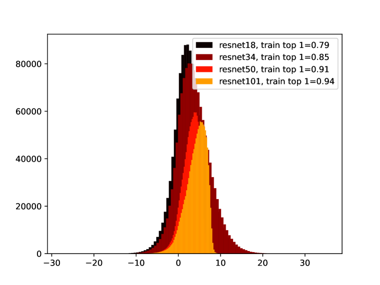
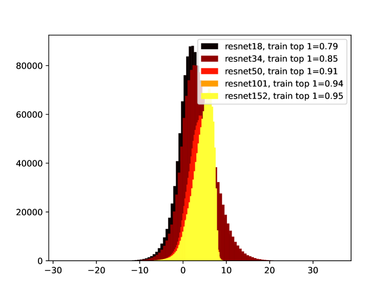
Figure 3: Distribution of the margins on the training set of ImageNet, with the pretrained ResNets available on PyTorch.

Details for sparse networks. ResNet18 is trained on $99\%$ of ImageNet with a single GPU using SGD for $90$ epochs, learning rate $0.1$, weight-decay $0.0001$, batch size $1024$, and a multi-step scheduler where the learning rate is divided by $10$ at epochs $30$, $60$ and $80$. The epoch out of the $90$ ones with maximum validation top 1 accuracy is considered as the final epoch. Pruning is done iteratively accordingly to (Frankle et al., 2021). We prune $20\%$ of the remaining weights of each convolutional layer, and $10\%$ of the final fully connected layer, at each pruning iteration, save the mask and rewind the weights to their values after the first $5$ epochs of the dense network, and train for $85$ remaining epochs, before pruning again etc. Results for a single run are shown in Figure 4.

Details for increasing the train size. Instead of training on $99\%$ of ImageNet ($n=1268355$), we trained a ResNet18 on $n/2^{k}$ samples drawn at random, for $1\leqslant k\leqslant 5$. For each given $k$, the results are averaged over 3 seeds. The hyperparameters are the same as for sparse networks (except that we do not perform any pruning here): 90 epochs etc. Results are in Figure 5.

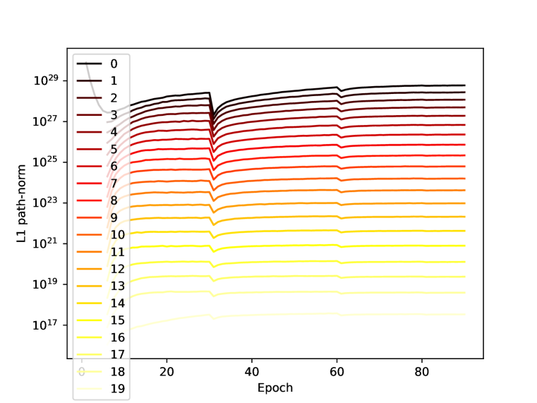
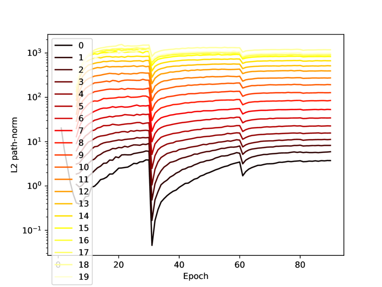
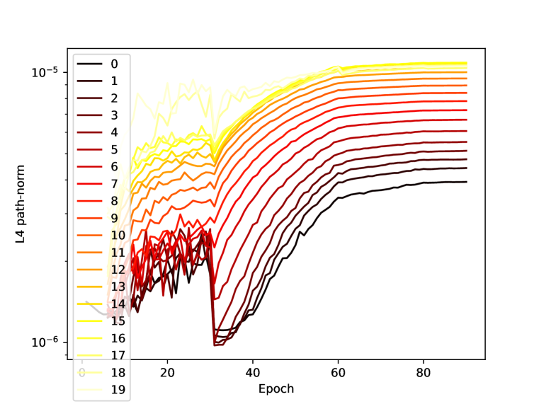
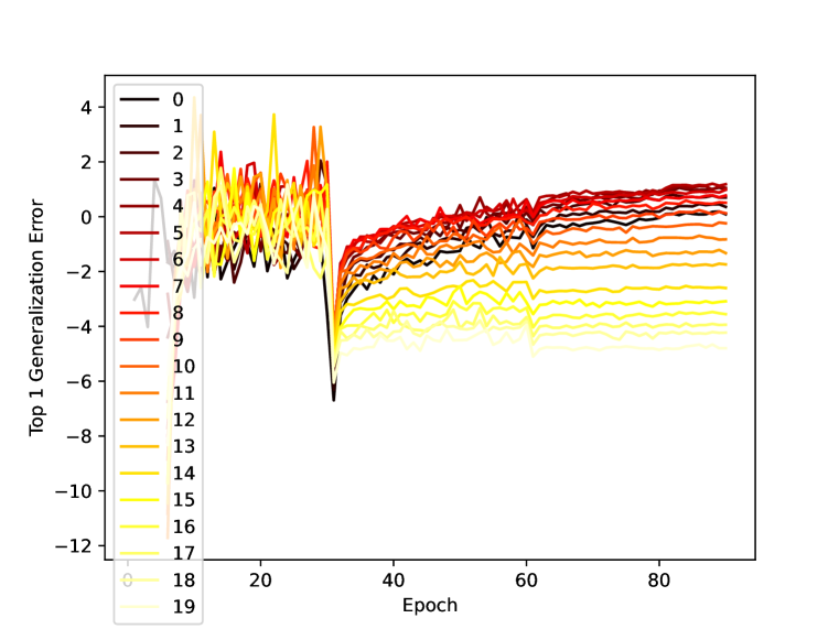
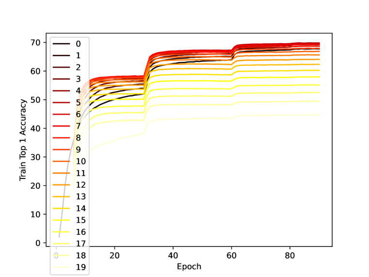
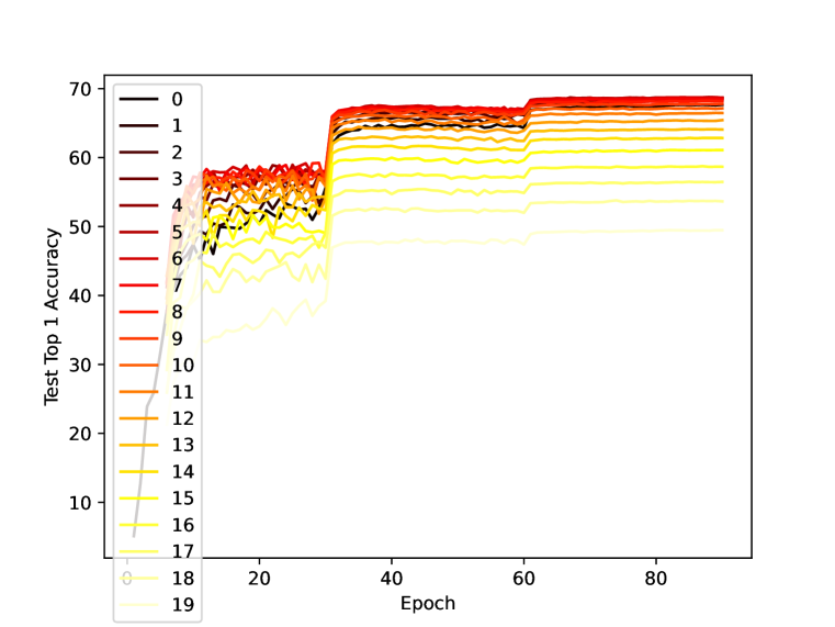
Figure 4: $L^{q}$ path-norm ($q=1,2,4$), test top 1 accuracy, training top 1 accuracy, and the top 1 generalization error (difference between test top 1 and train top 1) during the training of a ResNet18 on ImageNet. The pruning iteration is indicated in legend, with $0$ corresponding to the dense network. The color also indicates the degree of sparsity: from dense (black) to extremely sparse (yellow).

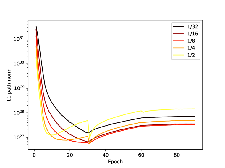
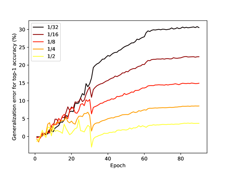
Figure 5: $L^{1}$ path-norm, and empirical generalization errors for both the top-1 accuracy and the cross-entropy during the training of a ResNet18 on a subset of the training images of ImageNet. The legend indicates the size of the subset considered, e.g. $1/m$ corresponds to $1/m$ of $99\%$ of ImageNet, leaving the other $1\%$ out for validation. The color also indicates the size of the subset: from small (black) to large (yellow).

Appendix J Main related works

Given the extent of the literature on generalization bounds, we apologize in advance for papers the reader may find missing below.

Previous definitions of the path-embedding and the path-activations In the work of (Kawaguchi et al., 2017, Section 5.1) the path-embedding and the path-activations are evoked in the case of a ReLU DAG with max-pooling neurons and no biases, but with no explicit definitions. Definition A.1 gives a formal definition for these objects, and extend it to the case where there are biases, which requires extending the path-embedding to paths starting from neurons that are not input neurons. Moreover, Definition A.1 extends it to arbitrary $k$-max-pooling neurons (classical max-pooling neurons correspond to $k=1$).

Note also that the formula Equation 1 is stated in the specific case of (Kawaguchi et al., 2017, Section 5.1) (as an explicit sum rather than an inner product), without proof since the objects are not explicitly defined in Kawaguchi et al. (2017).

A formal definition of the path-embedding is given in the specific case of ReLU feedforward neural networks with biases in the work of (Stock & Gribonval, 2022, Definition 6). Moreover, it is proved that Equation 1 holds in this specific case in (Stock & Gribonval, 2022, Corollary 3). Definition A.1 and Equation 1 generalize the latter to an arbitrary DAG with $*$-max-pooling or identity neurons (allowing in particular for skip connections, max-pooling and average-pooling).

The rest of the works we are aware of only define and consider the norm of the path-embedding, but not the embedding itself. The most general setting being the one of (Neyshabur et al., 2015) with a general DAG, but without max or identity neurons, nor biases. Not defining the path-embedding and the path-activations makes notations arguably heavier since Equation 1 is then always written with an explicit sum over all paths, with explicit product of weights along each path, and so on.

Previous generalization bounds based on path-norm See Table 1 for a comparison. Appendix K tackles some other bounds that do not appear in Table 1.

Empirical evaluation of path-norm The formula given in Theorem A.1 is the first one to fully encompass modern networks with biases, average/$*$-max-pooling, and skip connections, such as ResNets. An equivalent formula is stated for ReLU feedforward networks without biases (and no pooling/skip connections) in (Dziugaite et al., 2020, Appendix C.6.5) and (Jiang et al., 2020, Equations (43) and (44)) but without proof. Actually, this equivalent formula turns out to be false when there are $*$-max-pooling neurons as one must replace $*$-max-pooling neurons with identity ones, see Theorem A.1. Care must also be taken with average-pooling neurons that must be rescaled by considering them as identity neurons.

We could not find reported numerical values of the path-norm except for toy examples (Dziugaite, 2018; Furusho, 2020; Zheng et al., 2019). Details are in Appendix K.

Appendix K also discusses 1) inherent limitations of Theorem 3.1 which are common to many generalization bounds, and 2) the applicability of Theorem 3.1 compared to PAC-Bayes bounds.

Appendix K More Related Works

More generalization bounds using path-norm (E et al., 2022) establishes an additional bound to the one appearing in Table 1, for a class of functions and a complexity measure that are related to the infinite-depth limits of residual networks and the path-norm. However, it is unclear how this result implies anything for actual neural networks with the actual path-norm .

The bound in (Zheng et al., 2019) holds only for ReLU feedforward neural networks (no max or identity neurons) with no biases and it grows exponentially with the depth of the network. It is not included in Table 1 because it requires an additional assumption: the coordinates of the path-embedding must not only be bounded from above, but also from below. The reason for this assumption is not discussed in (Zheng et al., 2019), and it is unclear whether this is at all desirable, since a small path-norm can only be better for generalization in light of Theorem 3.1.

(Golowich et al., 2018, Theorem 4.3) is a bound that holds for ReLU feedforward neural networks with no biases (no max and no identity neurons) and it depends on the product of operators’ norms of the layers. It has the merit of having no dependence on the size of the architecture (depth, width, number of neurons etc.). However, it requires an additional assumption: each layer must have an operator norm bounded from below, so that it only applies to a restricted set of feedforward networks. Moreover, it is unclear whether such an assumption is desirable: there are networks with arbitrary small operators’ norms that realize the zero function, and the latter has a generalization error equal to zero.

Theorem 8 in (Kawaguchi et al., 2017) gives a generalization bound for scalar-valued (${d_{\textrm{out}}}=1$) models with an output of the form $\left\langle\Phi({\bm{\theta}}),{\bm{A}}({\bm{\theta}}^{\prime},x)x\right\rangle$ for some specific parameters ${\bm{\theta}},{\bm{\theta}}^{\prime}$ that have no reason to be equal. This is orthogonal to the case of neural networks where one must have ${\bm{\theta}}={\bm{\theta}}^{\prime}$, and it is therefore not included in Table 1. Theorem 5 in (Kawaguchi et al., 2017) can be seen as a possible first step to derive a bound based on path-norm in the specific case of the mean squared error loss. However, as discussed in more details below, (Kawaguchi et al., 2017, Theorem 5) is a rewriting of the generalization error with several terms that are as complex to bound as the original generalization error, resulting in a bound being as hard as the generalization error to evaluate/estimate.

More details about Theorem 5 in (Kawaguchi et al., 2017) We start by re-deriving Theorem 5 in (Kawaguchi et al., 2017). In the specific case of mean squared error, using that

$$\|R_{{\bm{\theta}}}(x)-y\|_{2}^{2}=\|R_{{\bm{\theta}}}(x)\|_{2}^{2}+\|y\|_{2}^{2}-2\left\langle R_{\bm{\theta}}(x),y\right\rangle,$$

it is possible to rewrite the generalization error as follows:

$$\textrm{generalization error of ${\hat{{\bm{\theta}}}}({\mathbf{Z}})$}= {\mathbb{E}}\left(\|R_{{\hat{{\bm{\theta}}}}({\mathbf{Z}})}(\tilde{{\mathbf{X}}})-\tilde{{\mathbf{Y}}}\|_{2}^{2}|{\mathbf{Z}}\right)-\frac{1}{n}\sum_{i=1}^{n}\|R_{{\hat{{\bm{\theta}}}}({\mathbf{Z}})}({\mathbf{X}}_{i})-{\mathbf{Y}}_{i}\|_{2}^{2}$$

$$= {\mathbb{E}}\left(\|R_{{\hat{{\bm{\theta}}}}({\mathbf{Z}})}(\tilde{{\mathbf{X}}})\|_{2}^{2}|{\mathbf{Z}}\right)-\frac{1}{n}\sum_{i=1}^{n}\|R_{{\hat{{\bm{\theta}}}}({\mathbf{Z}})}({\mathbf{X}}_{i})\|_{2}^{2}$$

$$+{\mathbb{E}}\left(\|\tilde{{\mathbf{Y}}}\|_{2}^{2}|{\mathbf{Z}}\right)-\sum_{i=1}^{n}\|{\mathbf{Y}}_{i}\|_{2}^{2}$$

$$-2{\mathbb{E}}\left(\left\langle R_{{\hat{{\bm{\theta}}}}({\mathbf{Z}})}(\tilde{{\mathbf{X}}}),\tilde{{\mathbf{Y}}}\right\rangle|{\mathbf{Z}}\right)-\frac{1}{n}\sum_{i=1}^{n}\left\langle R_{{\hat{{\bm{\theta}}}}({\mathbf{Z}})}({\mathbf{X}}_{i}),{\mathbf{Y}}_{i}\right\rangle.$$

It is then possible to make the $L^{2}$ path-norm appear. For instance, for one-dimensional output networks, it can be proven (see Lemma A.1) that $R_{\bm{\theta}}(x)=\left\langle\Phi({\bm{\theta}}),z(x,{\bm{\theta}})\right\rangle$ with $\Phi({\bm{\theta}})$ the path-embedding of parameters ${\bm{\theta}}$, and $z$ that typically depends on the path-activations and the input, so that the first term above can be rewritten

$$\Phi({\hat{{\bm{\theta}}}}({\mathbf{Z}}))^{T}\left({\mathbb{E}}\left(z(\tilde{{\mathbf{X}}},{\hat{{\bm{\theta}}}}({\mathbf{Z}}))z(\tilde{{\mathbf{X}}},{\hat{{\bm{\theta}}}}({\mathbf{Z}}))^{T}|{\mathbf{Z}}\right)-\frac{1}{n}\sum_{i=1}^{n}z({\mathbf{X}}_{i},{\hat{{\bm{\theta}}}}({\mathbf{Z}}))z({\mathbf{X}}_{i},{\hat{{\bm{\theta}}}}({\mathbf{Z}}))^{T}\right)\Phi({\hat{{\bm{\theta}}}}({\mathbf{Z}})).$$

Let us call a ”generalization error like quantity” any term of the form

$${\mathbb{E}}\left(f_{{\hat{{\bm{\theta}}}}({\mathbf{Z}})}(\tilde{{\mathbf{Z}}})|{\mathbf{Z}}\right)-\frac{1}{n}\sum_{i=1}^{n}f_{{\hat{{\bm{\theta}}}}({\mathbf{Z}})}({\mathbf{Z}}_{i}),$$

that is, any term that can be represented as a difference between the estimator learned from training data ${\mathbf{Z}}$ evaluated on test data $\tilde{{\mathbf{Z}}}$, and the evaluation on the training data. We see that the derivation above replaces the classical generalization error with two others quantities similar in definition to the generalization error. This derivation, which is specific to mean squared error, leads to Theorem 5 in (Kawaguchi et al., 2017). Very importantly, note that this derivation trades a single quantity similar to generalization error for two new such quantities. (Kawaguchi et al., 2017) does not discuss how to bound these two new terms, but without any further new idea, there is no other way than the ones developed in the literature so far: reduce the problem to bounding a Rademacher complexity (as it is done in Theorem 3.1), or use the PAC-Bayes framework, and so on.

More on numerical evaluation of path-norm (Dziugaite, 2018, Section 2.9.1) reports numerical evaluations after 5 epochs of SGD on a one hidden layer network trained on a binary variant of MNIST. (Furusho, 2020, Figure 9 and Section 3.3.1) deals with 1d regression with 5 layers and 100 width. (Zheng et al., 2019) experiments on MNIST. Note that it is not clear whether (Zheng et al., 2019) reports the path-norm as defined in Definition A.1. Indeed, (Zheng et al., 2019) quotes both (Neyshabur et al., 2015) and (Neyshabur et al., 2017) when refering to the path-norm, but these two papers have two different definitions of the path-norm, as (Neyshabur et al., 2017) normalize it by the margin while (Neyshabur et al., 2015) does not.

For completeness, let us also mention that (Dziugaite et al., 2020; Jiang et al., 2020) reports whether the path-norm correlates with the empirical generalization error or not, but do not report the numerical values. (Neyshabur et al., 2017) reports the path-norm normalized by the margins, but not separately from each other.

Inherent limitations of uniform convergence bounds Theorem 3.1 has some inherent limitations due to its nature. It is data-dependent as it depends on the input distribution. However, it does not depend on the label distribution, making it uninformative as soon as $\bm{\Theta}$ is so much expressive that it can fit random labels. Networks that can fit random labels have already been found empirically (Zhang et al., 2021), and it is open whether this stays true with a constraint on the path-norm.

Theorem 3.1 is based on a uniform convergence bound as any other bound also based on a control of a Rademacher complexity. (Nagarajan & Kolter, 2019) empirically argue that even the tightest uniform convergence bound holding with high probability must be loose on some synthetic datasets. If this was confirmed theoretically, this would still allow uniform bounds to be tight when considering other datasets than the one in (Nagarajan & Kolter, 2019), such as real-world datasets, or when the estimator considered in (Nagarajan & Kolter, 2019) is not in $\bm{\Theta}$ (for instance because of constraints on the slopes via the path-norm).

Finally, Theorem 3.1 can provide theoretical guarantees on the generalization error of the output of a learning algorithm, but only a posteriori, after training. In order to have a priori guarantees, one should have to derive a priori knowledge on the path-norm at the end of the learning algorithm.

Comparison to PAC-Bayes bounds Another interesting direction to understand generalization of neural networks is the PAC-Bayes framework (Guedj, 2019; Alquier, 2021). Unfortunately, PAC-Bayes bounds cannot be exactly computed on networks that are trained in a usual way. Indeed, these bounds typically involve a KL-divergence, or something related, for which there is no closed form except for very specific distributions (iid Gaussian/Cauchy weights…) that do not correspond to the distributions of the weights after a usual training. We are aware of two research directions that try to get over this issue. The first way is to change the learning algorithm by enforcing the weights to be iid normally distributed, and then optimize the parameters of these normal distributions, see for instance the pioneer work (Dziugaite & Roy, 2017). The merit of this new learning algorithm is that it has explicitly been designed with the goal of having a small generalization error. Practical performance are worse than with usual training, but this leads to networks with an associated non-vacuous generalization bound. To the best of our knowledge, this is the only way to get a non-vacuous bound

, and unfortunately, this does not apply to usual training. The second way to get over the intractable evaluation of the KL-divergence is to 1) try to approximate the bound within reasonable time, and 2) try to quantify the error made with the approximation (Pérez & Louis, 2020). Unfortunately, to the best of our knowledge, approximation is often based on a distribution assumption of the weights that is not met in practice (e.g. iid Gaussian weights), approximation is costly, and the error is unclear when applied to networks trained usually. For instance, the bound in (Pérez & Louis, 2020, Section 5) 1) requires at least $O(n^{2})$ operations to be evaluated, with $n$ being the number of training examples, thus being prohibitive for large $n$ (Pérez & Louis, 2020, Section 7), and 2) it is unclear what error is being made when using a Gaussian process as an approximation of the neural network learned by SGD.

References

- Alquier (2021) Pierre Alquier. User-friendly introduction to PAC-Bayes bounds. CoRR, abs/2110.11216, 2021. URL https://arxiv.org/abs/2110.11216.
- Anil et al. (2019) Cem Anil, James Lucas, and Roger B. Grosse. Sorting out Lipschitz function approximation. In Kamalika Chaudhuri and Ruslan Salakhutdinov (eds.), Proceedings of the 36th International Conference on Machine Learning, ICML 2019, 9-15 June 2019, Long Beach, California, USA, volume 97 of Proceedings of Machine Learning Research, pp. 291–301. PMLR, 2019. URL http://proceedings.mlr.press/v97/anil19a.html.
- Arora et al. (2017) Raman Arora, Amitabh Basu, Poorya Mianjy, and Anirbit Mukherjee. Understanding deep neural networks with rectified linear units. Electron. Colloquium Comput. Complex., 24:98, 2017. URL https://eccc.weizmann.ac.il/report/2017/098.
- (4) Francis Bach. Learning from first principles. URL https://www.di.ens.fr/~fbach/ltfp_book.pdf.
- Bach (2017) Francis R. Bach. Breaking the curse of dimensionality with convex neural networks. J. Mach. Learn. Res., 18:19:1–19:53, 2017. URL http://jmlr.org/papers/v18/14-546.html.
- Barron & Klusowski (2019) Andrew R. Barron and Jason M. Klusowski. Complexity, statistical risk, and metric entropy of deep nets using total path variation. CoRR, abs/1902.00800, 2019. URL http://arxiv.org/abs/1902.00800.
- Bartlett & Mendelson (2002) Peter L. Bartlett and Shahar Mendelson. Rademacher and Gaussian complexities: Risk bounds and structural results. J. Mach. Learn. Res., 3:463–482, 2002. URL http://jmlr.org/papers/v3/bartlett02a.html.
- Bartlett et al. (2017) Peter L. Bartlett, Dylan J. Foster, and Matus Telgarsky. Spectrally-normalized margin bounds for neural networks. In Isabelle Guyon, Ulrike von Luxburg, Samy Bengio, Hanna M. Wallach, Rob Fergus, S. V. N. Vishwanathan, and Roman Garnett (eds.), Advances in Neural Information Processing Systems 30: Annual Conference on Neural Information Processing Systems 2017, December 4-9, 2017, Long Beach, CA, USA, pp. 6240–6249, 2017. URL https://proceedings.neurips.cc/paper/2017/hash/b22b257ad0519d4500539da3c8bcf4dd-Abstract.html.
- Boucheron et al. (2013) Stéphane Boucheron, Gábor Lugosi, and Pascal Massart. Concentration inequalities. Oxford University Press, Oxford, 2013. ISBN 978-0-19-953525-5. doi: 10.1093/acprof:oso/9780199535255.001.0001. URL https://doi-org.acces.bibliotheque-diderot.fr/10.1093/acprof:oso/9780199535255.001.0001. A nonasymptotic theory of independence, With a foreword by Michel Ledoux.
- Dziugaite (2018) Gintare Karolina Dziugaite. Revisiting Generalization for Deep Learning: PAC-Bayes, Flat Minima, and Generative Models. PhD thesis, Department of Engineering University of Cambridge, 2018.
- Dziugaite & Roy (2017) Gintare Karolina Dziugaite and Daniel M. Roy. Computing nonvacuous generalization bounds for deep (stochastic) neural networks with many more parameters than training data. In Gal Elidan, Kristian Kersting, and Alexander Ihler (eds.), Proceedings of the Thirty-Third Conference on Uncertainty in Artificial Intelligence, UAI 2017, Sydney, Australia, August 11-15, 2017. AUAI Press, 2017. URL http://auai.org/uai2017/proceedings/papers/173.pdf.
- Dziugaite et al. (2020) Gintare Karolina Dziugaite, Alexandre Drouin, Brady Neal, Nitarshan Rajkumar, Ethan Caballero, Linbo Wang, Ioannis Mitliagkas, and Daniel M. Roy. In search of robust measures of generalization. In Hugo Larochelle, Marc’Aurelio Ranzato, Raia Hadsell, Maria-Florina Balcan, and Hsuan-Tien Lin (eds.), Advances in Neural Information Processing Systems 33: Annual Conference on Neural Information Processing Systems 2020, NeurIPS 2020, December 6-12, 2020, virtual, 2020. URL https://proceedings.neurips.cc/paper/2020/hash/86d7c8a08b4aaa1bc7c599473f5dddda-Abstract.html.
- E et al. (2022) Weinan E, Chao Ma, and Lei Wu. The Barron space and the flow-induced function spaces for neural network models. Constr. Approx., 55(1):369–406, 2022. ISSN 0176-4276. doi: 10.1007/s00365-021-09549-y. URL https://doi-org.acces.bibliotheque-diderot.fr/10.1007/s00365-021-09549-y.
- Frankle et al. (2020) Jonathan Frankle, David J. Schwab, and Ari S. Morcos. The early phase of neural network training. In 8th International Conference on Learning Representations, ICLR 2020, Addis Ababa, Ethiopia, April 26-30, 2020. OpenReview.net, 2020. URL https://openreview.net/forum?id=Hkl1iRNFwS.
- Frankle et al. (2021) Jonathan Frankle, Gintare Karolina Dziugaite, Daniel M. Roy, and Michael Carbin. Pruning neural networks at initialization: Why are we missing the mark? In 9th International Conference on Learning Representations, ICLR 2021, Virtual Event, Austria, May 3-7, 2021. OpenReview.net, 2021. URL https://openreview.net/forum?id=Ig-VyQc-MLK.
- Furusho (2020) Yasutaka Furusho. Analysis of Regularization and Optimization for Deep Learning. PhD thesis, Nara Institute of Science and Technology, 2020.
- Galanti et al. (2023) Tomer Galanti, Mengjia Xu, Liane Galanti, and Tomaso A. Poggio. Norm-based generalization bounds for compositionally sparse neural networks. CoRR, abs/2301.12033, 2023. doi: 10.48550/arXiv.2301.12033. URL https://doi.org/10.48550/arXiv.2301.12033.
- Golowich et al. (2018) Noah Golowich, Alexander Rakhlin, and Ohad Shamir. Size-independent sample complexity of neural networks. In Sébastien Bubeck, Vianney Perchet, and Philippe Rigollet (eds.), Conference On Learning Theory, COLT 2018, Stockholm, Sweden, 6-9 July 2018, volume 75 of Proceedings of Machine Learning Research, pp. 297–299. PMLR, 2018. URL http://proceedings.mlr.press/v75/golowich18a.html.
- Gonon et al. (2023) Antoine Gonon, Nicolas Brisebarre, Rémi Gribonval, and Elisa Riccietti. Approximation speed of quantized vs. unquantized ReLU neural networks and beyond. IEEE Transactions on Information Theory, 2023. doi: 10.1109/TIT.2023.3240360.
- Guedj (2019) Benjamin Guedj. A primer on PAC-Bayesian learning. CoRR, abs/1901.05353, 2019. URL http://arxiv.org/abs/1901.05353.
- He et al. (2016) Kaiming He, Xiangyu Zhang, Shaoqing Ren, and Jian Sun. Deep residual learning for image recognition. In 2016 IEEE Conference on Computer Vision and Pattern Recognition, CVPR 2016, Las Vegas, NV, USA, June 27-30, 2016, pp. 770–778. IEEE Computer Society, 2016. doi: 10.1109/CVPR.2016.90. URL https://doi.org/10.1109/CVPR.2016.90.
- Jiang et al. (2020) Yiding Jiang, Behnam Neyshabur, Hossein Mobahi, Dilip Krishnan, and Samy Bengio. Fantastic generalization measures and where to find them. In 8th International Conference on Learning Representations, ICLR 2020, Addis Ababa, Ethiopia, April 26-30, 2020. OpenReview.net, 2020. URL https://openreview.net/forum?id=SJgIPJBFvH.
- Kakade et al. (2008) Sham M. Kakade, Karthik Sridharan, and Ambuj Tewari. On the complexity of linear prediction: Risk bounds, margin bounds, and regularization. In Daphne Koller, Dale Schuurmans, Yoshua Bengio, and Léon Bottou (eds.), Advances in Neural Information Processing Systems 21, Proceedings of the Twenty-Second Annual Conference on Neural Information Processing Systems, Vancouver, British Columbia, Canada, December 8-11, 2008, pp. 793–800. Curran Associates, Inc., 2008. URL https://proceedings.neurips.cc/paper/2008/hash/5b69b9cb83065d403869739ae7f0995e-Abstract.html.
- Kawaguchi et al. (2017) Kenji Kawaguchi, Leslie Pack Kaelbling, and Yoshua Bengio. Generalization in deep learning. CoRR, abs/1710.05468, 2017. URL http://arxiv.org/abs/1710.05468.
- Ledoux & Talagrand (1991) Michel Ledoux and Michel Talagrand. Probability in Banach spaces, volume 23 of Ergebnisse der Mathematik und ihrer Grenzgebiete (3) [Results in Mathematics and Related Areas (3)]. Springer-Verlag, Berlin, 1991. ISBN 3-540-52013-9. doi: 10.1007/978-3-642-20212-4. URL https://doi.org/10.1007/978-3-642-20212-4. Isoperimetry and processes.
- Marcotte et al. (2023) Sibylle Marcotte, Rémi Gribonval, and Gabriel Peyré. Abide by the law and follow the flow: Conservation laws for gradient flows. CoRR, abs/2307.00144, 2023. doi: 10.48550/arXiv.2307.00144. URL https://doi.org/10.48550/arXiv.2307.00144.
- Maurer (2016) Andreas Maurer. A vector-contraction inequality for rademacher complexities. In Ronald Ortner, Hans Ulrich Simon, and Sandra Zilles (eds.), Algorithmic Learning Theory - 27th International Conference, ALT 2016, Bari, Italy, October 19-21, 2016, Proceedings, volume 9925 of Lecture Notes in Computer Science, pp. 3–17, 2016. doi: 10.1007/978-3-319-46379-7“˙1. URL https://doi.org/10.1007/978-3-319-46379-7_1.
- Nagarajan & Kolter (2019) Vaishnavh Nagarajan and J. Zico Kolter. Uniform convergence may be unable to explain generalization in deep learning. In Hanna M. Wallach, Hugo Larochelle, Alina Beygelzimer, Florence d’Alché-Buc, Emily B. Fox, and Roman Garnett (eds.), Advances in Neural Information Processing Systems 32: Annual Conference on Neural Information Processing Systems 2019, NeurIPS 2019, December 8-14, 2019, Vancouver, BC, Canada, pp. 11611–11622, 2019. URL https://proceedings.neurips.cc/paper/2019/hash/05e97c207235d63ceb1db43c60db7bbb-Abstract.html.
- Neyshabur (2017) Behnam Neyshabur. Implicit regularization in deep learning. CoRR, abs/1709.01953, 2017. URL http://arxiv.org/abs/1709.01953.
- Neyshabur et al. (2015) Behnam Neyshabur, Ryota Tomioka, and Nathan Srebro. Norm-based capacity control in neural networks. In Peter Grünwald, Elad Hazan, and Satyen Kale (eds.), Proceedings of The 28th Conference on Learning Theory, COLT 2015, Paris, France, July 3-6, 2015, volume 40 of JMLR Workshop and Conference Proceedings, pp. 1376–1401. JMLR.org, 2015. URL http://proceedings.mlr.press/v40/Neyshabur15.html.
- Neyshabur et al. (2017) Behnam Neyshabur, Srinadh Bhojanapalli, David McAllester, and Nati Srebro. Exploring generalization in deep learning. In Isabelle Guyon, Ulrike von Luxburg, Samy Bengio, Hanna M. Wallach, Rob Fergus, S. V. N. Vishwanathan, and Roman Garnett (eds.), Advances in Neural Information Processing Systems 30: Annual Conference on Neural Information Processing Systems 2017, December 4-9, 2017, Long Beach, CA, USA, pp. 5947–5956, 2017. URL https://proceedings.neurips.cc/paper/2017/hash/10ce03a1ed01077e3e289f3e53c72813-Abstract.html.
- Neyshabur et al. (2018) Behnam Neyshabur, Srinadh Bhojanapalli, and Nathan Srebro. A PAC-Bayesian approach to spectrally-normalized margin bounds for neural networks. In 6th International Conference on Learning Representations, ICLR 2018, Vancouver, BC, Canada, April 30 - May 3, 2018, Conference Track Proceedings. OpenReview.net, 2018. URL https://openreview.net/forum?id=Skz_WfbCZ.
- Pérez & Louis (2020) Guillermo Valle Pérez and Ard A. Louis. Generalization bounds for deep learning. CoRR, abs/2012.04115, 2020. URL https://arxiv.org/abs/2012.04115.
- Pitas et al. (2019) Konstantinos Pitas, Andreas Loukas, Mike Davies, and Pierre Vandergheynst. Some limitations of norm based generalization bounds in deep neural networks. CoRR, abs/1905.09677, 2019. URL http://arxiv.org/abs/1905.09677.
- Quemener & Corvellec (2013) E. Quemener and M. Corvellec. SIDUS—the Solution for Extreme Deduplication of an Operating System. Linux Journal, 2013.
- Shalev-Shwartz & Ben-David (2014) Shai Shalev-Shwartz and Shai Ben-David. Understanding Machine Learning - From Theory to Algorithms. Cambridge University Press, 2014. ISBN 978-1-10-705713-5. URL http://www.cambridge.org/de/academic/subjects/computer-science/pattern-recognition-and-machine-learning/understanding-machine-learning-theory-algorithms.
- Stock & Gribonval (2022) Pierre Stock and Rémi Gribonval. An embedding of ReLU networks and an analysis of their identifiability. Constructive Approximation, July 2022. ISSN 1432-0940. doi: 10.1007/s00365-022-09578-1. URL https://doi.org/10.1007/s00365-022-09578-1.
- von Luxburg & Bousquet (2004) Ulrike von Luxburg and Olivier Bousquet. Distance-based classification with Lipschitz functions. J. Mach. Learn. Res., 5:669–695, 2004. URL http://jmlr.org/papers/volume5/luxburg04b/luxburg04b.pdf.
- Wainwright (2019) Martin J. Wainwright. High-dimensional statistics, volume 48 of Cambridge Series in Statistical and Probabilistic Mathematics. Cambridge University Press, Cambridge, 2019. ISBN 978-1-108-49802-9. doi: 10.1017/9781108627771. URL https://doi-org.acces.bibliotheque-diderot.fr/10.1017/9781108627771. A non-asymptotic viewpoint.
- Zhang et al. (2021) Chiyuan Zhang, Samy Bengio, Moritz Hardt, Benjamin Recht, and Oriol Vinyals. Understanding deep learning (still) requires rethinking generalization. Commun. ACM, 64(3):107–115, 2021. doi: 10.1145/3446776. URL https://doi.org/10.1145/3446776.
- Zheng et al. (2019) Shuxin Zheng, Qi Meng, Huishuai Zhang, Wei Chen, Nenghai Yu, and Tie-Yan Liu. Capacity control of ReLU neural networks by basis-path norm. In The Thirty-Third AAAI Conference on Artificial Intelligence, AAAI 2019, The Thirty-First Innovative Applications of Artificial Intelligence Conference, IAAI 2019, The Ninth AAAI Symposium on Educational Advances in Artificial Intelligence, EAAI 2019, Honolulu, Hawaii, USA, January 27 - February 1, 2019, pp. 5925–5932. AAAI Press, 2019. doi: 10.1609/aaai.v33i01.33015925. URL https://doi.org/10.1609/aaai.v33i01.33015925.