Geodesic tracking of gravitational collapse and migration of boson stars

Abstract

Boson stars are potential sources of gravitational radiation. To improve our comprehension of these exotic objects, we present the study of geodesics within the space-times of stable, collapsing, and migrating boson stars. We focus on timelike geodesics that are initially circular or reciprocating. We verify that orbits initially bound within a stable boson stars persist in their bound states. For a collapsing boson star, we show that orbits initially bound and reciprocating finally either become unbound or plunge into the newly formed black hole, depending on their initial maximal radii. For initially circular geodesics, orbits with small radii plunge into the black hole; orbits with intermediate radii become unbound; and large radii orbits linger around the black hole with nonvanishing eccentricities. For the migrating case, a black hole does not form. In this case, the reciprocating orbits span a wider radial range. For initially circular geodesics, orbits with small radii become unbound, and orbits with large radii remain bound with nonvanishing eccentricities. This geodesic study provides a novel approach to investigate the gravitational collapse and migration of boson stars.

I Introduction

Since the first detection of gravitational waves from the coalescence of a binary black hole Abbott2016a , more than a hundred new gravitational-wave events have been observed by LIGO and VIRGO LIGOScientific:2018jsj ; LIGOScientific:2020kqk ; LIGOScientific:2021psn . These observations, together with the shadow observations of the black holes in M87*eth2019 and Sagittarius $A^{*}$eth2022 , are giving us an outstanding opportunity to gain a complete understanding of the nature of black holes, including the dynamics of their horizons.

The evidence from gravitational-wave detections strongly supports black holes and neutron stars as their sources and Einstein’s theory of general relativity as the correct theory of gravity. There is, however, still room for considering alternative theories of gravity and exotic compact objects that mimic black holes. Boson stars are well-known mimickers of black holes Feinblum1968 ; Kaup1968 ; Ruffini1969 ; Seidel1994 ; Giovanni2018 ; Sanchis2019 ; Cardoso:2019rvt . They have been recently considered Bustillo2021 as the objects behind the GW190521 event LIGOScientific:2020iuh . Thus, it is important to further improve our understanding of the properties of these exotic objects, and in particular, to determine the signatures that distinguish boson stars from black holes. Equally important is to identify situations in which gravitational-wave observations would be difficult to distinguish boson stars from black holes.

Nonlinear stability studies Sanchis-Gual:2019ljs ; Choptuik:2019zji ; Sanchis-Gual:2021edp ; Siemonsen:2020hcg ; Sanchis-Gual:2021phr point out that there are three types of boson stars: 1) unstable boson stars collapsing into black holes, 2) unstable boson stars that migrating to the stable configurations, and 3) stable boson stars. Thus, investigating the unstable branches of boson stars is important to gain further clues on scenarios leading to the formation of a black hole or a stable star.

Geodesics are a powerful tool to study static and fully dynamic space-times. They play a crucial role in understanding gravitational collapse and singularities via the incompleteness of the geodesic trajectories Penrose1965 ; Wald1984 . Null geodesics are also essential for identifying unexpected features in forming a common apparent horizon during the head-on collisions of black holes 1995Sci…270..941M . Null-geodesics can also be used to visualize the collision of binary black holes from numerical relativity simulations Vincent:2012kn ; Bohn:2014xxa .

Geodesics have been used to study boson stars under the equilibrium assumption, where novel orbits were identified philippe2014 ; Grould12017 ; Collodel2018 ; Yuzhang2021 ; Herdeiro2021lwl . It has also been shown how the properties of geodesics and light rings are tied to the stability of the boson stars Cunha:2017qtt ; multiplepr2022 ; multiplepr2022cai . By using nonlinear numerical evolutions of ultracompact boson stars under an adiabatic approximation, Cunha et al. Cunha:2022gde demonstrated that would trigger instabilities with two possible fates: migration to non-ultracompact configurations or collapse into black holes. They also showed that if a stable light ring finally disappears, the unstable boson star will migrate to a stable state or collapse into a black hole.

To gain further new insights, we would like to carry out fully nonlinear evolutions of boson stars and compute geodesics in the resulting dynamical space-time. The geodesic allows us to map the boson star space-time during its gravitational collapse and migration. We will focus on spherical boson stars and initially bounded time-like geodesics.

II Methodology

The action used for the boson star is Sanchis-Gual:2021phr

$$S=\int{d^{4}x\sqrt{-g}\left(\frac{R}{16\pi}-\frac{1}{2}\partial_{\mu}\Phi\partial^{\mu}\Phi^{*}-V(|\Phi|^{2})\right)},$$ (1)

where $\Phi$ is a complex scalar and the scalar potential is given by $V=\frac{1}{2}\mu^{2}|\Phi|^{2}+\frac{\lambda}{4}|\Phi|^{4}$. The units are such that $G=c=1$, and the mass parameter of the scalar field is set to $\mu=1$.

With an appropriate choice of the coupling parameter $\lambda$, one can construct initial configurations of boson stars that are stable, unstable collapsing into a black hole, and unstable migrating into a stable boson star Sanchis-Gual:2021phr .

We assume that the boson star is initially stationary, thus Sanchis-Gual:2021phr ,

$$\Phi=\phi(r)\exp\left(i\omega t\right)$$ (2)

and the metric is given by Sanchis-Gual:2021phr

$$ds^{2}=-e^{2f_{0}(r)}dt^{2}+e^{2f_{1}(r)}\left(dr^{2}+r^{2}\,d\Omega^{2}\right)$$ (3)

with $d\Omega^{2}=d\theta^{2}+\sin^{2}\theta d\varphi^{2}$. The field equations for this gravity system become ordinary differential equations for the radial functions $f_{0}(r)$ and $f_{1}(r)$, together with an equation for $\phi(r)$. The only input needed to construct the initial boson star configuration is the parameters $\lambda$ and $\omega$.

We consider three types of boson stars: i) a stable boson star, ii) an unstable boson star that collapses into a black hole, and iii) an unstable boson star that migrates into another boson star. The parameters $\lambda$ and $\omega$ for each configuration are provided in Table 1. The Arnowitt-Deser-Misner mass $M$ for each boson star and the mass $M_{h}$ of the black hole for the collapsing cases are also included in Table 1. The corresponding profiles for $\phi(r)$ are depicted in Fig. 1.

Table 1: The coupling parameter $\lambda$, frequency $\omega$, ADM mass $M$, outcome, and mass $M_{h}$ for the unstable collapsing boson stars. All quantities are given in units of $M_{0}=\mu^{-1}$.

Case	$\lambda\,M_{0}^{2}/(4\pi)$	$\omega\,M_{0}$	$M/M_{0}$	Outcome	$M_{\text{h}}/M_{0}$
BS_a	100	0.92	2.194	stable	—
BS_b	0	0.88	1.357	collapse	1.246
BS_c	0	0.92	1.284	collapse	1.254
BS_d	50	0.96	1.828	migration	—

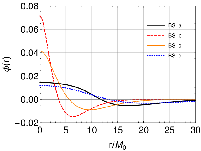
Figure 1: Initial profiles of the scalar field $\phi(r)$ for the models listed in Table 1.

Given the initial data for each boson star, the space-time evolution is carried out with our spherical numerical relativity code. The code solves the Baumgarte–Shapiro–Shibata–Nakamura formalism in spherical coordinates Montero:2012yr in terms of the following metric

$$ds^{2}=-\alpha^{2}dt^{2}+\gamma_{ij}(dx^{i}+\beta^{i}dt)(dx^{j}+\beta^{j}dt)$$ (4)

with $\beta^{i}=(\beta^{r},0,0)$ and the spacial line element

$$dl^{2}=e^{4\chi}\left(a(t,r)dr^{2}+r^{2}b(t,r)(d\theta^{2}+\sin^{2}\theta d\varphi^{2})\right).$$ (5)

For gauge conditions, we use the non-advective $1+\log$ for the lapse function $\alpha$ Bona:1997hp , and a variation of the gamma-driver condition for the shift vector $\beta^{r}$ Alcubierre:2002kk . We impose radiative boundary conditions Alcubierre:2002kk to reduce the unphysical reflections at the outer boundary. We adopt the fourth-order Kreiss-Oliger dissipation Kreiss-Oliger for stability. Temporal updating is done via method-of-lines with a second-order partially implicit Runge-Kutta method Montero:2012yr . The computational grid extends into a radius of $2,000M_{0}$, with a grid-spacing $\delta r=0.05M_{0}$. We use a time-step $\delta t=0.002M_{0}$. Since this work focuses on geodesics, we only show in Fig. 2 the evolution of the lapse function for each of the models listed in Table 1. The lapse function remains constant for the stable case, BS_a. As expected, the lapse function collapses for cases BS_b and BS_c, signaling the formation of a black hole. The oscillatory behavior is for the migrating case BS_d, where the boson star transforms into the stable configuration.

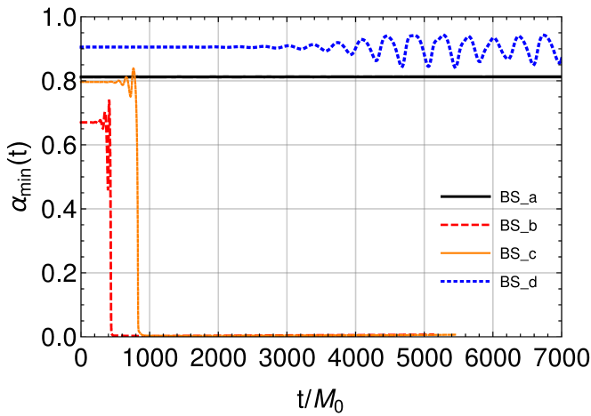
Figure 2: Evolution of minimum value of the lapse function $\alpha_{\text{min}}$ for the models listed in Table 1.

Geodesic integration is calculated in situ. That is, the geodesic equations are integrated in parallel with the space-time integration by interpolating the metric from the numerical grid to the geodesic Vincent:2012kn ; Bohn:2014xxa . A fourth-order Runge-Kutta temporal integration is used to solve the geodesic equations. Regarding the initial conditions of the geodesics, for simplicity, we only consider time-like geodesics initially bounded and in the equatorial plane. Two types of initial conditions are investigated: initially circular orbits and radial (reciprocating) orbits. Although the unstable boson star will either collapse into a black hole or migrate to other state, it is initially, to a good approximation, stationary and possesses a timelike killing vector $\xi^{\mu}=(\partial_{t})^{\mu}$ and a spacelike killing vector $\eta^{\mu}=(\partial_{\varphi})^{\mu}$. Thus we can set the initial data of the geodesics in terms of the initial energy $E/m=-(\partial_{t})^{\mu}u_{\mu}$, the angular momentum $J/m^{2}=(\partial_{\varphi})^{\mu}u_{\mu}$ ($m$ is the mass of the test particle), and the radial effective potentials based on the decomposition of the radial velocity Grould12017 ; Collodel2018 ; Yuzhang2021 . Because we are only considering initially circular and reciprocating orbits, the initial conditions of orbits are fully characterized by their initial radii.

III Results

We will first discuss the results for the case of initially bounded geodesics in the stable space-time of BS_a. We consider geodesics with three different maximal radii $r/M_{0}=\{3,9,15\}$ for both of the reciprocating and circular orbits. Figure 3 shows the radial distance of the orbit as a function of time. Solid lines are for the reciprocating orbits and dash lines for circular orbits. Since the boson star is stable, i.e., the space-time is not dynamical, the orbits remain reciprocating with the same maximum and minimum radial distance and circular with the constant radius. That is, the initially bounded geodesic orbits remain unchanged.

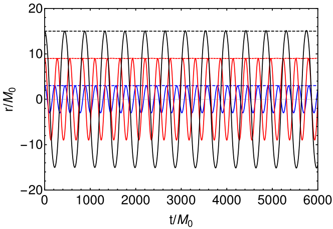
Figure 3: Evolution of the radial distance for circular and reciprocating geodesics in the space-time of case BS_a. Dashed and solid lines are for the circular and reciprocating orbits, respectively.

Next, we focus on the unstable boson stars: boson stars collapsing into black holes or migrating into other states. For unstable collapsing boson stars, we consider the cases BS_b and BS_c, with the latter has a longer lifetime than the former. As mentioned before, the orbits are initially bounded. There are only three outcomes: i) the orbit becomes unbound from the final black hole; ii) the orbit plunges into the black hole; iii) the orbit remains in a stable path around the black hole. To be able to get a reasonable map of the space-time, we consider a family of geodesics, for both the circular and reciprocating cases, with initial radii in the range $r/M_{0}\in[3,21]$ at intervals of $\Delta r/M_{0}=0.1$.

The evolution of an unstable boson star collapsing into a black hole has three phases. The first is a quasi-equilibrium phase in which the space-time remains almost unchanged. In the second phase, the boson star oscillates and eventually collapses into a black hole. During the third phase, the black hole grows from accreating the remnant scalar field. Figures 4 and 5 show the evolution of the radial coordinate of the geodesics for the cases BS_b and BS_c, respectively. The shaded regions are plotted as light blue for the quasi-equilibrium phase, light orange for the oscillating and collapsing phase, and light green for the black hole accretion growth phase. Blue lines denote geodesics that become unbound; red lines are geodesics that plunge into the black hole; and orange lines are for orbits that remain bounded but do not plunge. Panel (a) is for initially reciprocating orbits, and panel (b) is for initially circular orbits.

As seen in panel (a) of Figs. 4 and 5, reciprocating orbits remain reciprocating, that is, oscillating back and forth through the origin, during the quasi-equilibrium and collapsing phases. Once the black hole forms, some orbits plunge, and others become unbound depending on the corresponding initial maximal radii. For initial radius $r/M_{0}<14.7$ for BS_b and $r/M_{0}<15.6$ for BS_c, the geodesics plunge once the black hole forms. For radii $14.7\leq r/M_{0}\leq 15.4$ for BS_b and $15.6\leq r/M_{0}\leq 16.1$ for BS_c, the orbits become unbound. Orbits with initial radius $r/M_{0}>15.4$ for BS_b and $r/M_{0}>16.1$ for BS_c also plunge. Whether an orbit plunges or not depends on the radial distance the orbit has at the moment the black hole forms. The formation of the black hole changes the effective potential; thus, the radial position of the geodesic relative to the new location of the potential barrier determines the fate of the orbit, i.e., plunge or unbound.

For orbits initially circular, we observe from panel (b) in Figs. 4 and 5 that they remain circular during the quasi-equilibrium and collapsing phases. When they enter the black hole growth phase, the orbits will plunge if the initial radius satisfies $r/M_{0}<7.9$ for BS_b and $r/M_{0}<11.2$ for BS_c. If the initial radius satisfies $r/M_{0}>8.6$ for BS_b and $r/M_{0}>11.9$ for BS_c, the orbits will remain bound but become eccentric. And finally, if the initial radius belongs to $7.9\leq r/M_{0}\leq 8.6$ for BS_b and $11.2\leq r/M_{0}\leq 11.9$ for BS_c, the orbits will become unbound. The outcomes here have similar reasons to the reciprocating case, namely the location of the potential barrier and height relative to the position of the geodesic at the time of black hole formation.

In summary, the qualitative behaviors of the orbits for BS_b and BS_c are similar. The specific differences are due to the duration of the phases in each case.

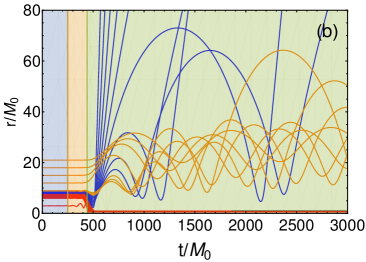
Figure 4: Evolution of the radial distance for the case BS_b. The shaded regions are plotted in light blue for the quasi-equilibrium phase, in light orange for the oscillating and collapsing phase, and in light green for the black hole accretion growth phase. Blue lines denote geodesics that become unbound; red lines are geodesics that plunge into the black hole; and orange lines are for orbits that remain bounded but do not plunge. Panel (a) is for initially reciprocating orbits, and panel (b) is for initially circular orbits.

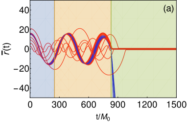
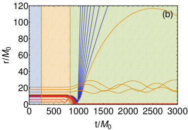
Figure 5: Same as Fig. 4 but for the BS_c case.

Finally, we discuss the results for the unstable migrating case BS_d, where the boson star migrates to a new equilibrium state and a black hole does not form. Figure 6 shows the evolution of the geodesic radial distance for this case. In this situation there are two distinct boson star evolution phases. As the previous case, the first phase is also the quasi-equilibrium phase with the space-time almost unchanged. The second phase is the proper oscillating and migrating phase, with the space-time changing until it settles down into a new equilibrium state. For all the reciprocating geodesic orbits, we do not observe a critical radius separating bound orbits from unbound ones. As seen in panel (a) of Fig. 6, bound and unbound orbits occur at both small and large radii. For all the initial stable circular orbits, we observe similar behaviors to that of the reciprocating orbits. Those that remain bound will have nozero eccentricities at late time. Such behaviors are completely different from the collapsing case.

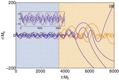
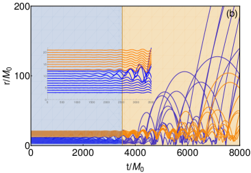
Figure 6: Same as Fig. 4 but for the BS_d case. Here the light blue background region is the quasi-equilibrium phase, the light orange background region is the oscillating and migrating phase.

IV Conclusions

We have presented results from a study of the behavior of geodesics in the dynamical space-times of boson stars. The geodesic integration was carried out simultaneously with the numerical evolution of the space-times. The work focused on initially bound orbits. In the stable boson star case, we verified that the state of the orbits remain unchanged. In the two unstable boson stars that collapse into black holes, we found that initially reciprocating and initially circular orbits have similar general fate. Orbits with small and large initial radii plunge into the black hole, and orbits with intermediate radii escape from the black hole. For the migrating boson star, there was no clear pattern, and orbits escape or remain bound but become eccentric.

The study has given us a picture of the gravitational collapse and migration of boson stars in terms of the dynamics of geodesics. As expected, the change of the space-time of the boson stars reflects on the change of the effective potential that governs the dynamics of the geodesics. The regions with separating, bound, unbound, and plunge orbits could potentially offer new insights into the behavior of matter in the vicinity of these objects, which could, in turn, be reflected in the emitted gravitational waves.

V Acknowledgments

We warmly thank Pedro V. P. Cunha for useful discussions and suggestions. This work was supported in part by the National Key Research and Development Program of China (Grant No. 2020YFC2201503), the National Natural Science Foundation of China (Grants No. 12105126, No. 11875151, No. 12075103, and No 12247101), the 111 Project under (Grant No. B20063), the China Postdoctoral Science Foundation (Grant No. 2021M701531), the Major Science and Technology Projects of Gansu Province, and “Lanzhou City’s scientific research funding subsidy to Lanzhou University”. P.L. was supported by NSF awards 2207780, 2114581, and 2114582.

References

- (1) B. P. Abbott et al. [LIGO Scientific Collaboration and Virgo Collaboration], Phys. Rev. Lett. 116, 061102 (2016).
- (2) B. P. Abbott et al. [LIGO Scientific Collaboration and Virgo Collaboration], Astrophys. J. Lett. 882, L24 (2019).
- (3) R. Abbott et al. [LIGO Scientific Collaboration and Virgo Collaboration], Astrophys. J. Lett. 913, L7 (2021).
- (4) R. Abbott et al. [LIGO Scientific, VIRGO and KAGRA], [arXiv:2111.03634 [astro-ph.HE]].
- (5) K. Akiyama et al. [Event Horizon Telescope], Astrophys. J. Lett. 875, L1 (2019); Astrophys. J. Lett. 875, L2 (2019); Astrophys. J. Lett. 875, L3 (2019); Astrophys. J. Lett. 875, L4 (2019); Astrophys. J. Lett. 875, L5 (2019); Astrophys. J. Lett. 875, L6 (2019).
- (6) K. Akiyama et al. [Event Horizon Telescope], Astrophys. J. Lett. 930, L12 (2022); Astrophys. J. Lett. 930, L13 (2022); Astrophys. J. Lett. 930, L14 (2022); Astrophys. J. Lett. 930, L15 (2022); Astrophys. J. Lett. 930, L16 (2022); Astrophys. J. Lett. 930, L17 (2022).
- (7) D. A. Feinblum and W. A. McKinley, Phys. Rev. 168, 1445 (1968).
- (8) D. J. Kaup, Phys. Rev. 172, 1331 (1968).
- (9) R. Ruffini and S. Bonazzola, Phys. Rev. 187, 1767 (1969).
- (10) E. Seidel and W.-M. Suen, Phys. Rev. Lett. 72, 2516 (1994).
- (11) F. D. Giovanni, N. Sanchis-Gual, C. A. R. Herdeiro, and J. A. Font, Phys. Rev. D 98, 064044 (2018).
- (12) N. Sanchis-Gual, F. D. Giovanni, M. Zilhão, C. A. R. Herdeiro, P. Cerda-Duran, J. A. Font, and E. Radu, Phys. Rev. Lett. 123, 221101 (2019).
- (13) V. Cardoso and P. Pani, Living Rev. Rel. 22, 4 (2019).
- (14) J. C. Bustillo, N. Sanchis-Gual, A. Torres-Forné, J. A. Font, A. Vajpeyi, R. Smith, C. A. R. Herdeiro, E. Radu, and S. H. W. Leong, Phys. Rev. Lett. 126, 081101 (2021).
- (15) R. Abbott et al. [LIGO Scientific Collaboration and Virgo Collaboration], Phys. Rev. Lett. 125, 101102 (2020).
- (16) N. Sanchis-Gual, F. D. Giovanni, M. Zilhão, C. A. R. Herdeiro, P. Cerdá-Durán, J. A. Font, and E. Radu, Phys. Rev. Lett. 123, 221101 (2019).
- (17) N. Siemonsen and W. E. East, Phys. Rev. D 103, 044022 (2021).
- (18) M. Choptuik, R. Masachs, and B. Way, Phys. Rev. Lett. 123, 131101 (2019).
- (19) N. Sanchis-Gual, F. D. Giovanni, C. A. R. Herdeiro, E. Radu, and J. A. Font, Phys. Rev. Lett. 126, 241105 (2021).
- (20) N. Sanchis-Gual, C. A. R. Herdeiro, and E. Radu, Class. Quant. Grav. 39, 064001 (2022).
- (21) R. Penrose, Phys. Rev. Lett. 14, 57 (1965).
- (22) R. M. Wald, “General Relativity”, The University of Chicago Press (1984).
- (23) R. A. Matzner, H. E. Seidel, S. L. Shapiro, L. Smarr, W. M. Suen, S. A. Teukolsky, and J. Winicour, Science 270, 941 (1995).
- (24) F. H. Vincent, E. Gourgoulhon, and J. Novak, Class. Quant. Grav. 29, 245005 (2012).
- (25) A. Bohn, W. Throwe, F. Hébert, K. Henriksson, D. Bunandar, M. A. Scheel, and N. W. Taylor, Class. Quant. Grav. 32, 065002 (2015).
- (26) C. A. R. Herdeiro, A. M. Pombo, E. Radu, P. V. P. Cunha, and N. Sanchis-Gual, JCAP 04, 051 (2021).
- (27) P. Grandclément, Claire Somé, and Eric Gourgoulhon, Phys. Rev. D, 90, 024068, (2014).
- (28) M. Grould, Z. Meliani, F. H. Vincent, P. Grandclément, and E. Gourgoulhon, Class. Quan. Grav. 34, 215007 (2017).
- (29) L. G. Collodel, B. Kleihaus, and J. A. Kunz, Phys. Rev. Lett. 120, 201103 (2018).
- (30) Y.-P. Zhang, Y.-B. Zeng, Y.-Q. Wang, S.-W. Wei, and Y.-X. Liu, Phys. Rev. D 105, 044021 (2022).
- (31) P. V. P. Cunha, E. Berti, and C. A. R. Herdeiro, Phys. Rev. Lett. 119, 251102 (2017).
- (32) Y.-Q. Chen, G.-Z. Guo, P. Wang, H.-W. Wu, and H.-T. Yang, Sci. China-Phys. Mech. Astron. 65, 120412 (2022).
- (33) Y.-F. Cai, Sci. China-Phys. Mech. Astron. 65, 120431 (2022).
- (34) P. V. P. Cunha, C. A. R. Herdeiro, E. Radu, and N. Sanchis-Gual, Phys. Rev. Lett. 130, 061401 (2023).
- (35) P. J. Montero and I. Cordero-Carrion, Phys. Rev. D 85, 124037 (2012).
- (36) C. Bona, J. Masso, E. Seidel, and J. Stela, Phys. Rev. D 56, 3405 (1997).
- (37) M. Alcubierre, B. Bruegmann, P. Diener, M. Koppitz, D. Pollney, E. Seidel, and R. Takahashi, Phys. Rev. D 67, 084023 (2003).
- (38) H.-O. Kreiss and J. Oliger, Methods for the Approximate Solution of the Time Dependent Problems (GARP, Geneva, 1973).