Escaping of Fast Radio Bursts

Abstract

We reconsider the escape of high brightness coherent emission of Fast Radio Bursts (FRBs) from magnetars’ magnetospheres, and conclude that there are numerous ways for the powerful FRB pulse to avoid nonlinear absorption. Sufficiently strong surface magnetic fields, $\geq 10\%$ of the quantum field, limit the waves’ non-linearity to moderate values. For weaker fields, the electric field experienced by a particle is limited by a combined ponderomotive and parallel-adiabatic forward acceleration of charges by the incoming FRB pulse along the magnetic field lines newly opened during FRB/Coronal Mass Ejection (CME). As a result, particles surf the weaker front part of the pulse, experiencing low radiative losses, and are cleared from the magnetosphere for the bulk of the pulse to propagate. We also find: (i) for propagation across magnetic field, the O-mode suffers much smaller dissipation than the X-mode; (ii) quasi-parallel propagation suffers minimal dissipation; (iii) initial mildly relativistic radial plasma flow further reduces losses; (iv) for oblique propagation of a pulse with limited transverse size, the leading part of the pulse would ponderomotively sweep the plasma aside.

1 Introduction

Observations of correlated radio and X-ray bursts (CHIME/FRB Collaboration et al., 2020; Ridnaia et al., 2021; Bochenek et al., 2020; Mereghetti et al., 2020; Li et al., 2021) established the FRB-magnetar connection. There is a long list of arguments in favor of magnetospheric loci of FRBs (e.g.  Lyutikov, 2003; Popov & Postnov, 2013; Lyutikov et al., 2016; Lyutikov & Popov, 2020), as opposed, e.g.  to the wind (e.g.  Lyubarsky, 2014; Beloborodov, 2017; Metzger et al., 2019; Thompson, 2022) (see also reconsideration of wind dynamics by Sharma et al. (2023), arguing against appearance of shocks). For example, temporal coincidence between the radio and X-ray profiles, down to milliseconds is a strong argument in favor of magnetospheric origin (Lyutikov & Popov, 2020): we know that X-ray are magnetospheric events, as demonstrated by the periodic oscillations seen in giant flares (Palmer et al., 2005; Hurley et al., 2005).

In fact, strong magnetic fields  are needed in the emission region to suppress strong ‘normal” (non-coherent) loses in magnetar magnetospheres. In the absence of strong guide-field a coherently emitting particle will lose energy on time scales shorter than the coherent low frequency wave. Lyutikov et al. (2016); Lyutikov & Rafat (2019). It is required that the cyclotron frequency be much larger than the wave frequency in the emission region. This requirement limits emission regions to the magnetospheres  of neutron stars.

A somewhat separate issue is the escape of the powerful radio waves from the magnetosphere: as the waves propagate in the (presumably) dipole magnetosphere  their amplitude decrease slower than that of the guide field. Beloborodov (2021, 2022, 2023) argued that strong electromagnetic wave, even if generated with the magnetars’ magnetospheres, would not escape. The argument, in the simplest form, goes as: when the electromagnetic field becomes larger than the guide field, for some waves, for which there is a component of the wave’s magnetic field along the guide field, there are periodic instances when electric field becomes larger than the magnetic field. This lead to efficient particle acceleration, and dissipation of the wave’s energy. Along similar line of reasoning, Golbraikh & Lyubarsky (2023) argued that the nonlinear decay of the fast magnetosonic into the Alfvén   waves would lead to efficient energy dissipation of the wave.

Here we argue that the particular case considered in Beloborodov (2021, 2022, 2023) are extreme, not indicative of the more general situation (see also Qu et al., 2022). Most importantly, ponderomotive acceleration results in a very slow rate of overtaking the particle by the wave - particles surf the weaker rump-up part of the pulse for a long time, experiencing mild local intensity of the wave, and radiative losses much smaller than in the fully developed pulse. Same criticism applies to Golbraikh & Lyubarsky (2023) - ponderomotive acceleration would greatly reduce the efficiency of non-linear waves’ interaction (by approximately $\sim\gamma_{\parallel}^{3}\gg 1$).

Several other related issues are: (i) geometry of the magnetic field and wave polarization: Beloborodov (2021, 2022, 2023) considered X-mode (when the magnetic field of the wave adds/subtracts from the guide field) propagating nearly perpendicularly with respect to the guide field (e.g. , strictly equatorial propagation considered in Beloborodov, 2023) - this is the most dissipative case.

2 Non-linear electromagnetic waves with guide field

2.1 Basic parameters

There are several important parameters for non-linear wave-particle interaction. First there is the laser non-linearity parameter (Akhiezer et al., 1975)

$$a_{0}\equiv\frac{eE_{w}}{m_{e}c\omega}$$ (1)

where $E_{w}=B_{w}$ is the electric field in the coherent wave, and $\omega$ is the frequency (parameter $a_{0}$ is Lorentz invariant). In the absence of guide field the nonlinearity parameter (1) is of the order of a dimensionless momentum of transverse motion of a particle in the EM wave, in the frame where particle is on average at rest. In this case (no guide field), for $a_{0}\geq 1$ the particle motion becomes relativistic. The transverse Lorentz factor, as measured in the gyration frame is $\gamma_{0}=\sqrt{1+a_{0}^{2}}$ (for circularly polarized waves; $\gamma_{0}=\sqrt{1+a_{0}^{2}/2}$ for linearly polarized wave).

The second important parameter is the relative amplitude of the electromagnetic field of the wave with respect to the guide field

$$\delta=\frac{B_{w}}{B_{0}}$$ (2)

Then, there is the ratio of the cyclotron frequency to wave frequency

$$f=\frac{\omega_{B}}{\omega}$$ (3)

The three parameters combine

$$a_{0}=\delta f$$ (4)

The corresponding combination on the rhs is Lorentz invariant under a boost along the guide magnetic field.

It turns out, see Eq. (30), that another important combination is

$$\tilde{a}_{0}=\frac{a_{0}}{1+f}$$ (5)

This is effective non-linearity parameter for non-linear electromagnetic wave in finite guide field (parameter $f$ is defined in the lab frame, where initially a particle is at rest.).

2.2 FRBs’ parameters

For fiducial estimates, consider an FRB pulse coming from $d$= Gpc, of duration $\tau=1$ msec, and producing flux $F_{\nu}$ = 1 Jy at frequency of $\nu=10^{9}$ Hz (these values are at the higher end of the FRB parameters). The isotropic equivalent luminosity and total energy (in radio) are then

$$L_{iso}=4\pi D^{2}\nu F_{\nu}=10^{42}{\rm erg\,s}^{-1}\mbox{}$$

$$E_{iso}=L_{iso}\tau=10^{39}{\rm erg}$$ (6)

The electromagnetic field of the wave at distance $r$ from the source is

$$B_{w}=\frac{2\sqrt{\pi}\sqrt{\nu F_{\nu}}d}{\sqrt{c}r}=6\times 10^{9}\left(\frac{r}{R_{NS}}\right)^{-1}\,{\rm G}$$ (7)

The laser non-linearity parameter then evaluates to

$$a_{0}^{\ast}=\frac{e\sqrt{F_{\nu}}d}{\sqrt{\pi}m_{e}c^{3/2}\nu^{1/2}R_{NS}}=10^{7}$$ (8)

If we normalize the surface magnetic field to the quantum field

$$B_{NS}=b_{q}B_{Q}\mbox{}$$

$$B_{Q}=\frac{c^{3}m_{e}^{2}}{e\hbar}$$ (9)

and for now assume dipolar field

$$B_{0}=B_{NS}(r/R_{NS})^{-3}\mbox{}$$

$$a_{0}=a_{0}^{\ast}(r/R_{NS})^{-1},$$ (10)

then the relative amplitude of the fluctuating field and the ratio of frequencies are

$$\delta=\frac{B_{w}}{B_{0}}=\frac{2\sqrt{\pi}d\sqrt{\nu F_{\nu}}r^{2}}{\sqrt{c}B_{NS}R_{NS}}=10^{-4}b_{q}^{-1}\left(\frac{r}{R_{NS}}\right)^{2}\mbox{}$$

$$f=b_{q}\frac{eB_{Q}}{2\pi m_{e}c\nu}\left(\frac{r}{R_{NS}}\right)^{-3}=10^{11}b_{q}\left(\frac{r}{R_{NS}}\right)^{-3}$$ (11)

see Figs. 1.

The amplitude of electromagnetic fluctuations in the wave becomes comparable to the guide field ($\delta\sim 1$) at

$$\frac{r_{0}}{R_{NS}}\approx 10^{2}b_{q}^{1/2}$$ (12)

At that point

$$a_{0}[r_{0}]\approx 2\times 10^{5}\mbox{}$$

$$f(r_{0})=a_{0}[r_{0}]=2\times 10^{5}$$ (13)

The wave’s frequency equals cyclotron frequency at

$$\frac{r_{f}}{r_{0}}=a_{0}[r_{0}]^{1/3}\mbox{}$$

$$\frac{r_{f}}{R_{NS}}\approx 5\times 10^{3}b_{q}^{1/3}\mbox{}$$

$$a_{0}(r_{f})=a_{0}[r_{0}]^{2/3}$$ (14)

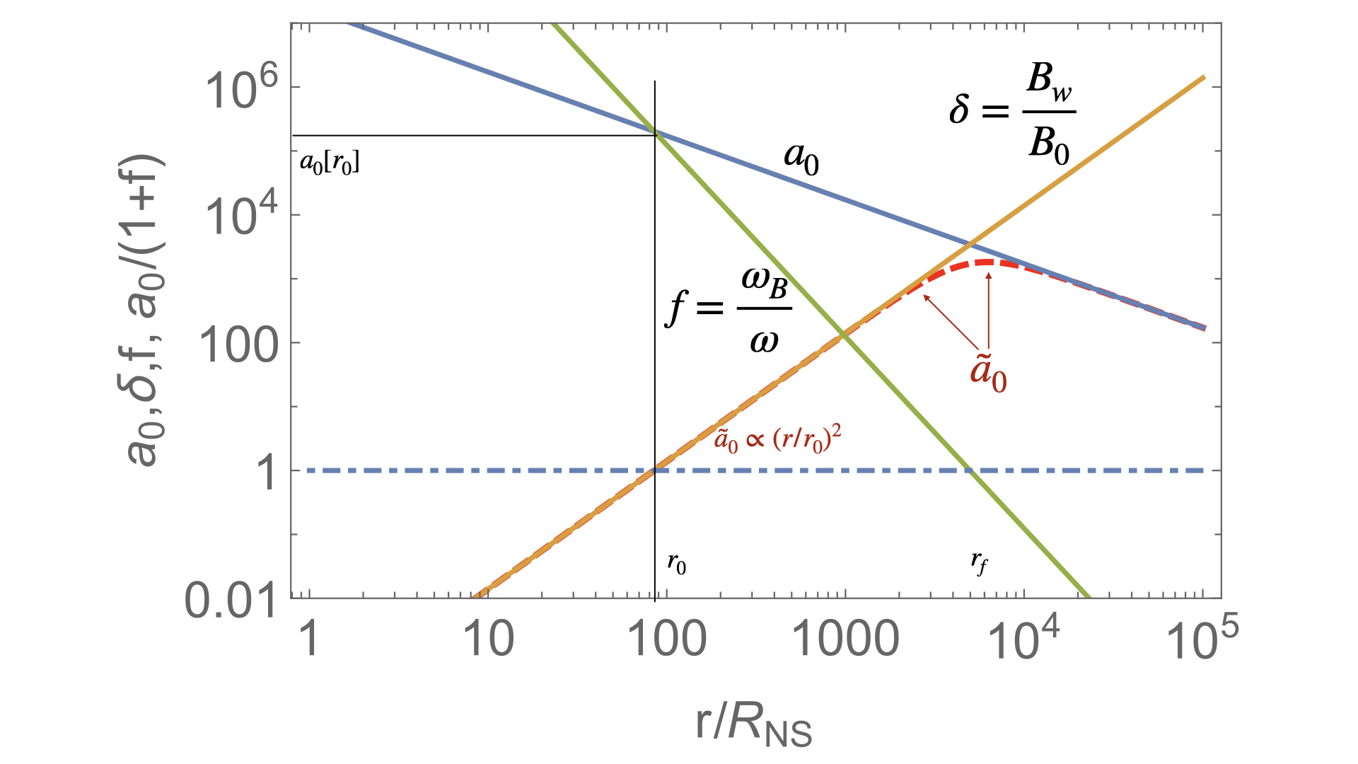
Figure 1: Evolution of basic parameters in the dipolar magnetosphere: nonlinearity parameter $a_{0}$, relative wave intensity $\delta=B_{w}/B_{0}$, ratio of frequencies $f=\omega_{B}/\omega$, and effective nonlinearity parameter $\tilde{a}_{0}=a_{0}/(1+f)$. Indicated are radii $r_{0}$ (where $\tilde{a}_{0}=1$), value of $a_{0}[r_{0}]$, and radius $r_{f}$ where $f=1$. Maximal value of $\tilde{a}_{0}^{(max)}\approx 1.8\times 10^{3}$ is reached approximately at $r_{f}$.

The key parameter $\tilde{a}_{0}$, Eq. (5), has a maximum (for dipole field) at

$$r/r_{0}=(2a_{0}[r_{0}])^{1/3}=2^{1/3}r_{f}\mbox{}$$

$$\tilde{a}_{0}^{(max)}=\frac{2^{2/3}}{3}a_{0}[r_{0}]^{2/3}$$ (15)

This estimates to

$$\left(\frac{r}{R_{NS}}\right)=b_{q}^{1/3}\left(\frac{c^{2}m_{e}}{\pi\hbar\nu}\right)^{1/3}=6\times 10^{3}\times b_{q}^{1/3}\mbox{}$$

$$\tilde{a}_{0}^{(max)}\approx 1.8\times 10^{3}\times b_{q}^{-1/3}$$ (16)

Parameter $\tilde{a}_{0}^{(max)}$, Eq. (16) is an important one. This is an estimate of the maximal total Lorentz factor, $\sim\tilde{a}_{0}^{(max),2}$, maximal parallel Lorentz factor, $\sim\tilde{a}_{0}^{(max)}$, and maximal transverse momentum $\sim\tilde{a}_{0}^{(max)}$.

For example, maximal values of the Lorentz factor are achieved at $r/r_{0}=(2a_{0}[r_{0}])^{1/3}$ and equals

$$\gamma_{p}=1+\frac{2^{1/3}}{9}a_{0}[r_{0}]^{4/3}$$ (17)

These values are large, and in the magnetospheres of magnetars would lead to large radiative losses, killing the EM pulse. We argue that these high values are not reached.

For the maximal $\tilde{a}_{0}^{(max)}$ to be reached with the magnetosphere, the period should be sufficiently long $P\geq 1$ sec. For shorter periods the value of $\tilde{a}_{0}^{(max)}$ is reached at the light cylinder, see (2). For mildly magnetized neutron stars, with regular surface field $\sim 10^{12}$ G ($b_{q}=0.02$), spinning with period $P\sim 20$ milliseconds, the value of $\tilde{a}_{0}^{(max)}$ can reach nearly $10^{4}$. It is not clear why FRB sources would fall into this special regime: higher surface field and faster spins push $\tilde{a}_{0}^{(max)}$ towards smaller values. For example, for quantum surface field $b_{q}=1$ and period of 10 milliseconds, $\tilde{a}_{0}^{(max)}$ is tiny, $\leq 1$.

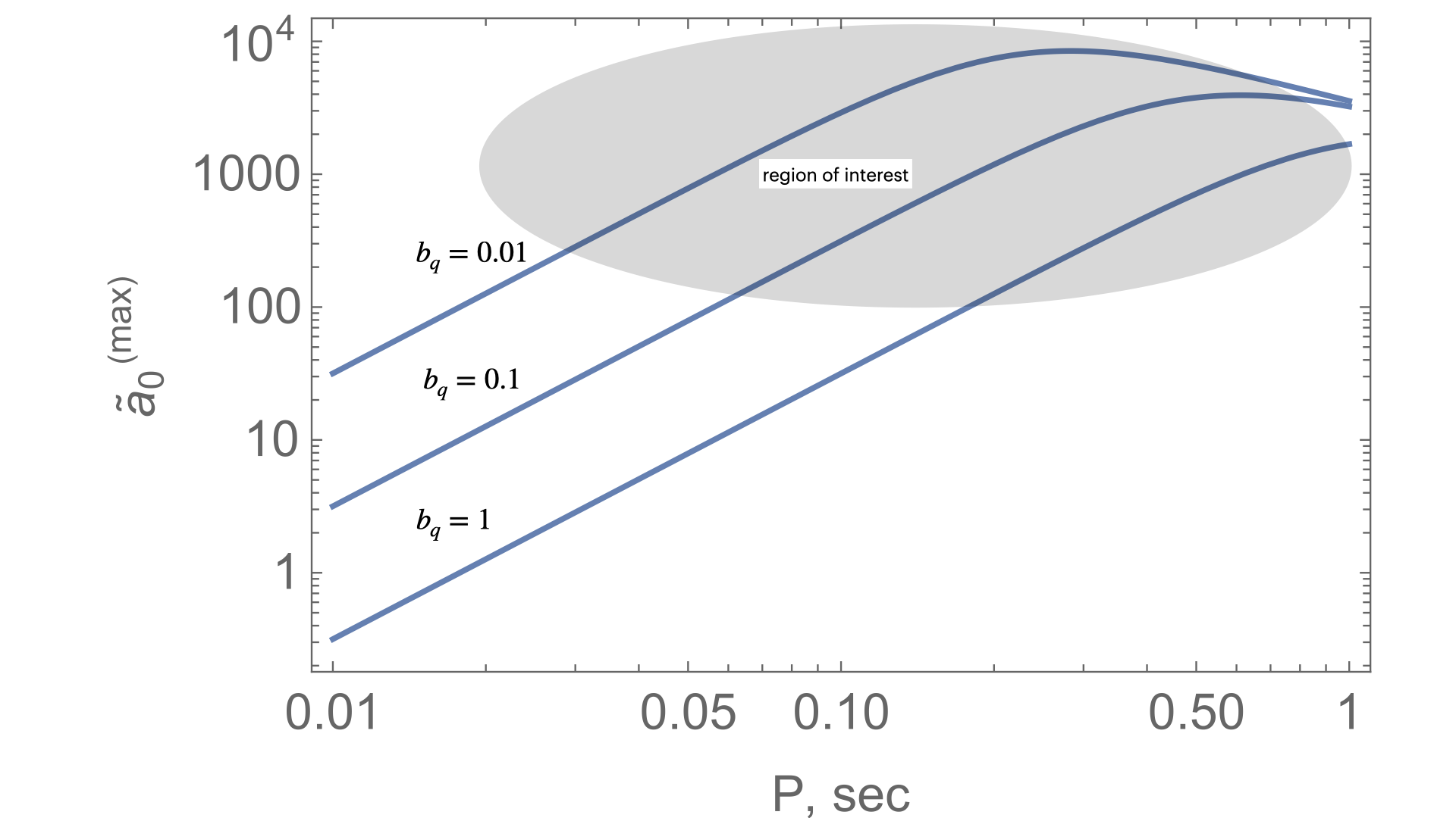
Figure 2: Maximal values of the non-linearity parameter $\tilde{a}_{0}$ reached at the light cylinder for spins faster than $P=1$ second (for slower spins see Eq. (16)), as function of the surface field $b_{q}=B_{NS}/B_{Q}$. Smaller magnetic fields are less efficient in suppressing $\tilde{a}_{0}$. ”Region of interest” indicates a set of parameters when wave’s nonlinearity may become large, $\geq 100$.

2.3 Post-eruption magnetic field lines are mostly radial, magnetic field increases in the outer parts of the magnetosphere

There are, qualitatively, three energy sources during FRB/magnetospheric eruption: (i) dynamical magnetic field; (ii) high energy emission; (iii) radio emission. Energetically, (i) $\gg$ (ii) $\gg$ (iii), so that the dominant effects to the distortion of the magnetic field come not from radiation, but from magnetospheric dynamics during the eruption.

The dynamical magnetic field is produced by a process that initiates magnetospheric eruption, e.g. , in an analogue to Solar Coronal Mass Ejection (CME). During CME a topologically isolated structure is injected into the magnetosphere, Lyutikov (2022); Sharma et al. (2023). Let’s assume that injection (generation of topologically disconnected magnetic structure) occurs near the stellar surface with the typical size $R_{CME,0}\leq R_{NS}$ and associated energy $E_{CME,0}$. An important parameter is the total magnetic energy of the magnetosphere,

$$E_{B,NS}\sim B_{0}^{2}R_{NS}^{3}$$ (18)

Naturally, the injected energy is much smaller than the total energy,

$$\eta_{CME}=\frac{E_{CME,0}}{E_{B,NS}}\leq 1$$ (19)

As the CME is breaking-out through the overlaying magnetic field, it does work on the magnetospheric magnetic field. At some point “detonation” occurs: when the total energy contained in the confining magnetic field exterior to the position of the CME ($\sim B_{0}^{2}R_{NS}^{6}r^{-3}$) becomes smaller than the CME’s internal energy (equivalently, when the size of the CME becomes comparable to the distance to the star). This occurs at some equipartition radius $r_{eq}$:

$$\frac{r_{eq}}{R_{NS}}\sim\frac{E_{B,NS}}{E_{CME,0}}=\eta_{CME}^{-1}\geq 1$$ (20)

Immediately after the generation of a CME the magnetosphere becomes open, with nearly radial magnetic field lines for $r\geq r_{eq}$.

For quantum surface field $E_{B,NS}\sim 2\times 10^{45}$ erg. The injected energy $E_{CME,0}$ is hard to estimate: the observed radio energy is an absolute lower limit. Much more energy is radiated in X-rays, even more is contained in the fields. (Also CME is losing energy to $pdV$ work as it breaks through the overlaying magnetic field Lyutikov, 2022; Sharma et al., 2023). It is conceivable that the relative injected energy may reach $\sim$ percent level of the total energy, $\eta_{CME}\sim 10^{-2}$. In this case, since beyond $r_{eq}$ the magnetic field decreases slower than dipole, $B\propto r^{-2}$ instead of $B\propto r^{-3}$, the the region where $f=\omega_{B}/\omega\geq 1$ will extend further. (Larger guide field suppresses particle’s transverse motion, see Fig. 4.)

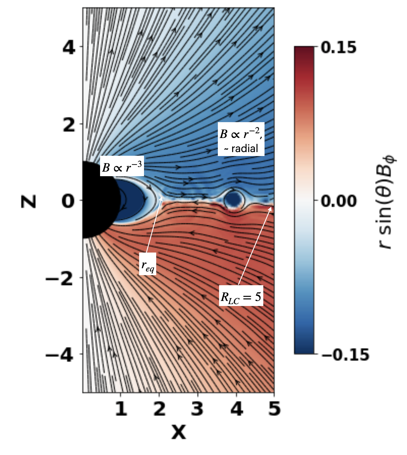
Figure 3: Post-flare opening of the magnetosphere (Sharma et al., 2023). Color is values $r\sin\theta B_{\phi}$, lines are poloidal field line. The spin parameter is $\Omega=0.2$, so that the light cylinder is at $R_{LC}=5$. Post-flare magnetosphere is open starting $r_{eq}\ll R_{LC}$, (20). Beyond $r_{eq}$ the magnetosphere has monopolar-like magnetic field structure.

Most importantly, beyond $r_{eq}$ the magnetic field becomes mostly radial. As a result, the electromagnetic waves generated close to the neutron star surface propagate nearly along the local field line. As we demonstrate in this work, this case does not suffer from strong radiative.

Finally, plasma is likely to stream out along the open field lines even before the FRB wave comes - this further freezes out wave-particle interaction, see Fig. 13.

3 Particle dynamics in circularly polarized wave propagating along guide field

3.1 Beam frame

Circularly polarized waves allow for exact analytical solutions, and thus provide benchmark for simulations and guidance for the more complicated linearly polarized case.

In the beam frame a force balance for a particle moving in electromagnetic field and guide magnetic field  reads

$$\gamma_{\pm}m_{e}v_{\pm}\omega=e(E_{w}\pm v_{\pm}B_{0})$$ (21)

where all quantities are positive: $\pm$ accounts for two directions of the background field/charge/polarization sign (speed of light is set to unity). Relations describe a charge which velocity at each moment (counter)-aligns with the magnetic field in the wave (Zeldovich, 1975). For a more general case see Roberts & Buchsbaum (1964); Kong & Liu (2007).

In dimensionless notations the motion of a particle in circularly polarized electromagnetic wave obeys

$$a_{0}=p_{0}\left|1+\frac{1}{\sqrt{1+p_{0}^{2}}}f\right|\mbox{}$$

$$\gamma_{0}=\frac{1}{\sqrt{1-v_{0}^{2}}}$$ (22)

(here $\omega$ is the wave frequency in the gyration frame), see Fig. 4. Quantity $f$ can be negative: two signs correspond to two polarizations (or two signs of charges). Absolute value $|...|$ ensures the definition of $a_{0}\geq 0$; crossing the resonant condition for the minus sign changes just the phases of the particles. Below in this section we drop the prime, with clear understanding that the quantities are measured in the plasma frame.

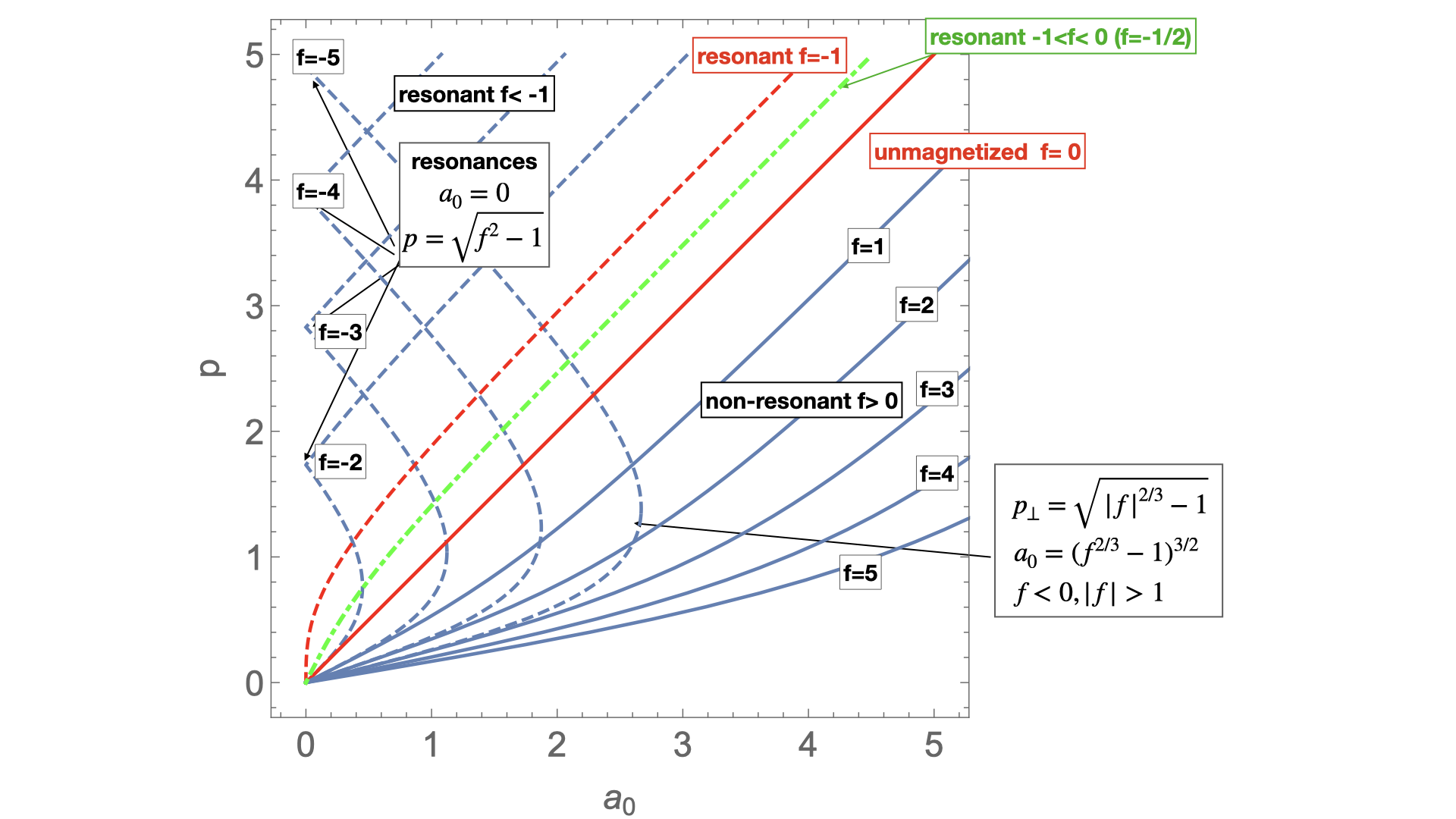
Figure 4: Particle’s transverse momenta in strong circularly polarized electromagnetic wave in external magnetic field. Wave intensity is parameterized by laser parameter $a_{0}$. Different curves correspond to different $f=\pm\omega_{B}/\omega$ (different charges or polarizations).

In (22) the values for $\gamma_{0}$ (for given $a_{0}$ and $|f|$) are different for two charges, especially near the cyclotron resonance $f\approx-1$. As we are not considering here the effects of cyclotron absorption, we assume below that $-f$ is not too close to unity.

In the case of strong electromagnetic pulse with $a_{0}\gg 1$, there are qualitatively three regimes: (i) small guide field $f\ll 1$, $p_{0}\sim a_{0}$; (ii) medium guide field $1\ll f\ll a_{0}$, $p_{0}\approx\delta\gg 1$ (in this case the transverse motion is still relativistic: a wave is sufficiently strong so that it accelerate particles to relativistic motion on time scale of $1/\omega_{B}$ ; (iii) dominant guide field $f\gg a_{0}$, $v_{0}\sim\delta\ll 1$ (in this case a particle just experiences E-cross-B drift).

3.2 Ponderomotive acceleration by circularly polarized wave propagating along the guide field

The above discussion in §3.1 omits the most important issue: the ponderomotive effects - how incoming wave modifies the properties of the plasma. As this is the most important part of the work, we give here detailed derivations.

Let a transverse circularly polarized wave of given strength $E_{w}$, frequency $\omega$ (measured in lab frame), non-linearity parameter $a_{0}$, propagating along guide magnetic field  $B_{0}{\bf e}_{z}$. Noting that

$$\partial_{t}\gamma=\frac{e}{m_{e}c^{2}}{\bf E}\cdot{\bf v}\mbox{}$$

$$\partial_{t}p_{z}=\frac{e}{c}\left.{\bf v}\times{\bf B}_{w}\right|_{z}$$ (23)

and expressing fields in terms of the vector potential

$${\bf E}_{w}=-\partial_{t}{\bf A}\mbox{}$$

$${\bf B}_{w}={\rm curl\,}{\bf A}$$ (24)

we find

$$\partial_{t}\gamma=-v_{x}\partial_{t}A_{x}-v_{y}\partial_{t}A_{y}\mbox{}$$

$$\partial_{t}p_{z}=v_{x}\partial_{z}A_{x}+v_{y}\partial_{z}A_{y}$$ (25)

Thus, the guide field does not enter the relations. Since $A=A(z-t)$, we find then

$$d_{t}(\gamma-p_{z}m_{e}c)=0$$ (26)

Switching to dimensionless notations and assuming that before the arrival of the wave a particle was at rest, we find

$$\gamma=1+p_{z}$$ (27)

We stress that for circularly polarized wave propagating along the magnetic field, this is valid for arbitrary guide field.

Thus (recall that $p_{0}$ is the transverse momentum, hence Lorentz invariant under a boost along $z$)

$$p_{z}=\frac{{\bf p}_{0}^{2}}{2}\mbox{}$$

$$\gamma=1+p_{0}^{2}/2=1+p_{z}\mbox{}$$

$$\gamma_{\parallel}=\frac{1}{\sqrt{1-\beta_{z}^{2}}}=\frac{1+p_{0}^{2}/2}{\sqrt{1+p_{0}^{2}}}=\frac{1+p_{z}}{\sqrt{1+2p_{z}}}\mbox{}$$

$$\gamma_{0}=\sqrt{1+p_{0}^{2}}\mbox{}$$

$$\beta_{z}=\frac{p_{0}^{2}}{2+p_{0}^{2}}\mbox{}$$

$$\tan\alpha_{p}=\frac{p_{0}}{p_{z}}=\frac{2}{p_{0}}$$ (28)

where $\alpha_{p}$ is pitch angle in lab frame. (Note that $\gamma_{\parallel}\neq\sqrt{1+p_{z}^{2}}$.) These relations establish connection between parallel motion acquired due to ponderomotive force and energy of the particle in the gyration/beam frame for circularly polarized wave, possibly propagating along guide magnetic field.

One remaining step is to connect $p_{z}$ (or $p_{0}$) to the waves’ parameters $a_{0}$ and $f$ at minus infinity, before interaction with a particle. Using invariance of $a_{0}=E_{w}/\omega$ and $\omega_{B}$, and Lorentz transformation of the frequency

$$\omega^{\prime}=(1-\beta_{\parallel})\gamma_{\parallel}\omega$$ (29)

(where now primes denote quantities measured in the beam frame) we arrive at

$$p_{0}=\frac{a_{0}}{1+f}\mbox{}$$

$$\gamma_{\perp}=\sqrt{1+p_{0}^{2}}=\sqrt{1+\left(\frac{a_{0}}{1+f}\right)^{2}}\mbox{}$$

$$p_{z}=\frac{a_{0}^{2}}{2(1+f)^{2}}\mbox{}$$

$$\gamma=1+\frac{a_{0}^{2}}{2(1+f)^{2}}\mbox{}$$

$$\beta_{z}=\frac{a_{0}^{2}}{2(1+f)^{2}+a_{0}^{2}}\mbox{}$$

$$\gamma_{\parallel}=\frac{1}{\sqrt{1-\beta_{z}^{2}}}=\frac{a_{0}^{2}+2(1+f)^{2}}{2(1+f)\sqrt{a_{0}^{2}+(1+f)^{2}}}=\frac{\gamma}{\gamma_{\perp}}\mbox{}$$

$$\tan\alpha=\frac{p_{0}}{p_{z}}=\frac{2(1+f)}{a_{0}}$$ (30)

We observe that the case with guide field is related to the no-guide field if we use

$$\tilde{a}_{0}=\frac{a_{0}}{1+f}$$ (31)

Then relations in magnetic field reduce to the same form as without guide field

$$p_{0}=\tilde{a}_{0}\mbox{}$$

$$p_{z}=\frac{\tilde{a}_{0}^{2}}{2}\mbox{}$$

$$\gamma=1+\frac{\tilde{a}_{0}^{2}}{2}\mbox{}$$

$$\tan\alpha=\frac{2}{\tilde{a}_{0}}$$ (32)

Importantly, relations (30-32) assume that the system is sufficiently large along the direction of propagation, so that a particle reaches the final steady state. As we show below, this is often not the case in magnetars’ magnetospheres.

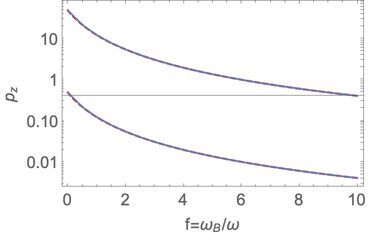
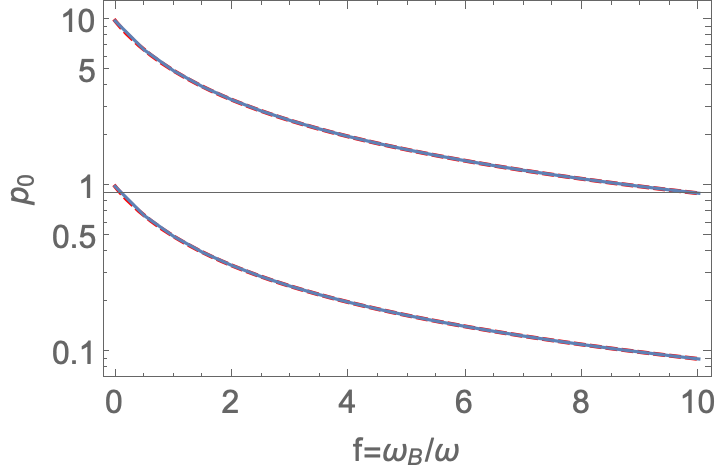
Figure 5: Ponderomotive acceleration by a circularly polarized electromagnetic  pulse propagating along the guide field, non resonant case $f>0$. Plotted is the axial momentum $p_{z}$ (left panel) and transverse momentum $p_{0}$ (right panel) as a function of $f=\omega_{B}/\omega$ ($\omega$ defined in the lab frame) for two cases: $a_{0}=1$ (bottom curves) and $a_{0}=10$ (top curves). Dashed line is analytical result, Eq. (30). Numerical and analytical curves nearly coincide. These plots serves to illustrate the numerical precision of the code, and to validate the analytics.

3.3 Ponderomotive surfing in constant guide field

Ponderomotive force has another important effect: in a system limited in size, the head part of the pulse, which is already non-linear but has local nonlinearity parameter much smaller than the pulse, will accelerate a particle to relativistic velocities along wave’s direction of propagation, so that it will take a long time for the bulk of the pulse to catch-up with the particle. We consider this effect next.

Consider a wave propagating along the field (see §7 for oblique case.) Assume that a pulse approaches a particle initially at rest at $z=0$. The pulse has maximal amplitude $a_{0}$ and ramp-up width $\delta z=\tau c$, Fig. 6. At each moment the axial velocity is

$$\beta_{z}=\frac{dz}{dt}=\frac{\tilde{a}(z)^{2}}{2+\tilde{a}(z)^{2}}$$ (33)

where $\tilde{a}(z)$ is the wave amplitude at the current location of the particle, Fig. 6. Equation (33) can be integrated for $z(t)$ assuming some given profile of the pulse (e.g. $\tanh(z-t)/\tau$).

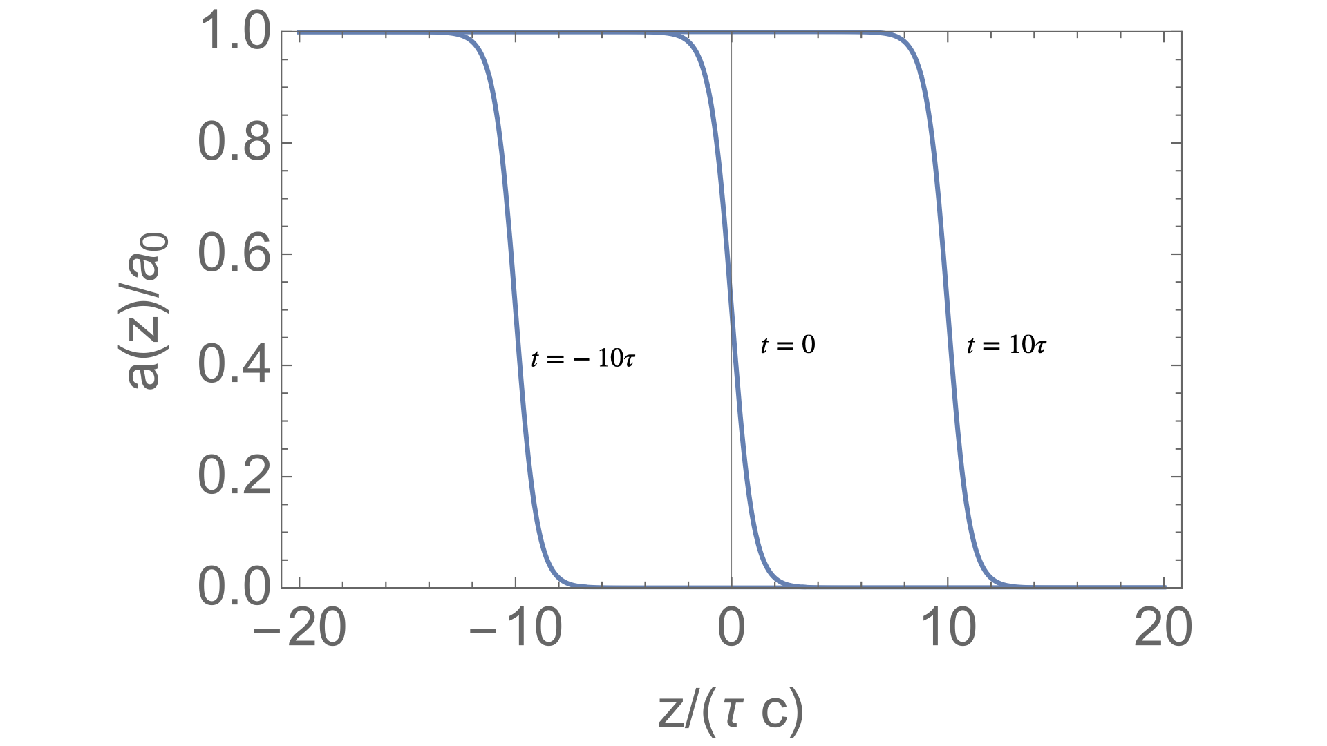
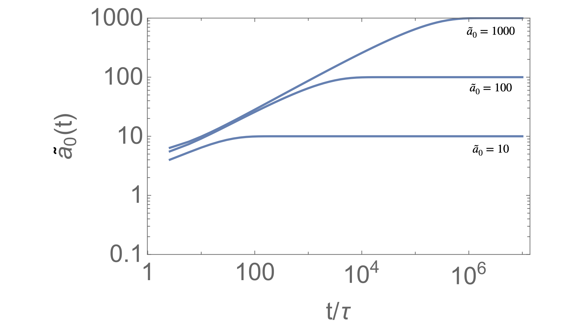
Figure 6: Left panel: An EM pulse with ramp-up width of $\tau=1$ propagates towards a particle initially at $z=0$. The pulse ponderomotively accelerates the particle along its direction of propagation. Right panel: Evolution of the non-linearity parameter $\tilde{a}_{0}(t)$ at the location of the particles for $\tilde{a}_{0}=10,\,100,\,1000$, constant guide field. Due to ponderomotive acceleration of the particle to $\gamma_{\parallel}\sim\tilde{a}_{0}$, the bulk of the pulse reaches the particle after a very long time, $\sim\tilde{a}_{0}^{2}\tau$.

What is important is not only the absolute value of the intensity $\tilde{a}_{0}$, but also temporal evolution of the non-linearity parameter at the location of the particle, Fig. 6 right panel. Due to ponderomotive acceleration of the particle to $\gamma_{\parallel}\sim\tilde{a}_{0}$, the bulk of the pulse reaches the particle after a very long time, $\sim(2/5)\tilde{a}_{0}^{2}\tau$.

As another measure, in Fig. 7 we plot a delay between the particle and the center of the pulse (located at $z=ct$). The delay becomes of the order of the width after time $\sim(2/5)\tilde{a}_{0}^{2}\tau$. (The center of the pulse, where local nonlinearity parameter is $\tilde{a}_{0}/2$ does not even overtake a particle before time $\approx\tau\gamma_{0}^{2}/10$.)

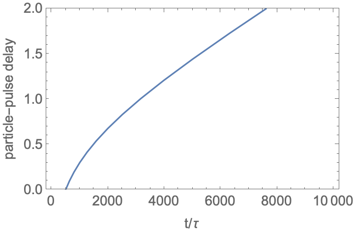
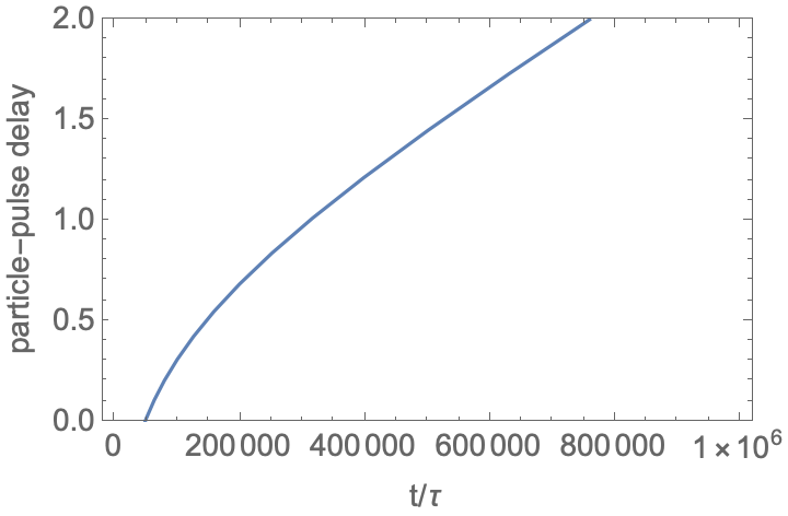
Figure 7: Pulse front - particle delay as function of time (measured in terms of pulse ramp-up time $\tau$ for $\tilde{a}_{0}=100$ (left) and $\tilde{a}_{0}=1000$ (right), constant guide field. The delay becomes of the order of unity after time $\sim(2/5)\tilde{a}_{0}^{2}\tau$.

3.4 Adiabatic force

The above relations omit an important effect: the adiabatic force that accelerates particles along decreasing magnetic field at the expense of transverse motion.

Adiabatic force can be written as (the parallel component is sometimes called the mirror force)

$$G_{\phi}=\pm\frac{\beta^{2}\gamma m_{e}c^{2}}{4}\frac{({\bf b}\nabla)B}{B}\sin 2\alpha\mbox{}$$

$$G_{z}=\mp\frac{\beta^{2}\gamma m_{e}c^{2}}{2}\frac{({\bf b}\nabla)B}{B}\sin^{2}\alpha$$ (34)

where ${\bf b}$ is unit vector along the magnetic field, $\alpha$ is pitch angle, and upper (lower) signs correspond to particle propagating towards (away from) the regions of increasing magnetic field. Since ${\bf G}\cdot{\bf v}=0$, the Lorentz factor $\gamma=$ constant. Adiabatic force can be thought of as $({\bf m}\cdot\nabla){\bf B}$ force, where ${\bf m}$ is the magnetic momentum.

Neglecting particular dependence of the value of the magnetic field on the polar angle,

$$\frac{({\bf b}\nabla)B}{B}=-\frac{1}{3r}$$ (35)

Where we chose axis $z$ along the local magnetic field, pointed away from the star, and we assumed that particles are moving away.

In dimensionless notations

$$\partial_{t}p_{\perp}=-\frac{\beta^{2}\gamma p_{\perp}p_{z}}{6\left(\gamma^{2}-1\right)r}\mbox{}$$

$$\partial_{t}p_{z}=\frac{\beta^{2}\gamma p_{z}^{2}}{6\left(\gamma^{2}-1\right)r}$$ (36)

Adiabatic force accelerates along the field at the expense of transverse motion.

To get a feeling of how the adiabatic force affects the dynamics, let’ us assume that it acts on time scales longer than pulse ramp-up time. In this case, at each radius there is ponderomotive force, so that total force balance reads

$$\partial_{r}p_{\perp}=-\frac{\beta^{2}\gamma p_{\perp}p_{z}}{6\left(\gamma^{2}-1\right)r}+\partial_{r}\tilde{a}_{0}\mbox{}$$

$$\partial_{r}p_{z}=\frac{\beta^{2}\gamma p_{z}^{2}}{6\left(\gamma^{2}-1\right)r}+\tilde{a}_{0}\partial_{r}\tilde{a}_{0}$$ (37)

In the region $r_{0}\ll r\ll r_{f}$, $\tilde{a}_{0}\approx(r/r_{0})^{2}$. Assuming relativistic motion $\gamma\gg 1$, and $p_{z}\gg p_{\perp}$

$$\partial_{r}p_{\perp}=-\frac{p_{\perp}}{6r}+\frac{2r}{r_{0}^{2}}\mbox{}$$

$$\partial_{r}p_{z}=\frac{p_{z}}{6r}+\frac{2r^{3}}{r_{0}^{4}}$$ (38)

with solutions

$$p_{\perp}=\frac{12}{13}\frac{r^{2}}{r_{0}^{2}}\mbox{}$$

$$p_{z}=\frac{12}{23}\frac{r^{4}}{r_{0}^{4}}$$ (39)

Thus, in the regime of short pulses, with ramp-up scale $\ll r$, the adiabatic force has $\sim 10\%$ effect on the particle dynamics, increasing parallel momentum and decreasing the transverse one. Qualitatively, since the losses are high powers of the transverse momentum, this will reduce the losses by about 50%. Our numerical results confirm this conclusion, Fig. 8.

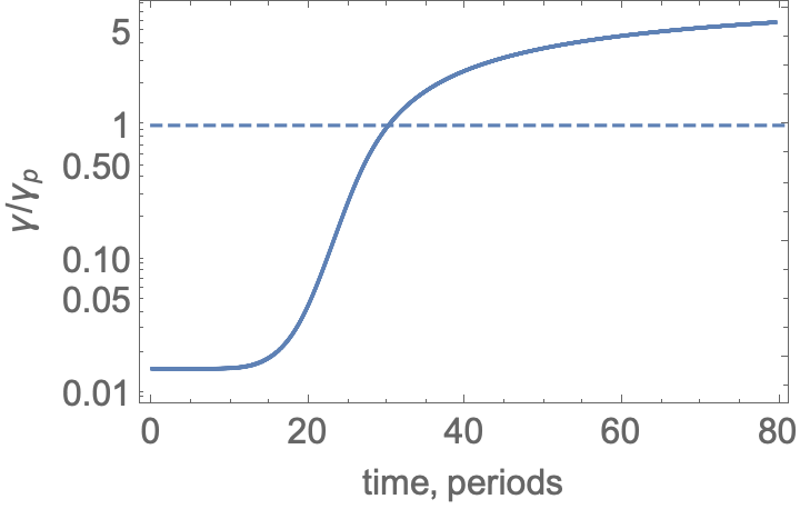
Figure 8: Effect of adiabatic acceleration by Gaussian pulse. Dashed curve: expected maximal Lorentz factor without effects of adiabatic acceleration, Eq. (17). This illustrates the importance of adiabatic acceleration. Initially, $a_{0}=f=100$, so $\gamma_{p}=66$. At time $t=0$ the peak of the pulse is at $-20$ wavelengths, rise time is $5$ wavelengths, scale of magnetic field decrease is 10 times the rise time. This confirms that adiabatic effects have about $10\%$ influence on particle dynamics

The adiabatic force helps somewhat particles to avoid losses, as it decrease transverse momentum (hence decreasing radiative losses) and increases parallel momentum (hence increasing the surfing time).

4 “Gone with the pulse”

Above we separately described various ingredients - overall particle dynamics in the beam frame, ponderomotive and adiabatic accelerations. Next we use these results to study particle dynamics within magnetars’ magnetospheres.

4.1 Ponderomotive acceleration in magnetars’ magnetospheres

First, we take semi-analytical account of ponderomotive acceleratrion in magnetars’ magnetospheres. We solve Eq. (33) taking into account both the structure of the pulse and spacial dependence of the parameter $\tilde{a_{0}}$. The following procedure is applied

• particle is seeded at a given radius

• An electromagnetic pulse of circularly polarized wave is launched from a much smaller radius. The pulse has a $\propto\tanh(r-t)/\tau$ profile with rump-up time.

• Pulse normalization follows evolution of the parameter $\tilde{a}_{0}$.

• We numerically integrate Eq. (33) for the location $z(t)$

In Fig. 9 we show evolution of the $\tilde{a_{0}}$ in the particle frame (as measured at the location of the particle) for different initial position of the particles. Particles located close to $r_{0}=100R_{NS}$ initially experience mild parallel acceleration, hence quickly overtaken by the head of the pulse and find themselves in the strong region of the wave (they do not experience much surfing on the rising part). Particles starting further out quickly gain large Lorentz factors, surf the front part of the pulse, and never experiences near-maximal value of $\tilde{a}_{0}$. Only particles located initially within few $r_{0}$ experience maximal wave’s intensity.

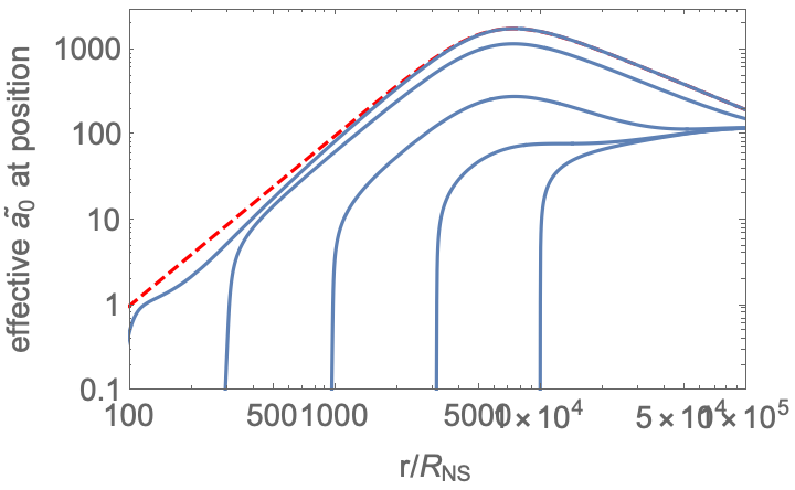
Figure 9: Non-linearity parameter $\tilde{a}_{0}$ at the location of a particle in dipolar-like magnetosphere  for different initial positions of a particle, subject to a pulse $\propto\tanh(r-t)/\tau$ with rump-up time of $\tau=10R_{NS}/c$. Red line: local value of $\tilde{a}_{0}$. This illustrates that particles initially located at $\geq$ few $r_{0}$ do not experience full waves’ nonlinearity do to effect of surfing.

Qualitatively, in the region $r\geq r_{0}$ (recall that $r_{0}\sim 10^{2}R_{NS}$).

$$\tilde{a}_{0}\approx\left(\frac{r}{r_{0}}\right)^{2}\mbox{}$$

$$\gamma_{\parallel}\approx\frac{\tilde{a}_{0}}{2}$$ (40)

For a pulse with rise time $\tau\sim R_{NS}/c$ the distance $r_{over}$ the pulse would overtake the particle estimates to

$$r_{over}\sim c\tau\gamma_{\parallel}^{2}$$ (41)

The condition $r_{over}\sim c/\Omega$ then gives

$$\gamma_{\parallel}\sim\tilde{a}_{0}^{(eff)}/2=(\tau\Omega)^{-1/2}=70\sqrt{P}$$ (42)

where period $P$ is in seconds. The parameter

$$\tilde{a}_{0}^{(eff)}\sim 10^{2}\sqrt{P}$$ (43)

is a typical nonlinearity parameter that a particle experiences while surfing the pulse. It is an order of magnitude smaller than would be inferred without ponderomotive acceleration, Eq. 16).

4.2 Ponderomotive and adiabatic acceleration

The above results, integration of the parallel momentum (33), did not take adiabatic acceleration into account. To further clarify the situation, in Fig. 10 numerically integrate particles motion in the field of incoming pulse, in inhomogenous decreasing guide field. This is done using in-house built Boris-based pusher (Boris & Roberts, 1969; Birdsall & Langdon, 1991). In the simulations a particle is initially located 4 rump-up scales ahead of the $\tanh(r-t)/\tau$ with rump-up scale $\tau=5$ wavelength. At the initial location of the particle the wave intensity correspond to $\tilde{a}_{0}=100$. Four different parameters $f$ are shown: $f=100,10,1$. These different values of $f$ mimic different initial locations in the magnetosphere: $f=100$ corresponds to $r=r_{0}$, $f=1$ corresponds to $r=r_{f}$. We plot the delay between a local position of a particle and a middle of the pulse, where intensity is half the local maximum.

Our numerical results indicate that combined effects of ponderomotive and adiabatic acceleration hugely increase over-take time. We observe that for $f=100$ (lower curve, equivalent to starting at $r=r_{0}$) the head of the pulse quickly passes the particle (since initially its velocity is only mildly relativistic). As a result a particle quickly “feels” the full intensity of the wave. In contrast, the head of the pulse never overtakes a particle located midway between $r_{0}$ and $r_{f}$ (middle curve), or further out. This demonstrates that due to a limited radial extent a particle may never reach the terminal state with local $p_{0}=\tilde{a}_{0}$, as predicted by (30).

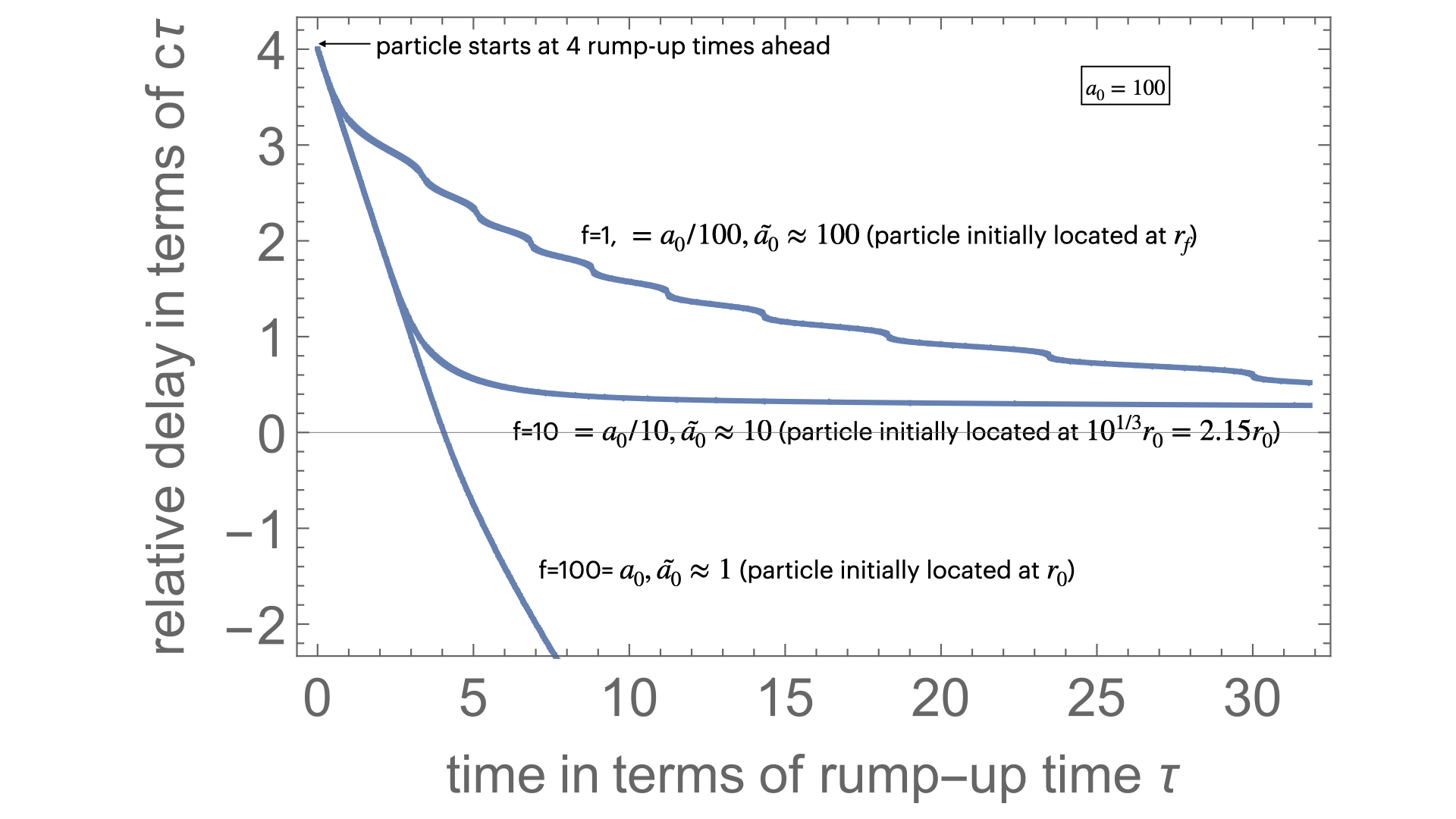
Figure 10: Delay times of “particle-center of the pulse” for different initial $f=\omega_{B}/\omega$ parameters (effective different initial locations). Calculations start at four rump-up times, $\tanh$ profile the pulse, magnetic field changes on 10 ramp-up scale.

In all cases particles initially located beyond $r_{0}$ quickly acquire relativistic velocities. For particles near $r_{0}$ these relativistic velocities are not sufficient to escape the full nonlinearity of the wave, bit still, $v\sim c$. Thus, the leading part of the wave will clear particles from the magnetosphere

4.3 Dissipated energy

Let us estimate the expected energy loss by the wave, assuming that the frontal particles loses all the energy it acquired in the wave As figure (11) indicates, only particle in a narrow layer near $r_{0}$ (where $\tilde{a}_{0}$ just becomes of the order of unity) experience large acceleration. Most of the magnetospheres surfs the wave and do reach very large energies. As an estimate of the dissipated power we can use

• volume $V\sim 4\pi r_{0}^{2}\times 3r_{0}$ (assuming thickness of $3r_{0}$).

• Lorentz factor  $\gamma\sim\left(\tilde{a}_{0}^{(max)}\right)^{2}/2$

• density $\kappa n_{GJ}$ ($\kappa\sim 10^{5}$ is multiplicity, $n_{GJ}$ is the Goldreich & Julian (1970) density).

• period $P$ in seconds

We find for dissipated energy $E_{dis}$

$$E_{dis}=5\times 10^{36}\left(\frac{\kappa}{10^{5}}\right)P^{-1}\,{\rm erg}$$ (44)

A safely mild value, much smaller than the total energy of the FRB (6).

Fig. 9 also indicates that the bulk of the particles in the magnetosphere  experience $\tilde{a}_{0}\sim 100$ (hence $\gamma\sim 5\times 10^{3}$). The total associated energy within the light cylinder is then $\sim 5\times 10^{33}$ ergs. Thus, most of the energy the wave spends on cleaning the magnetospherenear $r\sim r_{0}$.

Finally, in Fig. 11 we plot the non-linearity parameter $\tilde{a}_{0}$ at the location of a particle in dipolar-like $B\propto r^{-3}$ and monopolar-like $B\propto r^{-2}$ scaling of the guide field. The rise time of the pulse is assumed to be very short $R_{NS}/c=30$ micro-seconds. Maximum value of the nonlinearity parameter at the location of the particle can reach $\sim 10^{3}$, but only for sufficiently slow spins $P\geq 100$ msec. If the magnetosphere is modified by the ejected CME to have a monopolar-like structure, the maximal non-linearity parameter that a particle experiences is only few times $10^{2}$. Longer rump-up times will further stretch the curves

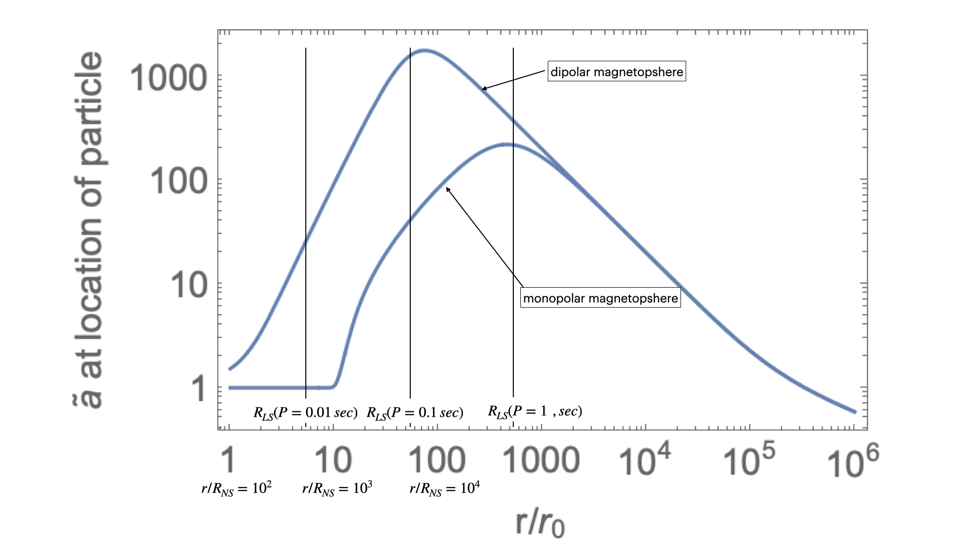
Figure 11: Non-linearity parameter $\tilde{a}_{0}$ at the location of a particle in dipolar-like and mono-polar-like scaling of the guide field. A particle is tracked from the point $r=r_{0}=10^{2}R_{NS}$, Eq. (12), where $\tilde{a}_{0}$ first becomes unity. Vertical lines indicate location of the light cylinder for different periods $P=0.01,\,0.1,\,1$ second. The assumed rise-time of the FRB pulse is $R_{NS}/c=30$ microseconds.

5 Different polarization and obliquity

We also considered effects of wave’s oblique propagation with respect to magnetic field, as well as various polarization. Taking care of the ponderomotive acceleration of particles as the FRBs’ wave comes into plasma is most important. The code reproduces well analytical results for ponderomotive acceleration, Fig. 5. We run a few simulations for different angles of propagation with respect to the magnetic field, and different polarizations.

Besides the parameters $a_{0},\,\delta$ and $f$ defined above, there is angle $\theta$ between the direction of wave propagation and the external magnetic field and the polarization angle of the wave $\phi$ (for $\phi=0$ the electric field of the wave is in the plane defined by the direction of wave propagation and the external magnetic field, this is then the O-mode, for $\phi=\pi/2$ the magnetic field  of the wave is in the plane defined by the direction of wave propagation and the external magnetic field, this is then the X-mode). In this particular section, the wave intensity is also modulated by a Gaussian envelope (adiabatic switching on and off), Fig 13.

We observe two types of wave-particle interaction occur. First, for exactly parallel propagation, as a wave packet come in, it accelerate a particle along the external magnetic field by the ponderomotive force, plus a particle oscillates in the combined field of the wave and the external magnetic field. This motion is reversible: a particle comes back to rest after the wave have left (if radiation reaction is neglected). Second, for oblique propagation, in a sufficiently strong wave a particle may occasionally experience DC-type acceleration (Beloborodov, 2021). The acceleration is of the diffusive type: occasionally a particle efficiently surfs the wave gaining energy. Appearance of regions with $E\geq B$ greatly helps this type of acceleration, but is not needed: the O-mode, where $B$ is always larger than $E$ also shows this type of acceleration. This second type of wave-particle energy exchange it dissipative: after the wave has left, the particle retains some energy. Thus this reduces the wave intensity.

We find that the dissipative interaction is highly dependent on the obliquity and polarization. The particular case considered by Beloborodov (2021), that of an X-mode propagating perpendicular to the magnetic field is the most extreme, the most dissipative one. For more general geometry and polarization, the resulting energy exchange is orders-of-magnitude smaller. Any pre-wave parallel motion further reduces the losses.

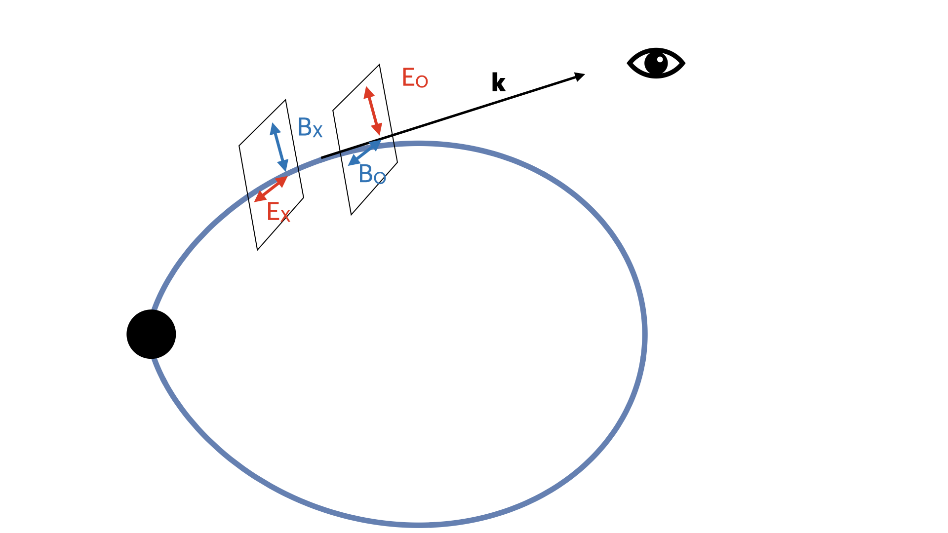
Figure 12: Two polarizations add differently with the external magnetic field. For the X-mode the magnetic field of the wave is in the plane of the dipolar field; the total magnetic field at some moments may become smaller than the electric field. For the O-mode the magnetic field of the wave is perpendicular to the dipolar field; the total magnetic field  is always larger than the electric field.

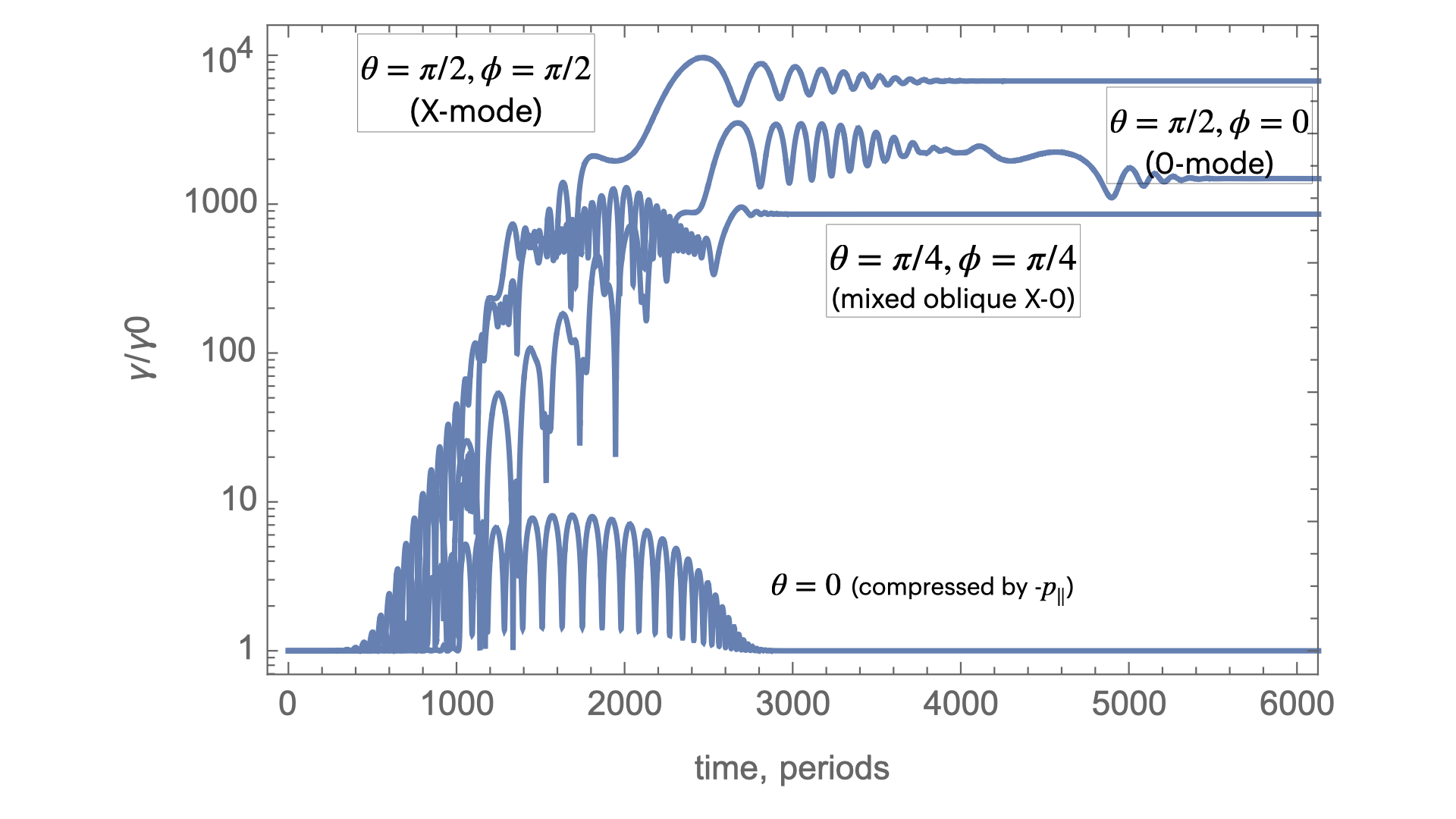
ı

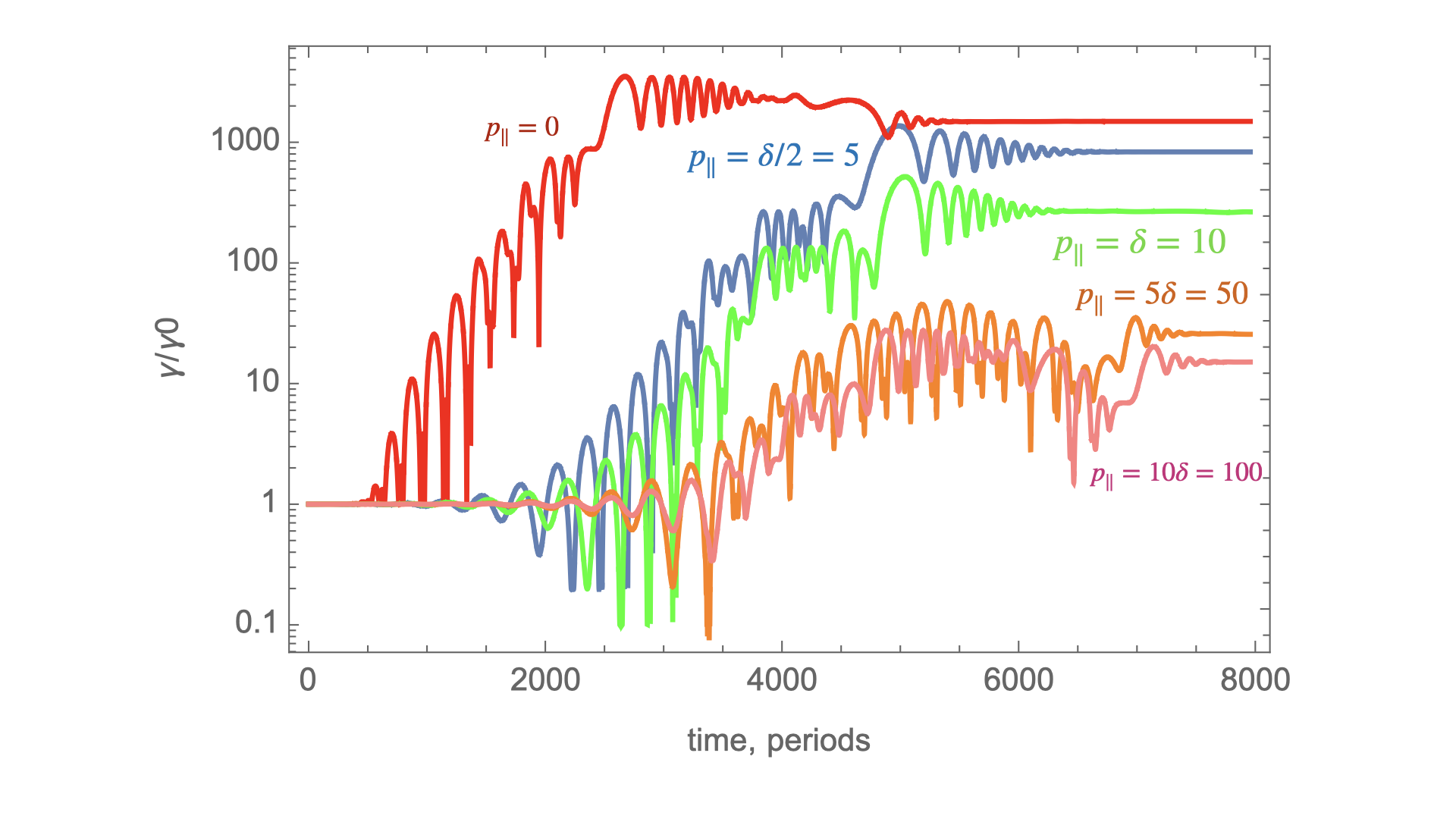
Figure 13: Left panel: Evolution of Lorentz factor for a laser pulse with $\delta=10$, $f=100$ for different directions of propagation with respect to the magnetic field (angle $\theta$) and different polarization (angle $\phi$).In the parallel case $\theta=0$ the ponderomotive force accelerates the particle along magnetic field so that it surfs the wave for a very long time; to shorten dynamical time the particle was injected with momentum against the wave. Most importantly, in the parallel case there is no dissipation: after the wave packet passes by, the particle energy returns to the initial Lorentz factor. Both for X-mode and O-mode periods of just oscillations in the field are intermitted with “surfing” - a sudden increase of particle’s energy. The X-mode is most prone to dissipation/particle acceleration. The O-mode experiences an order-of-magnitude smaller dissipation. Parallel propagation is completely ideal. Right panel: Influence of the initial outward momentum. Evolution of the relative Lorentz factor of particle moving initially along magnetic field  with various Lorentz factors. Parameters: $\delta=10$, $f=100$, $\theta=\pi/4$, $\phi=\pi/4$.

Our numerical simulations imply

• X-mode propagating perpendicular to the magnetic field indeed suffers heavy absorption. This is the case considered by Beloborodov (2021). In the X-mode, the guide magnetic field  periodically subtracts from the wave’s magnetic field  leading to appearance $E\geq B_{tot}$ and efficient particle acceleration

• O-mode, for which $E\leq B$ always, also shows occasional burst of particle’s acceleration. In these cases the particles nearly surfs the electric field of the wave. But overall, the energy gained by a particle in the O-mode is an order of magnitude smaller that in the X-mode.

• Exactly parallel propagation is purely non-dissipative

• initial parallel motion away from the pulse greatly reduce dissipative effects.

6 Effects of initial parallel velocity

Opening of the magnetosphere, §2.3, will also generate radial plasma outlfow. We did a series of numerical runs that included initial parallel motion of a particle, Fig 13. Our conclusion is that initial parallel momentum greatly deacreses the efficiency of wave-particle interaction.

To estimate the effects of initial parallel momentum, we note that instead of (27) we have

$$\gamma-p_{z}=\gamma_{i}-p_{i}\mbox{}$$

$$\gamma_{i}=\sqrt{1+p_{i}^{2}}$$ (45)

where $\gamma_{i}$ and $p_{i}$ are initial Lorentz factor and mmentum along the field (away from the diretion of pulse propagation).

We find

$$p_{z}=\frac{1+p_{0}^{2}/2}{\gamma_{i}-p_{i}}-\gamma_{i}\approx(1+p_{0}^{2})\gamma_{i}\mbox{}$$

$$\gamma=\sqrt{1+p_{0}^{2}+\frac{\left(1+p_{0}^{2}/2-\gamma_{i}^{2}+\gamma_{i}p_{i}\right){}^{2}}{\left(\gamma_{i}-p_{i}\right){}^{2}}}\approx(1+p_{0}^{2})\gamma_{i}\mbox{}$$

$$\beta_{z}=p_{z}/\gamma\approx 1-\frac{1}{2(1+p_{0}^{2})\gamma_{i}^{2}}\mbox{}$$

$$\gamma_{\parallel}\approx\sqrt{(1+p_{0}^{2})}\gamma_{i}$$ (46)

The resonant condition (29) now gives, approximately, $\gamma_{i}\gg 1$,

$$p_{0}=\frac{a_{0}}{1+\gamma_{i}^{3/2}/(2\sqrt{2})f}\approx\gamma_{i}^{-3/2}\frac{a_{0}}{f},$$ (47)

showing that even mild values of $\gamma_{i}\sim$ few strongly suppress wave-particle interaction. Qualitatively, initial parallel motion with Lorentz factor $\gamma_{i}$ away from the star reduces the inital wave’s frequency in the particle frame, leading to higher effective $f$, and decrease of $\tilde{a}_{0}$.

7 Self-cleaning

As discussed above the most important dissipation occurs on particles that start from $r\sim r_{0}\sim 10^{2}R_{NS}$ (where $\tilde{a}_{0}\sim 1$), and experience largest dissipation at $r\sim r_{f}\sim 5\times 10^{3}R_{NS}$ where $f\sim 1$. As the ratio $r_{f}/r_{0}\gg 1$, the field geometry (with respect to wave’s propagating) may change substantially.

For mildly oblique propagation, $\theta\neq 0$, the surfing effect is reduced. For small angles of propagation a particle still surfs the wave for a long time $\sim 1/\theta$. At large angles, $\theta\sim 1$, a new effect appears - self cleaning, Fig. 14. Consider a pulse of finite transverse dimensions. For oblique magnetic field the leading part of the pulse would ponderomotively push the plasma particles along the local magnetic field. For oblique magnetic field, particles will stream sideways, clearing the path for the main part of the pulse.

Fig. 14, right panel, shows the results of simulations. Plotted is a transverse (sideway) displacement of a particle as a function of magnetic obliquity $\theta$ for several parameters of wave intensity $\delta$ and the frequency parameter $f$. Overall, the displacement shows the expected $\propto\sin\theta\cos\theta$ dependence. Except for the case of mild wave in high magnetic field  ($\delta=1,\,f=10$), the curves approximately match, since the motion along the field becomes relativistic.

In addition, intermediate cases show relatively high random variations in the final displacement. This generally consistent with the previously discusses concept that particles’ trajectories can be mildly stochastic.

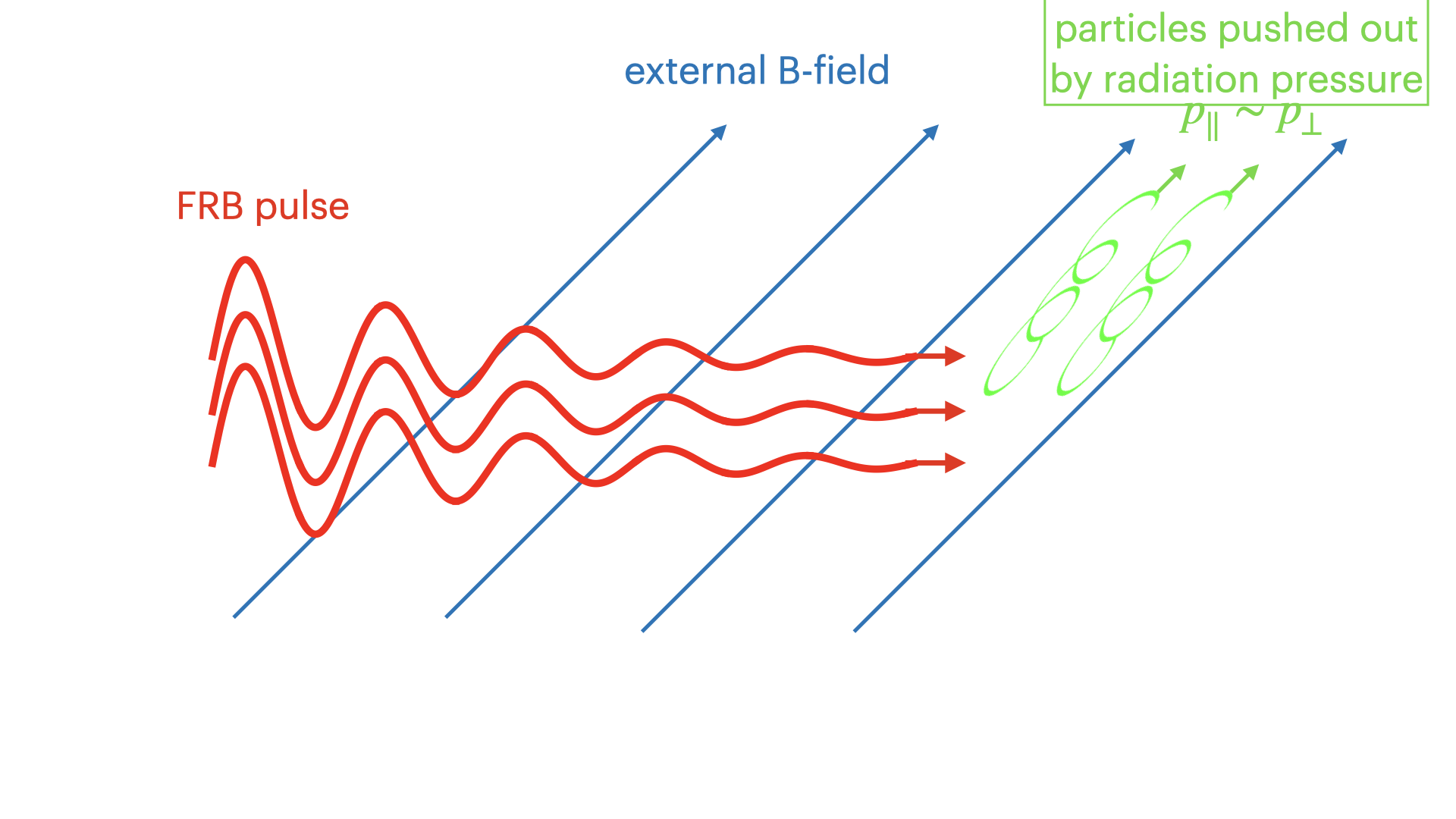
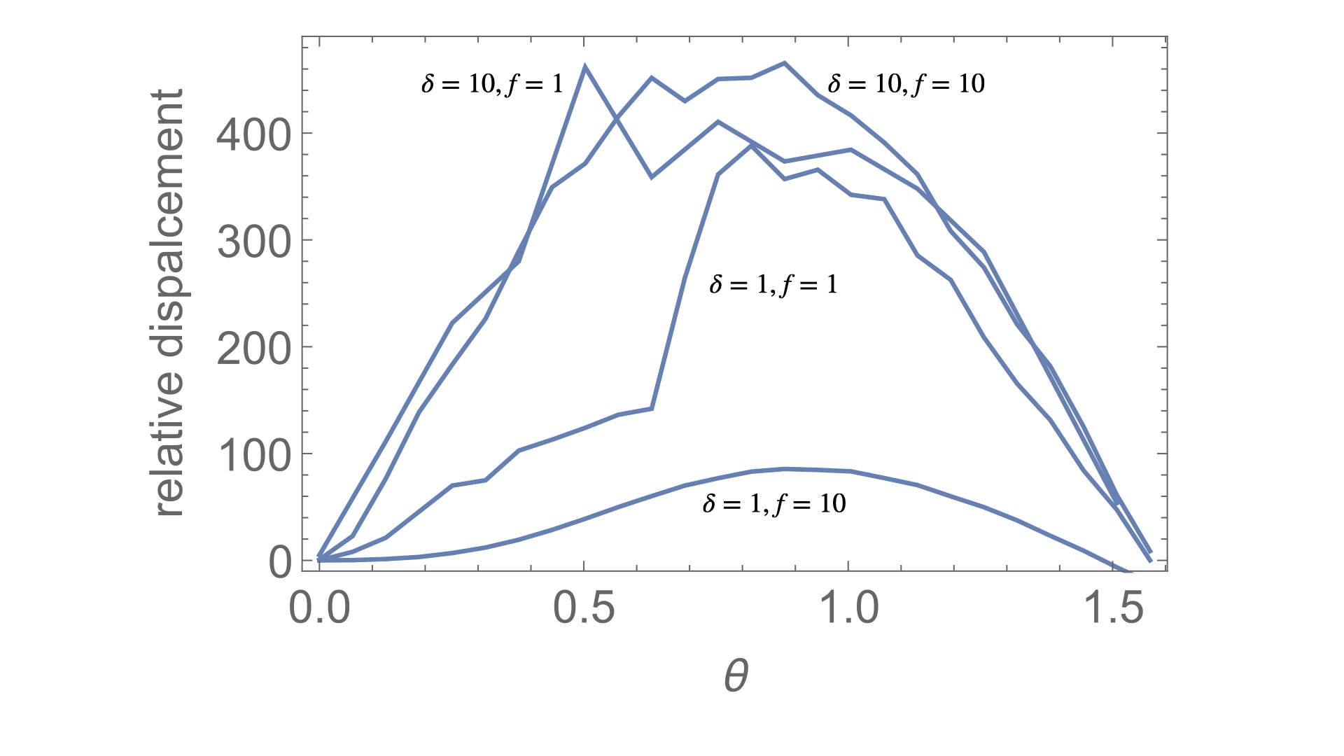
Figure 14: Self-cleaning. Left panel: cartoon how the leading part of the pulse, propagating at oblique angles to the magnetic field, ponderomotively pushes the particles away from the propagation path. The bulk of the pulse then propagates through nearly vacuum, and does not experience dissipation. Right panel: sideway displacement as function of the angle between the waves’ propagation and magnetic field.

8 Discussion

In this work we consider escape of high brightness radiation from magnetars’ magnetospheres, and conclude that there are multiple ways to avoid nonlinear absorption. First, strong non-linear effects are expected in a limited range of parameters, around surface magnetic fields of $\sim 10\%$ of critical and spin periods of $\sim$ tens of millisecond. Larger magnetic fields, and shorter periods limit the effective non-linearity parameter to $\tilde{a}_{0}\leq 10^{2}$, see Fig. 2.

In the “region of interest”, we find that ponderomotive and parallel-adiabatic acceleration of particles. are most important. In a mildly strong leading part of the wave, particles quickly get large parallel momenta - this effectively freezes the interaction. Roughly speaking, in order to obtain transverse momentum $\sim p_{0}$, a particle needs to serf for time $\sim p_{0}^{2}\tau$, where $\tau$, is a rump-up time of the electromagnetic pulse. In the inner parts of the magnetosphere, the value of $p_{0}$ is suppressed by the guide magnetic field, so a pulse passes through quickly, bit does not shake the particles much. Further out, where a stationary particle could have been accelerated to a large Lorentz factor, it never happens because a particle is surfing the pulse and remains at locally low non-linearity parameter, before escaping magnetosphere.

All these issues are further overwhelmed by the parallel large Lorentz factor along the newly opened magnetic field lines, possibly initiated by the opening of the magnetosphere  during a CME. Large parallel momentum reduces $\delta=B_{w}/B_{0}$ in the particles’s frame, and leads to further freezing of the wave-particle dynamics.

Other points are: (i) the O-mode (which never has regions $E\geq B$ is much less prone to dissipation (but particles in the wave still experience occasional energy boost, draining wave’s energy); (ii) quasi-parallel propagation is intrinsically non-dissipative; (iii) magnetospheric dynamics during magnetar’s explosions ensures that the magnetic field becomes nearly radial beyond some distance - smaller than the light cylinder and dependent on the power of the explosion, see Eq. (20); as a result the electromagnetic pulse propagates nearly along the magnetic field; (iv) initial mildly relativistic velocity along the field, away from the star further reduces particles’ losses; (iv) leading part of the pulse may push the plasma sideways, clearing the path for the main part of the pulse.

We conclude that the case considered by Beloborodov (2021, 2022, 2023), X-mode propagating equatorially across magnetic field, is extreme, and is not indicative of the general situation. That is a specific case of no-surfing.

In the approach of Golbraikh & Lyubarsky (2023), the energy density of the waves and their frequency (the transformation rate) should be calculated in plasma frame, which is flying away with large Lorentz factor. In that frame the wave’s energy density is down by induced parallel Lorentz factor $\gamma_{\parallel}^{2}$ and frequency is down by $\gamma_{\parallel}$ , so total reduction of the efficiency of nonlinear interaction is $\sim\gamma_{\parallel}^{3}$.

This work had been supported by NASA grants 80NSSC17K0757 and 80NSSC20K0910, NSF grants 1903332 and 1908590. I would like to thank Alexey Arefiev, Andrei Beloborodov, Pawan Kumar, Mikhail Medvedev, Kavin Tangtartharakul, Chris Thompson, and Bing Zhang for discussions.

9 Data availability

The data underlying this article will be shared on reasonable request to the corresponding author.

References

- Akhiezer et al. (1975) Akhiezer, A. I., Akhiezer, I. A., Polovin, R. V., Sitenko, A. G., & Stepanov, K. N. 1975, Oxford Pergamon Press International Series on Natural Philosophy, 1
- Beloborodov (2017) Beloborodov, A. M. 2017, ApJ, 843, L26
- Beloborodov (2021) —. 2021, ApJ, 922, L7
- Beloborodov (2022) —. 2022, Phys. Rev. Lett., 128, 255003
- Beloborodov (2023) —. 2023, arXiv e-prints, arXiv:2307.12182
- Birdsall & Langdon (1991) Birdsall, C. K., & Langdon, A. B. 1991, Plasma Physics via Computer Simulation
- Bochenek et al. (2020) Bochenek, C. D., Ravi, V., Belov, K. V., Hallinan, G., Kocz, J., Kulkarni, S. R., & McKenna, D. L. 2020, Nature, 587, 59
- Boris & Roberts (1969) Boris, J. P., & Roberts, K. V. 1969, Journal of Computational Physics, 4, 552
- CHIME/FRB Collaboration et al. (2020) CHIME/FRB Collaboration, Andersen, B. C., Bandura, K. M., Bhardwaj, M., Bij, A., Boyce, M. M., Boyle, P. J., Brar, C., Cassanelli, T., Chawla, P., Chen, T., Cliche, J. F., Cook, A., Cubranic, D., Curtin, A. P., Denman, N. T., Dobbs, M., Dong, F. Q., Fandino, M., Fonseca, E., Gaensler, B. M., Giri, U., Good, D. C., Halpern, M., Hill, A. S., Hinshaw, G. F., Höfer, C., Josephy, A., Kania, J. W., Kaspi, V. M., Landecker, T. L., Leung, C., Li, D. Z., Lin, H. H., Masui, K. W., McKinven, R., Mena-Parra, J., Merryfield, M., Meyers, B. W., Michilli, D., Milutinovic, N., Mirhosseini, A., Münchmeyer, M., Naidu, A., Newburgh, L. B., Ng, C., Patel, C., Pen, U. L., Pinsonneault-Marotte, T., Pleunis, Z., Quine, B. M., Rafiei-Ravandi, M., Rahman, M., Ransom, S. M., Renard, A., Sanghavi, P., Scholz, P., Shaw, J. R., Shin, K., Siegel, S. R., Singh, S., Smegal, R. J., Smith, K. M., Stairs, I. H., Tan, C. M., Tendulkar, S. P., Tretyakov, I., Vanderlinde, K., Wang, H., Wulf, D., & Zwaniga, A. V. 2020, Nature, 587, 54
- Golbraikh & Lyubarsky (2023) Golbraikh, E., & Lyubarsky, Y. 2023, arXiv e-prints, arXiv:2309.09218
- Goldreich & Julian (1970) Goldreich, P., & Julian, W. H. 1970, ApJ, 160, 971
- Hurley et al. (2005) Hurley, K., Boggs, S. E., Smith, D. M., Duncan, R. C., Lin, R., Zoglauer, A., Krucker, S., Hurford, G., Hudson, H., Wigger, C., Hajdas, W., Thompson, C., Mitrofanov, I., Sanin, A., Boynton, W., Fellows, C., von Kienlin, A., Lichti, G., Rau, A., & Cline, T. 2005, Nature, 434, 1098
- Kong & Liu (2007) Kong, L.-B., & Liu, P.-K. 2007, Physics of Plasmas, 14, 063101
- Li et al. (2021) Li, C. K., Lin, L., Xiong, S. L., Ge, M. Y., Li, X. B., Li, T. P., Lu, F. J., Zhang, S. N., Tuo, Y. L., Nang, Y., Zhang, B., Xiao, S., Chen, Y., Song, L. M., Xu, Y. P., Liu, C. Z., Jia, S. M., Cao, X. L., Qu, J. L., Zhang, S., Gu, Y. D., Liao, J. Y., Zhao, X. F., Tan, Y., Nie, J. Y., Zhao, H. S., Zheng, S. J., Zheng, Y. G., Luo, Q., Cai, C., Li, B., Xue, W. C., Bu, Q. C., Chang, Z., Chen, G., Chen, L., Chen, T. X., Chen, Y. B., Chen, Y. P., Cui, W., Cui, W. W., Deng, J. K., Dong, Y. W., Du, Y. Y., Fu, M. X., Gao, G. H., Gao, H., Gao, M., Gu, Y. D., Guan, J., Guo, C. C., Han, D. W., Huang, Y., Huo, J., Jiang, L. H., Jiang, W. C., Jin, J., Jin, Y. J., Kong, L. D., Li, G., Li, M. S., Li, W., Li, X., Li, X. F., Li, Y. G., Li, Z. W., Liang, X. H., Liu, B. S., Liu, G. Q., Liu, H. W., Liu, X. J., Liu, Y. N., Lu, B., Lu, X. F., Luo, T., Ma, X., Meng, B., Ou, G., Sai, N., Shang, R. C., Song, X. Y., Sun, L., Tao, L., Wang, C., Wang, G. F., Wang, J., Wang, W. S., Wang, Y. S., Wen, X. Y., Wu, B. B., Wu, B. Y., Wu, M., Xiao, G. C., Xu, H., Yang, J. W., Yang, S., Yang, Y. J., Yang, Y.-J., Yi, Q. B., Yin, Q. Q., You, Y., Zhang, A. M., Zhang, C. M., Zhang, F., Zhang, H. M., Zhang, J., Zhang, T., Zhang, W., Zhang, W. C., Zhang, W. Z., Zhang, Y., Zhang, Y., Zhang, Y. F., Zhang, Y. J., Zhang, Z., Zhang, Z., Zhang, Z. L., Zhou, D. K., Zhou, J. F., Zhu, Y., Zhu, Y. X., & Zhuang, R. L. 2021, Nature Astronomy
- Lyubarsky (2014) Lyubarsky, Y. 2014, MNRAS, 442, L9
- Lyutikov (2003) Lyutikov, M. 2003, MNRAS, 346, 540
- Lyutikov (2022) —. 2022, MNRAS, 509, 2689
- Lyutikov et al. (2016) Lyutikov, M., Burzawa, L., & Popov, S. B. 2016, MNRAS, 462, 941
- Lyutikov & Popov (2020) Lyutikov, M., & Popov, S. 2020, arXiv e-prints, arXiv:2005.05093
- Lyutikov & Rafat (2019) Lyutikov, M., & Rafat, M. 2019, arXiv e-prints, arXiv:1901.03260
- Mereghetti et al. (2020) Mereghetti, S., Savchenko, V., Ferrigno, C., Götz, D., Rigoselli, M., Tiengo, A., Bazzano, A., Bozzo, E., Coleiro, A., Courvoisier, T. J. L., Doyle, M., Goldwurm, A., Hanlon, L., Jourdain, E., von Kienlin, A., Lutovinov, A., Martin-Carrillo, A., Molkov, S., Natalucci, L., Onori, F., Panessa, F., Rodi, J., Rodriguez, J., Sánchez-Fernández, C., Sunyaev, R., & Ubertini, P. 2020, ApJ, 898, L29
- Metzger et al. (2019) Metzger, B. D., Margalit, B., & Sironi, L. 2019, MNRAS, 485, 4091
- Palmer et al. (2005) Palmer, D. M., Barthelmy, S., Gehrels, N., Kippen, R. M., Cayton, T., Kouveliotou, C., Eichler, D., Wijers, R. A. M. J., Woods, P. M., Granot, J., Lyubarsky, Y. E., Ramirez-Ruiz, E., Barbier, L., Chester, M., Cummings, J., Fenimore, E. E., Finger, M. H., Gaensler, B. M., Hullinger, D., Krimm, H., Markwardt, C. B., Nousek, J. A., Parsons, A., Patel, S., Sakamoto, T., Sato, G., Suzuki, M., & Tueller, J. 2005, Nature, 434, 1107
- Popov & Postnov (2013) Popov, S. B., & Postnov, K. A. 2013, arXiv e-prints, arXiv:1307.4924
- Qu et al. (2022) Qu, Y., Kumar, P., & Zhang, B. 2022, MNRAS, 515, 2020
- Ridnaia et al. (2021) Ridnaia, A., Svinkin, D., Frederiks, D., Bykov, A., Popov, S., Aptekar, R., Golenetskii, S., Lysenko, A., Tsvetkova, A., Ulanov, M., & Cline, T. L. 2021, Nature Astronomy, 5, 372
- Roberts & Buchsbaum (1964) Roberts, C. S., & Buchsbaum, S. J. 1964, Physical Review, 135, 381
- Sharma et al. (2023) Sharma, P., Barkov, M. V., & Lyutikov, M. 2023, MNRAS, 524, 6024
- Thompson (2022) Thompson, C. 2022, arXiv e-prints, arXiv:2209.11136
- Zeldovich (1975) Zeldovich, I. B. 1975, Uspekhi Fizicheskikh Nauk, 115, 161