The Recursive Arrival Problem

Abstract

We study an extension of the Arrival problem, called Recursive Arrival, inspired by Recursive State Machines, which allows for a family of switching graphs that can call each other in a recursive way. We study the computational complexity of deciding whether a Recursive Arrival instance terminates at a given target vertex. We show this problem is contained in ${\mathsf{NP}}{}\cap{\mathsf{coNP}}{}$, and we show that a search version of the problem lies in $\mathsf{UEOPL}$, and hence in ${\mathsf{EOPL}}={\mathsf{PLS}}\cap{\mathsf{PPAD}}$. Furthermore, we show $\mathsf{P}$-hardness of the Recursive Arrival decision problem. By contrast, the current best-known hardness result for Arrival is ${\mathsf{PL}}$-hardness.

1 Introduction

Arrival is a simply described decision problem defined by Dohrau, Gärtner, Kohler, Matous̆ek and Welzl [6]. Informally, it asks whether a train moving along the vertices of a given directed graph, with $n$ vertices, will eventually reach a given target vertex, starting at a given start vertex. At each vertex, $v$, there are (without loss of generality) two outgoing edges and the train moves deterministically, alternately taking the first out-edge, then the second, switching between them if and when it revisits that vertex repeatedly. This process is known as “switching” and can be viewed as a deterministic simulation of a random walk on the directed graph. It can also be viewed as a natural model of a state transition system where a local deterministic cyclic scheduler is provided for repeated transitions out of each state.

Dohrau et al. showed that this Arrival decision problem lies in the complexity class ${\mathsf{NP}}\cap{\mathsf{coNP}}$, but it is not known to be in $\mathsf{P}$. There has been much recent work showing that a search version of the Arrival problem lies in subclasses of $\mathsf{TFNP}$ including $\mathsf{PLS}$ [18], $\mathsf{CLS}$ [14], and $\mathsf{UEOPL}$ [13], as well as showing that Arrival is in ${\mathsf{UP}}\cap{\mathsf{coUP}}$ [14]. There has also been progress on lower bounds, including $\mathsf{PL}$ hardness and $\mathsf{CC}$ hardness [19]. Further, another recent result by Gärtner et al. [15] gives an algorithm for Arrival with running time $2^{\mathcal{O}(\sqrt{n}\log(n))}$, the first known sub-exponential algorithm. In addition, they give a polynomial-time algorithm for “almost acyclic” instances. Auger et al. also give a polynomial-time algorithm for instances on a “tree-like multigraph” [3].

The complexity of Arrival is particularly interesting in the context of other games on graphs. For instance, Condon’s simple stochastic games, mean-payoff games, and parity games [5, 21, 17], where the two-player variants are known to be in ${\mathsf{NP}}\cap{\mathsf{coNP}}$ and the one-player variants have polynomial time algorithms. Arrival, however, is a zero-player game that has no known polynomial time algorithm and, furthermore, Fearnley et al. [12] that a one-player generalisation of Arrival is, in fact, $\mathsf{NP}$-complete, in stark contrast to these two-player graph games.

We introduce and consider a new generalisation of Arrival that we call Recursive Arrival, in which we are given a finite collection of Arrival instances (“components”) with the ability to, from certain nodes, invoke each other in a potentially recursive way. Each component has a set of entries and a set of exits, and we study the complexity of deciding whether the run starting from a given entry of a given component reaches a given exit of that component, which may involve recursive calls to other components.

Our model is inspired by work on recursive transition systems started by Alur et al. [2] with Recursive State Machines (RSMs) modelling sequential imperative programming. These inspired further work on Recursive Markov Chains (RMCs), Recursive Markov Decision Processes (RMDPs), and Recursive Simple Stochastic Games (RSSGs) by Etessami and Yannakakis [9, 10, 11]. RSMs (and RMCs) are essentially “equivalent” (see [10]) to (probabilistic) pushdown systems [4, 7] and have applications in model-checking of procedural programs with recursion.

There is previous work on Arrival generalisations including a variant we call Succinct Arrival, where at a vertex $v$ the alternation takes the first outgoing edge of $v$ on the first $A_{v}$ visits and then the second edge the next $B_{v}$ visits, repeating this sequence indefinitely. The numbers $A_{v}$ and $B_{v}$ are given succinctly in binary as input, and hence may be exponentially larger than the bit encoding size of the instance. Fearnley et al. showed that Succinct Arrival is $\mathsf{P}$-hard and in ${\mathsf{NP}}{}\cap{\mathsf{coNP}}{}$ [12]. However, we do not know any inter-reducibility between Recursive Arrival and Succinct Arrival variants. In [20], we also defined and studied a generalisation of Arrival that allows both switching nodes as well as randomised nodes, and we showed that this results in $\mathsf{PP}$-hardness and containment in $\mathsf{PSPACE}$ for (quantitative) reachability problems.

In this paper, we show that the Recursive Arrival problem lies in ${\mathsf{NP}}{}\cap{\mathsf{coNP}}{}$, like Arrival, by giving a generalised witness scheme that efficiently categorises both terminating and non-terminating instances. We also show that the natural search version of Recursive Arrival is in both $\mathsf{PLS}$ and $\mathsf{PPAD}$ and in fact in $\mathsf{UEOPL}$, by giving a reduction to a canonical $\mathsf{UEOPL}$ problem. We also show ${\mathsf{P}}{}$-hardness for the Recursive Arrival problem by reduction from the Circuit Value Problem. This contrasts with the current best-known hardness result for Arrival, which is ${\mathsf{PL}}$-hardness ([19]).

Due to space limitations, many proofs are relegated to the full version of the paper.

2 Preliminaries

Let ${\mathbb{N}}=\{0,1,\ldots\}$ denote the natural numbers, and let $\mathbb{N}_{\infty}={\mathbb{N}}\cup\{\infty\}$. We assume the usual ordering on elements of $\mathbb{N}_{\infty}$. For $j\in{\mathbb{N}}$ and $k\in\mathbb{N}_{\infty}$, we use the notion $[j\ldots k]=\{i\in{\mathbb{N}}\mid j\leq i\leq k\}$, and we define $[k]=[1\ldots k]$. All propositions of this section follow directly from the cited prior works.

Definition 2.1.

A switch graph is given by a tuple $G:=(V,s^{0},s^{1})$ where, for each $\sigma\in\{0,1\}$, $s^{\sigma}:V\to V$ is a function from vertices to vertices. ∎

Given a Switch Graph $G$, we define its directed edges to be the set $E:=\{(v,s^{0}(v))\mid v\in V\}\cup\{(v,s^{1}(v))\mid v\in V\}$, with self-loops allowed. We write $E_{\sigma}:=\{(v,s^{\sigma}(v))\mid v\in V\}$ for $\sigma\in\{0,1\}$ to refer to edges arising specifically from transitions $s^{\sigma}(v)$, for each vertex $v$.

Given a switch graph, $G:=(V,s^{0},s^{1})$, we say $q:V\to\{0,1\}$ is a switch position on $V$. We let $Q$ be the set of all switch positions on $V$ and define $q^{0}\in Q$ by $q^{0}(v)=0$ for all $v\in V$ as the initial switch position. Given a switch graph, we say a state of the graph is an ordered pair $(v,q)\in V\times Q$ and we let $\Gamma=V\times Q$ be the state space. We define the “flip action”, $\mathit{flip}:V\times Q\to Q$, of a vertex on a switch position, as follows: $\mathit{flip}(v,q)(u)=q(u)$ for all $u\in V\setminus\{v\}$ and $\mathit{flip}(v,q)(v)=1-q(v)$, i.e., this action flips the function value of $q$ at $v$ only. We can then define a transition function $\delta:\Gamma\to\Gamma$ on a switch graph as $\delta((v,q))=(s^{q(v)}(v),\mathit{flip}(v,q))$.

We define the run of a switch graph $G$ with initial state $\gamma_{0}:=(v_{0},q_{0})$ to be the unique infinite sequence over $\Gamma$, $\mathsf{RUN}^{\infty}(G,\gamma_{0}):=(\gamma_{i})_{i=0}^{\infty}$ satisfying $\gamma_{i+1}:=\delta(\gamma_{i})$ for $i\geq 0$. For a vertex $v\in V$, we say a run terminates at $v$ if $\exists t\in{\mathbb{N}}$ such that $\forall i\geq t$ $\exists q_{i}\in Q$ with $\gamma_{i}=(v,q_{i})$. We call $T\in\mathbb{N}_{\infty}$ the termination time defined by $T:=\inf\{t\mid\forall i\geq t,\ v_{i}=v_{t}\}$, where $\inf\emptyset=\infty$. We denote by $\mathsf{RUN}(G,\gamma_{0}):=(\gamma_{i})_{i=0}^{T}$ the subsequence of $\mathsf{RUN}^{\infty}(G,\gamma_{0})$ up to the termination time $T$. We say a run hits a vertex $v\in V$ if $\exists t\in{\mathbb{N}}$ and $\exists q_{t}\in Q$ such that $\gamma_{t}=(v,q_{t})$.

We note that in order to terminate at a vertex, $v\in V$, we must have that $v=s^{0}(v)=s^{1}(v)$. We define the set of “Dead Ends” in the instance as $\mathsf{DE}:=\{v\in V\mid s^{0}(v)=s^{1}(v)=v\}$. From this definition, it is obvious that we either terminate at some unique vertex $v\in\mathsf{DE}$, or we never terminate. We may now define the Arrival Decision problem:

Arrival

:&A Switch Graph $G:=(V,s^{0},s^{1})$ and vertices $o,d\in V$. Proble’missing:Decide whether or not the run of switch graph $G$ with initial state $(o,q^{0})$ terminates at vertex $d$.

Given a switch graph $G$ with directed edges, $E$, we define the relations $\rightarrow^{*},\rightarrow^{+}\subseteq V\times V$ as follows $u\rightarrow^{*}v$ (resp. $\rightarrow^{+}$) for $u,v\in V$ if and only if there is a directed path $w_{0},\dots,w_{k}\in V$ with $(w_{i},w_{i+1})\in E$ for $i\in[k-1]$, with $w_{0}=u$ and $w_{k}=v$ for $k\geq 0$ (resp. $k\geq 1$) from $u$ to $v$ in $(V,E)$. We write $u\not\rightarrow^{*}v$ (resp. $\not\rightarrow^{+}$) whenever we do not have $u\rightarrow^{*}v$ (resp. $u\rightarrow^{+}v$).

We note that we can view the sequence of vertices visited on a run as a directed path in $(V,E)$, thus if the run with initial state $(v,q)$ hits $w$ then we can conclude $v\rightarrow^{*}w$ and, contrapositively, if $v\not\rightarrow^{*}w$ then for all $(v,q)\in Q$ the run starting at $(v,q)$ does not hit $w$.

We let $\mathbb{I}\{a=b\}$ be the indicator function of $a=b$, which is equal to $1$ if $a=b$ and is equal to $0$ otherwise. We now define a switching flow, rephrasing Definition 2 of Dohrau et al. [6]:

Definition 2.2 ([6, Definition 2]).

Let $G:=(V,s^{0},s^{1})$ be a switch graph, and let $o,d\in V$ be vertices. We define a switching flow on $G$ from $o$ to $d$ as a vector $\bm{x}:=(x_{e}\mid e\in E)$ where $x_{e}\in{\mathbb{N}}$ such that the following family of conditions hold for each $v\in V$:

$$\mathrm{Flow\ Conservation:}\ \ \left(\sum_{e=(u,v)\in E}x_{e}\right)-\left(\sum_{e=(v,w)\in E}x_{e}\right)=\mathbb{I}\{v=d\}-\mathbb{I}\{v=o\},\ \ \ \forall v\in V,$$

$$\mathrm{Parity\ Condition:}\ \ x_{(v,s^{1}(v))}\leq x_{(v,s^{0}(v))}\leq x_{(v,s^{1}(v))}+1,\ \ \ \forall v\in V.\quad\quad\qed{}$$

We note that given $G$, $o$ and a switching flow $\bm{x}$ from $o$ to some, unknown, vertex $d\in V$, we can compute exactly which $d$ by verifying the equalities. We refer to $d$ as the current-vertex of the switching flow. If $o\in V$ is an initial vertex and $t\in{\mathbb{N}}$ a time, we let $\mathsf{RUN}(G,(o,q^{0})):=((v_{i},q_{i}))_{i=0}^{\infty}$ be the run, and define the Run Profile to time $t$ to be the vector $\bm{run}(o,t):=(\lvert\{i\in[t]\mid(v_{i-1},v_{i})=e\}\rvert\mid e\in E)$. It follows that for any $o\in V$ and $t\in{\mathbb{N}}$ that $\bm{run}(o,t)$ is a switching flow from $o$ to some vertex $d\in V$ [6, Observation 1]. We say a switching flow $\bm{x}$ is run-like if there exists some $t\in{\mathbb{N}}$ such that $\bm{x}=\bm{run}(o,t)$.

It follows directly from the results of Dohrau et al.[6] and Gartner et al.[14] that:

Proposition 2.3 ([6, 14]).

There exists a polynomial function $\mathrm{p}:{\mathbb{N}}\to{\mathbb{N}}$ such that for all Switch Graphs $G:=(V,s^{0},s^{1})$ and all vertices $o,d\in V$ with $o\neq d$ and $d\in\mathsf{DE}$ the following are equivalent:

• The run on $G$ from initial state $(o,q^{0})$ terminates at $d$.

• There exists a run-like switching flow $\bm{x}$ on $G$ from $o$ to $d$ satisfying $\forall e\in E$, that $\log_{2}(x_{e})\leq\mathrm{p}(\lvert G\rvert)$.

Furthermore, for the same polynomial $\mathrm{p}$, the following are equivalent:

• The run on $G$ from initial state $(o,q^{0})$ does not terminate.

• There exists a vertex $d^{\prime}\in V\setminus\mathsf{DE}$, a run-like switching flow $\bm{x}$ on $G$ from $o$ to $d^{\prime}$, and an edge $e^{\prime}=(u,d^{\prime})\in E$ which satisfies for all $e\in E\setminus\{e^{\prime}\}$ that $\log_{2}(x_{e})\leq\mathrm{p}(\lvert G\rvert)$ and that $x_{e^{\prime}}=2^{\mathrm{p}(\lvert G\rvert)}+1$.

It follows from these results that Arrival is in ${\mathsf{NP}}\cap{\mathsf{coNP}}$, as we may non-deterministically guess a vector, $\bm{x}$, whose coordinate entries are bounded by $2^{\mathrm{p}(\lvert G\rvert)}+1$, and then verify whether or not $\bm{x}$ is a run-like switching flow. Using [14, Lemma 11] we may verify the run-like condition in polynomial time, on which we will elaborate subsequently. If we find a run-like switching flow to some dead end $d^{\prime}\in\mathsf{DE}$ we may conclude $G$ terminates at $d^{\prime}$ and by the first part of Proposition 2.3 we can find such a flow within these bounds. This may be either a flow to the given dead-end $d$ in our input, or to some other dead-end, certifying non-termination at $d$. The last case of Proposition 2.3 says that when $G$ does not terminate anywhere, we may also find a flow certifying this within our bounds, namely with some coordinate value of the guessed vector $\bm{x}$ being exactly$2^{\mathrm{p}(\lvert G\rvert)}+1$ . In fact, it was shown by [14] that this argument also shows containment of Arrival in ${\mathsf{UP}}\cap{\mathsf{coUP}}$, by showing there is a unique witness $\bm{x}$ satisfying just one of these conditions.

Let $G:=(V,s^{0},s^{1})$ be a Switch Graph and let $\bm{x}$ be a switching flow on $G$ between some vertices $o,d\in V$. We define the last-used-edge graph $G_{\bm{x}}^{*}:=(V,E_{\bm{x}}^{*})$ with the following set of edges:

$$E_{\bm{x}}^{*}:= \{(v,s^{0}(v))\mid v\in V\text{ and }x_{(v,s^{0}(v))}\neq x_{(v,s^{1}(v))}\}\cup\{(v,s^{1}(v))\mid v\in V\text{ and }x_{(v,s^{0}(v))}=x_{(v,s^{1}(v))}>0\}$$

This graph contains at most one of the edges $(v,s^{0}(v))$ or $(v,s^{1}(v))$. If $x_{(v,s^{0}(v))}+x_{(v,s^{1}(v))}>0$, then assuming there exists some run on which we visit vertex $v$ a total of $x_{(v,s^{0}(v))}+x_{(v,s^{1}(v))}$ times, $E_{\bm{x}}^{*}$ contains the edge out of $v$ that our switching order would use the last time $v$ was visited on such a run. If on the other hand $x_{(v,s^{0}(v))}+x_{(v,s^{1}(v))}=0$, then $E_{\bm{x}}^{*}$ contains neither edge.

Proposition 2.4 ([14]).

Let $G:=(V,s^{0},s^{1})$ be a Switch Graph and let $\bm{x}$ be a switching flow on $G$ from $o\in V$ to $d\in V$, then there exists a unique $t\in{\mathbb{N}}$ such that $\bm{x}=\bm{run}(o,t)$, if and only if one of the following two (mutually exclusive) conditions hold:

• The graph $G_{\bm{x}}^{*}$ is acyclic,

• The graph $G_{\bm{x}}^{*}$ contains exactly one cycle and $d$ is on this cycle,

Furthermore, given $G$ and any such $\bm{x}$ whether or not one of these conditions hold can be checked in polynomial time in the size of $G$ and $\bm{x}$.

Proposition 2.5 ([L]emma 16).

GHH+18] Let $G:=(V,s^{0},s^{1})$ be a Switch Graph and let $t\in{\mathbb{N}}$ with $\bm{run}(o,t)$ the run profile up to time $t$, which is a switching flow on $G$ from $o\in V$ to some vertex $d\in V$. Then at least one of the following two conditions hold:

• There is a unique edge $(u,d)\in E_{\bm{run}(o,t)}^{*}$ incoming to $d$ in the graph $G_{\bm{run}(o,t)}^{*}$.

• The graph $G_{\bm{run}(o,t)}^{*}$ contains exactly one cycle, and that cycle contains exactly one edge of the form $(u,d)\in E_{\bm{run}(o,t)}^{*}$ on the cycle.

Moreover, the edge $(u,d)$ was the edge traversed at time $t$ in the run (i.e., if $\mathsf{RUN}^{\infty}(G,(o,q^{0}))=((v_{i},q_{i}))_{i=0}^{\infty}$ then $v_{t-1}=u$ and $v_{t}=d$). Furthermore, this uniquely determined edge can be computed given $G$ and $\bm{run}(o,t)$ in time polynomial in the size of $G$ and $\bm{run}(o,t)$.

Using these results, we are able to efficiently (in $\mathsf{P}$-time) compute a function $\mathsf{LUE}$ which takes a switching flow of the form $\bm{run}(o,t)$ and returns the “last-used-edge”, namely the unique edge $(u,d)\in E$ guaranteed by Proposition 2.5, where $(u,d)$ is the edge which was traversed at time $t$.

2.1 The Recursive Arrival Problem

We consider a recursive generalisation of Arrival in the spirit of Recursive State Machines, etc. ([2, 10, 11]). A Recursive Arrival instance is defined as follows:

Definition 2.6.

A Recursive Arrival graph is given by a tuple, $(G^{1},\ldots,G^{k})$, where each component $G^{i}:=(N_{i}\cup B_{i},Y_{i},\mathsf{En}_{i},\mathsf{Ex}_{i},\delta_{i})$ consists of the following pieces:

• A set $N_{i}$ of nodes and a (disjoint) set $B_{i}$ of boxes.

• A labelling $Y_{i}:B_{i}\to\{1,\ldots,k\}$ that assigns every box an index of one of the components $G^{1},\ldots,G^{k}$.

• A set of entry nodes $\mathsf{En}_{i}\subseteq N_{i}$ and a set of exit nodes $\mathsf{Ex}_{i}\subseteq N_{i}$.

• To each box $b\in B_{i}$, for all $i\in[k]$, we associate a set of call ports, $\mathsf{Call}_{b,i}=\{(b,o)\mid o\in\mathsf{En}_{Y_{i}(b)}\}$ corresponding to the entries of the corresponding component, and a set of return ports, $\mathsf{Return}_{b,i}=\{(b,d)\mid d\in Ex_{Y_{i}(b)}\}$ corresponding to the exits of the corresponding component. We define the sets $\mathsf{Call}_{i}=\cup_{b\in B_{i}}\mathsf{Call}_{b,i}$ and $\mathsf{Return}_{i}=\cup_{b\in B_{i}}\mathsf{Return}_{b,i}$. We will use the term ports of $G^{i}$ to refer to the set $\mathsf{Port}_{i}=\mathsf{Call}_{i}\cup\mathsf{Return}_{i}$, of all call ports and return ports associated with all boxes $b\in B_{i}$ that occur within the component $G^{i}$.

• A transition relation, $\delta_{i}$, where transitions are of the form $(u,\sigma,v)$ where:

  1. The source $u$ is either a node in $N_{i}\setminus\mathsf{Ex}_{i}$ or a return port $(b,x)$ in $\mathsf{Return}_{i}$. We define $\mathsf{Sor}_{i}=N_{i}\setminus\mathsf{Ex}_{i}\cup\mathsf{Return}_{i}$ to be the set of all source vertices.

  2. The label $\sigma$ is either $0$ or $1$.

  3. The destination $v$ is either a node in $N_{i}\setminus\mathsf{En}_{i}$ or a call port $(b,e)$ where $b$ is a box in $B_{i}$ and $e$ is an entry node in $\mathsf{En}_{j}$ for $j=Y_{i}(b)$; we call this the set $\mathsf{Dest}_{i}$ of destination vertices.

  and we require that the relation $\delta_{i}$ has the following properties:

  1. For every vertex $u\in\mathsf{Sor}_{i}$ and each $\sigma\in\{0,1\}$ there is a unique vertex $v\in\mathsf{Dest}_{i}$ with $(u,\sigma,v)\in\delta_{i}$. Thus, for each $i\in[k]$ and $\sigma\in\{0,1\}$, we can define total functions $s^{\sigma}_{i}:\mathsf{Sor}_{i}\to\mathsf{Dest}_{i}$ by the property that $(u,\sigma,s^{\sigma}_{i}(u))\in\delta_{i}$, for all $u\in\mathsf{Sor}_{i}$.∎

We will use the term vertices of $G^{i}$, which we denote by $V_{i}$ to refer to the union $V_{i}=N_{i}\cup\mathsf{Port}_{i}$ of its set of nodes and its set of ports. For $\sigma\in\{0,1\}$, we let $E_{i}^{\sigma}=\{(u,v)\mid(u,\sigma,v)\in\delta_{i}\}$ be the set of underlying edges of $\delta_{i}$ with label $\sigma$, and we define $E_{i}:=E_{i}^{0}\cup E_{i}^{1}$. We will often alternatively view components as being equivalently specified by the pair of functions $(s^{0}_{i},s^{1}_{i})$, which define the transition function $\delta_{i}:=\{(u,\sigma,s^{\sigma}_{i}(u))\mid u\in\mathsf{Sor}_{i},\sigma\in\{0,1\}\}$.

We can view a box as a “call” to other components, and, as such, it is natural to ask which components “call” other components. Given an instance of Recursive Arrival, $(G^{1},\ldots,G^{k})$, we define its Call Graph to be the following directed graph, $C=([k],E_{C})$. Our vertices are component indices and for all $(i,j)\in[k]\times[k]$ let $(i,j)\in E_{C}$ if and only if there exists some $b\in B_{i}$ with $j=Y_{i}(b)$ (i.e., a component $G^{i}$ can make a call to component $G^{j}$). We allow self-loop edges in this directed graph, which correspond to a component making a call to itself.

We are also able to lift some definitions from non-recursive Arrival to analogous definitions about Recursive Arrival instances. Firstly, we define the sets $\mathsf{DE}_{i}:=\{v\in\mathsf{Sor}_{i}\mid s^{0}_{i}(v)=s^{1}_{i}(v)=v\}\cup\mathsf{Ex}_{i}$, of dead-ends of each component. This contains both vertices $v\in\mathsf{Sor}_{i}$ where both outgoing transitions are to itself and all the exits of the component.

In a given component, $G^{i}$, we define a switch position on $G^{i}$ as a function $q:\mathsf{Sor}_{i}\to\{0,1\}$. We let $Q_{i}$ be the set of all switch position functions on $G^{i}$. We let $q_{i}^{0}\in Q_{i}$ be the function $q_{i}^{0}(v)=0$ for all $v\in\mathsf{Sor}_{i}$ and call this the initial switch position. We define the action $\mathit{flip}_{i}:\mathsf{Sor}_{i}\times Q_{i}\to Q_{i}$ analogously to non-recursive Arrival, which flips the bit corresponding to a given vertex in a given switch position.

A state of a Recursive Arrival graph $(G^{1},\ldots,G^{k})$ is given by a tuple $\gamma:=((b_{1},q_{1})\ldots(b_{r},q_{r}),(v,q))$ where the call stack $\beta:=(b_{1},q_{1})\ldots(b_{r},q_{r})$ is a string of pairs $(b_{i},q_{i})$ with each $b_{i}\in\cup_{k}B_{k}$ a box, $q_{i}$ is a switch position on some component $G^{\mathit{c}_{i}}$ (i.e. $q_{i}\in Q_{\mathit{c}_{i}}$), and the current position is the pair $(v,q)$ where $v\in V_{\mathit{c}_{r+1}}$ is a vertex in some component $G^{\mathit{c}_{r+1}}$ and $q\in Q_{\mathit{c}_{r+1}}$ is a switch position on $G^{\mathit{c}_{r+1}}$. We call the sequence $(\mathit{c}_{1},\ldots,\mathit{c}_{r},\mathit{c}_{r+1})$ the component call-stack of the state. We say that a state is well-formed if:

• For all $i\in[r]$ we have $b_{i}\in B_{\mathit{c}_{i}}$.

• The sequence satisfies $Y_{\mathit{c}_{i}}(b_{i})=\mathit{c}_{i+1}$ for $i\in[r]$.

We let $\Gamma$ be the set of all well-formed states and $\Gamma_{S}:=\{\beta:\exists(v,q),\ (\beta,(v,q))\in\Gamma\}$ be the set of well-formed stacks $\beta$ appearing in some state of $\Gamma$.

We define the transition function $\delta:\Gamma\to\Gamma$ on a well-formed state $\gamma:=((b_{1},q_{1})\ldots(b_{r},q_{r}),(v,q))$ as:

1. If $v\in\mathsf{Sor}_{j}$ is a source vertex then we let $v^{\prime}:=s^{q(v)}(v)$ and then we defin

$\delta(\gamma):=((b_{1},q_{1}),\ldots,(b_{r},q_{r}),(v^{\prime},\mathit{flip}_{j}(v,q)))$; 2. If $v=(b,e)\in\mathsf{Call}_{j}$ then $e\in\mathsf{En}_{j^{\prime}}$ for $j^{\prime}=Y_{j}(b)$. We let $q^{0}_{j^{\prime}}$ be the initial switch position on $G^{j^{\prime}}$ and define $\delta(\gamma):=((b_{1},q_{1})\ldots(b_{r},q_{r})(b,q),(e,q^{0}_{j^{\prime}}))$; 3. If $v\in\mathsf{Ex}_{j}$ and $r\geq 1$ then we define $\delta(\gamma):=((b_{1},q_{1})\ldots(b_{r-1},q_{r-1}),((b_{r},v),q_{r}))$; 4. If $v\in\mathsf{Ex}_{j}$ and $r=0$ then $\delta(\gamma):=\gamma$; The function $\delta:\Gamma\to\Gamma$ defines a deterministic transition system on well-formed states. We call the run of a Recursive Arrival graph from an initial component index $j\in[k]$, an initial switch position $q_{0}\in Q_{j}$ and a start entrance $o\in\mathsf{En}_{j}$ the (infinite) sequence $\mathsf{RUN}^{\infty}(G,(o,q_{0})):=(\gamma_{i})_{i=0}^{\infty}$ given by $\gamma_{0}:=(\epsilon,(o,q_{0}))$ and $\gamma_{i+1}:=\delta(\gamma_{i})$. We say a run terminates at an exit $d\in\mathsf{Ex}_{j}$ if there $\exists t\in{\mathbb{N}}$ such that $\forall i\geq t$ there $\exists q_{i}\in Q_{j}$ such that $\gamma_{i}=(\epsilon,(d,q_{i}))$. We call $T\in\mathbb{N}_{\infty}$ the termination time defined by $T:=\inf\{t\mid\forall i\geq t,\ v_{i}\in\mathsf{Ex}_{j}\}$, where $\inf(\emptyset)=\infty$. We denote by $\mathsf{RUN}(G,(o,q)):=(\gamma_{i})_{i=0}^{T}$ the subsequence up to termination. We say a run hits a vertex $v\in V$ if there $\exists t\in{\mathbb{N}}$, $\exists q_{t}\in Q$ and $\exists\beta\in\Gamma_{S}$ with $\gamma_{t}=(\beta,(v,q_{t}))$. Our decision problem can then be stated as: &A Recursive Arrival graph $(G^{1},\ldots,G^{k})$, with $\lvert\mathsf{En}_{j}\rvert=1$ for all $j\in[k]$, and a target exit $d\in\mathsf{Ex}_{1}$ Proble’missing:Does the run from initial state $(\epsilon,(o_{1},q_{1}^{0}))$ terminate at exit $d$? (Where $o_{1}\in\mathsf{En}_{1}$ is the unique entry of $G^{1}$ and $q_{1}^{0}\in Q_{1}$ is the initial switch position.) This decision problem covers in full generality any termination decision problem on Recursive Arrival instances, as we may accomplish a change of initial state by renumbering components and relabelling transitions. Also, restricting to models with $\lvert\mathsf{En}_{i}\rvert=1$ is without loss of generality, because we can efficiently convert the model into an “equivalent” one where each component has a single entry, by making copies of components (and boxes) with multiple entries, each copy associated with a single entry (single, call port, respectively). This is analogous to the same fact for Recursive Markov Chains, which was noted by Etessami and Yannakakis in [10, p. 16]. Thus, we may assume that in the Recursive Arrival problem all components of the instance have a unique entry, i.e., for $i\in[k]$ that $\mathsf{En}_{i}=\{o_{i}\}$, and, unless stated otherwise, the run on $G$ refers to the run starting in the state $(\epsilon,(o_{1},q_{1}^{0}))$, writing $\mathsf{RUN}(G):=\mathsf{RUN}(G,(o_{1},q^{0}_{1}))$. While, in such an instance, we may make an exponential number of calls to other functions, it turns out we are able to give a polynomial bound on the maximum recursion depth before we can conclude an instance must loop infinitely.

Lemma 2.7.

Let $G:=(G^{1},\ldots,G^{k})$ be an instance of Recursive Arrival and assume the run on $G$ hits some state $(\beta,(v,q))$, with $\lvert\beta\rvert\geq k$. Then the run on $G$ does not terminate.

3 $\mathsf{P}$-Hardness of Recursive Arrival

Manuell [19] has shown the Arrival problem to be $\mathsf{PL}$-hard, which trivially provides the same hardness result for Recursive Arrival. This is currently the strongest hardness result known for the Arrival problem. By contrast, we now show that the Recursive Arrival problem is in fact $\mathsf{P}$-hard.

Theorem 3.1.

The 2-exit Recursive Arrival problem is $\mathsf{P}$-hard.

Proof 3.2 (Proof (Sketch)).

We show this by reduction from the P-complete Monotone Circuit Value Problem (see e.g., [16]). We construct one component corresponding to each gate of an input boolean circuit. Each component will have two exits, which we refer to as “top”, $\top$, and “bottom”, $\bot$, (located accordingly in our figures) and we will view these exits as encoding the outputs, “true” and “false” respectively.

Firstly, we show in Figure 1 two components for a constant true and constant false gate of the circuit.

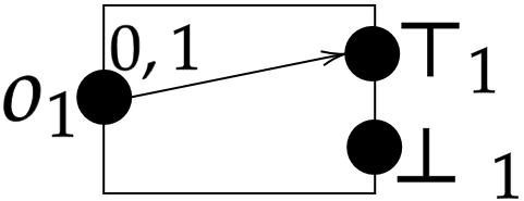
(a) $G^{1}$, the constant “true” component.

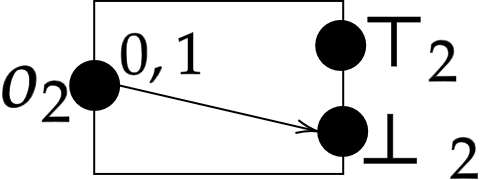
(b) $G^{2}$, the constant “false” component.

Figure 1: Initial components corresponding to constant gates “true” and “false”.

Depicted in Figure 2 are two cases corresponding to AND or OR gates. These perform a lazy evaluation of the AND or OR of components $G^{j}$ and $G^{k}$.

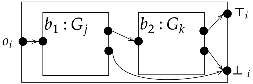
(a) Component for the AND of gates $g_{j}$ and $g_{k}$.

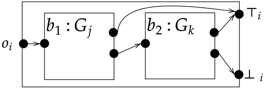
(b) Component for the OR of gates $g_{j}$ and $g_{k}$.

Figure 2: Component $G^{i}$, where $j,j^{\prime}\in[i-1]$ are the indices of the two inputs to the gate $g_{i}$. All edges correspond to both $s^{0}$ and $s^{1}$ transitions.

This process produces a polynomially sized Recursive Arrival instance for an input boolean circuit where each component $G_{j}$ can be shown inductively to reach exit $\top_{j}$ if and only if it’s corresponding gate, $g_{j}$, outputs true.

4 Recursive Arrival is in ${\mathsf{NP}}{}\cap{\mathsf{coNP}}{}$ and $\mathsf{UEOPL}$

Recall the notion of Switching Flow for an Arrival instance. For Recursive Arrival, we generalise the notion of a Switching Flow to a tuple of vectors $(\bm{x}^{1},\ldots,\bm{x}^{k})$, one for each component of the Recursive Arrival instance. We define for each component $G^{i}$, $i\in[k]$, and each box $b\in B_{i}$ the set of potential edges $F_{b,i}:=\mathsf{Call}_{b,i}\times\mathsf{Return}_{b,i}$, representing the potential ways of crossing the box $b$, assuming that the box is eventually returned from. We define the sets $F_{i}:=\cup_{b\in B_{i}}F_{b,i}$. We recall that the set of internal edges of a component $G^{i}$ is given by $E_{i}:=\{(u,v)\mid u,v\in V_{i},\ \exists\sigma\in\{0,1\},(u,\sigma,v)\in\delta_{i}\}$. We say the Flow Space for component $G^{i}$ is the set of vectors $\mathcal{F}_{i}:={{\mathbb{N}}}^{|E_{i}\cup F_{i}|}:=\{(x^{i}_{e}\in{\mathbb{N}}\mid e\in E_{i}\cup F_{i})\}$, where we identify coordinates of these vectors with edges in $E_{i}\cup F_{i}$. We define the Flow Space of $G$ to be the set $\mathcal{F}:=\Pi_{i=1}^{k}\mathcal{F}_{i}$, a tuple of $k$ vectors, with the $i$’th vector in the flow space of component $G^{i}$. We denote specifically by $\bm{0}^{i}\in\mathcal{F}_{i}$ the all zero vector, which has $\bm{0}^{i}_{e}=0$ for all $e\in E_{i}\cup F_{i}$, and $\bm{0}\in\mathcal{F}$ the all zero tuple, $\bm{0}:=(\bm{0}^{1},\ldots,\bm{0}^{k})$. We refer to elements of $\mathcal{F}$ (resp. $\mathcal{F}_{i}$) as flows on $G$ (resp. $G^{i}$).

Firstly, we define a switching flow on each component. For a Recursive Arrival instance $G:=(G^{1},\ldots,G^{k})$ and for $l\in[k]$, we call a vector $\bm{x}^{l}\in\mathcal{F}_{l}$ to be a component switching flow if the following conditions hold. Firstly, by definition, the all-zero vector $\bm{0}^{l}$ is always considered a component switching flow. Furthermore, by definition, a non-zero vector $\bm{x}^{l}\in\mathcal{F}_{l}\setminus\{\bm{0}^{l}\}$ is called a component switching flow if there exists some current-vertex $d^{l}_{\bm{x}^{l}}\in V_{l}\setminus\{o_{l}\}$ (which, as we will see, is always uniquely determined when it exists), such that for $o_{l}$ the unique entry of $G^{l}$, $\bm{x}^{l}$ satisfies the following family of conditions: $\begin{array}[]{cl}\mathrm{Flow\ Conservation}&\begin{cases}\left(\sum_{e=(u,v)\in E_{l}\cup F_{l}}x^{l}_{e}\right)&-\left(\sum_{e=(v,w)\in E_{l}\cup F_{l}}x^{l}_{e}\right)=1,\qquad\mathrm{for}\ v=d^{l}_{\bm{x}^{l}},\\ &+\left(\sum_{e=(v,w)\in E_{l}\cup F_{l}}x^{l}_{e}\right)=1,\qquad\mathrm{for}\ v=o_{l},\\ \left(\sum_{e=(u,v)\in E_{l}\cup F_{l}}x^{l}_{e}\right)&-\left(\sum_{e=(v,w)\in E_{l}\cup F_{l}}x^{l}_{e}\right)=0,\qquad\forall v\in V_{l}\setminus\{o_{l},d^{l}_{\bm{x}^{l}}\},\end{cases}\\ \\ \mathrm{Switching\ Parity\ Condition}&\;\;\;\;x_{(v,s^{1}(v))}\leq x_{(v,s^{0}(v))}\leq x_{(v,s^{1}(v))}+1,\qquad\qquad\qquad\qquad\forall v\in\mathsf{Sor}_{l},\\ \\ \mathrm{Box\ Condition}&\;\;\;\;\exists f_{b}\in F_{b,l}$ such that $\forall f\in(F_{b,l}\setminus\{f_{b}\})\ \ x^{l}_{f}=0,\qquad\qquad\forall b\in B_{l}\end{array}$

Importantly, note that for any such component switching flow, $\bm{x}^{l}$, the current-vertex node $d^{l}_{x^{l}}$ is uniquely determined. This follows from the fact that the left-hand sides of the Flow Conservation equalities for nodes $v\in V_{l}\setminus\{o_{l}\}$ are identical and independent of the specific node $v$. Hence, if a vector $\bm{x}^{l}$ satisfies all of those equalities, there can only be one vertex $v\in V_{l}\setminus\{o_{l}\}$ for which the corresponding linear expression on the left-hand side, evaluated over the coordinates of the vector $\bm{x}^{l}$, equals $1$.

In the case where $\bm{x}^{l}=\bm{0}^{l}$, i.e., the all zero-vector, we define the current-vertex of the all-zero component switching flow to be $d^{l}_{\bm{0}^{l}}:=o_{l}$. We say a component switching flow $\bm{x}^{l}\in\mathcal{F}_{l}$ is complete if its current vertex $d^{l}_{\bm{x}^{l}}$ is an exit vertex in $\mathsf{Ex}_{l}$. These conditions follow the same structure as for non-recursive switching flows, with the additional “Box Condition” only allowing at most one potential edge across each box (i.e., an edge in $F_{b,l}$) to be used.

Next, we extend our component switching flows by adding conditions that relate the flows on different components. Consider a tuple $\bm{X}:=(\bm{x}^{1},\ldots,\bm{x}^{k})\in\mathcal{F}$ of vectors, one for each component, such that each $\bm{x}^{i}\in\mathcal{F}_{i}$ is a component switching flow for component $G^{i}$. We sometimes write $d^{i}_{\bm{X}}$ instead of $d^{i}_{\bm{x}^{i}}$. Let $K_{\bm{X}}=\{i\in[k]\mid\bm{x}^{i}\ \mbox{is complete}\}$ be the subset of indices corresponding to complete component switching flows. We then say the tuple $\bm{X}\in\mathcal{F}$ is a recursive switching flow if for every $l\in[k]$, $b\in B_{l}$ and $f\in F_{b,l}$, the following holds:

• $\bm{x}^{l}\in\mathcal{F}_{l}$ is a component switching flow for component $G^{l}$, and

• if $x^{l}_{f}>0$ then $Y_{l}(b)\in K_{\bm{X}}$, and

• if $x^{l}_{f}>0$, then letting $d^{Y_{l}(b)}_{\bm{X}}\in\mathsf{Ex}_{Y_{l}(b)}$ be the current vertex of $\bm{x}^{Y_{l}(b)}$, we must have that $f=((b,o_{Y_{l}(b)}),(b,d^{Y_{l}(b)}_{\bm{X}}))$.

We define $\mathcal{R}\subset\mathcal{F}$ to be the set of all recursive switching flows. These conditions ensure “consistency” in the following way; if we use an edge $f\in F_{b,l}$ then we have a component switching flow on component $G^{Y_{l}(b)}$ which is complete and reaches the exit matching the edge $f$, and we are taking that same edge across all boxes with the same label. We note our definition implies $\bm{0}\in\mathcal{R}$, thus there is always at least one recursive switching flow. These conditions can be verified in polynomial time.

We will view recursive switching flows as hypothetical partial “runs” on each component, where an edge $e\in E_{l}\cup F_{l}$ is used $x^{l}_{e}$ times along this “run”. It may well be the case no such run actually exists. However, unlike the case of non-recursive switching flows in Arrival, it is no longer the case that any recursive switching flow where the current vertex is $d_{\bm{X}}^{1}$ in component $G^{1}$, and where $d_{\bm{X}}^{1}\in\mathsf{Ex}_{1}$ is an exit, necessarily certifies termination at $d_{\bm{X}}^{1}$. It need not do so. For example, in the instance depicted in Figure 3 we may give the following flow on $G$: $\bm{x}^{1}=(1,1,1)\ ,\ \bm{x}^{2}=(1,1,1)$. The instance depicted obviously loops infinitely, alternating calls between components $G^{1}$ and $G^{2}$, but neither ever reaching an exit. However, the given $(\bm{x}^{1},\bm{x}^{2})$ corresponds to a recursive switching flow for this instance, both of whose component switching flows have an exit as their current vertex.

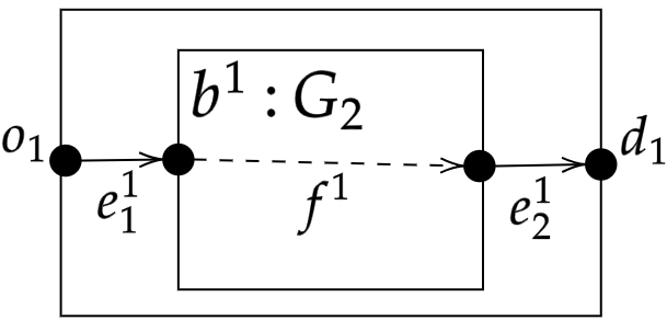
(a) Initial component $G^{1}$.

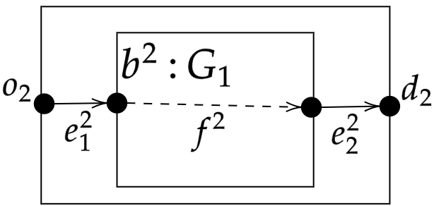
(b) Component $G^{2}$.

Figure 3: A Recursive Arrival instance $G$ on which there exists a recursive switching flow $(\bm{x}^{1},\bm{x}^{2})$ on $G$ whose current vertex is in $G^{1}$ is $d_{1}$ however the run on $G$ does not terminate, or even hit the exit $d_{1}$.

We need a way to determine whether the recursive switching flow avoids such pathologies. To do this, we need some additional definitions. We describe a component switch flow $\bm{x}^{l}$ as call-pending if its current vertex $d^{l}_{\bm{x}^{l}}\in\mathsf{Call}_{l}$ is a call port, we let $J_{\bm{X}}\subseteq[k]$ be the set of all call-pending components and we let $r_{\bm{X}}:=\lvert J\rvert$. From a recursive switching flow $\bm{X}:=(\bm{x}^{1},\ldots,\bm{x}^{k})$ we can compute the pending-call graph $C^{\mathrm{Pen}}_{\bm{X}}:=([k],E^{\mathrm{Pen}}_{\bm{X}})$ where we have edge $(i,j)\in E^{\mathrm{Pen}}_{\bm{X}}$ if and only if $i\in J_{\bm{X}}$, $d_{\bm{X}}^{i}=(b,o)\in\mathsf{Call}_{i}$ is the current vertex of $\bm{x}^{i}$ and $j=Y_{i}(b)$. We can also compute the completed-call graph, $C^{\mathrm{Com}}_{\bm{X}}:=([k],E^{\mathrm{Com}}_{\bm{X}})$, where we have an edge $(i,j)\in E^{\mathrm{Com}}_{\bm{X}}$ if and only if $\exists b\in B_{i},\ \exists f\in F_{i,b}$ with $x_{f}^{i}>0$ and $Y_{i}(b)=j$. The pending-call graph represents, from the perspective of an imagined “run” corresponding to the recursive switching flow $\bm{X}$, which components $G^{i}$ are currently “paused” at a call port and waiting for component $G^{j}$ to reach an exit to determine the return port they should move to next. The completed-call graph represents the dependencies in the calls already made in such an imagined run, where an edge from component $G^{i}$ to component $G^{j}$ means that inside component $G^{i}$ the imagined run is making a call to a box labelled by $G^{j}$ and “using” the fact that component $G^{j}$, once called upon, reaches a specific exit. In turn, in order to $G^{j}$ to reach its exit the imagined run might be “using” the completion of other components to which there are outgoing edges from $G^{j}$ in the completed-call graph. Thus, any cycle in the completed-call graph represents a series of circular (and hence not well-founded) assumptions about the imagined “run” corresponding to the recursive switching flow $\bm{X}$. For example, in the case of a 2-cycle between components $G^{i}$ and $G^{j}$, these are: “If $G^{i}$ reaches exit $d_{\bm{X}}^{i}$ then $G^{j}$ reaches exit $d_{\bm{X}}^{j}$”; and “If $G^{j}$ reaches exit $d_{\bm{X}}^{j}$ then $G^{i}$ reaches exit $d_{\bm{X}}^{i}$” (c.f. Figure 3).

Let $G$ be an instance of recursive arrival and let $\mathsf{RUN}^{\infty}(G,o_{1},q^{0}_{1}):=(\beta_{t},(v_{t},q_{t}))_{t=0}^{\infty}$ be the run starting at $(o_{1},q^{0}_{1})$. We define the times $S_{l}:=\inf\{t\mid v_{t}=o_{l}\}$ and $T_{l}:=\inf\{t\mid v_{t}\in\mathsf{Ex}_{l}\}$ for each component index $l\in[k]$, with these values being $\infty$ if the set is empty. If $S_{l}<\infty$ we define the stack $\beta^{l}:=\beta_{S_{l}}$. We define the component run to be the (potentially finite) subsequence $t_{1}^{l},t_{2}^{l},\ldots$ of times which are precisely all times $t^{l}_{j}\in[S_{l},\ldots,T_{l}]$ where $\beta_{t_{l}^{j}}=\beta^{l}$. We define the Recursive Run Profile of $G$ up to time $t$ as the sequence of vectors, $\bm{Run}(G,t):=(\bm{run}(G^{1},t),\ldots,\bm{run}(G^{k},t))$, where for each $l\in[k]$, $\bm{run}(G^{l},t):=(\lvert\{j\in{\mathbb{N}}\mid t^{l}_{j+1}\leq t\wedge(v_{t^{l}_{j}},v_{t^{l}_{j+1}})=e\}\rvert\ \mid\ e\in E_{l}\cup F_{l})$.

In other words, $\bm{run}(G^{l},t)$ is a vector that provides counts of how many times each edge in component $G^{l}$ has been crossed, up to time $t$, during one “visit” to component $G^{l}$, with some particular call stack. (The specific call stack doesn’t matter. This sequence does not depend on the specific calling context $\beta_{l}$ in which $G^{l}$ was initially called.) We note that $\bm{run}(G^{l},0)=\bm{0}^{l}$.

Similarly to the non-recursive case, we can define the last-used-edge graph for each component $G^{l}$ as, $G_{l,\bm{x}^{l}}^{*}:=(V_{l},E_{l,\bm{x}^{l}}^{*})$ who’s edge set is defined as:

$$E_{l,\bm{x}^{l}}^{*}:= \{(v,s^{0}(v))\mid v\in\mathsf{Sor}_{l}\text{ and }x^{l}_{(v,s^{0}(v))}\neq x^{l}_{(v,s^{1}(v))}\}\cup$$

$$\{(v,s^{1}(v))\mid v\in\mathsf{Sor}_{l}\text{ and }x^{l}_{(v,s^{0}(v))}=x^{l}_{(v,s^{1}(v))}>0\}\ \cup\ \{f\in F_{l}\mid x^{l}_{f}>0\}$$

We note that for the all-zero vector we have $E_{l,\bm{0}^{l}}^{*}=\emptyset$, and if $\bm{x}^{l}\neq\bm{0}^{l}$ is non-zero then the current vertex $d_{\bm{x}^{l}}^{l}$ must have at least one incoming edge in $E_{l,\bm{x}^{l}}^{*}$, and thus the set $E_{l,\bm{x}^{l}}^{*}$ isn’t empty.

Depending on how our run evolves, there are three possible cases:

• For all $l\in[k]$, if $S_{l}<\infty$ then $T_{l}<\infty$. This case corresponds to reaching some exit of $G^{1}$, i.e., terminating there.

• There exists some $l\in[k]$ with $S_{l}<\infty$ and yet with $T_{l}=\infty$, however, where for all such $l\in[k]$ the subsequence $t^{l}_{1},t^{l}_{2},\ldots$ is of finite length. This case corresponds to blowing up the call stack to arbitrarily large sizes, and as we shall describe, we can detect it by looking for a cycle in $C^{\mathrm{Pen}}_{\bm{X}}$.

• There exists $l\in[k]$ with $S_{l}<\infty$ and $T_{l}=\infty$, where the subsequence $t^{l}_{1},t^{l}_{2},\ldots$ is of infinite length. This case corresponds to getting stuck inside component $G^{l}$, and infinitely often revisiting a vertex in a loop with the same call stack. As we shall see, we can detect this case by looking for a sufficiently large entry in some coordinate of $\bm{x}^{l}$.

Let $G$ be a Recursive Arrival instance and let $\bm{X}:=(\bm{x}^{1},\ldots,\bm{x}^{k})\in\mathcal{R}$ be a recursive switching flow on $G$, we say $\bm{X}$ is run-like if it satisfies the following conditions:

• For each component index $l\in[k]$ one of the following two conditions hold:

  • The graph $G_{l,\bm{x}^{l}}^{*}$ is acyclic,

  • The graph $G_{l,\bm{x}^{l}}^{*}$ contains exactly one cycle and $d^{l}_{\bm{x}^{l}}$ is on this cycle.

• If the set of call-pending component indexes $J_{\bm{X}}$ is non-empty, then $1\in J_{\bm{X}}$ and there is some total ordering $j_{1},\ldots,j_{r_{\bm{X}}}$ of the set $J_{\bm{X}}$, with $j_{1}=1$, and a unique $j_{(r_{\bm{X}}+1)}\in[k]$ such that the edges of the pending-call graph are given by $E^{\mathrm{Pen}}_{\bm{X}}=\{(j_{i},j_{i+1})\mid i\in[r_{\bm{X}}]\}$. Note that we may have $j_{(r_{\bm{X}}+1)}=j_{m}$ for some $m\in\{1,\ldots,r_{\bm{X}}\}$, in which case $E^{\mathrm{Pen}}_{\bm{X}}$ forms not a directed line graph but a “lasso” meaning a directed line ending in one directed cycle. When $J_{\bm{X}}=\emptyset$ we say that $r_{\bm{x}}:=0$ and that $j_{1}:=1$, thus the sequence is defined for all $\bm{X}$.

• For any $l\in[k]$ either: $l\in J_{\bm{X}}\cup K_{\bm{X}}$, or $\bm{x}^{l}=(0,\ldots,0)$, or $l=j_{(r_{\bm{X}}+1)}$.

• The completed-call graph $C^{\mathrm{Com}}_{\bm{X}}:=([k],E^{\mathrm{Com}}_{\bm{X}})$ is acyclic.

• For any $l\in[k]$, if $\bm{x}^{l}\neq\bm{0}^{l}$, then in the graph $([k],E^{\mathrm{Pen}}_{\bm{X}}\cup E^{\mathrm{Com}}_{\bm{X}})$ we must have $1\rightarrow^{*}l$, i.e., there must be a path in this graph from component $1$ to all components $l$ for which $\bm{x}^{l}$ is non-zero.

We denote by $\mathcal{X}\subset\mathcal{R}$ the set of all run-like recursive switching flows on $G$. We note for any $G$ that we always have $\bm{0}\in\mathcal{X}$. We can show $\bm{X}\in\mathcal{F}$ is run-like if and only if $\exists t\in{\mathbb{N}}$, $\bm{X}=\bm{Run}(G,t)$.

We now introduce “unit vectors” for this space, we write $\bm{u}^{l}_{e}\in\mathcal{F}_{l}$ for the vector where $u^{l}_{e}=1$ and for all other $e^{\prime}\in E_{l}\cup F_{l}$ with $e^{\prime}\neq e$ that $u^{l}_{e}=0$. We then write $\bm{U}_{i,e}\in\mathcal{F}$ for the sequence of $k$ vectors $(\bm{0}^{1},\ldots,\bm{0}^{i-1},\bm{u}^{i}_{e},\bm{0}^{i+1},\ldots,\bm{0}^{k})$ where the $i$’th vector is $\bm{u}^{i}_{e}$ and for $i\neq j\in[k]$ that the $j$’th vector is the all-zero $\bm{0}^{j}$. We may naturally define the notion of addition on $\mathcal{F}$ and we define the notion of subtraction $\bm{X}-\bm{U}_{i,e}$ in the natural way whenever $x^{i}_{e}>0$, i.e., the result of the subtraction remains in ${\mathbb{N}}$ for every coordinate, subtraction is undefined where this isn’t the case. We write $\mathcal{U}:=\{\bm{U}_{i,e}\mid i\in[k],e\in E_{i}\cup F_{i}\}$ for the set of all unit vectors.

Given a run-like recursive switching flow, $\bm{X}:=(\bm{x}^{1},\ldots,\bm{x}^{k})\in\mathcal{X}$, we say that $\bm{X}$ is complete if it is the case that $1\in K_{\bm{X}}$, i.e., the current vertex $d^{1}_{\bm{x}^{1}}$ of $\bm{x}^{1}$ is an exit of $G^{1}$. We say $\bm{X}$ is lassoed when $E^{\mathrm{Pen}}_{\bm{X}}$ forms a “lasso”, meaning a directed line ending in one directed cycle, as described earlier. We note that being complete and lassoed are mutually exclusive, because either $1\in K_{\bm{X}}$ or $1\in J_{\bm{X}}$, but not both.

Lemma 4.1.

Let $G$ be an instance of Recursive Arrival, and let $\bm{X}\in\mathcal{X}$ be a run-like recursive switching flow on $G$. Then if $\bm{X}$ is neither complete nor lassoed, then there exists exactly one $\bm{U}_{i,e}\in\mathcal{U}$ such that $(\bm{X}+\bm{U}_{i,e})$ is a run-like recursive switching flow. Otherwise, if $\bm{X}$ is either complete or lassoed, then there exists no such $\bm{U}_{i,e}$.

Proof 4.2 (Proof (Sketch)).

We shall show that for any $\bm{X}$ which is neither complete nor lassoed, we are able to give unique $i$ and $e$ as a function of $\bm{X}$. Viewing $\bm{X}$ as a “hypothetical run” to some time we use $J_{\bm{X}}$ as our “call stack” at this time and use that to determine the edge to increment.

1. If $d_{\bm{X}}^{j_{(r_{\bm{X}}+1)}}\in\mathsf{Sor}_{j_{(r_{\bm{X}}+1)}}$, then the “current component” is at a switching node and we take the edge given by our switching order. We note that this includes the case where $d_{\bm{X}}^{j_{(r_{\bm{X}}+1)}}=o_{j_{(r_{\bm{X}}+1)}}$, i.e. there is a call pending to a new component.

2. If $j_{(r_{\bm{X}}+1)}\in K_{\bm{X}}$, then we can resolve the pending call in component $j_{r_{\bm{X}}}$ and increment the summary edge in $F_{j_{r_{\bm{X}}}}$ corresponding to exit $d_{\bm{X}}^{(j_{\bm{X}}+1)}$.

We can show that this is the unique choice in these cases through elimination, making use of the definitions of component, recursive, and run-like switching flows.

We define the completed call count as the function $CC:\mathcal{F}\times[k]\to{\mathbb{N}}$ which counts how many times a given component has been crossed in a given flow, defined for $\bm{X}\in\mathcal{F}$ and $l\in[k]$ as follows:

$$CC(\bm{X},l):=\sum_{i\in[k]}\quad\sum_{\{b\in B_{i}\mid Y_{i}(b)=l\}}\quad\sum_{f\in F_{b,i}}x^{i}_{f}$$

Lemma 4.3.

Let $G$ be an instance of Recursive Arrival, and let $\bm{X}\in\mathcal{X}$ be a run-like recursive switching flow on $G$. If $\bm{X}$ is non-zero then there exists a unique $\bm{U}_{i,e}\in\mathcal{U}$ such that $(\bm{X}-\bm{U}_{i,e})\in\mathcal{X}$ is a run-like recursive switching flow. Otherwise, if $\bm{X}$ is all-zero, then no such $\bm{U}_{i,e}$ exists.

Proof 4.4 (Proof (Sketch)).

We shall show for non-zero $\bm{X}$ the following choice is the unique value for $i$, and then $e$ can be determined using the last-used-edge graph in component $i$, as is the case for non-recursive switching flows. Viewing $\bm{X}$ as a “hypothetical run” to some time we use $J_{\bm{X}}$ as our “call stack” at this time and use that to determine the edge to decrement.

• If $\bm{x}^{j_{(r_{\bm{X}}+1)}}>\bm{0}^{j_{(r_{\bm{X}}+1)}}$ and $CC(\bm{X},j_{(r_{\bm{X}}+1)})=0$ then we decrement inside the “current component” as the pending-call in component $j_{r_{\bm{X}}}$ is the only call made.

• Otherwise, we take $i=j_{r_{\bm{X}}}$. Where, since we have either $CC(\bm{X},j_{(r_{\bm{X}}+1)})\geq 1$ or $\bm{x}^{j_{(r_{\bm{X}}+1)}}=\bm{0}^{j_{(r_{\bm{X}}+1)}}$ the current call from $j_{r_{\bm{X}}}$ to $j_{(r_{\bm{X}}+1)}$ is either made elsewhere and thus we cannot alter the component flow in $j_{(r_{\bm{X}}+1)}$ without affecting the edge traversed on these other calls or the flow in $j_{(r_{\bm{X}}+1)}$ is zero, in which case we step back from the final pending-call to it.

This can be shown to be the unique choice in each case through elimination.

We define the function $Val:\mathcal{F}\to{\mathbb{N}}$ as: $Val((\bm{x}^{1},\ldots,\bm{x}^{k})):=\sum_{i\in[k]}\sum_{e\in E_{i}\cup F_{i}}x^{i}_{e}$. This function sums all values across all vectors of the tuple. We note that for any flow $\bm{X}\in\mathcal{F}$ and any $i\in[k]$ and $e\in E_{i}\cup F_{i}$ that we have $Val(\bm{X}+\bm{U}_{i,e})=Val(\bm{X})+1$ and that when defined (i.e. $x^{i}_{e}>0$) that $Val(\bm{X}-\bm{U}_{i,e})=Val(\bm{X})-1$.

Recall Proposition 2.3 regarding non-recursive Arrival switching graphs, and in particular the fixed polynomial $\mathrm{p}$ which that proposition asserts the existence of. We say a recursive switching flow $\bm{X}:=(\bm{x}^{1},\ldots,\bm{x}^{k})\in\mathcal{X}$ is finished if it satisfies one of the following conditions:

1. $\bm{X}$ is complete, i.e, $1\in K_{\bm{X}}$, or, the current vertex $d_{\bm{X}}^{1}$ of $\bm{x}^{1}$ is an exit in $\mathsf{Ex}_{1}$.

2. $\bm{X}$ is lassoed, i.e., $1\not\in K_{\bm{X}}$ and $j_{(r_{\bm{X}}+1)}\in J_{\bm{X}}$, or, the edges of $E^{\mathrm{Pen}}_{\bm{X}}$ form a lasso.

3. $\bm{X}$ is just-overflowing, which we define as follows: $1\not\in K_{\bm{X}}$, and there exists some unique $l\in[k]$, and unique $e=(u,d_{\bm{X}}^{l})\in E_{l}\cup F_{l}$ with $x^{l}_{e}=2^{\mathrm{p}(\lvert V_{l}\rvert)}+1$, i.e., there is some unique component, $l$, and edge, $e$, incoming to its current vertex, $d^{l}_{\bm{X}}$, with a “just-excessively large” value in the flow $\bm{X}$.

We say the flow is post-overflowing if $1\not\in K_{\bm{X}}$, and there exists some $l\in[k]$, with $d_{\bm{X}}^{l}$ the current-vertex of $\bm{x}^{l}$, and some $e=(u,v)\in E_{l}\cup F_{l}$ satisfying at least one of: A) $x^{l}_{e}=2^{\mathrm{p}(\lvert V_{l}\rvert)}+1$ and $v\neq d_{\bm{X}}^{l}$; B) $x^{l}_{e}>2^{\mathrm{p}(\lvert V_{l}\rvert)}+1$. We note that by repeatedly applying Lemma 4.3 to a post-overflowing run-like recursive switching flow we must eventually find some finished just-overflowing run-like recursive switching flow.

We introduce the notation $\mathcal{F}^{N}\subseteq\mathcal{F}$ to be the restriction to tuples in which in every vector each coordinate is less than or equal to some $N\in{\mathbb{N}}$. Thus $\mathcal{F}^{N}$ is finite, and any element $\bm{X}\in\mathcal{F}^{N}$ can be represented using at most $(\sum_{i=1}^{k}\lvert E_{i}\cup F_{i}\rvert)\cdot\log_{2}(N)$ bits. For all our subsequent results taking $N:=2^{\mathrm{p}(\max_{l}\lvert V_{l}\rvert)}+1$ will be sufficient, noting this means elements of $\mathcal{F}^{N}$ are represented using a polynomial number of bits in our input size.

Theorem 4.5.

The Recursive Arrival problem is in ${\mathsf{NP}}{}\cap{\mathsf{coNP}}{}$ and ${\mathsf{UP}}{}\cap{\mathsf{coUP}}{}$.

Proof 4.6 (Proof (Sketch)).

The proof follows from a series of lemmas given in the full version. These show:

• For any instance of Recursive Arrival, $G$, there is a (unique) $\bm{X}\in\mathcal{F}^{N}$ which is a finished run-like recursive switching flow;

• Given any $\bm{X}\in\mathcal{F}^{N}$ we can verify whether or not $\bm{X}$ is a finished run-like recursive switching flow in $\mathsf{P}$-time;

• Given any $\bm{X}\in\mathcal{F}^{N}$ which is a finished run-like recursive switching flow, we can determine whether or not $G$ terminates and if it does terminate at which exit in $\mathsf{Ex}_{1}$ it does so.

4.1 Containment in $\mathsf{UEOPL}$

Given the previous results, we may consider a search version of Recursive Arrival as follows:

&A Recursive Arrival graph $(G^{1},\ldots,G^{k})$ Proble’missing:Compute the unique finished run-like recursive switching flow $(\bm{x}^{1},\ldots,\bm{x}^{k})\in\mathcal{F}$ on $G$ In the appendix, we show that this problem is total and hence lies in ${\mathsf{TFNP}}{}$. We show containment in the total search complexity class ${\mathsf{UEOPL}}{}$ defined by Fearnley et al. [13], as problems polynomial time many-one search reducible to UniqueEOPL, which is defined as follows:

&Given boolean circuits $S,P:\{0,1\}^{n}\to\{0,1\}^{n}$ such that $P(0^{n})=0^{n}\neq S(0^{n})$ and a boolean circuit $V:\{0,1\}^{n}\to\{0,1,\ldots,2^{m}-1\}$ such that $V(0^{n})=0$ Proble’missing:Compute one of the following:

• A point $x\in\{0,1\}^{n}$ such that $P(S(x))\neq x$.

• A point $x\in\{0,1\}^{n}$ such that $x\neq S(x)$, $P(S(x))=x$, and $V(S(x))\leq V(x)$.

• A point $x\in\{0,1\}^{n}$ such that $S(P(x))\neq x\neq 0^{n}$.

• Two points $x,y\in\{0,1\}^{n}$, such that $x\neq y$, $x\neq S(x)$, $y\neq S(y)$, and either $V(x)=V(y)$ or $V(x)<V(y)<V(S(x))$.

We may interpret an instance of UniqueEOPL as describing an exponentially large directed graph in which our vertices are points $x\in\{0,1\}^{n}$ and each vertex has both in-degree and out-degree bounded by at most one. Edges are described by the circuits $S,P$, for a fixed vertex $x\in\{0,1\}^{n}$ there is an outgoing edge from $x$ to $S(x)$ if and only if $P(S(x))=x$ and an incoming edge to $x$ from $P(x)$ if and only if $S(P(x))=x$. We are given that $0^{n}$ is a point with an outgoing edge but no incoming edge or the “start of the line”. We also have an “odometer” function, $V$, which has a minimal value at $0^{n}$. We assume our graph has the set-up of a single line $0^{n},S(0^{n}),S(S(0^{n})),\ldots$ along which the function $V$ strictly increases, with some “isolated points” where $x=S(x)=P(x)$. There are four types of solutions that can be returned, representing:

• a point which is an “end of the line”, with an incoming edge but no outgoing edge.

• a violation of the assumption that valuation $V$ strictly increases along a line, since $V(x)\not<V(S(x))$.

• a violation of the assumption there is a single line, since $x$ is the start of a line, but it is not $0^{n}$, thus it starts a distinct line.

• a violation of one of the assumptions, however, in a more nuanced way. We can assume that $P(S(x))=x$ and $P(S(y))=y$, else they’d constitute a (UV1) example too, thus neither $x$ nor $y$ is isolated and both have an outgoing edge. If $x$ and $y$ were on the same line, then either $S(\ldots S(S(x)))=y$ or $S(\ldots S(y))=x$ by doing this iteration we’d eventually find some $z\in\{0,1\}^{n}$ where $V(z)\not<V(S(z))$, violating (UV1). However, if $x$ and $y$ are on different lines, then that would imply the existence of two distinct lines, violating (UV2). Thus, a (UV3) violation is a short proof of existence of a (UV1) or (UV2) violation elsewhere in the instance.

For our reduction, our space will be made up of all possible flows $(\bm{x}^{1},\ldots,\bm{x}^{k})\in\mathcal{F}^{N}$ and our line will be made up of those arising from distinct $\bm{Run}(G,t)$’s, each step increasing in $t$ until we reach a finished flow, with all other vectors being isolated. A type (U1) solution will correspond to a finished run-like recursive switching flow, and we will show our instance has no (UV1-3) solutions, thus our computed solution to UniqueEOPL will be a solution to Search Recursive Arrival.

Given any flow $\bm{X}\in\mathcal{F}$ we can verify whether or not $\bm{X}$ is a run-like recursive switching flow (i.e. $\bm{X}\in\mathcal{X}\subset\mathcal{F}$). We will use this fact in our definitions of functions $Adv:\mathcal{F}\to\mathcal{F}$ and $Prev:\mathcal{F}\to\mathcal{F}$.

Our function $Adv$ on some value $\bm{X}:=(\bm{x}^{1},\ldots,\bm{x}^{k})\in\mathcal{F}$ is defined by the following sequence:

1. If $\bm{X}\not\in\mathcal{X}$ then we take $Adv(\bm{X})=\bm{X}$.

2. Else if $\bm{X}\in\mathcal{X}$ is either finished or post-overflowing then we take $Adv(\bm{X})=\bm{X}$.

3. Otherwise, take $Adv(\bm{X})=\bm{X}+\bm{U}_{i,e}$, for the unique $\bm{U}_{i,e}\in\mathcal{U}$ such that $\bm{X}+\bm{U}_{i,e}\in\mathcal{X}$ (Lemma 4.1).

We note by this process that if $Adv(\bm{X})\neq\bm{X}$, then $Val(Adv(\bm{X}))=Val(\bm{X})+1$, since we have incremented exactly one edge in exactly one vector. Hence, this is consistent with our odometer. We may also define the operation $Prev:\mathcal{F}\to\mathcal{F}$ analogously on some value $\bm{X}:=(\bm{x}^{1},\ldots,\bm{x}^{k})\in\mathcal{F}$. Taking $Prev(\bm{X})=\bm{X}$ whenever: $\bm{X}\not\in\mathcal{X}$; $\bm{X}=\bm{0}$, or; $\bm{X}$ is post-overflowing. Otherwise, taking $Prev(\bm{X})=\bm{X}-\bm{U}_{i,e}$, for the unique $\bm{U}_{i,e}\in\mathcal{U}$ such that $\bm{X}-\bm{U}_{i,e}\in\mathcal{X}$ (Lemma 4.3). Observe that, for any non-zero $\bm{X}\in\mathcal{X}$, that $Adv(Prev(\bm{X}))=\bm{X}$, and, for any $\bm{X}\in\mathcal{X}$, if we have $Prev(Adv(\bm{X}))\neq\bm{X}$, then $\bm{X}$ must be finished.

Theorem 4.7.

The Search-Recursive Arrival is in $\mathsf{UEOPL}$.

Proof 4.8 (Proof (Sketch)).

We will give a polynomial-time search reduction from Search Recursive Arrival to the UniqueEOPL problem. We compute boolean circuits $S,P$ and $V$ which will be given by the restriction of the functions $Adv$, $Prev$, and $Val$ to the domain $\mathcal{F}^{N}$. This process involves computing membership of $\mathcal{X}$ and then computing the unique values $i$ and $e$ given by Lemmas 4.1 and 4.3 for $Adv$ and $Prev$ respectively. We can then show that the only $\mathsf{UEOPL}$ solution is of type (U1) and is a run-like recursive switching flow, which is a solution we are looking for.

5 Conclusions

We have shown that Recursive Arrival is contained in many of the same classes as the standard Arrival problem. While we have shown $\mathsf{P}$-hardness for Recursive Arrival, whether or not Arrival is $\mathsf{P}$-hard remains open.

Let us note that the way we have chosen to generalise Arrival to the recursive setting uses one of two possible natural choices for its semantics. Namely, it assumes a “local” semantics, meaning that the current switch position for each component on the call stack is maintained as part of the current state. An alternative “global” semantics would instead consider the switch position of each component as a “global variable”. In such a model all switch positions would start in an initial position, and as the run progresses the switch positions would persist between, and be updated during, different calls to the same component. It is possible to show (a result we have not included in this paper) that such a “global” formulation immediately results in $\mathsf{PSPACE}$-hardness of reachability and termination problems.

As mentioned in the introduction, a stochastic version of Arrival, in which some nodes are switching nodes whereas other nodes are chance (probabilistic) nodes with probabilities on outgoing transitions, has already been studied in [20], building on the work of [13] which generalises Arrival by allowing switching and player-controlled nodes. There is extensive prior work on RMCs and RMDPs, with many known decidability/complexity results (see, e.g., [10, 11]). It would be natural to ask similar computational questions for the generalisation of RMCs and RMDPs to a recursive Arrival model combining switching nodes with chance (probabilistic) nodes and controlled/player nodes.

Finally, we note that Fearnley et al. also defined a $\mathsf{P}$-hard generalisation of Arrival in [13] which uses “succinct switching orders” to succinctly encode an exponentially larger switch graph. We will refer to this problem as Succinct Arrival. We don’t know whether there are any P-time reduction, in either direction, between Recursive Arrival and Succinct Arrival. It has been observed that the results of [15] imply that both Arrival and Succinct Arrival are P-time reducible to the Tarski problem defined in [8]. Succinct Arrival is also contained in $\mathsf{UEOPL}$ by the same arguments as for Arrival. We do not currently know whether Recursive Arrival is P-time reducible to Tarski.

Acknowledgements. Thanks to my PhD supervisor Kousha Etessami for his support.

References

- [1]
- [2] Rajeev Alur, Kousha Etessami & Mihalis Yannakakis (2001): Analysis of Recursive State Machines. In Gérard Berry, Hubert Comon & Alain Finkel, editors: Computer Aided Verification, Springer Berlin Heidelberg, Berlin, Heidelberg, pp. 207–220, 10.5555/647770.734260.
- [3] David Auger, Pierre Coucheney & Loric Duhaze (2022): Polynomial Time Algorithm for ARRIVAL on Tree-like Multigraphs. In: International Symposium on Mathematical Foundations of Computer Science, 10.48550/arXiv.2204.13151.
- [4] Ahmed Bouajjani, Javier Esparza & Oded Maler (1997): Reachability analysis of pushdown automata: Application to model-checking. In Antoni Mazurkiewicz & Józef Winkowski, editors: CONCUR ’97: Concurrency Theory, Springer Berlin Heidelberg, Berlin, Heidelberg, pp. 135–150, 10.1007/3-540-63141-0_10.
- [5] Anne Condon (1992): The Complexity of Stochastic Games. Inf. Comput. 96(2), pp. 203–224, 10.1016/0890-5401(92)90048-K.
- [6] Jérôme Dohrau, Bernd Gärtner, Manuel Kohler, Jíri Matoušek & Emo Welzl (2017): A Journey through Discrete Mathematics: A Tribute to Jiri Matousek, chapter Arrival: A zero-player graph game in , pp. 367–374. Springer, 10.1007/978-3-319-44479-6_14.
- [7] Javier Esparza, Antonin Kucera & Richard Mayr (2006): Model Checking Probabilistic Pushdown Automata. Logical Methods in Computer Science Volume 2, Issue 1, 10.2168/LMCS-2(1:2)2006.
- [8] Kousha Etessami, Christos H. Papadimitriou, Aviad Rubinstein & Mihalis Yannakakis (2020): Tarski’s Theorem, Supermodular Games, and the Complexity of Equilibria. In Thomas Vidick, editor: 11th Innovations in Theoretical Computer Science Conference, ITCS 2020, January 12-14, 2020, Seattle, Washington, USA, LIPIcs 151, pp. 18:1–18:19, 10.4230/LIPIcs.ITCS.2020.18.
- [9] Kousha Etessami & Mihalis Yannakakis (2008): Recursive Concurrent Stochastic Games. CoRR abs/0810.3581, 10.48550/arXiv.0810.3581. arXiv:https://arxiv.org/abs/0810.3581.
- [10] Kousha Etessami & Mihalis Yannakakis (2009): Recursive Markov chains, stochastic grammars, and monotone systems of nonlinear equations. J. ACM 56(1), pp. 1:1–1:66, 10.1145/1462153.1462154.
- [11] Kousha Etessami & Mihalis Yannakakis (2015): Recursive Markov Decision Processes and Recursive Stochastic Games. J. ACM 62(2), pp. 11:1–11:69, 10.1145/2699431.
- [12] John Fearnley, Martin Gairing, Matthias Mnich & Rahul Savani (2021): Reachability Switching Games. Log. Methods Comput. Sci. 17(2), 10.23638/LMCS-17(2:10)2021.
- [13] John Fearnley, Spencer Gordon, Ruta Mehta & Rahul Savani (2019): Unique End of Potential Line. In: 46th International Colloquium on Automata, Languages, and Programming (ICALP 2019), LIPIcs 132, pp. 56:1–56:15, 10.4230/LIPIcs.ICALP.2019.56.
- [14] Bernd Gärtner, Thomas Dueholm Hansen, Pavel Hubácek, Karel Král, Hagar Mosaad & Veronika Slívová (2018): ARRIVAL: Next Stop in CLS. In: 45th International Colloquium on Automata, Languages, and Programming, LIPIcs 107, pp. 60:1–60:13, 10.4230/LIPIcs.ICALP.2018.60.
- [15] Bernd Gärtner, Sebastian Haslebacher & Hung P. Hoang (2021): A Subexponential Algorithm for ARRIVAL. In: 48th International Colloquium on Automata, Languages, and Programming, LIPIcs 198, pp. 69:1–69:14, 10.4230/LIPIcs.ICALP.2021.69.
- [16] Raymond Greenlaw, H. James Hoover & Walter L. Ruzzo (1995): Limits to Parallel Computation. Oxford University Press, 10.1093/oso/9780195085914.001.0001.
- [17] Marcin Jurdzinski (1998): Deciding the Winner in Parity Games is in . Inf. Process. Lett. 68(3), pp. 119–124, 10.1016/S0020-0190(98)00150-1.
- [18] C. S. Karthik (2017): Did the train reach its destination: The complexity of finding a witness. Information Processing Letters 121, pp. 17–21, 10.1016/j.ip1.2017.01.004.
- [19] Graham Manuell (2021): A simple lower bound for ARRIVAL. CoRR abs/2108.06273, 10.48550/arXiv.2108.06273.
- [20] Thomas Webster (2022): The Stochastic Arrival Problem. In Anthony W. Lin, Georg Zetzsche & Igor Potapov, editors: Reachability Problems, Springer, pp. 93–107, 10.1007/978-3-031-19135-0_7.
- [21] Uri Zwick & Mike Paterson (1996): The Complexity of Mean Payoff Games on Graphs. Theor. Comput. Sci. 158(1&2), pp. 343–359, 10.1016/0304-3975(95)00188-3.