Probability Conservation and Localization in a One-Dimensional Non-Hermitian System

Abstract

We consider transport through a non-Hermitian conductor connected to a pair of Hermitian leads and analyze the underlying non-Hermitian scattering problem. In a typical non-Hermitian system, such as a Hatano–Nelson-type asymmetric hopping model, the continuity of probability and probability current is broken at a local level. As a result, the notion of transmission and reflection probabilities becomes ill-defined. Instead of these probabilities, we introduce the injection rate $R_{\rm I}=1-|{\cal R}|^{2}$ and the transmission rate $R_{\rm T}=|{\cal T}|^{2}$ as relevant physical quantities, where ${\cal T}$ and ${\cal R}$ are the transmission and reflection amplitudes, respectively. In a generic non-Hermitian case, $R_{\rm I}$ and $R_{\rm T}$ have independent information. We provide a modified continuity equation in terms of incoming and outgoing currents, from which we derive a global probability conservation law that relates $R_{\rm I}$ and $R_{\rm T}$. We have tested the usefulness of our probability conservation law in the interpretation of numerical results for non-Hermitian localization and delocalization phenomena.

1 Introduction

The non-Hermitian quantum mechanics prescribed by a non-Hermitian Hamiltonian is relevant to the description of an open quantum system, i.e., a quantum system coupled to an environment. [1, 2] Historically, the idea of non-Hermitian quantum mechanics dates back to that of an optical potential [3, 4, 5] in the scattering theory for the description of nuclear decay in terms of resonant states with complex eigenvalues. In Hermitian quantum mechanics, the scattering problem is a typical setup and describes a situation in which an incident wave is scattered in various directions by a given potential. Let us consider a one-dimensional lattice system of infinite length with the lattice constant $a$ and assume that a finite region of $n\in[1,N]$ serves as a scattering region, where $n$ specifies a site on the lattice system. When a plane wave $e^{ikna}$ ($n\leq 0$) is incident in the scattering region, it is either transmitted or reflected. The corresponding wave function is given by $e^{ikna}\ +{\cal R}e^{-ikna}$ in the region of $n\leq 0$ and by ${\cal T}e^{ikna}$ in the region of $n\geq N+1$, where ${\cal T}$ and ${\cal R}$ are the transmission and reflection amplitudes, respectively. All the information of the scattering problem is encoded in these complex amplitudes. The quantities $T=|{\cal T}|^{2}$ and $R=|{\cal R}|^{2}$ satisfy the identity

$$T+R=1,$$ (1)

which is interpreted as the manifestation of probability conservation. This allows us to interpret $T$ and $R$ as the transmission and reflection probabilities, respectively. In Hermitian quantum mechanics, identity (1) always holds. However, Eq. (1) does not necessarily hold in a non-Hermitian scattering problem. [6, 7, 8, 9, 10, 11, 12, 13, 14, 15, 16, 17, 18, 19, 20, 21, 22] As a result, $T$ and $R$ cannot be regarded as probabilities. They need to be reinterpreted.

More generically, setting aside the scattering problem for the moment, the probability conservation in quantum mechanics can be expressed locally in the form of a continuity equation of probability and probability current. In a one-dimensional lattice system, this reads

$$\frac{\partial\rho_{n}(t)}{\partial t}=j_{n-\frac{1}{2}}(t)-j_{n+\frac{1}{2}}(t),$$ (2)

where the probability $\rho_{n}(t)$ of finding an electron at the $n$th site is related to the corresponding wave function $\psi_{n}(t)$ as $\rho_{n}(t)=|\psi_{n}(t)|^{2}$. [23] Note that the probability $\rho_{n}(t)$ is defined on the $n$th site, whereas the probability current $j_{n+\frac{1}{2}}(t)$ is defined on the link $(n,n+1)$. The explicit form of $j_{n+\frac{1}{2}}(t)$ is model-dependent and is determined by the quantum dynamics of the system driven by the Schrödinger equation. In the case of the simple tight-binding model

$$H_{0}=\sum_{n}\biggl{[}-\Gamma|n\rangle\langle n+1|-\Gamma|n+1\rangle\langle n|\biggr{]},$$ (3)

$j_{n+\frac{1}{2}}(t)$ reads

$$j_{n+\frac{1}{2}}(t)=i\frac{\Gamma}{\hbar}\left[\psi_{n+1}(t)^{*}\psi_{n}(t)-\psi_{n+1}(t)\psi_{n}(t)^{*}\right].$$ (4)

The continuity equation (2) assures a consistent probabilistic interpretation of quantum mechanics. In a non-Hermitian system, the continuity equation (2) does not hold as it is. [15, 10, 24, 25] Let us consider the simplest case where an imaginary scalar potential $i\gamma_{n}$ is added to Eq. (3) as

$$H_{\gamma}=\sum_{n}\biggl{[}-\Gamma|n\rangle\langle n+1|-\Gamma|n+1\rangle\langle n|+i\gamma_{n}|n\rangle\langle n|\biggr{]}.$$ (5)

In this case, the continuity equation (2) acquires a correction:

$$\frac{\partial\rho_{n}(t)}{\partial t}=j_{n-\frac{1}{2}}(t)-j_{n+\frac{1}{2}}(t)+\frac{2}{\hbar}\gamma_{n}\rho_{n}(t),$$ (6)

revealing that the probability conservation is broken in the sense of Hermitian quantum mechanics. The imaginary scalar potential $i\gamma_{n}$ serves as a local source of gain or loss of the probability. One can regard that this describes the injection or leakage of the probability current due to the coupling of the system with a reservoir. If this hypothetical reservoir is taken into consideration, one can say that the probability is still conserved. In the sense of this modified probabilistic interpretation, one can interpret the wave function $\psi_{n}(t)$ as a complex probability amplitude. However, in a more generic non-Hermitian situation, it is unclear whether such an ad hoc reinterpretation of the breaking of probability conservation is always possible. For example, in the case of the Hatano–Nelson-type tight-binding model with asymmetric hopping, [26, 27]

$$H_{\rm HN}=\sum_{n}\biggl{[}-\Gamma_{L}|n\rangle\langle n+1|-\Gamma_{R}|n+1\rangle\langle n|\biggr{]},$$ (7)

such a reinterpretation as that in the case of Eq. (6) is ineffective. [25, 28]

In this paper, we attempt to develop a more general framework to overcome the apparent breakdown of probability conservation in a non-Hermitian system. As a concrete example, we focus on the one-dimensional scattering problem in which a scattering region is described by a non-Hermitian Hamiltonian with both the asymmetric hopping and the imaginary scalar potential. For this system, we obtain a global probability conservation law that leads us to define the injection rate $R_{\rm I}=1-|{\cal R}|^{2}$ and the transmission rate $R_{\rm T}=|{\cal T}|^{2}$ as relevant physical quantities. We show that the probability conservation law is useful in interpreting numerical results for the localization and delocalization phenomena in the system.

Figure 1: Schematics of the system. (a) One-dimensional non-Hermitian model consisting of a non-Hermitian region (thick solid line) and two Hermitian leads (solid lines). (b) Hermitian system consisting of a one-dimensional system and a reservoir, which underlies the non-Hermitian model shown in panel (a). The non-Hermiticity of the model in panel (a) is assumed to arise from the coupling of the one-dimensional system with the reservoir.

2 Non-Hermitian scattering problem

We consider the following setup extended to one-dimensional lattice sites $n=0,\pm 1,\pm 2,\cdots$ in which a non-Hermitian scattering region $n\in[1,N]$ prescribed by a non-Hermitian Hamiltonian $H_{\rm S}$ is connected to two semi-infinite Hermitian leads. The left lead extended to $n\rightarrow-\infty$ is described by $H_{\rm L}$, and the right lead extended to $n\rightarrow\infty$ is described by $H_{\rm R}$. The total Hamiltonian is given by $H=H_{\rm L}+H_{\rm S}+H_{\rm R}$, where

$$H_{\rm L} =\sum_{n\leq 0}\biggl{[}-\Gamma|n\rangle\langle n+1|-\Gamma|n+1\rangle\langle n|\biggr{]},$$ (8)

$$H_{\rm S} =\sum_{1\leq n\leq N-1}\biggl{[}-\Gamma_{\rm L}|n\rangle\langle n+1|-\Gamma_{\rm R}|n+1\rangle\langle n|\biggr{]}$$

$$\hskip 28.45274pt+\sum_{1\leq n\leq N}\left(V_{n}+i\gamma_{n}\right)|n\rangle\langle n|,$$ (9)

$$H_{\rm R} =\sum_{n\geq N}\biggl{[}-\Gamma|n\rangle\langle n+1|-\Gamma|n+1\rangle\langle n|\biggr{]},$$ (10)

where $\Gamma$, $\Gamma_{\rm L}$, and $\Gamma_{\rm R}$ as well as $V_{n}$ and $\gamma_{n}$ with $n\in[1,N]$ are chosen to be real. Note that $H_{\rm S}$ contains two sources of non-Hermiticity:

• the imaginary scaler potential $i\gamma_{n}$ representing gain or loss,

• the asymmetric hopping $\Gamma_{\rm L}\neq\Gamma_{\rm R}$,

and the random scattering potential $V_{n}$ as well. The advantage of this setup is that we can set the energy of a stationary scattering state to be a real value. Let us assume that a plane wave $\psi_{n}^{\rm(in)}=e^{ikna}$ ($n\leq 0$) specified by a real wavenumber $k$ is incident in the non-Hermitian scattering region $n\in[1,N]$ from the left lead. Inside the left lead, its energy is fixed to be a real value of $E=-2\Gamma\cos(ka)$; hence, the energy of the resulting stationary scattering state $|\psi\rangle$ must also have the same real energy everywhere in the system. The stationary scattering state

$$|\psi(t)\rangle=e^{-i\frac{Et}{\hbar}}\sum_{n}\psi_{n}|n\rangle,$$ (11)

with

$$\psi_{n}=e^{ikna}+{\cal R}e^{-ikna}$$ (12)

for $n\leq 0$ and

$$\psi_{n}={\cal T}e^{ikna}$$ (13)

for $n\geq N+1$ satisfies the time-dependent Schrödinger equation

$$i\hbar\frac{\partial}{\partial t}|\psi(t)\rangle=H|\psi(t)\rangle,$$ (14)

where the total Hamiltonian $H$ is composed of the three parts given in Eqs. (8)–(10).

The two panels in Fig. 1 illustrate our setup consisting of a non-Hermitian conductor connected to two Hermitian leads. The central scattering region is described by an effective non-Hermitian Hamiltonian [see panel (a)]. We assume that its non-Hermiticity arises from the coupling of an underlying Hermitian system to an external reservoir [see panel (b)]. However, we do not attempt to derive the effective Hamiltonian (9) from a microscopic Hermitian model. [29, 30, 31]

As for alternative realizations of a Hatano–Nelson-type asymmetric hopping model, we refer the readers to recent experiments, [32, 33, 34, 35] in which the so-called non-Hermitian skin effect characteristic of such an asymmetric hopping model under the open boundary condition has been demonstrated.

Figure 2: Schematic representation of probability current. (a) $j_{n}^{\rm(in)}$ and $j_{n}^{\rm(out)}$ are defined for the $n$th site. (b) $j_{n+1}^{\rm(in)}=\frac{\Gamma_{\rm R}}{\Gamma_{\rm L}}j_{n}^{\rm(out)}$ means that the coupling with the reservoir amplifies (attenuates) a right-going (left-going) wave when $\frac{\Gamma_{\rm R}}{\Gamma_{\rm L}}>1$.

3 Incoming and outgoing currents

We have pointed out that in the non-Hermitian scattering region $n\in[1,N]$ prescribed by Eq. (9), the continuity equation (6), associated with the standard Hermitian current $j_{n+\frac{1}{2}}$ given in Eq. (4), is no longer valid. Yet, we have also noted that the definition of current that appears in the continuity equation is generally model-dependent. If so, can we think of an alternative definition of current that makes the continuity equation valid in the non-Hermitian scattering region?

To find such an expression of current, we consider the time evolution of an arbitrary state,

$$|\psi(t)\rangle=\sum_{n}\psi_{n}(t)|n\rangle,$$ (15)

driven by the Schrödinger equation (14). Its Hermitian conjugate $\langle\psi(t)|=|\psi(t)\rangle^{\dagger}$ obeys

$$-i\hbar\frac{\partial}{\partial t}\langle\psi(t)|=\langle\psi(t)|H^{\dagger},$$ (16)

where $H$ is generically non-Hermitian (i.e., $H\neq H^{\dagger}$). By considering the time evolution of the probability,

$$\rho_{n}(t)=\langle\psi(t)|n\rangle\langle n|\psi(t)\rangle,$$ (17)

one finds that the modified continuity equation

$$\frac{\partial}{\partial t}\rho_{n}(t)=j_{n}^{\rm(in)}(t)-j_{n}^{\rm(out)}(t)+\frac{2\gamma_{n}}{\hbar}\rho_{n}(t)$$ (18)

holds in the scattering region if one introduces the incoming current $j_{n}^{\rm(in)}(t)$ and the outgoing current $j_{n}^{\rm(out)}(t)$ defined as

$$j_{n}^{\rm(in)}(t) =i\frac{\Gamma_{\rm R}}{\hbar}\left[\psi_{n}(t)^{*}\psi_{n-1}(t)-\psi_{n}(t)\psi_{n-1}(t)^{*}\right],$$ (19)

$$j_{n}^{\rm(out)}(t) =i\frac{\Gamma_{\rm L}}{\hbar}\left[\psi_{n+1}(t)^{*}\psi_{n}(t)-\psi_{n+1}(t)\psi_{n}(t)^{*}\right].$$ (20)

As shown in Fig. 2(a), the two probability currents $j_{n}^{\rm(out)}(t)$ and $j_{n+1}^{\rm(in)}(t)$ are associated with the same link $(n,n+1)$. They differ from each other when $\Gamma_{\rm L}\neq\Gamma_{\rm R}$ and are necessary to describe local probability conservation in the presence of asymmetric hopping.

In the Hermitian region consisting of the left and right leads, the incoming current Eq. (19) and the outgoing current Eq. (20) reduce to the Hermitian current (4). That is, both $j_{n}^{\rm(out)}(t)$ and $j_{n+1}^{\rm(in)}(t)$ reduce to $j_{n+\frac{1}{2}}(t)$ for $n\leq 0$ and for $n\geq N$.

4 Local and global probability conservation

Let us consider a more specific situation in which $|\psi(t)\rangle$ given in Eq. (15) is replaced with a stationary scattering state specified by Eq. (11) with real energy. In this case, $\rho_{n}$, $j_{n}^{\rm(in)}$, and $j_{n}^{\rm(out)}$ do not depend on time and Eq. (18) yields

$$j_{n}^{\rm(out)}=j_{n}^{\rm(in)}+\frac{2\gamma_{n}}{\hbar}\rho_{n}.$$ (21)

Note that $j_{n}^{\rm(out)}$ flowing out of the $n$th site is different from $j_{n}^{\rm(in)}$ flowing into the same site. The difference is given by the second term on the right-hand side of Eq. (21) and interpreted as the injection or leakage (depending on the sign of $\gamma_{n}$) of the probability current [see Fig. 2(b)] due to the imaginary potential in Eq. (9). Recall our assumption that this term stems from the coupling of the system with a reservoir that has been traced out when deriving the effective Hamiltonian (9). The imaginary potential $i\gamma_{n}$ contributes additively to the probability current [see Eqs. (21) and (23)].

Let us also focus on $j_{n}^{\rm(out)}$ and $j_{n+1}^{\rm(in)}$, both of which are associated with the same link $(n,n+1)$ [see Fig. 2(a)]. Comparing the definitions of the incoming and outgoing currents given in Eqs. (19) and (20), respectively, one immediately finds

$$j_{n+1}^{\rm(in)}=\frac{\Gamma_{\rm R}}{\Gamma_{\rm L}}j_{n}^{\rm(out)}.$$ (22)

This makes the role of asymmetry between $\Gamma_{\rm L}$ and $\Gamma_{\rm R}$ apparent. On a given link $(n,n+1)$, $j_{n}^{\rm(out)}$ flowing out of the $n$th site is augmented by the factor $\Gamma_{\rm R}/\Gamma_{\rm L}$ when it gets out of the link and becomes $j_{n+1}^{\rm(in)}$ flowing into the neighboring $n+1$th site. In other words, there has been again an inflow or leakage (depending on the direction of asymmetry) of current on the link [see Fig. 2(b)]. Similarly to the case of the imaginary potential $i\gamma_{n}$, we can interpret that this amplification or attenuation of the probability current stems from the coupling of the system with the reservoir. Note also that the asymmetric hopping modifies the probability current in a multiplicative manner.

To summarize, Eqs. (21) and (22) constitute the local conservation law of probability valid in the non-Hermitian scattering region prescribed by Eq. (9), in which the continuity of the probability current in the Hermitian sense [see Eq. (2)] is no longer applicable.

Using Eqs. (21) and (22) iteratively, one finds

$$j_{N}^{\rm(out)}=\left(\frac{\Gamma_{\rm R}}{\Gamma_{\rm L}}\right)^{N-1}j_{1}^{\rm(in)}+\sum_{n=1}^{N}\left(\frac{\Gamma_{\rm R}}{\Gamma_{\rm L}}\right)^{N-n}\frac{2\gamma_{n}}{\hbar}\rho_{n}.$$ (23)

If one recalls that the probability current is conserved in the left and right Hermitian leads, i.e.,

$$j_{1}^{\rm(in)} =j_{0}^{\rm(out)}=j_{0}^{\rm(in)}=j_{-1}^{\rm(out)}=\cdots\equiv j_{\rm L},$$ (24)

$$j_{N}^{\rm(out)} =j_{N+1}^{\rm(in)}=j_{N+1}^{\rm(out)}=j_{N+2}^{\rm(in)}=\cdots\equiv j_{\rm R}$$ (25)

with

$$j_{\rm L} =\frac{2\Gamma\sin(ka)}{\hbar}(1-|{\cal R}|^{2}),$$ (26)

$$j_{\rm R} =\frac{2\Gamma\sin(ka)}{\hbar}|{\cal T}|^{2},$$ (27)

and substitutes Eqs. (24)–(27) into Eq. (23), one can rewrite Eq. (23) as

$$|{\cal T}|^{2} =\left(\frac{\Gamma_{\rm R}}{\Gamma_{\rm L}}\right)^{N-1}(1-|{\cal R}|^{2})$$

$$+\sum_{n=1}^{N}\left(\frac{\Gamma_{\rm R}}{\Gamma_{\rm L}}\right)^{N-n}\frac{\gamma_{n}\rho_{n}}{\Gamma\sin(ka)},$$ (28)

which serves as a global conservation law of probability. Note that Eq. (4) still holds in the presence of the disorder potential $V_{n}$.

In the Hermitian limit of $\Gamma_{\rm R}/\Gamma_{\rm L}=1$ and $\gamma_{n}=0$, Eq. (4) reduces to Eq. (1) with

$$0\leq|{\cal T}|^{2}\leq 1,\hskip 14.22636pt0\leq|{\cal R}|^{2}\leq 1.$$ (29)

In the non-Hermitian case of $\Gamma_{\rm R}/\Gamma_{\rm L}\neq 1$ and/or $\gamma_{n}\neq 0$, $|{\cal T}|^{2}\geq 0$ and $|{\cal R}|^{2}\geq 0$ still hold, whereas both of $|{\cal T}|^{2}$ and $|{\cal R}|^{2}$ can be larger than $1$. That is, Eq. (1) no longer holds. The case of $|{\cal R}|^{2}>1$ may be rare but is possible; preliminary numerical calculations show that this is indeed the case (see the first paragraph of Sect. 5). In contrast, the case of $|{\cal T}|^{2}>1$ is typical as a result of the amplification effect due to $\Gamma_{\rm R}/\Gamma_{\rm L}>1$ as well as $\gamma>0$. Indeed, it is likely that the transmission probability exceeds $1$. [11, 22] Again, under such circumstances, one can presume that an effective current is injected from the hypothetical reservoir that has been traced out in the process of deriving the effective Hamiltonian (9).

The invalidity of the global probability conservation law (1) in the generic non-Hermitian case suggested by Eq. (4) implies that the interpretation of the quantities $T=|{\cal T}|^{2}$ and $R=|{\cal R}|^{2}$ as the transmission and reflection probabilities, respectively, is no longer appropriate. In the Hermitian case, the Landauer formula [36, 37] relates the two-terminal conductance $G_{2}$ of a mesoscopic conductor to the transmission probability $T=|{\cal T}|^{2}$ as $G_{2}=(e^{2}/h)T$. To be precise, zero temperature is assumed and $T$ should be evaluated at the Fermi energy. For a bias voltage $V$ applied between the left and right leads, an influx $I_{L}^{+}=(e^{2}/h)V$ of electrons is injected from the left lead, whereas the outflux to the right lead is $I_{R}^{+}=T(e^{2}/h)V$. The remaining flux, $I_{L}^{-}=R(e^{2}/h)V$, is reflected back to the left lead, where $R=1-T$ is the probability that an electron injected from the left lead is reflected back to the same lead. These ensure that the net current $I$,

$$I=I_{L}^{+}-I_{L}^{-}=I_{R}^{+}=T(e^{2}/h)V,$$ (30)

is conserved throughout in the system. The two-terminal Landauer formula [36] describes such a situation. In the non-Hermitian case of invalidated probability conservation with typically $T>1$ and possibly $R>1$, the central identity of Eq. (30) fails and Eq. (1) should be replaced with Eq. (4).

The net currents $I_{L}=I_{L}^{+}-I_{L}^{-}$ on the left incident side and $I_{R}=I_{R}^{+}$ on the right transmitted side differ and have independent information. In this case, one should deal with $I_{L}$ and $I_{R}$ independently by introducing the following two quantities:

$$I_{L}/I_{L}^{+} =1-R\equiv R_{\rm I},$$ (31)

$$I_{R}/I_{L}^{+} =T\equiv R_{\rm T}.$$ (32)

Keeping in mind that $T$ and $R$ should no longer be called probabilities, let us call $R_{\rm I}$ and $R_{\rm T}$ the injection and transmission rates, respectively.

The fact that $I_{L}\neq I_{R}$ in the generic non-Hermitian case is also consistent with our previous assumption that an effective current is either injected from or leaked to a hypothetical reservoir in the non-Hermitian scattering region. Such a hypothetical reservoir is assumed to be connected to the scattering region in the underlying Hermitian model. In this sense, the non-Hermitian setup considered in this work is certainly beyond the description based on the two-terminal Landauer conductance $G_{2}$.

5 Numerical tests

Let us consider the injection and transmission rates introduced in Eqs. (31) and (32), respectively. In the Hermitian limit, they reduce to $R_{\rm I}=R_{\rm T}=T$. They obviously satisfy $R_{\rm I}\leq 1$ and $R_{\rm T}\geq 0$. However, $R_{\rm I}\geq 0$ and $R_{\rm T}\leq 1$ are not guaranteed. Indeed, preliminary numerical calculations show that $R_{\rm I}$ can become negative when $\gamma>0$. Here and hereafter, we assume for simplicity that the imaginary potential $i\gamma_{n}$ is uniform in the scattering region of $n\in[1,N]$ as

$$i\gamma_{n}=i\gamma.$$ (33)

The situation $R_{\rm I}<0$ is induced by injection from the hypothetical reservoir near the left end of the scattering region when a large portion of this injection is converted into the left-going current by a strong disorder such that $R=1-R_{\rm I}>1$. We leave this situation for a future study and restrict our consideration to the case of $\gamma\leq 0$, in which $0\leq R_{\rm I}\leq 1$. Once $0\leq R_{\rm I}\leq 1$ is ensured, we accept the situation $R_{\rm T}>1$ as a result of the amplification due to the non-Hermiticity describing the coupling with the reservoir.

Let us now examine the localization and delocalization phenomena in the non-Hermitian disordered system. [26, 27] The asymmetry in $\Gamma_{\rm R}$ and $\Gamma_{\rm L}$ is set as

$$\Gamma_{\rm R} =e^{g}\Gamma,$$ (34)

$$\Gamma_{\rm L} =e^{-g}\Gamma.$$ (35)

We calculate $-\langle\log R_{\rm T}\rangle$ and $-\langle\log R_{\rm I}\rangle$ averaged over many samples with different disorder potentials for systems of size $N$ ranging from $50$ to $300$. Here, $-\langle\log R_{\rm T/I}\rangle$ characterizes the exponential increase or decrease in $R_{\rm T/I}$ with respect to $N$. Note that $\langle\log R_{\rm I}\rangle=\langle\log R_{\rm T}\rangle$ holds exactly in the Hermitian limit. The wavenumber is fixed at $k=\frac{\pi}{4a}$. The sample average is taken as follows. We assume that $V_{n}$ for each $n\in[1,N]$ is a random number uniformly distributed in the range of $V_{n}\in[-\frac{W}{2},\frac{W}{2}]$, where $W$ characterizes the strength of disorder. Each ensemble average is taken for $10^{5}$ samples, except in the two cases, namely, $(W/\Gamma,g,\gamma/\Gamma)=(0.969,0.02,0.0)$ and $(0.9,0.02,-0.004)$, in which we have employed $10^{6}$ samples to improve the precision of our data.

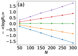
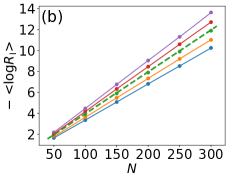
Figure 3: (Color online) (a) $-\langle\log R_{\rm T}\rangle$ and (b) $-\langle\log R_{\rm I}\rangle$ in the case of $g=0.02$ and $\gamma=0.0$ for $N$ ranging from $50$ to $300$, where $W/\Gamma=0.9$ (blue), $0.934$ (orange), $0.969$ (green), $1.002$ (red), and $1.036$ (violet) from bottom to top. In panel (b), a dashed line represents $-\langle\log R_{\rm I}\rangle=2g(N-1)$. Solid lines serve as visual guides.

We first examine the case of $g=0.02$ and $\gamma=0$ for $W/\Gamma=0.9$, $0.934$, $0.969$, $1.002$, and $1.036$. In the case of $\gamma=0$, the global conservation law (4) is reduced to

$$R_{\rm T}=e^{2g(N-1)}R_{\rm I},$$ (36)

which describes the amplification or attenuation of the injected probability current from the left lead owing to the asymmetry in $\Gamma_{\rm L}$ and $\Gamma_{\rm R}$. Figure 3(a) shows $-\langle\log R_{\rm T}\rangle$ as a function of $N$. A linear relationship between $-\langle\log R_{\rm T}\rangle$ and $N$ with a positive (negative) slope means that $R_{\rm T}$ decreases (increases) exponentially with increasing $N$. We observe from Fig. 3(a) that the slope of $-\langle\log R_{\rm T}\rangle$ changes from a negative value at $W/\Gamma=0.934$ to a positive value at $W/\Gamma=1.002$, whereas the slope is nearly flat at $W/\Gamma=0.969$. This shows that the delocalization–localization transition occurs at the critical value of $W_{\rm c}/\Gamma\approx 0.969$. Equation (36) indicates that if $-\langle\log R_{\rm T}\rangle$ is nearly flat, $-\langle\log R_{\rm I}\rangle$ increases with $N$ as $-\langle\log R_{\rm I}\rangle\approx 2g(N-1)$. This is consistent with the behavior of $-\langle\log R_{\rm I}\rangle$ shown in Fig. 3(b). Indeed, we observe in Fig. 3(b) that the data in the case of $W/\Gamma=0.969$ is on the dashed line of $-\langle\log R_{\rm I}\rangle=2g(N-1)$. Note that the behavior of $R_{\rm I}$ is identical to that of the transmission probability $T$ in the Hermitian limit of $g=0$ as shown in Appendix.

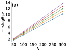
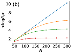
Figure 4: (Color online) (a) $-\langle\log R_{\rm T}\rangle$ and (b) $-\langle\log R_{\rm I}\rangle$ in the case of $g=0.0$ and $W/\Gamma=0.9$ for $N$ ranging from $50$ to $300$, where $\gamma/\Gamma=0.0$ (blue), $-0.002$ (orange), $-0.004$ (green), $-0.006$ (red), and $-0.008$ (violet) from bottom to top in panel (a), and $\gamma/\Gamma=0.0$ (blue), $-0.00001$ (orange), $-0.0001$ (green), and $-0.001$ (red) from top to bottom in panel (b). Solid lines serve as visual guides.

We next examine the case of $g=0$ at $W/\Gamma=0.9$ and several values of $\gamma$. Figure 4(a) shows $-\langle\log R_{\rm T}\rangle$ for $\gamma/\Gamma=0.0$, $-0.002$, $-0.004$, $-0.006$, and $-0.008$. We observe that $R_{\rm T}$ decreases exponentially as $N$ increases, and this exponential decrease becomes more rapid as $|\gamma|$ increases. Figure 4(b) shows $-\langle\log R_{\rm I}\rangle$ for $\gamma/\Gamma=0.0$, $-0.00001$, $-0.0001$, and $-0.001$. We observe that when $\gamma$ becomes finite ($|\gamma|>0$), the exponential decrease in $R_{\rm I}$ seen at $\gamma=0$ tends to stop at a finite value; $-\langle\log R_{\rm I}\rangle$ appears saturated at a sufficiently large $N$. Indeed, the behaviors of $R_{\rm T}$ and $R_{\rm I}$ are contrasting in the case of $\gamma\neq 0$. Unlike in the case of $R_{\rm T}$, the decrease in $R_{\rm I}$, after an initial exponential decrease, tends to be moderated, and $R_{\rm I}$ converges to a small but finite value. This lower limit of $R_{\rm I}$, which becomes vanishingly small as $\gamma\rightarrow 0$, increases with $|\gamma|$. Let us explain this feature in relation to Eq. (4), which is rewritten in the present case as

$$R_{\rm T}=R_{\rm I}+\sum_{n=1}^{N}\frac{\gamma\rho_{n}}{\Gamma\sin(ka)}.$$ (37)

For a sufficiently large $N$, $R_{\rm I}$ takes a value close to its lower limit, whereas $R_{\rm T}$ continues to decrease exponentially. In this regime, the dependence of $R_{\rm T}$ on $N$ is determined by the second term in Eq. (37), which represents the total amount of leakage due to the constant imaginary potential $i\gamma$. Assuming $\rho_{n}\propto\exp(-\frac{2n}{\xi})$ for $n\gg 1$ with a decay length $\xi$ normalized by $a$, we approximately express the second term in Eq. (37) with $\gamma<0$ as

$$\sum_{n=1}^{N}\frac{\gamma\rho_{n}}{\Gamma\sin(ka)}\sim A\exp\left(-\frac{2N}{\xi}\right)-B,$$ (38)

where $A>0$ is independent of $N$, whereas $B>0$ may weakly depend on $N$. In the Hermitian limit of $\gamma=0$, $\xi$ is identified as the localization length. We can explain the behaviors of $R_{\rm T}$ and $R_{\rm I}$ if $B$ cancels $R_{\rm I}$ (i.e., $B=R_{\rm I}$) on the right-hand side of Eq. (37). Thus, the first term on the right-hand side of Eq. (38) describes the exponential decrease in $R_{\rm T}$ as

$$R_{\rm T}\sim A\exp\left(-\frac{2N}{\xi}\right).$$ (39)

Since the exponential decrease in $\rho_{n}$ is enhanced by the leakage due to the constant imaginary potential $i\gamma$, the decay length $\xi$ decreases with increasing $|\gamma|$. This explains the behavior of $R_{\rm T}$ shown in Fig. 4(a). In turn, the leakage can occur only when the total amount of leakage, which is nearly equal to $B$, is supplied to the system from the left lead as indicated by $B=R_{\rm I}$. Hence, the injection rate $R_{\rm I}$ cannot continue to decrease with $N$, but tends to be bounded from below. The lower limit of $R_{\rm I}$ increases with increasing $|\gamma|$, since the total amount of leakage increases with $|\gamma|$. This explains the behavior of $R_{\rm I}$ shown in Fig. 4(b).

Figure 5: (Color online) (a) $-\langle\log R_{\rm T}\rangle$ and (b) $-\langle\log R_{\rm I}\rangle$ in the case of $g=0.02$ and $W/\Gamma=0.9$ for $N$ ranging from $50$ to $300$, where $\gamma/\Gamma=0.0$ (blue), $-0.002$ (orange), $-0.004$ (green), $-0.006$ (red), and $-0.008$ (violet) from bottom to top in panel (a), and $\gamma/\Gamma=0.0$ (blue), $-0.00001$ (orange), $-0.0001$ (green), and $-0.001$ (red) from top to bottom in panel (b). Solid lines serve as visual guides.

Finally, we examine the case of $g=0.02$ at $W/\Gamma=0.9$ and several values of $\gamma$. Figure 5(a) shows $-\langle\log R_{\rm T}\rangle$ for $\gamma/\Gamma=0.0$, $-0.002$, $-0.004$, $-0.006$, and $-0.008$. We observe from Fig. 5(a) that the slope of $-\langle\log R_{\rm T}\rangle$ changes from a negative value at $\gamma/\Gamma=-0.002$ to a positive value at $\gamma/\Gamma=-0.006$, whereas the slope is nearly flat at $\gamma/\Gamma=-0.004$. This shows that the delocalization–localization transition occurs at the critical value of $\gamma_{\rm c}/\Gamma\approx-0.004$. We also observe that, for each value of $\gamma$, the exponential decrease in $R_{\rm T}$ is slower than that in the case of $g=0$ shown in Fig. 4(a). This is again explained by using Eq. (4), which is rewritten in this case as

$$R_{\rm T}=e^{2g(N-1)}R_{\rm I}+\sum_{n=1}^{N}\frac{e^{2g(N-n)}\gamma\rho_{n}}{\Gamma\sin(ka)}.$$ (40)

Assuming $\rho_{n}\propto\exp[-2(\frac{1}{\xi}-g)n]$ for $n\gg 1$, we approximately express the second term in Eq. (40) with $\gamma<0$ as

$$\sum_{n=1}^{N}\frac{e^{2g(N-n)}\gamma\rho_{n}}{\Gamma\sin(ka)}\sim A^{\prime}\exp\left[-2\left(\frac{1}{\xi}-g\right)N\right]-e^{2gN}B^{\prime},$$ (41)

where $A^{\prime}>0$ is independent of $N$, whereas $B^{\prime}>0$ may weakly depend on $N$. Again, $e^{2gN}B^{\prime}$ should cancel $e^{2g(N-1)}R_{\rm I}$ on the right-hand side of Eq. (40) to give the exponential decrease in $R_{\rm T}$. We then find

$$R_{\rm T}\sim A^{\prime}\exp\left[-2\left(\frac{1}{\xi}-g\right)N\right].$$ (42)

Since the decay length $\xi$ decreases with increasing $|\gamma|$, this explains the behavior of $R_{\rm T}$ shown in Fig. 5(a). Figure 5(b) shows $-\langle\log R_{\rm I}\rangle$ for $\gamma/\Gamma=0.0$, $-0.00001$, $-0.0001$, and $-0.001$. The results shown in this figure are the same as those shown in Fig. 4(b) because $R_{\rm I}$ in the case of $g=0.02$ with a given $\gamma$ is identical to that in the case of $g=0$ with the same $\gamma$ as shown in Appendix.

6 Concluding remarks

In a mesoscopic length scale, transport through a conductor is characterized by the transmission and reflection probabilities, which are found by solving the corresponding scattering problem. Here, we have considered a non-Hermitian conductor connected to two Hermitian leads in a standard two-terminal setup. As a concrete Hamiltonian describing a non-Hermitian conductor, we have considered a generic non-Hermitian model with Hatano–Nelson-type asymmetric hopping and analyzed the corresponding non-Hermitian scattering problem. We have seen that the Hermitian interpretation of the scattering problem based on the transmission and reflection probabilities fails in this case. Introducing the incoming and outgoing currents [see Eqs. (19) and (20)], we have proposed the modified continuity equation (18) with Eq. (22), which serves as a local conservation law. The global probability conservation law (23) is derived from this local conservation law. We have tested the usefulness of our global probability conservation law in the interpretation of numerical experiments on non-Hermitian localization and delocalization phenomena.

We have seen that transport through a non-Hermitian system in the two-terminal setup is beyond a two-terminal description based on the Landauer formula. This is because an effective current is either injected from or leaked to a hypothetical external reservoir assumed to be existing in the underlying Hermitian model [see Fig. 1(b)]. Such a situation may be more appropriately described by a multiterminal Landauer formula [37] and will deserve a more thorough discussion in a future work.

Related to this, a microscopic derivation of the non-Hermitian effective Hamiltonian (9), or Eq. (7), will also deserve a thorough discussion. In the original paper of Hatano and Nelson, [26] the effective Hamiltonian (7) has been introduced to describe the depinning of a flux line driven by a perpendicular magnetic field in a cylindrical superconducting shell with columnar pinning centers. In the present context, Eq. (9) is expected to describe a one-dimensional Hermitian electron system coupled with an external reservoir [see Fig. 1(b)]. An important problem left for a future study is to determine the circumstances under which the use of the effective Hamiltonian is fully justified. A non-Hermitian electron system governed by Eq. (7) may be realized if each pair of nearest neighbor sites in the system are coupled with a reservoir in a particular manner. [29, 30, 31]

Appendix

In implementing the asymmetry in $\Gamma_{\rm R}$ and $\Gamma_{\rm L}$, we set $\Gamma_{\rm R}=e^{g}\Gamma$ and $\Gamma_{\rm L}=e^{-g}\Gamma$, [26, 27] which is equivalent to assuming $\Gamma_{\rm R}\Gamma_{\rm L}=\Gamma^{2}$. Under this setting, it is useful to introduce the similarity transformation

$$\Lambda=\sum_{n}|n\rangle b_{n}\langle n|$$ (43)

with

$$b_{n}=\left\{\begin{array}[]{cc}1&(n\leq 0),\\ e^{-g(n-1)}&(1\leq n\leq N),\\ e^{-g(N-1)}&(N+1\leq n).\end{array}\right.$$ (47)

We can show that $H$ is transformed to $\Lambda H\Lambda^{-1}=H_{g=0}$, where $H_{g=0}$ represents the Hamiltonian with $\Gamma_{\rm R}=\Gamma_{\rm L}=\Gamma$. Let us compare the stationary scattering state $|\psi_{g=0}\rangle$ satisfying $H_{g=0}|\psi_{g=0}\rangle=E|\psi_{g=0}\rangle$ and the stationary scattering state $|\psi\rangle$ satisfying $H|\psi\rangle=E|\psi\rangle$. The relation $\Lambda H\Lambda^{-1}=H_{g=0}$ ensures

$$|\psi_{g=0}\rangle=\Lambda|\psi\rangle,$$ (48)

which shows that, in the left lead of $n\leq 0$, $|\psi_{g=0}\rangle$ is identical to $|\psi\rangle$ since $b_{n}=1$. This means that, for the given $\gamma$ and disorder potential $V_{n}$, $R_{\rm I}$ associated with $|\psi\rangle$ is identical to that associated with $|\psi_{g=0}\rangle$. This statement relies on the similarity transformation; thus, it does not exactly hold in the case of $\Gamma_{\rm R}\Gamma_{\rm L}\neq\Gamma^{2}$, although Eq. (4) still holds.

References

- [1] I. Rotter, J. Phys. A: Math. Theor. 42, 153001 (2009).
- [2] Y. Ashida, Z. Gong, and M. Ueda, Adv. Phys. 69, 249 (2020).
- [3] R. E. Le Levier and D. S. Saxon, Phys. Rev. 87, 40 (1952).
- [4] H. Feshbach, C. E. Porter, and V. F. Weisskopf, Phys. Rev. 96, 448 (1954).
- [5] P. E. Hodgson, Rep. Prog. Phys. 47, 613 (1984).
- [6] A.A. Andrianov, M.V. Ioffe, F. Cannata, and J.-P. Dedonder, Int. J. Mod. Phys. A 14, 2675 (1999).
- [7] G. Lévai, F. Cannata, and A. Ventura J. Phys. A 34, 839 (2001).
- [8] R. N. Deb, A. Khare, and B. D. Roy, Phys. Lett. A 307, 215 (2003).
- [9] J. G. Muga, J. P. Palao, B. Navarro, and I. L. Egusquiza, Phys. Rep. 395, 357 (2004).
- [10] F. Cannata, J.-P. Dedonder, and A. Ventura, Ann. Phys. 322, 397 (2007).
- [11] H. F. Jones, Phys. Rev. D 76, 125003 (2007).
- [12] M. Znojil, Phys. Rev. D 78, 025026 (2008).
- [13] N. Hatano, K. Sasada, H. Nakamura, and T. Petrosky, Prog. Theor. Phys. 119, 187 (2008).
- [14] L. Jin and Z. Song, Phys. Rev. A 85, 012111 (2012).
- [15] K. Abhinav, A. Jayannavar, and P. K. Panigrahi, Ann. Phys. 331, 110 (2013).
- [16] N. Hatano, Fortschr. Phys. 61, 238 (2013).
- [17] P. A. Kalozoumis, G. Pappas, F. K. Diakonos, and P. Schmelcher, Phys. Rev. A 90, 043809 (2014).
- [18] S. Garmon, M. Gianfreda, and N. Hatano, Phys. Rev. A 92, 022125 (2015).
- [19] B. Zhu, R. Lü, and S. Chen, Phys. Rev. A 93, 032129 (2016).
- [20] A. Ruschhaupt, T. Dowdall, M. A. Simón, and J. G. Muga, EPL 120 20001 (2017).
- [21] P. C. Burke, J. Wiersig, and M. Haque, Phys. Rev. A 102, 012212 (2020).
- [22] K. Shobe, K. Kuramoto, K.-I. Imura, and N. Hatano, Phys. Rev. Research 3, 013223 (2021).
- [23] If is not normalizable as in the case of a stationary scattering state, cannot be simply interpreted as the probability of finding an electron at the th site. However, if many stationary scattering states are superposed to obtain a wave packet that satisfies the normalization condition , the probabilistic interpretation is applicable to in a rigorous sense.
- [24] B. Bagchi, C. Quesne, and M. Znojil, Mod. Phys. Lett. A 16, 2047 (2001).
- [25] K. Shobe, “Spontaneous current, skin and proximity effects in non-Hermitian systems”, presented at IIS-Chiba Workshop on Non-Hermitian Quantum Mechanics (NH2019TD), 2019.
- [26] N. Hatano and D. R. Nelson, Phys. Rev. Lett. 77, 570 (1996).
- [27] N. Hatano and D. R. Nelson, Phys. Rev. B 56, 8651 (1997).
- [28] An alternative recipe is given in K. Kawabata, T. Numasawa, and S. Ryu, Phys. Rev. X 13, 021007 (2023). This recipe uses Eq. (4) with replaced with as an expression of probability current and therefore essentially differs from that we propose in this paper [see Eqs. (18)–(20)].
- [29] Z. P. Gong, Y. Ashida, K. Kawabata, K. Takasan, S. Higashikawa, and M. Ueda, Phys. Rev. X 8, 031079 (2018).
- [30] A. McDonald, R. Hanai, and A. A. Clerk, Phys. Rev. B 105, 064302 (2022).
- [31] P. Liu, X. Y. Zhang, X. Z. Hao, Y. H. Zhou, S. C. Hou, and X. X. Yi, Phys. Rev. A 107, 053515 (2023).
- [32] M. Brandenbourger, X. Locsin, E. Lerner, and C. Coulais, Nat. Commun. 10, 4608 (2019).
- [33] S. Weidemann, M. Kremer, T. Helbig, T. Hofmann, A. Stegmaier, M. Greiter, R. Thomale, and A. Szameit, Science 368, 311 (2020).
- [34] T. Helbig, T. Hofmann, S. Imhof, M. Abdelghany, T. Kiessling, L. W. Molenkamp, C. H. Lee, A. Szameit, M. Greiter, and R. Thomale, Nat. Phys. 16, 747 (2020).
- [35] L. S. Palacios, S. Tchoumakov, M. Guix, I. Pagonabarraga, S. Sánchez, and A. G. Grushin, Nat. Commun. 12, 4691 (2021).
- [36] R. Landauer, Philos. Mag. 21, 863 (1970).
- [37] M. Büttiker, Y. Imry, R. Landauer, and S. Pinhas, Phys. Rev. B 31, 6207 (1985).