Online Sensitivity Optimization in Differentially Private Learning

Abstract

Training differentially private machine learning models requires constraining an individual’s contribution to the optimization process. This is achieved by clipping the $2$-norm of their gradient at a predetermined threshold prior to averaging and batch sanitization. This selection adversely influences optimization in two opposing ways: it either exacerbates the bias due to excessive clipping at lower values, or augments sanitization noise at higher values. The choice significantly hinges on factors such as the dataset, model architecture, and even varies within the same optimization, demanding meticulous tuning usually accomplished through a grid search. In order to circumvent the privacy expenses incurred in hyperparameter tuning, we present a novel approach to dynamically optimize the clipping threshold. We treat this threshold as an additional learnable parameter, establishing a clean relationship between the threshold and the cost function. This allows us to optimize the former with gradient descent, with minimal repercussions on the overall privacy analysis. Our method is thoroughly assessed against alternative fixed and adaptive strategies across diverse datasets, tasks, model dimensions, and privacy levels. Our results indicate that it performs comparably or better in the evaluated scenarios, given the same privacy requirements.

Introduction

The widespread adoption of machine learning techniques has led to increased concerns about user privacy. Users who share their data with service providers are becoming more cautious due to the exposure of various privacy attacks, observed in both academic and industrial contexts (Carlini et al. 2021, 2023; Papernot et al. 2018). As a result, there is a growing effort to enhance training methods that can provide strong and quantifiable privacy guarantees.

In the privacy-preserving machine learning community, differential privacy (Dwork 2006) has emerged as the predominant framework for defining privacy requirements and strategies. Essentially, training a model with differential privacy requires bounding the contribution of a single individual to the overall procedure, to guarantee that the trained model will be probabilistically indistinguishable compared to the same model trained without including any one specific user in the dataset. In the context of gradient-based learning, this is achieved by introducing a parameter $C$ called the clipping threshold (Abadi et al. 2016). This parameter controls the magnitude of gradients from each user (or sample) before they are averaged with contributions from other users. Subsequently, the result undergoes a process of differential privacy sanitization, which involves the addition of random Gaussian noise proportional to the value of $C$.

The choice of the clipping threshold $C$ is crucial: on the one hand, large values introduce noise levels that may slow down or hinder the optimization altogether; on the other hand, small values introduce a bias in the average clipped gradient with respect to the true average gradient and may leave the optimization stuck in bad local minima. Figure 1 exemplifies the issue. Note that the clipping bias is not only directed toward zero (as bounding the $2$-norm may lead to believe), but depends, in general, on the distribution of the per-sample gradients around the expectation (Chen, Wu, and Hong 2020). Achieving an optimal trade-off remains an ongoing challenge. Historically, researchers have treated the clipping threshold as a parameter to be optimized, often through a grid or random search, in order to assess the performance of privacy preserving models in the ideal conditions in which an oracle provides the optimal values for the hyperparameters. However, it is worth noting that every additional gradient-query to the dataset for optimization purposes introduces a certain degree of privacy leakage. Of late though, the implications of not accounting for privacy leakage over multiple runs of a grid search have drawn more attention, leading to different accounting strategies (Papernot and Steinke 2022; Mohapatra et al. 2022; Liu and Talwar 2019). The inherent challenges of increased privacy leakage and computational overhead resulting from extensive hyperparameter searches persist, necessitating further innovations to encourage broader adoption of differentially private machine learning techniques. Therefore, we set out to find a strategy for the online optimization of the clipping threshold that is privacy preserving and computationally inexpensive, while maintaining comparable or better performance on a set of tasks, datasets, and model architectures.

Our contributions: i) We investigate the sensitivity trade-off in differentially private learning in terms of cosine similarity between the sanitized and true gradients, showing that at every iteration it is possible to determine a fairly prominent optimal value, ii) we elaborate a strategy for the online optimization of the sensitivity, taking from the literature in online learning rate optimization and extending it to optimize the clipping threshold, iii) we establish the corresponding techniques for doing so privately, which require allocating a marginal privacy budget and iii) we provide experimental results to validate our algorithm in multiple contexts and against a number of relevant state-of-the-art strategies for private hyperparameter optimization.

Figure 1: The choice of clipping threshold $C$ requires trading off a higher clipping bias at small values, for larger Gaussian noise at large values. Here the clipped, averaged, noised gradient of a CNN for character recognition is compared with the true average gradient at different training iterations $t\in\{100,250,500,750,950\}$. Note that for some values the sanitized gradient may even have components pointing in the opposite direction w.r.t the true gradient, corresponding to negative cosine similarity. The reported figure of cosine similarity is an average over $20$ realizations of the Gaussian mechanism.

Background

Gradient-based optimization of supervised machine learning models typically implies finding the optimal set of parameters $\theta\in\mathbb{R}^{n}$ to fit a function $f_{\theta}:\mathcal{X}\rightarrow\mathcal{Y}$ to a dataset $D\in\mathcal{D}$ of pairs $z_{i}=(x_{i},y_{i})\in\mathcal{X}\times\mathcal{Y}$, by minimizing an error function $\ell:\mathbb{R}^{n}\times\mathcal{D}\rightarrow\mathbb{R}_{\geq 0}$. At time $t$, the iterative optimization process computes the cost of mismatched predictions and updates the parameters towards the nearest local minimum of $\ell$ by repeated applications of the (stochastic) gradient descent algorithm $\theta_{t+1}\leftarrow\theta_{t}-\rho g_{t}$, with $\rho$ the learning rate, and

$$g_{t}=\frac{1}{|B|}\sum_{z_{i}\in B}\nabla_{\theta_{t}}\ell(f_{\theta_{t}}(x_{i}),y_{i})$$ (1)

being the average gradient of the error function with respect to the parameters, computed over the samples $z_{i}=(x_{i},y_{i})$ of the minibatch $B\subseteq D$.

As is now commonplace in the machine learning literature, privacy guarantees are provided within the framework of Differential Privacy (DP):

Definition 1 (Differential Privacy (Dwork 2006))

A randomized mechanism $\mathcal{M}:\mathcal{D}\rightarrow\mathcal{R}$ with domain $\mathcal{D}$ and range $\mathcal{R}$ satisfies $(\varepsilon,\delta)$ differential privacy if for any two datasets $D,D^{\prime}\in\mathcal{D}$ differing in at most one sample, and for any outputs $S\subseteq\mathcal{R}$ it holds that

$$\text{Pr}[\mathcal{M}(D)\in S]\leq e^{\varepsilon}\text{Pr}[\mathcal{M}(D^{\prime})\in S]+\delta$$ (2)

To fit machine learning optimization within the definition of a differentially private random mechanism (intended here in a broad sense to also include later generalizations (Dwork and Rothblum 2016; Mironov 2017)) the average gradient in Equation (1) is sanitized by means of the Gaussian mechanism (Dwork, Roth et al. 2014). In particular, if $h:\mathcal{X}\rightarrow\mathbb{R}^{n}$ is a function with $2$-norm sensitivity $S_{h}$, the DP approximation $\tilde{h}(x)$ of $h(x)$, $x\in\mathcal{X}$, can be found as

$$\tilde{h}(x)=h(x)+\eta,\quad\eta\sim\mathcal{N}(0,\sigma^{2}I=S_{h}^{2}\nu^{2}I)$$ (3)

with $\nu$ the noise multiplier which depends only on the privacy parameters, and $\mathcal{N}$ being a random normal distribution. Tuning the additive Gaussian noise implies tuning its standard deviation proportionally to the $2$-norm sensitivity of the query $g_{t}$ over the minibatch $B$. As, in general, $\left\|g_{t}\right\|_{2}$ is not bounded a priori, the per-sample gradients of the error function are clipped in norm to a certain value $C_{t}$ (Song, Chaudhuri, and Sarwate 2013; Bassily, Smith, and Thakurta 2014; Shokri and Shmatikov 2015; Abadi et al. 2016) by applying the transformation

$$\bar{g}_{t}(z_{i})=\frac{g_{t}(z_{i})}{\text{max}\left(1,\frac{\left\|g_{t}(z_{i})\right\|_{2}}{C_{t}}\right)}$$ (4)

from which follows the sensitivity of the average clipped gradient, allowing for the sanitization of the query at the $t^{\text{th}}$ iteration. The Gaussian mechanism lends itself to a refined analysis of the privacy leakage incurred in its repeated application, which is essential in practical machine learning with stochastic gradient descent to keep the overall privacy expenditure to a minimum over multiple training epochs (Abadi et al. 2016; Wang, Balle, and Kasiviswanathan 2019). A similar procedure can be utilized to account for multiple runs with different configurations in a grid search (Mohapatra et al. 2022).

Related Works

This work draws from two main lines of research, namely hyperparameter optimization in non-private settings and sensitivity optimization in differentially private machine learning.

Hyperparameter Optimization

Sub-gradient minimization strategies such as SGD iteratively approach the optimal solution by taking steps in the direction of steepest descent of a cost function. For this heuristic to be effective, the length of each step needs to be tuned by controlling the learning rate, which has been considered the “single most important hyperparameter” (Bengio 2012). Many works have introduced strategies for its adaptive tuning, such as (Lydia and Francis 2019; Kingma and Ba 2014), which adjust the per-parameter value w.r.t. a common value still defined a priori. Conversely, other research has exploited automatic differentiation to concurrently optimize the parameters and hyperparameters (Maclaurin, Duvenaud, and Adams 2015) via SGD. In particular, explicitly deriving the partial derivative of the cost function with respect to the learning rate has been demonstrated to be an effective strategy, and it has been discovered independently at different times (Almeida et al. 1999; Baydin et al. 2018). These works do not explore the private setting and introduce general methods that are almost exclusively applied to learning rate optimization, without addressing the choice of other hyperparameters. In (Mohapatra et al. 2022) instead, the authors study adaptive optimizers in the differentially private setting, by analyzing the estimate of the raw second moment of the gradient at convergence. Their objective is to reduce the privacy cost of tuning the learning rate in a grid search, but the clipping threshold is still treated as an additional hyper-parameter.

Sensitivity Optimization

As discussed in the Introduction and Background sections, establishing the value of the clipping threshold $C_{t}$ is critical in differentially private machine learning, and treating this value as a hyper-parameter has largely been the preferred strategy in the literature (Song, Chaudhuri, and Sarwate 2013; Bassily, Smith, and Thakurta 2014; Shokri and Shmatikov 2015; Abadi et al. 2016). Grid searching over the candidate values can be tricky as gradient norms may span many orders of magnitude and the effects of more aggressive clipping are not easily predicted before running an optimization. Considering also the increased privacy costs of running multiple configurations, hyperparameter selection under privacy constraints is a thriving research area (Papernot and Steinke 2022; Liu and Talwar 2019; Mohapatra et al. 2022).

Adaptive clipping strategies have also been considered. (Andrew et al. 2021) updates $C_{t}$ during training to match a target quantile of the gradient norms, which is fixed beforehand. Although the optimal quantile is still a hyper-parameter, its domain is limited to the $[0,1]\subset\mathbb{R}$ interval. Moreover, (Andrew et al. 2021) shows that adaptively updating $C_{t}$ outperforms even the best fixed-clipping strategy. Additionally, as DP training has shown to disproportionally favor majority classes in a dataset (Suriyakumar et al. 2021), tuning a target quantile instead of a fixed clipping threshold may help at least in quantifying the issue, if not in solving it. Note that although this strategy was introduced to train differentially private federated machine learning models, the attacker is still modelled as an honest-but-curious adversary and thus it relies on a central trusted server to provide DP guarantees. Therefore, the clipping strategy in (Andrew et al. 2021) can be used to train centralized machine learning models just by switching from user-level to sample-level differential privacy (McMahan et al. 2018b). To further stress this point, note that although in (Andrew et al. 2021) each single user clips the update and sends statistics to the central server, from a differential privacy point of view this is identical to the server performing these operations itself on the true per-user gradients.

Method

Inspired by the literature on online hyperparameter optimization discussed in the Related Works, the idea behind this method is to optimize the clipping threshold based on the chain rule for derivatives, so that we can find what change in $C_{t}$ will induce a decrease in the cost function $\ell(\theta_{t})$. Although this strategy works in general for sub-gradient methods, we are going to explicitly derive the results for DP-SGD. Given the SGD update rule with gradient clipping:

$$\theta_{t+1} =\theta_{t}-\rho\nabla\ell(\theta_{t})$$ (5)

$$=\theta_{t}-\rho\frac{1}{|B_{t}|}\sum_{z_{i}\in B_{t}}\frac{g_{t}(z_{i})}{\max(1,\left\|g_{t}(z_{i})\right\|_{2}/C_{t})}$$ (6)

we want to find

$$\frac{\partial\ell(\theta_{t})}{\partial C} =\frac{\partial\ell(\theta_{t})}{\partial\theta_{t}}^{\top}\frac{\partial\theta_{t}}{\partial C_{t}}$$ (7)

$$=\nabla\ell(\theta_{t})^{\top}\frac{\partial\theta_{t}}{\partial C_{t}}$$ (8)

$$=-\rho\nabla\ell(\theta_{t})^{\top}\frac{\partial\nabla\ell(\theta_{t-1})}{\partial C_{t-1}}$$ (9)

where in the last equality we exploit $\theta_{t}=\theta_{t-1}-\rho\nabla\ell(\theta_{t-1})$ and assume $C_{t}\approx C_{t-1}$. To find an explicit form for Equation (9), we notice that the rightmost term is differentiable almost everywhere, with:

$$\frac{\partial\nabla\ell(\theta_{t-1})}{\partial C_{t-1}}=q_{t-1}=\frac{1}{|B_{t-1}|}\sum_{z_{i}\in B_{t-1}}q_{t-1}(z_{i})$$ (10)

and

$$q_{t-1}(z_{i})=\begin{cases}\frac{g_{t-1}(z_{i})}{\left\|g_{t-1}(z_{i})\right\|_{2}}&\text{if}\left\|g_{t-1}(z_{i})\right\|_{2}>C_{t-1}\\ 0&\text{otherwise}\end{cases}$$ (11)

where we highlight that $\left\|q_{t-1}(z_{i})\right\|_{2}\in\{0,1\},\forall z_{i}\in B_{t-1}$ by definition of the clipping function. Thus we find:

$$\frac{\partial\ell(\theta_{t})}{\partial C_{t}}=-\rho\nabla\ell(\theta_{t})^{\top}\frac{1}{|B_{t-1}|}\sum_{z_{i}\in B_{t-1}}q_{t-1}(z_{i})$$ (12)

resulting in the gradient descent update rule for the clipping threshold:

$$C_{t+1}=C_{t}+\rho_{c}\rho\nabla\ell(\theta_{t})^{\top}\frac{1}{|B_{t-1}|}\sum_{z_{i}\in B_{t-1}}q_{t-1}(z_{i})$$ (13)

which is the dot product of the current average gradient with a masked version of last iteration’s average gradient, where all per-sample gradients have either norm $0$ or $1$.

Taking into account the coupled dynamics of the learning rate and the clipping threshold (Mohapatra et al. 2022), having an adaptive clipping strategy may still slow down convergence if the learning rate is kept fixed at the starting value. Thus, we use the same method to derive an update strategy for the learning rate $\rho_{t}$, as in (Almeida et al. 1999; Baydin et al. 2018):

$$\frac{\partial\ell(\theta_{t})}{\partial\rho_{t}} =\frac{\partial\ell(\theta_{t})}{\partial\theta_{t}}^{\top}\frac{\partial\theta_{t}}{\partial\rho_{t}}$$ (14)

$$=\nabla\ell(\theta_{t})^{\top}\nabla\ell(\theta_{t-1})$$ (15)

which results in the dot product of the current and past clipped gradients, yielding:

$$\rho_{t+1}=\rho_{t}+\rho_{r}\rho\nabla\ell(\theta_{t})^{\top}\nabla\ell(\theta_{t-1})$$ (16)

We do not further expand this result for brevity and because computing these quantities does not require a dedicated procedure, as they are already a byproduct of SGD to optimize $\theta_{t}$, even in a non-private setting.

Privacy Analysis

When assuming a time-dependent $C_{t}$ such as in (Andrew et al. 2021), it is particularly useful to decouple the contributions of the sensitivity from contributions of the privacy parameters $(\varepsilon,\delta)$ to the variance of the Gaussian mechanism, as in Equation (3). Then, within the framework of Rényi DP and given the results in (Mironov 2017; Wang, Balle, and Kasiviswanathan 2019) one can efficiently determine ahead of training-time the values of noise multiplier to be applied at each iteration independently of the current value of $C_{t}$. At the $t^{\text{th}}$ iteration there may be two sources of differential privacy leakage: the computation of $\theta_{t+1}$ in Equation (5) and the computation of $C_{t+1}$ in Equation (13). Both can be sanitized with the DP approximation already discussed, but the latter needs special attention. To sanitize $C_{t+1}$ with the Gaussian mechanism (for reasons detailed in Proposition 1) we may utilize $\nabla\ell(\theta_{t})\approx\nabla\tilde{\ell}(\theta_{t})$, effectively repurposing the sanitized gradient with respect to $\theta_{t}$. We focus now on the non-privatized term $\partial\nabla\ell(\theta_{t-1})/\partial C_{t-1}$. Naturally, it still involves the sanitization of a sum of vectors, with the fortunate benefit of having all the terms in the summation be of norm either $0$ or $1$, as shown in Equation (11), resulting in the unit sensitivity of the query. Thus, this step does not introduce the need to develop any further “higher order” (adaptive) clipping strategies. With the considerations above, from a privacy perspective, the two privatized parallel queries behave as a single query sanitized with the Gaussian mechanism. This result is formalized in Proposition 1, which follows from the joint clipping strategy described in (McMahan et al. 2018a).

Proposition 1

The Gaussian approximations $\tilde{q}_{t}$ and $\tilde{g}_{t}$ of $\sum_{z_{i}\in B_{t-1}}q_{t-1}(z_{i})$ and $\sum_{z_{i}\in B_{t}}\bar{g}_{t}(z_{i})$ with noise multipliers, respectively, $\nu_{q}$ and $\nu_{g}$, is equivalent (as far as privacy accounting is concerned) to the application of a single Gaussian mechanism with noise multiplier $\nu$ if $\nu_{g}=(\nu^{-2}-\nu_{q}^{-2})^{-1/2}$.

Compared to Theorem 1 in (Andrew et al. 2021), we lose a factor of $2$ in the reduction of the standard deviation $\sigma_{q}=1\cdot\nu_{q}$ and since $\nu_{q}$ is used here to sanitize a sum of vectors in $\mathbb{R}^{n}$ (whereas (Andrew et al. 2021) only need to sanitize a scalar quantity) we cannot relegate as much differentially private noise to the computation of $\tilde{q}_{t}$. Nonetheless, we can derive a rule of thumb, which, together with practical considerations introduced in the next section, allow to have working estimates of the true $\partial\ell(\theta_{t})/\partial C_{t}$. In particular, if we allow a $1\%$ increase in $\nu_{g}$ over $\nu$, we can rearrange the result in Proposition 1 to find $\nu_{q}\approx 7.124\cdot\nu$. Figure 2 shows an example of these trade-offs for the MNIST dataset discussed in Experiments section.

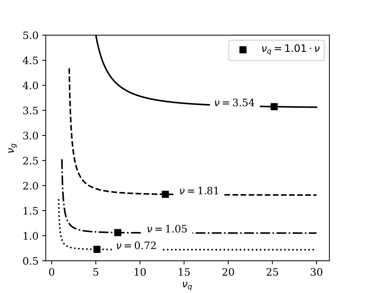
Figure 2: The Pareto frontiers of the noise multipliers to sanitize $\tilde{g}_{t}$ and $\tilde{q}_{t}$, and the chosen values given the heuristic described in the Privacy Analysis section, at different privacy requirements. This particular instance comes from the MNIST experiments described in the Experiments section.

To complete the privacy analysis, we highlight that from a DP point of view, the updates to the learning rate described in Equation (16) come with no additional privacy expenditure with respect to DP-SGD, exploiting the sanitized $\tilde{g}_{t}$ and $\tilde{g}_{t-1}$.

The OSO-DPSGD Algorithm

The algorithm keeps track of two sanitized quantities at each iteration, that is:

$$\tilde{q}_{t}=\frac{1}{|B_{t}|}\sum_{z_{i}\in B_{t}}q_{t}(z_{i})+\eta,\quad\eta\sim\mathcal{N}(0,\nu_{q}^{2}I)$$ (17)

$$\tilde{g}_{t}=\frac{1}{|B_{t}|}\sum_{z_{i}\in B_{t}}\bar{g}_{t}(z_{i})+\eta,\quad\eta\sim\mathcal{N}(0,C_{t}^{2}\nu_{g}^{2}I)$$ (18)

from which one can privately compute the parameter update and $\partial\tilde{\ell}(\theta_{t})/\partial C_{t}=-\rho\tilde{g}_{t}^{\top}\tilde{q}_{t-1}$, which requires to store $\tilde{q}_{t-1}$ from the last iteration. Note that storing vectors from past iterations is a common strategy even in non-privatized learning, as e.g. it is required by every optimizer with momentum(s). In order to cater to the wide range of values $C_{t}$ might take, spanning orders of magnitude (Andrew et al. 2021), instead of relying on the additive update rule in Equation (13), we first consider the scale-invariant Equation (19) proposed in (Rubio 2017), which converges with a logarithmic number of steps, instead of linearly

$$C_{t+1}=C_{t}\cdot\left(1+\rho_{c}\frac{\tilde{g}_{t}{}^{\top}\tilde{q}_{t-1}}{\left\|\tilde{g}_{t}\right\|_{2}\left\|\tilde{q}_{t-1}\right\|_{2}}\right)$$ (19)

We briefly experimented with Equation (19) and found the proportional update step $\tilde{g}_{t}{}^{\top}\tilde{q}_{t-1}/\left\|\tilde{g}_{t}{}^{\top}\tilde{q}_{t-1}\right\|_{2}=\text{sign}(\tilde{g}_{t}{}^{\top}\tilde{q}_{t-1})$ to be more robust w.r.t. the Gaussian noise and less dependent on the particular choice of $\rho_{c}$. Noticing that $1+x\approx e^{x}$ for small values of $x$, we converge to an exponential update rule for the optimization of both $C_{t}$ and $\rho_{t}$, similar to (Andrew et al. 2021):

$$C_{t+1}=C_{t}\cdot\text{exp}(\rho_{c}\text{sign}(\tilde{g}_{t}{}^{\top}\tilde{q}_{t-1}))$$ (20)

$$\rho_{t+1}=\rho_{t}\cdot\text{exp}(\rho_{r}\text{sign}(\tilde{g}_{t}{}^{\top}\tilde{g}_{t-1}))$$ (21)

Although we provide the result for vanilla SGD, deriving the update rule for the case with first order momentum is trivial and only adds a multiplicative factor to $\partial\ell/\partial C$, depending on the specific implementation of momentum. The same analysis for Adam is more involved and most importantly it results in the summation in $\partial\nabla\ell(\theta_{t-1})/\partial C_{t-1}$ to lose the appealing property of unitary sensitivity. Considering also the disparate results of Adam as a DP optimizer (Mohapatra et al. 2022; Andrew et al. 2021), we leave this analysis for future work. Finally, Algorithm 1 outlines the online optimization strategy presented above, which we call OSO-DPSGD.

1:Inputs Samples $z_{i}\in D$; $\rho$; $T$; $C_{0}$; $\theta_{0}$; $|B|$; per-iteration noise multiplier $\nu$; $\nu_{q}$; $\rho_{c}$; $\rho_{r}$; $\tilde{q}_{0}=\tilde{g}_{0}=0$.

2:$\nu_{g}\leftarrow(\nu^{-2}-\nu_{q}^{-2})^{-1/2}$

3:for $t\in\{1,\dots,T\}$ do

4:     $B_{t}\leftarrow$ draw $|B|$ samples uniformly from $D$

5:     for $z_{i}\in B_{t}$ in parallel do

6:         $g_{t}(z_{i})\leftarrow\nabla_{\theta_{t}}\ell(\theta_{t},z_{i})$

7:         $\bar{g}_{t}(z_{i})\leftarrow g_{t}(z_{i})/\text{max}(1,\frac{\left\|g_{t}(z_{i})\right\|_{2}}{C_{t}})$

8:         $q_{t}(z_{i})\leftarrow\frac{g_{t}(z_{i})}{\left\|g_{t}(z_{i})\right\|_{2}}$ if $\left\|g_{t}(z_{i})\right\|_{2}>C_{t}$ else $0$

9:     end for

10:     $\sigma_{g}\leftarrow\nu_{g}C_{t}$

11:     $\tilde{g}_{t}\leftarrow\frac{1}{|B|}\left(\sum_{z_{i}\in B_{t}}\bar{g}_{t}(z_{i})+\mathcal{N}(0,I\sigma_{g}^{2})\right)$

12:     $\theta_{t+1}\leftarrow\theta_{t}-\rho\hat{g}_{t}$

13:     $\tilde{q}_{t}\leftarrow\frac{1}{|B|}\left(\sum_{z_{i}\in B_{t}}q_{t}(z_{i})+\mathcal{N}(0,I\nu_{g}^{2})\right)$

14:     $C_{t+1}\leftarrow C_{t}\text{exp}(\rho_{c}\text{sign}(\tilde{g}_{t}{}^{\top}\tilde{q}_{t-1}))$

15:     $\rho_{t+1}\leftarrow\rho_{t}\text{exp}(\rho_{r}\text{sign}(\tilde{g}_{t}{}^{\top}\tilde{g}_{t-1}))$

16:end for

Algorithm 1 Differentially private optimization with OSO-DPSGD

In Algorithm 1 we list the learning rates of $C_{t}$ and $\rho$ as hyperparameters. In practice, especially considering the exponential update rule in Equations (20) and (21), they can be set to the same value. After a qualitative exploration of reasonable values for both, we settle on $\rho_{c}=\rho_{r}=2.5\cdot 10^{-3}$ for all the experiments.

Experiments

In the following Section we proceed to assess Algorithm 1 on a range of experiments on different datasets, tasks, and model sizes. In particular, we explore how online sensitivity optimization can be an effective tool in reducing the privacy and computational costs of running large grid searches. In an effort to draw conclusions that can be as general as possible, we identify three vastly adopted datasets in the literature: MNIST (LeCun et al. 1998), FashionMNIST (Xiao, Rasul, and Vollgraf 2017), and AG News (Gulli 2005) (Zhang, Zhao, and LeCun 2015). They are used to train, respectively, a convolutional neural network for image classification, a convolutional autoencoder and a bag of words fully connected neural network for text classification. For further details on the models and their architecture, refer to the Appendix.

	AG News	MNIST	Fashion MNIST
Dataset Size	120000	60000	60000
Batch Size	512	512	512
Model Size	113156	551322	48705

Table 1: Dataset and model information shared throughout the experiments.

Considering the computational burden of benchmarking multiple grid searches, we devise the following pipeline:

• Define the different learning algorithms; to compare OSO-DPSGD with relevant strategies, we also include in our experiments the FixedThreshold of (Song, Chaudhuri, and Sarwate 2013) (Shokri and Shmatikov 2015) (Abadi et al. 2016) among others and FixedQuantile of (Andrew et al. 2021). As reported by the respective authors, hyperparameter optimization is performed via grid search over the learning rates and threshold values for the former and over the learning rates and the quantiles for the latter. Even though (Mohapatra et al. 2022) introduce AdamWOSM for the DP adaptive optimization of the learning rate, it still tackles the challenge of reducing the number of hyperparameters in a privacy-aware grid search, and therefore we include it.

• Establish the corresponding grid search ranges. In all of our experiments, we fix the ranges of the hyperparameters to the same values. Considering the variety of experiments, and without assuming any particular domain knowledge of the task at hand, we opt for large ranges: $C\in[10^{-2},10^{2}]$ for the clipping threshold, $\rho\in[10^{-2.5},10^{1.5}]$ for the learning rate and $\gamma\in[0.1,0.9]$ for the target quantile.

• Define grid searches with different granularity. Given the ranges defined in the last step, DP training introduces possibly yet another hyperparameter. In fact, increasing the granularity inevitably results in more candidates, and an additional trade off to consider is that of increased fine tuning at the cost of additional privacy leakage. In our experiments, we evaluate 3 grid searches with different granularity, i.e. from the $\rho$ and $C$ ranges in the last step we take $k\in\{5,7,9\}$ values uniformly separated in a logarithmic scale. For the experiments with the FixedQuantile strategy we keep the values $\gamma\in[0.1,0.3,0.5,0.7,0.9]$ defined by the authors in (Andrew et al. 2021), as well a setting the learning rate for the exponential update rule for $C$ to $0.2$. The initial value for the clipping threshold in both FixedQuantile and Online is set to $C_{0}=0.1$.

• Execute private hyperparameter optimization at different privacy levels. For the same $\delta$, we explore with increasing values of $\varepsilon$. Following (Mohapatra et al. 2022), the privacy budgets we establish are per-grid, and not per-run. That is, algorithms that need extra fine-tuning and additional parameters, resulting in more runs, will effectively reduce the per-run privacy budget. Although this setting may not conform to most past literature, we are motivated by approaching DP machine learning from the practitioner point of view, where an oracle providing the optimal hyperparameters may not be a reasonable assumption. As in (Mohapatra et al. 2022), we utilize the moment accountant to distribute the privacy budget among the configurations, as we do not have a large number of candidates.

On top of comparing DP learning strategies, we provide a baseline in the non-private setting, where we iterate only over the learning rate values and initial weights. To limit the contribution of the Gaussian random noise in the DP setting, each configuration is executed with $5$ different seeds, and the results are averaged. Runs with different seeds are not accounted for in terms of privacy budget. Given the large number of runs, we validate each model at training time every $50$ iterations on the full test set, and pick the model checkpoint at the best value as representative of the corresponding configuration. Each configuration runs for $10$ epochs regardless of when the best performance is registered. Given the model size and datasets, the total number of epochs is enough to have most configurations converge. Nevertheless, we don’t expect every combination of hyperparameters to saturate learning, e.g. when training with $C$ and $\rho$ both set at the lowest value available in the corresponding ranges. In Tables 2, 3, 4, we list the hyperparameters leading to the best results in the grid search with granularity $k=7$ for the corresponding datasets and models. For brevity, we include detailed results only for this specific setting in the main paper. Results for the remaining granularity values, as well as the numerical results shown graphically only for $k=7$, are deferred to the Appendix.

Discussion Figure 3 shows the accuracy of the models in the best configurations, among those tested, on the MNIST dataset. Even though at higher privacy levels (low $\varepsilon$) Online and AdamWOSM appear to be equivalent in terms of results, we can see the former showing better results when the privacy requirements are relaxed. A possible explanation may be found in Table 2 by noticing that the best $C$ value for AdamWOSM is fairly large compared to the other strategies. We believe that a larger initial value for $C$ may be positive to take long strides towards the direction of the average gradient at the early stages of the optimization, but may be detrimental towards the end when reducing the Gaussian noise may help the optimization. Nevertheless, we consider both strategies to be roughly equivalent in this experiment. The results for FixedThreshold and FixedQuantile are consistently lower, most likely due to both strategies needing a larger grid search, which in turn limits the per-run privacy budget. Perhaps more surprisingly, the adaptive strategy FixedQuantile does not seem to show better results compared to fixing the clipping threshold at the initial value. The improved results that are found in (Andrew et al. 2021) in the federated setting do not seem to translate in centralized learning, with the experiments we conducted.

	Online	Fixed Threshold		Fixed Quantile		Adam WOSM
$\varepsilon$	$\rho$	$\rho$	$C$	$\rho^{*}$	$\gamma$	$C$
3	0.3162	0.01467	1.0	3.162	0.5	21.54
5	1.467	0.003162	4.64	3.162	0.7	21.54
7	1.467	6.812	0.010	3.162	0.7	21.54
9	1.467	6.812	0.010	3.162	0.7	21.54

Table 2: Best hyperparameters for the MNIST dataset with grid search granularity $k=7$. Values with ^∗ are scaled $\times 10^{3}$ for better readability. Best NoDP result for $\rho=0.003162$.

	Online	Fixed Threshold		Fixed Quantile		Adam WOSM
$\varepsilon$	$\rho$	$\rho$	$C$	$\rho$	$\gamma$	$C$
1	0.3162	0.0681	0.010	-	-	0.01
2	1.467	1.467	0.010	0.3162	0.3	0.01
3	1.467	6.812	0.010	1.467	0.1	0.0464
4	1.467	1.467	0.0464	1.467	0.3	0.01

Table 3: Best hyperparameters for the Fashion MNIST dataset with grid search granularity $k=7$. Best NoDP result for $\rho=0.01467$. All FixedQuantile runs diverge for $\varepsilon=1$.

	Online	Fixed Threshold		Fixed Quantile		Adam WOSM
$\varepsilon$	$\rho$	$\rho$	$C$	$\rho*$	$\gamma$	$C$
3	0.06812	1.467	0.01	3.162	0.5	0.01
5	0.06812	1.467	0.010	3.162	0.5	0.01
7	0.06812	1.467	0.010	3.162	0.7	0.01
9	0.06812	0.03162	0.0464	3.162	0.7	0.01

Table 4: Best hyperparameters for the AG News dataset. Values with ^∗ are scaled $\times 10^{3}$ for better readability. $k=7$. Best NoDP result for $\rho=0.003162$.

Figure 4 shows the best results in terms of mean squared error on the FashionMNIST dataset, where a model is trained to encode and decode the input images of clothing items. The chosen architecture is based on a convolutional autoencoder, and it has the smallest number of parameters among those considered in this work, as in Table 1. The privacy regimes are then chosen accordingly. Firstly, we notice that for $\varepsilon=1$ the FixedQuantile strategy does not converge with any of the available hyperparameters. To justify this result, we highlight how in Table 3 all other strategies adopt aggressive clipping strategies with small $C$’s. We thus believe that for very high privacy regimes even running with $\gamma=0.1$ (the lowest value for the target quantile) may induce large swings in the exponential updates of $C_{t}$, disrupting the optimization. Nevertheless, for $\varepsilon\in\{2,3,4\}$ this strategy shows the second best results. Conversely, AdamWOSM may be penalized by the choice of the initial $\rho_{0}=10^{-3}$, as suggested by the authors in (Mohapatra et al. 2022). In fact, we notice from Table 4 that the optimal clipping threshold is very small in all competing strategies, and the combination of small $C$ and small $\rho_{0}$ may render the optimization excessively slow to converge within the set number of epochs. Further, it may suggest that adapting the learning rate on a per-parameter basis, as in AdamWOSM, can be effective as long as the base learning rate is itself carefully selected. Thus, optimizing $\rho_{t}$ in the grid search, and then adaptively tuning it within the same run, as done in Online, seems to show better results.

Figure 5 plots the accuracy on the AG News dataset, where a bag of words model with a fully connected neural network is used to classify a selection of news in one of four classes. In this experiment we notice that AdamWOSM performs the best, with Online being marginally below. Still, as with the MNIST dataset, we take both strategies to be comparable in these two settings, as the average of one roughly fits within a standard deviation of the other.

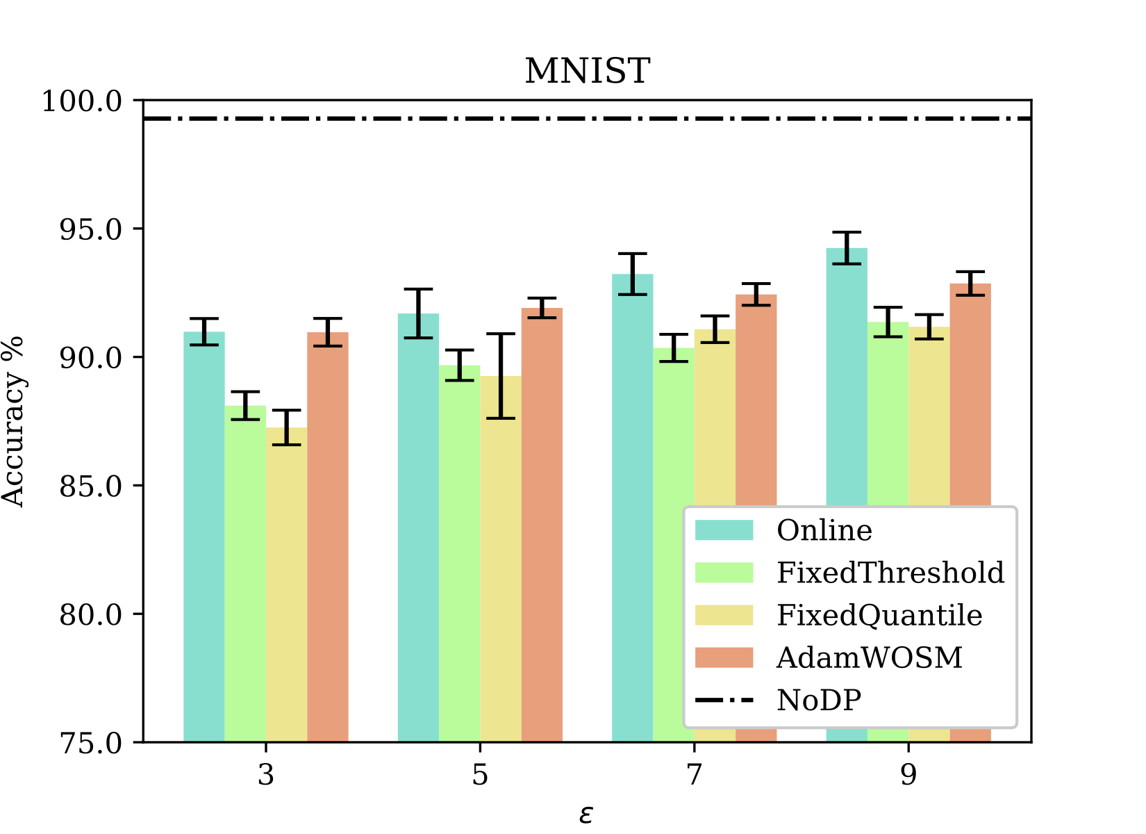
Figure 3: Accuracy on the MNIST dataset. Higher is better.

Figure 4: Mean Squared Error on the Fashion MNIST dataset. Lower is better. All runs for $\varepsilon=1$ of FixedQuantile result in a diverging optimization and are therefore not included.

Figure 5: Accuracy on the AG News dataset. Higher is better.

Conclusion

This work studies differentially private machine learning in the context of hyperparameter optimization, where the privacy cost of running a grid search is accounted for. Under these conditions, algorithms that require one less parameter may be preferable. Thus we explore strategies for the adaptive tuning of the clipping threshold $C$, and derive a result inspired by online learning rate optimization. With the proposed strategy, which we incorporate in the OSO-DPSGD algorithm, the clipping threshold is updated at each iteration based on the direction of steepest descent of the cost function. The resulting update rule is particularly clean, and results in the dot product between two sanitized vector queries: the average gradient at time $t$, and the derivative w.r.t. $C$ of the gradient at time $t-1$. With the former already needed in standard DP-SGD, and the latter resulting in a query with unitary sensitivity, the additional computational and privacy burden is minimal. Our range of experiments seems to encourage further research in this area, as online sensitivity optimization shows comparable results with one less parameter when assessed against standard state of the art algorithms, if the privacy guarantees are required at a grid search level, and not just within a single run. In the future, we hope to refine our analysis and algorithm, to possibly achieve better results even in this latter setting of per-run privacy requirements.

Appendix A Appendix - Models and Experiments

As mentioned in the corresponding Section of the main paper, we provide additional details about the model architectures, datasets, and results of experiments at different granularity levels. The model architectures are outlined in Tables 5, 6, 7. All datasets go through minor pre-processing, that is pixel values are mapped to the $[0,1]$ interval, while the text-based dataset AG News first goes through word embedding, using an embedding size of $50$ for up to the first $25$ words. To speed up development, we use the pre-trained word embeddings from (Pennington, Socher, and Manning 2014). Next, we report the results for granularity $k=5$ in Tables 11, 12 13 and Figures 9, 10 and 11. For $k=9$, results are presented in Tables 8, 9, 10 and Figures 6, 7 and 8.

CNN
layer	kernel size output size	stride	non linearity
2D Conv	$16\times 8\times 8$	$1\times 1$	ReLU
2D MaxPool	$2\times 2$	$1\times 1$	-
2D Conv	$32\times 4\times 4$	$1\times 1$	ReLU
Linear	$32$	-	ReLU
Linear	$10$	-	ReLU

Table 5: CNN

AutoEncoder
layer	kernel size output size	stride	non linearity
2D Conv	$8\times 3\times 3$	$1\times 1$	LeakyReLU
2D Conv	$16\times 3\times 3$	$1\times 1$	LeakyReLU
2D Conv	$32\times 3\times 3$	$1\times 1$	LeakyReLU
2D Conv	$64\times 3\times 3$	$1\times 1$	LeakyReLU
2D Transpose Conv	$32\times 3\times 3$	$1\times 1$	LeakyReLU
2D Transpose Conv	$16\times 3\times 3$	$1\times 1$	LeakyReLU
2D Transpose Conv	$8\times 3\times 3$	$1\times 1$	LeakyReLU
2D Transpose Conv	$1\times 3\times 3$	$1\times 1$	Sigmoid

Table 6: AutoEncoder

BagOfWords - FC
layer	output size	non linearity
Linear	$128$	LeakyReLU
Linear	$128$	LeakyReLU
Linear	$4$	LeakyReLU

Table 7: Bag of Words model architecture with a fully connected neural network.

Figure 6: $k=9$. Accuracy on the MNIST dataset. Higher is better. Refer to Table 8 for numeric results and optimized hyperparameters.

Figure 7: $k=9$. Mean Squared Error on the Fashion MNIST dataset. Lower is better. Refer to Table 9 for numeric results and optimized hyperparameters.

Figure 8: $k=9$. Accuracy on the AG News dataset. Higher is better. Refer to Table 10 for numeric results and optimized hyperparameters.

Figure 9: $k=5$. Accuracy on the MNIST dataset. Higher is better. Refer to Table 11 for numeric results and optimized hyperparameters.

Figure 10: $k=5$. Mean Squared Error on the Fashion MNIST dataset. Lower is better. Refer to Table 12 for numeric results and optimized hyperparameters.

Figure 11: $k=5$. Accuracy on the AG News dataset. Higher is better. Refer to Table 13 for numeric results and optimized hyperparameters.

	Online			Fixed Threshold				Fixed Quantile				Adam WOSM
$\varepsilon$	$\rho$	acc	std dev	$\rho$	$C$	acc	std dev	$\rho^{*}$	$\gamma$	acc	std dev	$C$	acc	std dev
3	0.316	90.69	0.53	100.0	0.1000	86.83	0.70	3.162	0.5	85.48	0.39	10.0	90.62	0.52
5	1.00	91.62	0.83	3.162	3.162	88.69	0.57	3.162	0.5	88.13	0.59	10.0	91.60	0.39
7	1.00	92.94	0.90	3162.0	0.0100	90.04	0.49	3.162	0.7	90.73	0.72	31.62	92.19	0.37
9	1.00	93.62	0.91	3.162	10.00	90.72	0.47	3.162	0.7	91.09	0.51	31.62	92.53	0.33

Table 8: MNIST, $k=9$, best NoDP for $\rho=0.003162$, ^∗ values are scaled $\times 10^{3}$.

	Online			Fixed Threshold				Fixed Quantile				Adam WOSM
$\varepsilon$	$\rho$	mse $\times 10^{2}$	std dev	$\rho$	$C$	mse $\times 10^{2}$	std dev	$\rho$	$\gamma$	mse $\times 10^{2}$	std dev	$C$	mse $\times 10^{2}$	std dev
1	0.100	2.57	0.29	0.0316	0.01	11.32	1.46	-	-	-	-	0.0100	4.48	0.83
2	1.000	0.94	0.13	0.100	0.01	12.35	1.87	0.316	0.3	2.17	0.25	0.0100	2.35	0.16
3	3.162	0.74	0.10	0.3162	0.10	1.54	0.04	1.000	0.1	1.26	0.04	0.0316	1.97	0.13
4	3.162	0.76	0.02	1.000	0.10	1.37	0.10	1.000	0.3	1.05	0.10	0.0316	1.76	0.10

Table 9: FashionMNIST, $k=9$, best NoDP for $\rho=0.003162$.

	Online			Fixed Threshold				Fixed Quantile				Adam WOSM
$\varepsilon$	$\rho$	acc	std dev	$\rho$	$C$	acc	std dev	$\rho^{*}$	$\gamma$	acc	std dev	$C$	acc	std dev
3	0.1	85.70	0.15	1.000	0.0100	84.23	0.29	3.162	0.5	83.67	0.48	0.0100	85.82	0.11
5	0.1	86.12	0.05	0.316	0.0316	85.27	0.25	3.162	0.5	84.49	0.31	0.0100	86.13	0.05
7	0.1	86.34	0.12	0.100	0.1000	85.59	0.23	3.162	0.7	85.19	0.17	0.0100	86.33	0.03
9	0.1	86.43	0.08	0.316	0.0316	85.74	0.20	3.162	0.7	85.65	0.15	0.0316	86.43	0.05

Table 10: AG News, $k=9$, ^∗ values are scaled $\times 10^{3}$, best NoDP for $\rho=0.003162$.

	Online			Fixed Threshold				Fixed Quantile				Adam WOSM
$\varepsilon$	$\rho$	acc	std dev	$\rho*$	$C$	acc	std dev	$\rho^{*}$	$\gamma$	acc	std dev	$C$	acc	std dev
3	0.316	91.19	0.51	3162.0	0.01	89.2	0.39	3.162	0.5	87.91	0.62	10.0	91.27	0.46
5	0.316	91.66	0.50	3.162	10.00	90.9	0.49	3.162	0.7	90.71	0.69	10.0	92.16	0.38
7	3.162	92.96	0.90	3.162	10.00	91.4	0.43	3.162	0.7	91.16	0.49	10.0	92.76	0.52
9	3.162	94.11	0.63	3.162	10.00	91.7	0.42	3.162	0.7	91.21	0.47	10.0	93.22	0.70

Table 11: MNIST, $k=5$, ^∗ values are scaled $\times 10^{3}$, best NoDP for $\rho=0.003162$.

	Online			Fixed Threshold				Fixed Quantile				Adam WOSM
$\varepsilon$	$\rho$	mse $\times 10^{2}$	std dev	$\rho$	$C$	mse $\times 10^{2}$	std dev	$\rho$	$\gamma$	mse $\times 10^{2}$	std dev	$C$	mse $\times 10^{2}$	std dev
3	0.316	1.56	0.10	0.0316	0.01	12.88	2.37	-	-	-	-	0.01	3.43	0.26
5	3.162	0.77	0.05	3.162	0.01	1.44	0.08	0.316	0.3	1.71	0.08	0.01	2.09	0.18
7	3.162	0.67	0.09	0.3162	0.10	1.54	0.10	3.162	0.1	1.06	0.03	0.01	1.81	0.18
9	3.162	0.64	0.07	31.62	0.01	1.25	0.14	3.162	0.1	0.84	0.08	0.01	1.51	0.11

Table 12: Fashion MNIST, $k=5$, best NoDP for $\rho=0.003162$.

	Online			Fixed Threshold				Fixed Quantile				Adam WOSM
$\varepsilon$	$\rho$	acc	std dev	$\rho$	$C$	acc	std dev	$\rho$	$\gamma$	acc	std dev	$C$	acc	std dev
3	0.0316	85.82	0.18	3.162	0.01	84.37	0.25	3.162	0.5	84.32	0.34	0.01	86.07	0.05
5	0.3162	86.12	0.11	3.162	0.01	85.49	0.10	3.162	0.7	85.20	0.17	0.01	86.33	0.03
7	0.3162	86.32	0.09	3.162	0.01	85.97	0.07	3.162	0.7	85.71	0.18	0.01	86.51	0.06
9	0.3162	86.38	0.12	3.162	0.01	86.18	0.07	3.162	0.7	85.93	0.18	0.01	86.57	0.11

Table 13: AG News, $k=5$, best NoDP for $\rho=0.003162$.

References

Abadi et al. (2016)
Abadi, M.; Chu, A.; Goodfellow, I.; McMahan, H. B.; Mironov, I.; Talwar, K.; and Zhang, L. 2016.
Deep learning with differential privacy.
In Proceedings of the 2016 ACM SIGSAC conference on computer and communications security, 308–318.
Almeida et al. (1999)
Almeida, L. B.; Langlois, T.; Amaral, J. D.; and Plakhov, A. 1999.
Parameter adaptation in stochastic optimization.
In On-line learning in neural networks, 111–134.
Andrew et al. (2021)
Andrew, G.; Thakkar, O.; McMahan, B.; and Ramaswamy, S. 2021.
Differentially private learning with adaptive clipping.
Advances in Neural Information Processing Systems, 34: 17455–17466.
Bassily, Smith, and Thakurta (2014)
Bassily, R.; Smith, A.; and Thakurta, A. 2014.
Private empirical risk minimization: Efficient algorithms and tight error bounds.
In 2014 IEEE 55th annual symposium on foundations of computer science, 464–473. IEEE.
Baydin et al. (2018)
Baydin, A. G.; Cornish, R.; Rubio, D. M.; Schmidt, M.; and Wood, F. 2018.
Online Learning Rate Adaptation with Hypergradient Descent.
In International Conference on Learning Representations.
Bengio (2012)
Bengio, Y. 2012.
Practical recommendations for gradient-based training of deep architectures.
In Neural Networks: Tricks of the Trade: Second Edition, 437–478. Springer.
Carlini et al. (2023)
Carlini, N.; Hayes, J.; Nasr, M.; Jagielski, M.; Sehwag, V.; Tramer, F.; Balle, B.; Ippolito, D.; and Wallace, E. 2023.
Extracting training data from diffusion models.
arXiv preprint arXiv:2301.13188.
Carlini et al. (2021)
Carlini, N.; Tramer, F.; Wallace, E.; Jagielski, M.; Herbert-Voss, A.; Lee, K.; Roberts, A.; Brown, T.; Song, D.; Erlingsson, U.; et al. 2021.
Extracting training data from large language models.
In 30th USENIX Security Symposium (USENIX Security 21), 2633–2650.
Chen, Wu, and Hong (2020)
Chen, X.; Wu, S. Z.; and Hong, M. 2020.
Understanding gradient clipping in private SGD: A geometric perspective.
Advances in Neural Information Processing Systems, 33: 13773–13782.
Dwork (2006)
Dwork, C. 2006.
Differential privacy.
In International colloquium on automata, languages, and programming, 1–12. Springer.
Dwork, Roth et al. (2014)
Dwork, C.; Roth, A.; et al. 2014.
The algorithmic foundations of differential privacy.
Foundations and Trends® in Theoretical Computer Science, 9(3–4): 211–407.
Dwork and Rothblum (2016)
Dwork, C.; and Rothblum, G. 2016.
Concentrated differential privacy.
Gulli (2005)
Gulli, A. 2005.
The anatomy of a news search engine.
In Special interest tracks and posters of the 14th international conference on World Wide Web, 880–881.
Kingma and Ba (2014)
Kingma, D. P.; and Ba, J. 2014.
Adam: A method for stochastic optimization.
arXiv preprint arXiv:1412.6980.
LeCun et al. (1998)
LeCun, Y.; Bottou, L.; Bengio, Y.; and Haffner, P. 1998.
Gradient-based learning applied to document recognition.
Proceedings of the IEEE, 86(11): 2278–2324.
Liu and Talwar (2019)
Liu, J.; and Talwar, K. 2019.
Private selection from private candidates.
In Proceedings of the 51st Annual ACM SIGACT Symposium on Theory of Computing, 298–309.
Lydia and Francis (2019)
Lydia, A.; and Francis, S. 2019.
Adagrad—an optimizer for stochastic gradient descent.
Int. J. Inf. Comput. Sci, 6(5): 566–568.
Maclaurin, Duvenaud, and Adams (2015)
Maclaurin, D.; Duvenaud, D.; and Adams, R. 2015.
Gradient-based hyperparameter optimization through reversible learning.
In International conference on machine learning, 2113–2122. PMLR.
McMahan et al. (2018a)
McMahan, H. B.; Andrew, G.; Erlingsson, U.; Chien, S.; Mironov, I.; Papernot, N.; and Kairouz, P. 2018a.
A general approach to adding differential privacy to iterative training procedures.
arXiv preprint arXiv:1812.06210.
McMahan et al. (2018b)
McMahan, H. B.; Ramage, D.; Talwar, K.; and Zhang, L. 2018b.
Learning Differentially Private Recurrent Language Models.
In International Conference on Learning Representations.
Mironov (2017)
Mironov, I. 2017.
Rényi differential privacy.
In 2017 IEEE 30th computer security foundations symposium (CSF), 263–275. IEEE.
Mohapatra et al. (2022)
Mohapatra, S.; Sasy, S.; He, X.; Kamath, G.; and Thakkar, O. 2022.
The role of adaptive optimizers for honest private hyperparameter selection.
In Proceedings of the AAAI conference on artificial intelligence, volume 36, 7806–7813.
Papernot et al. (2018)
Papernot, N.; McDaniel, P.; Sinha, A.; and Wellman, M. P. 2018.
Sok: Security and privacy in machine learning.
In 2018 IEEE European Symposium on Security and Privacy (EuroS&P), 399–414. IEEE.
Papernot and Steinke (2022)
Papernot, N.; and Steinke, T. 2022.
Hyperparameter Tuning with Renyi Differential Privacy.
In International Conference on Learning Representations.
Pennington, Socher, and Manning (2014)
Pennington, J.; Socher, R.; and Manning, C. D. 2014.
GloVe: Global Vectors for Word Representation.
In Empirical Methods in Natural Language Processing (EMNLP), 1532–1543.
Rubio (2017)
Rubio, D. M. 2017.
Convergence analysis of an adaptive method of gradient descent.
University of Oxford, Oxford, M. Sc. thesis.
Shokri and Shmatikov (2015)
Shokri, R.; and Shmatikov, V. 2015.
Privacy-preserving deep learning.
In Proceedings of the 22nd ACM SIGSAC conference on computer and communications security, 1310–1321.
Song, Chaudhuri, and Sarwate (2013)
Song, S.; Chaudhuri, K.; and Sarwate, A. D. 2013.
Stochastic gradient descent with differentially private updates.
In 2013 IEEE global conference on signal and information processing, 245–248. IEEE.
Suriyakumar et al. (2021)
Suriyakumar, V. M.; Papernot, N.; Goldenberg, A.; and Ghassemi, M. 2021.
Chasing your long tails: Differentially private prediction in health care settings.
In Proceedings of the 2021 ACM Conference on Fairness, Accountability, and Transparency, 723–734.
Wang, Balle, and Kasiviswanathan (2019)
Wang, Y.-X.; Balle, B.; and Kasiviswanathan, S. P. 2019.
Subsampled rényi differential privacy and analytical moments accountant.
In The 22nd International Conference on Artificial Intelligence and Statistics, 1226–1235. PMLR.
Xiao, Rasul, and Vollgraf (2017)
Xiao, H.; Rasul, K.; and Vollgraf, R. 2017.
Fashion-mnist: a novel image dataset for benchmarking machine learning algorithms.
arXiv preprint arXiv:1708.07747.
Zhang, Zhao, and LeCun (2015)
Zhang, X.; Zhao, J.; and LeCun, Y. 2015.
Character-level convolutional networks for text classification.
Advances in neural information processing systems, 28.