Cosmological implications of the constant jerk parameter in $f(Q,T)$ gravity theory

Abstract

This study delves into modified gravity theories that are equivalent to General Relativity but involve the torsion or non-metricity scalar instead of the curvature scalar. Specifically, we focus on $f(Q,T)$ gravity, which entails an arbitrary function of the non-metricity scalar $Q$ non-minimally coupled to the trace of the stress-energy tensor $T$. We investigate the functional form $f(Q,T)=f(Q)+f(T)$, where $f(Q)=Q+\alpha\,Q^{2}$ represents the Starobinsky model in $f(Q)$ gravity and $f(T)=2\,\gamma\,T$, with $\alpha$ and $\gamma$ are constants. To obtain solutions for the Friedmann equations, we introduce the concept of a constant jerk and employ its definition to trace the evolution of other kinematic variables, including the deceleration parameter, energy density, EoS parameter, and various energy conditions. These analyses serve to validate the proposed model. We constrain our constant jerk model using the most available Pantheon set of data, the Hubble set of data, and the BAO set of data. Further, we employ $Om(z)$ diagnostic as a means to differentiate between different theories of dark energy. Throughout our examination, all cosmological parameters under scrutiny consistently indicate an accelerating Universe.

I Introduction

Some recent Type Ia supernovae (SNe) data [1, 2] and Planck Collaboration [3] conclusions have altered the cosmic image of the Universe. The fact that the expansion of the Universe presently accelerating is a revolutionary indicator of these observations. To understand this Cosmic acceleration, several ideas have been presented in the literature. The reason for this acceleration is thought to be the Dark Energy (DE), which cannot be described by the baryonic matter distribution. This DE is currently known to account for around $70\%$ of the overall energy distribution in the Universe. This dark energy is commonly described in $\Lambda$ cold-dark-matter ($\Lambda$CDM) cosmology by introducing the cosmological constant $\Lambda$ to the Einstein’s Field Equations of the General Relativity (GR). Moreover, such a cosmic scenario is fraught with cosmological issues [4], prompting the development of alternative models. The model that acts similarly to the $\Lambda$CDM model is achieved in these alternative cosmologies without the use of the cosmological constant. The major reason for this is the necessity for a cosmological model that can provide the findings of the observable Universe while also avoiding the issues introduced by $\Lambda$CDM. For instance, taking the matter-energy content of the Universe as the scalar field for exotic matter in the Einstein’s Field Equations that may provide sufficient negative pressure to accelerate the expansion of the Universe is one of the implications of such a necessity [5, 6, 7, 8, 9, 10, 11].

Modified gravity theories (MGT) that suit this objective are of particular interest in contemporary cosmological research, such as $f(R)$ theory [12, 13], $f(T)$ theory [14, 15], and $f(R,T)$ theory [16]. One of the most widely accepted MGT called $f(Q)$ gravity introduced by Jimenez et al. [17]. In this case, $Q$ geometrically represents the variation of a vector’s length in parallel transport. In this paper, we will look at the $f(Q,T)$ gravity theory, which is an extension of the newly introduced $f(Q)$ theory of gravity [18]. Here, the gravitational Lagrangian is represented by an arbitrary function of the non-metricity scalar $Q$, and the energy-momentum tensor trace $T$, the dependence of which can be caused by exotic imperfect fluids or quantum phenomena [16]. The teleparallel extension of GR gives rise to $f(Q,T)$ gravity. Curvature and non-metricity disappear in the teleparallel representation, and the metric tensor $g_{\mu\,\nu}$ is replaced by a collection of tetrad vectors $e_{\mu}^{i}$. Nester and Yo [19] proposed an alternative equivalent representation called symmetric teleparallel gravity, in which the geometric variable is represented by $Q$ and finally structured as $f(Q)$ gravity [17]. Furthermore, the $f(Q,T)$ gravity has been structured using a non-minimal coupling between non-metricity and the trace of energy-momentum tensor [18]. By varying the gravitational action with regard to both metric and connections, the theory’s field equations were derived. By assuming a simple functional form of $f(Q,T)$, they were able to get the cosmic evolution equations for a flat, homogeneous, isotropic geometry $f(Q,T)$. Subsequently, $f(Q,T)$ gravity has been extensively examined in various cosmological and astrophysical contexts, including investigations of Cosmic acceleration [20, 21], Baryogenesis [22], Cosmological inflation [23], Static spherically symmetric wormholes [24], Cosmological perturbations [25], Energy conditions [26], Observational constraints on $f(Q,T)$ gravity models [27], and Matter bounce cosmology [28]. While many studies have focused on examining this theory with observational datasets, relatively few have explored its applications to kinematical variables such as the constant deceleration or jerk parameters [29].

In this paper, we analyse the Starobinsky cosmological $f(Q,T)$ model with a spatially flat homogeneous and isotropic geometry using $f(Q,T)=Q+\alpha\,Q^{2}+2\,\gamma\,T$ and this backed by $f(R,T)$ gravity form $f(R,T)=R+\alpha\,R^{2}+2\,\gamma\,T$ where the presence of the square term of $R$ confirms the existence of DE and dark matter. Then, we introduce the basic kinematical variables such as the Hubble parameter $H(t)$, the deceleration parameter $q(t)$, and the jerk parameter $j(t)$, are just the first, second, and third order time derivatives of the scale factor $a(t)$, respectively. All of the derivatives are fractional, and $q(t)$ and $j(t)$ are dimensionless [30]. Rapetti et al. [31] conducted a thorough analysis of the jerk parameter as a means of developing a model to investigate the Universe’s expansion history. Zhai et al. [32] recently constrained four jerk models using various parametrizations of $j(z)$ ($j=$ $\Lambda$CDM value + departure) as a function of redshift $z$ by establishing the $\Lambda$CDM model as the fiducial model and employing Type Ia Supernova with 580 data points and observational Hubble parameter data with 21 data points. Here, we consider a constant jerk and use the definition of jerk to determine the evolution of the other kinematics variables. The values of the different kinematics variables and model parameters, which are expressed as the constant of integration and the value of $j$, are then approximated using existing observational sets of data. This approach is also known as the model-independent way study of cosmological models (or the cosmological parametrization) [33, 34], and it generally assumes parametrizations of any kinematic variables such as $H\left(t\right)$, $q\left(t\right)$, $j\left(t\right)$ and $\omega\left(t\right)$ (EoS parameter) and provides the required supplementary equation to solve the system of field equations completely [35, 36, 37]. As data sets get larger, researchers study DE parametrization. The most of research has focused on observable evidence from SNe, Cosmic Microwave Background (CMB), and the Baryon Acoustic Oscillation (BAO), all of which have been shown to be useful in constraining cosmological models. The Hubble parameter $H(z)$ set of data reveals the complicated structure of the expansion of the Universe. The ages of the most massive and slowly developing galaxies provide direct measurements of the $H(z)$ at different red shifts $z$, culminating in the construction of a new type of standard cosmological probe [38]. Nonetheless, our study is more general and, in some respects, distinct from other similar works [39, 40]. To begin, a fundamental difference between our study and that of Zhai et al. [32], is that we do not assume an a priori flat $\Lambda$CDM model for the current Universe, but rather enable our model to act more broadly. Furthermore, the observational data can be applied to fix the current value of the jerk parameter. Second, in this paper, we investigate the evolution of the jerk parameter in the framework of $f(Q,T)$ gravity. Finally, we present the updated Hubble $H(z)$ set of data, which contain 31 data points using the differential age approach [41, 42], the recently published Pantheon set of data, which contain 1048 data points across the red shift range $z\in[0.01,2.3]$ [43], and the BAO set of data, which contain six data points [44, 45, 46]. The $H(z)$, BAO, and SNe are used in our analysis to constrain the cosmological model.

The paper is structured as follows: In Sec. II, we provide an outline of $f(Q,T)$ gravity. In Sec. III, we propose the cosmological model used in the paper, along with certain model parameters, and we derive several physical parameters. In Sec. IV, we use $H(z)$, SNe, and BAO data sets to constrain the model parameters. Further, in Sec. V, we analyze the behavior of EoS parameter and different energy condition to validate the proposed model. In Sec. VI, we examine the behavior of $Om(z)$ diagnostic on values constrained by observational data in order to distinguish between DE models. Finally, in Sec. VII, we describe our findings.

II $f(Q,T)$ gravity theory

Here, we briefly discuss the modified $f(Q,T)$ gravity using the method in [18]. The metric tensor $g_{\mu\nu}$ can be considered as an extension of the gravitational potential and is mainly used to establish fundamental concepts such as volumes, distances, and angles. In contrast, the affine connection $\Gamma^{\mu}{}_{\alpha\beta}$ is responsible for parallel transport and covariant derivatives. A fundamental principle in differential geometry states that the general affine connection can be separated into three distinct components,

$$\widetilde{\Gamma}^{\gamma}{}_{\mu\nu}=\Gamma^{\gamma}{}_{\mu\nu}+C^{\gamma}{}_{\mu\nu}+L^{\gamma}{}_{\mu\nu}\,.$$ (1)

In this case, $\Gamma^{\gamma}{}_{\mu\nu}\equiv\frac{1}{2}g^{\gamma\beta}\left(\partial_{\mu}g_{\beta\nu}+\partial_{\nu}g_{\beta\mu}-\partial_{\beta}g_{\mu\nu}\right)$ represents the Levi-Civita connection of the metric tensor $g_{\mu\nu}$, $C^{\gamma}{}_{\mu\nu}\equiv\frac{1}{2}T^{\gamma}{}_{\mu\nu}+T_{(\mu}{}^{\gamma}{}_{\nu)}$ represents the contortion tensor, where the torsion tensor is defined as $T^{\gamma}{}_{\mu\nu}\equiv 2\Gamma^{\gamma}{}_{[\mu\nu]}$, and the disformation tensor $L^{\lambda}{}_{\mu\nu}$ is represented by

$$L^{\gamma}{}_{\mu\nu}\equiv\frac{1}{2}g^{\gamma\beta}\left(Q_{\nu\mu\beta}+Q_{\mu\nu\beta}-Q_{\gamma\mu\nu}\right)\,.$$ (2)

The non-metricity tensor $Q_{\gamma\mu\nu}$ is defined as the negative of the covariant derivative of the metric tensor with respect to the Weyl–Cartan connection $\widetilde{\Gamma}^{\gamma}{}_{\mu\nu}$, i.e. $Q_{\gamma\mu\nu}=-\nabla_{\gamma}g_{\mu\nu}$. This tensor can be derived as,

$$Q_{\gamma\mu\nu}=-\partial_{\gamma}g_{\mu\nu}+g_{\nu\sigma}\widetilde{\Gamma}{{}^{\sigma}}_{\mu\gamma}+g_{\sigma\mu}\widetilde{\Gamma}{{}^{\sigma}}_{\nu\gamma},$$ (3)

and the trace of the non-metricity tensor being provided as,

$$Q_{\beta}=g^{\mu\nu}Q_{\beta\mu\nu},\qquad\widetilde{Q}_{\beta}=g^{\mu\nu}Q_{\mu\beta\nu}.$$ (4)

A super-potential or the non-metricity conjugate can also be defined as,

$$P_{\ \ \mu\nu}^{\beta}\equiv\frac{1}{4}\bigg{[}-Q_{\ \ \mu\nu}^{\beta}+2Q_{\left(\mu\ \ \ \nu\right)}^{\ \ \ \beta}+Q^{\beta}g_{\mu\nu}-\widetilde{Q}^{\beta}g_{\mu\nu}$$

$$-\delta_{\ \ (\mu}^{\beta}Q_{\nu)}\bigg{]}=-\frac{1}{2}L_{\ \ \mu\nu}^{\beta}+\frac{1}{4}\left(Q^{\beta}-\widetilde{Q}^{\beta}\right)g_{\mu\nu}-\frac{1}{4}\delta_{\ \ (\mu}^{\beta}Q_{\nu)}.\quad\quad$$ (5)

expressing the scalar of non-metricity as [17],

$$Q=-Q_{\beta\mu\nu}P^{\beta\mu\nu}=-\frac{1}{4}\big{(}-Q^{\beta\nu\rho}Q_{\beta\nu\rho}+2Q^{\beta\nu\rho}Q_{\rho\beta\nu}$$

$$-2Q^{\rho}\tilde{Q}_{\rho}+Q^{\rho}Q_{\rho}\big{)}.$$ (6)

Symmetric teleparallel gravity is a geometric explanation of gravity that is entirely equivalent to GR. This equivalence can be demonstrated simply in the coincident gauge by setting $\widetilde{\Gamma}^{\gamma}{}_{\mu\nu}=0$. By enforcing the symmetric condition on the connection, the torsion tensor becomes zero ($T^{\gamma}{}_{\mu\nu}=0$), and the Levi-Civita connection can be formulated in terms of the disformation tensor as $\Gamma^{\gamma}{}_{\mu\nu}=-L^{\gamma}{}_{\mu\nu}$. For the $f(Q,T)$ theory, the action is defined by,

$$S=\int\sqrt{-g}\left(\frac{1}{16\pi}f(Q,T)+L_{m}\right)d^{4}x,$$ (7)

where $f(Q,T)$ is any arbitrary function of $Q$ and $T$. While $L_{m}$ is the typical matter Lagrangian, $Q$ is the non-metricity scalar, and $T$ is the trace of energy momentum tensor $T_{\mu\nu}$. The energy-momentum tensor $T_{\mu\nu}$ is written as,

$$T_{\mu\nu}=-\frac{2}{\sqrt{-g}}\dfrac{\delta(\sqrt{-g}L_{m})}{\delta\,g^{\mu\nu}}.$$ (8)

In addition, the variation of energy-momentum tensor with respect to the metric tensor is,

$$\frac{\delta\,g^{\,\mu\nu}\,T_{\,\mu\nu}}{\delta\,g^{\,\alpha\,\beta}}=T_{\,\alpha\beta}+\Theta_{\,\alpha\,\beta}.$$ (9)

And

$$\Theta_{\mu\nu}=g^{\alpha\beta}\frac{\delta T_{\alpha\beta}}{\delta g^{\mu\nu}}.$$ (10)

As a result, by equating the variation of action (7) with regard to the metric tensor to zero, we obtain the following field equations:

$$-\frac{2}{\sqrt{-g}}\nabla_{\beta}(f_{Q}\sqrt{-g}P_{\,\,\,\,\mu\nu}^{\beta})-\frac{1}{2}fg_{\mu\nu}+f_{T}(T_{\mu\nu}+\Theta_{\mu\nu})\\ -f_{Q}(P_{\mu\beta\alpha}Q_{\nu}^{\,\,\,\beta\alpha}-2Q_{\,\,\,\mu}^{\beta\alpha}P_{\beta\alpha\nu})=8\pi T_{\mu\nu}.$$ (11)

where $f_{Q}=\dfrac{df}{dQ}$, $f_{T}=\dfrac{df}{dT}$ and $T_{\mu\nu}$ is the energy-momentum tensor for the fluid of the ideal type, as described below.

Furthermore, it is worth mentioning that the divergence of the matter-energy-momentum tensor in the $f(Q,T)$ theory can be expressed as,

$$\mathcal{D}_{\mu}T_{\ \ \nu}^{\mu}=\frac{1}{f_{T}-8\pi}\Bigg{[}-\mathcal{D}_{\mu}\left(f_{T}\Theta_{\ \ \nu}^{\mu}\right)-\frac{16\pi}{\sqrt{-g}}\nabla_{\alpha}\nabla_{\mu}H_{\nu}^{\ \ \alpha\mu}$$

$$+8\pi\nabla_{\mu}\bigg{(}\frac{1}{\sqrt{-g}}\nabla_{\alpha}H_{\nu}^{\ \ \alpha\mu}\bigg{)}-2\nabla_{\mu}A_{\ \ \nu}^{\mu}+\frac{1}{2}f_{T}\partial_{\nu}T\Bigg{]},$$ (12)

where $H_{\gamma}^{\ \ \mu\nu}$ is the hyper-momentum tensor density defined as,

$$H_{\gamma}^{\ \ \mu\nu}\equiv\frac{\sqrt{-g}}{16\pi}f_{T}\frac{\delta T}{\delta\widetilde{\Gamma}_{\ \ \mu\nu}^{\gamma}}+\frac{\delta\sqrt{-g}\mathcal{L}_{M}}{\delta\widetilde{\Gamma}_{\ \ \mu\nu}^{\gamma}}.$$ (13)

Thus, the above equation illustrates that in the $f(Q,T)$ gravity theory, the matter-energy-momentum tensor is not conserved, i.e. $\mathcal{D}_{\mu}T_{\ \ \nu}^{\mu}\neq 0$. This non-conservation can be interpreted as an additional force acting on massive test particles, resulting in non-geodesic motion. It also indicates the amount of energy that either enters or exits a specific volume of a physical system. Furthermore, the non-zero right-hand side of the energy-momentum tensor implies the presence of transfer processes or particle production in the system. It is worth noting that the energy-momentum tensor becomes conserved if $f_{T}$ terms are absent in the aforementioned equation [18].

Now, suppose the Universe can be represented by the homogeneous, isotropic, and spatially flat FLRW metric,

$$ds^{2}=-dt^{2}+a^{2}(t)\left[dx^{2}+dy^{2}+dz^{2}\right],$$ (14)

where $a(t)$ is the scale factor of the Universe used to estimate the rate of cosmic expansion at a time $t$. Further, it is presumed that the known Universe matter is made up of a perfect fluid, for which the energy-momentum tensor, $T_{\,\,\,\nu}^{\mu}=diag(-\rho,p,p,p)$ with its trace $T=-\rho+3\,p$. Moreover, the non-metricity scalar $Q$ for this type of metric is derived and given as $Q=6H^{2}$, where $H$ is the Hubble parameter.

Using the metric (14) and the field equation (11), the generalized Friedmann equations are obtained as,

$$8\pi\rho=\frac{f}{2}-6FH^{2}-\frac{2\widetilde{G}}{1+\widetilde{G}}(\dot{F}H+F\dot{H}),$$ (15)

$$8\pi p=-\frac{f}{2}+6FH^{2}+2(\dot{F}H+F\dot{H}),$$ (16)

where, the dot ($\cdot$) denotes a derivative with respect to time, while the symbols $F=f_{Q}$, and $8\pi\widetilde{G}=f_{T}$, respectively, signify differentiation with respect to $Q$, and $T$.

Using the two Eqs. (15) and (16) mentioned above , we can construct the equations similar to the form of standard GR,

$$3H^{2}=8\pi\rho_{eff}=\frac{f}{4F}-\frac{4\pi}{F}\left[(1+\widetilde{G})\rho+\widetilde{G}p\right],$$ (17)

and

$$2\dot{H}+3H^{2} = -8\pi p_{eff}=\frac{f}{4F}-\frac{2\dot{F}H}{F}+$$ (18)

$$\frac{4\pi}{F}\left[\left(1+\tilde{G}\right)\rho+\left(2+\tilde{G}\right)p\right].$$

where the terms $\rho_{eff}$, and $p_{eff}$ refer to the effective pressure and density, respectively.

III Starobinsky cosmological $f(Q,T)$ model

In the $f(R)$ gravity, Starobinsky suggested a reputable and trustworthy functional form as $f(R)=R+\alpha\,R^{2}$, this has $\alpha$ as a constant and is called the Starobinsky model [50, 51]. In the gravitational component of the Einstein-Hilbert action, it predicts that a quadratic correction of the Ricci scalar will be added. In the literature, Starobinsky model has been extensively used to cosmological and astrophysical applications. A cosmological model derived from the previous function, according to Starobinsky, can pass cosmological observational tests [51]. Starobinsky model is also quite significant from an astrophysical perspective. By taking into account axially symmetric dissipative dust under geodesic conditions, the authors of Sharif & Siddiqa [52] investigated the origins of a gravitational radiation in Starobinsky model. In this study, we propose to build a cosmological scenario using a $f(Q,T)$ functional form with the same $Q$ dependency as the Starobinsky model (with $R$ replaced by $Q$), that is, with a quadratic additional contribution of $Q$. The T-dependence will be regarded as linear, with $2\gamma T$, where $\gamma$ is a constant. Because of this, we’ll adopt

$$f\left(Q,T\right)=Q+\alpha Q^{2}+2\gamma T$$ (19)

Let’s now write the solutions for the material content of our $f\left(Q,T\right)$ model, denoted by the symbols $\rho$ and $p$. Using (19) in (15) and (16), we obtain

$$\rho=\chi\left[\gamma\overset{.}{H}-3H^{2}(\gamma-12\alpha\gamma\overset{.}{H}+4\pi)-54\alpha(\gamma+4\pi)H^{4}\right]$$ (20)

$$p=\chi\left[(3\gamma+8\pi)\overset{.}{H}\left(36\alpha H^{2}+1\right)+3(\gamma+4\pi)H^{2}\left(18\alpha H^{2}+1\right)\right]$$ (21)

where $\chi=1/4(\gamma+2\pi)(\gamma+4\pi)$ and $H=\frac{\overset{.}{a}}{a}$.

Now, the higher order temporal derivatives of the scale factor must be used to comprehend the nature of the expansion of the Universe. In cosmology, the cosmic acceleration is represented in a dimensionless manner by the deceleration parameter (DP) $q$, which is defined as,

$$q\left(t\right)=-\frac{1}{aH^{2}}\left(\frac{d^{2}a}{dt^{2}}\right),$$ (22)

where the dots are derivatives by cosmic time. If $\overset{..}{a}>0$ (as recent observations indicate), the expansion of the Universe is considered to be ”accelerating”. Therefore, the DP will be negative in this scenario ($q<0$).

In addition, the dimensionless expression of the third-order temporal derivatives of the scale factor is known as the cosmic ”jerk parameter”, and it is defined as,

$$j(t)=\frac{1}{aH^{3}}\left(\frac{d^{3}a}{dt^{3}}\right).$$ (23)

As the redshift $z$ is a dimensionless variable, it is simple to translate the time derivatives to the derivatives with respect to $z$ (where $1+z=a_{0}/a$, $a_{0}$ being the current value of $a$) for analyzing the dynamics of the Universe. The expression for the jerk parameter will be derived from Eq. (23),

$$j(z)=1-(1+z)\frac{(h^{2})^{\prime}}{h^{2}}+\frac{1}{2}(1+z)^{2}\frac{(h^{2})^{\prime\prime}}{h^{2}},$$ (24)

where $h(z)=\frac{H(z)}{H_{0}}$, $H_{0}$ is the current value of the Hubble parameter and a prime represents the derivative with respect to $z$.

The parametrization in the current work is carried out with the presumption that $j$ is a slowly varying amount, and it will be treated as a constant in the discussion that follows. The formula for $h^{2}(z)$ is given by the solution of the differential equation (24) as,

$$h^{2}(z)=A(1+z)^{\frac{3+\sqrt{1+8\,j}}{2}}+B(1+z)^{\frac{3-\sqrt{1+8\,j}}{2}}.$$ (25)

In Eq. (25), $A$ and $B$ are really the constant dimensionless parameters. Now, the boundary condition is used to determine the relationship between $A$ and $B$: $h(z=0)=1$ as $A+B=1$. The final representation of $h^{2}(z)$ as a function of redshift $z$ and two parameters $j$ and $A$ is expressed as,

$$h^{2}(z)=A(1+z)^{\frac{3+\sqrt{1+8\,j}}{2}}+(1-A)(1+z)^{\frac{3-\sqrt{1+8\,j}}{2}}.$$ (26)

The model parameters are $j$ and $A$, making it basically a two-parameter model. The value of $j$ determined by the MCMC analysis of the reconstructed model using various observational data would show the consistency or departure of this model from the $\Lambda$CDM, and for $j=1$, it perfectly replicates the $\Lambda$CDM.

The DP, which is described in Eq. (22), may alternatively be represented for the current model in terms of the redshift and model parameters as,

$$q(z)=-1+\frac{A\left(\sqrt{8j+1}(z+1)^{\sqrt{8j+1}}+3(z+1)^{\sqrt{8j+1}}+\sqrt{8j+1}-3\right)-\sqrt{8j+1}+3}{4A\left((z+1)^{\sqrt{8j+1}}-1\right)+4}.$$ (27)

where, we used $q=-1-\frac{\overset{.}{H}}{H^{2}}$ and $\dot{H}=-(1+z)H(z)\frac{dH}{dz}$.

IV Observational data

In this section, we use updated Hubble data sets, Pantheon SNe data sets, and BAO data sets to determine parameter values for our cosmological model. The parameter space $\theta_{s}=(A,j,H_{0})$ of our model is explored using the Markov Chain Monte Carlo (MCMC) technique and Bayesian analysis, facilitated by the emcee Python package [53]. Furthermore, we incorporate the prior outlined in Tab. 1 into our analysis. Given that the model parameters $\alpha$ and $\gamma$ are not directly apparent within the Hubble parameter expression provided in Eq. (26), we choose to fix them to specific values in order to investigate the evolution of density, pressure, and the EoS parameter. We adopt the values $\alpha=-0.5$ and $\gamma=-6$, which are consistent with the accelerating Universe scenario.

IV.1 Hubble

The measurements of Hubble are the initial observational data sample used in our computation. We are well aware that the Hubble parameter may forecast the pace of cosmic expansion directly. In general, there are two widely used methods for calculating the Hubble parameter at given redshifts: Differential age and the line of sight BAO procedure. In this paper, we constrain the jerk model using 31 Hubble observations from differential age procedure in Ref. [41, 42]. In the framework of our proposed model, the key model parameters under consideration encompass the coefficients $A$ and $j$, alongside the Hubble constant $H_{0}$. In light of the complex nature presented by the presence of many free parameters within our model, conducting a comprehensive and comparable observational analysis with previous works imposes additional constraints [39, 40, 32]. To address this challenge, we make the judicious decision to fix the Hubble constant at a specific value. We align this choice with the most recent Planck data, which provide a strong reference point for cosmological parameters. Specifically, we opt to set $H_{0}=(67.4\pm 0.5)$ $km/s/Mpc$, a value that is underpinned by the latest Planck measurements and their associated uncertainties [3]. Several studies in $f(Q,T)$ gravity have adopted a similar methodology to constrain the Hubble constant [27, 35].

The $\chi^{2}$ function for Hubble data points is written as,

$$\chi_{Hubble}^{2}=\sum\limits_{k=1}^{31}\frac{[H_{th}(z_{k},\theta_{s})-H_{obs}(z_{k})]^{2}}{\sigma_{H(z_{k})}^{2}}.$$ (28)

In the above equation, $H_{obs}$ is the Hubble parameter value recovered from cosmic observations, $H_{th}$ is its theoretical value estimated at $z_{k}$ with parameter space $\theta_{s}=(A,j)$, and $\sigma_{H(z_{k})}$ is the associated error.

IV.2 SNe

In our constraints, we also use the newly published Pantheon SNe sets of data, which has 1048 supernovae samples with distance modulus $\mu^{obs}$ in the redshift zone $z\in[0.01,2.3]$ [43]. The $\chi^{2}$ function for Pantheon data points is written as,

$$\chi_{SNe}^{2}=\sum_{i,j=1}^{1048}\Delta\mu_{i}\left(C_{SNe}^{-1}\right)_{ij}\Delta\mu_{j},$$ (29)

where, $C_{SNe}$ denotes the covariance matrix [43], and

$$\quad\Delta\mu_{i}=\mu^{th}(z_{i},\theta)-\mu_{i}^{obs},$$

is the difference between both the measured distance modulus value obtained from cosmic data and its theoretical values generated from the model with the specified parameter space $\theta_{s}=A,j$. The distance modulus is defined as $\mu=m_{B}-M_{B}$, where $m_{B}$ and $M_{B}$ signify the measured apparent magnitude and absolute magnitude at a certain red shift (Trying to retrieve the nuisance parameter using the new BEAMS with Bias Correction technique (BBC) [54]). Its theoretical value is also given by

$$\mu(z)=5log_{10}\left[\frac{D_{L}(z)}{1Mpc}\right]+25,$$ (30)

where

$$D_{L}(z)=c(1+z)\int_{0}^{z}\frac{dz^{{}^{\prime}}}{H(z^{{}^{\prime}},\theta_{s})}.$$ (31)

IV.3 BAO

BAO observation provided the last constraints in this investigation. BAO studies oscillations induced in the early Universe by cosmic perturbations in a fluid composed of photons, baryons, and dark matter that is closely connected by Thompson scattering. The BAO observations include the Sloan Digital Sky Survey (SDSS), the Six Degree Field Galaxy Survey (6dFGS), and the Baryon Oscillation Spectroscopy Survey (BOSS) [44, 45]. The relationships employed in BAO measurements are,

$$d_{A}(z)=\int_{0}^{z}\frac{dz^{\prime}}{H(z^{\prime})},$$ (32)

$$D_{V}(z)=\left[\frac{d_{A}(z)^{2}z}{H(z)}\right]^{1/3},$$ (33)

and

$$\chi_{BAO}^{2}=X^{T}C_{BAO}^{-1}X$$ (34)

where $C_{BAO}$ symbolizes the covariance matrix [46], $d_{A}(z)$ the angular diameter distance, and $D_{V}(z)$ the dilation scale.

IV.4 Combined analysis

In our study, we extensively employ various combinations of data sets, particularly the combined Hubble+SNe data sets and the combined Hubble+SNe+BAO datasets. The $\chi^{2}$ function is formulated for both the Hubble+SNe and the Hubble+SNe+BAO data sets as follows:

$$\chi_{Hubble}^{2}+\chi_{SNe}^{2},$$ (35)

$$\chi_{Hubble}^{2}+\chi_{SNe}^{2}+\chi_{BAO}^{2}.$$ (36)

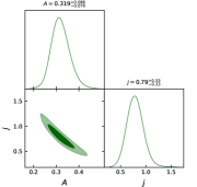
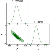
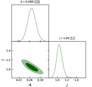
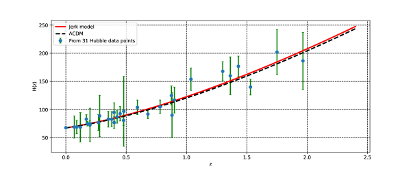
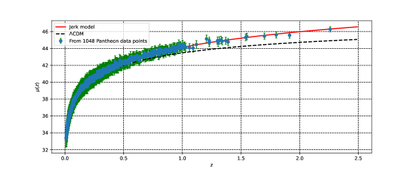
respectively. The model parameter constraints are derived by minimizing the corresponding $\chi^{2}$ using MCMC and the emcee library (Tab. 1 shows the results). During our MCMC analysis, we employed a total of 100 walkers and executed 1000 steps to obtain our results. Fig. 1 shows the $1-\sigma$ and $2-\sigma$ likelihood curves for the model parameters $A$ and $j$ using Hubble, Hubble+SNe, and Hubble+SNe+BAO data sets, respectively. The likelihoods are very well fitted to Gaussian distributions. Moreover, Fig. 1 and Tab. 1 demonstrate that the best fit value of $j$ is really very near to one, which indicates that the model with a constant jerk parameter is temptingly near to the $\Lambda$CDM model. Figs. 2 and 3 also exhibit the error bar fitting for the considered model and the $\Lambda$CDM with $\Omega_{m}^{0}=0.315\pm 0.007$ [3]. The cosmological transition from a decelerating phase to an accelerating phase is widely attributed to the influence of a cosmic jerk. This critical juncture marks a pivotal moment in the universe’s evolution, and its occurrence is closely tied to specific characteristics within different cosmological models. Particularly, this transition is commonly associated with models that exhibit a positive value for the jerk parameter and a concurrent negative value for the deceleration parameter [48, 47]. As a pertinent illustration, consider the $\Lambda$CDM models, which hold a pivotal role in contemporary cosmology. These models are characterized by a constant jerk parameter, specifically $j=1$. This characteristic configuration implies that the $\Lambda$CDM framework undergoes a seamless transition from a decelerating phase to an accelerating phase, marking a turning point in the cosmic trajectory. Based on these findings, it becomes evident that both datasets, specifically the Hubble data and the combined Hubble+SNe datasets, portray a discernible shift in the jerk parameter value from the foundational $\Lambda$CDM model [32]. However, the constraints gleaned from the dataset that combines Hubble, SNe, and BAO (Hubble+SNe+BAO) reveal a comparatively slight deviation from the $\Lambda$CDM model. This observed discrepancy is of such minute magnitude that it can be confidently regarded as negligible. This discernment leads to a compelling conclusion that the model characterized by a constant jerk parameter gravitates tantalizingly close to the $\Lambda$CDM model. The implications of this proximity are noteworthy, as it suggests that the dynamics of the universe, as manifested through the jerk parameter, maintain remarkable similarity to the well-established $\Lambda$CDM framework. Significantly, these findings draw parallels with the outcomes of a study conducted by Mukherjee and Banerjee [49], substantiating the robustness and consistency of our results within the broader cosmological discourse.

(a)

(b)

(c)

Figure 1: Constraints on the model parameters at $1-\sigma$ and $2-\sigma$ confidence interval using the Hubble (a), Hubble+SNe (b), and Hubble+SNe+BAO (c) data sets.

$datasets$	$A$	$j$	$q_{0}$	$z_{tr}$	$\omega_{0}$
$Priors$	$(0,2)$	$(0,2)$	$-$	$-$	$-$
$Hubble$	$0.319_{-0.079}^{+0.086}$	$0.79_{-0.33}^{+0.33}$	$-0.49^{+0.09}_{-0.08}$	$0.76^{+0.37}_{-0.36}$	$-0.92\pm 0.03$
$Hubble+SNe$	$0.292_{-0.049}^{+0.055}$	$0.89_{-0.26}^{+0.26}$	$-0.55^{+0.06}_{-0.05}$	$0.76^{+0.27}_{-0.25}$	$-0.93\pm 0.01$
$Hubble+SNe+BAO$	$0.268_{-0.030}^{+0.032}$	$1.05_{-0.12}^{+0.13}$	$-0.61^{+0.04}_{-0.03}$	$0.73^{+0.15}_{-0.14}$	$-0.94\pm 0.01$

Table 1: The MCMC findings from various datasets have been summarized for a comprehensive overview.

Figure 2: A good fit to the 31 points of the Hubble data sets is displayed in the plot of $H(z)$ versus the redshift $z$ for our $f(Q,T)$ model, which is shown in red, and $\Lambda$CDM, which is shown in black dashed lines.

Figure 3: A good fit to the 1048 points of the Pantheon data sets is displayed in the plot of $\mu(z)$ versus the redshift $z$ for our $f(Q,T)$ model, which is shown in red, and $\Lambda$-CDM, which is shown in black dashed lines.

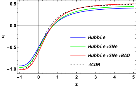
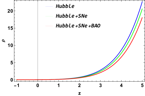
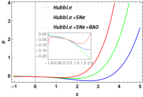
The evolution curves of the DP, pressure and energy density according to the constrained values of the model parameters are shown here. According to Fig. 4, the DP is positive in the early Universe and negative in the late Universe. As a result, it shows that the Universe is transitioning from deceleration to acceleration. The $q$ increases as cosmic red shift increases. The transition redshifts associated to the model parameter values imposed by Hubble, Hubble+SNe, and Hubble+SNe+BAO data sets are estimated as, $z_{tr}=0.76^{+0.37}_{-0.36}$, $0.76^{+0.27}_{-0.25}$, and $z_{tr}=0.73^{+0.15}_{-0.14}$ respectively. Furthermore, the current value of the DP is $q_{0}=-0.49^{+0.09}_{-0.08}$ for the Hubble data sets, $q_{0}=-0.55^{+0.06}_{-0.05}$ for the Hubble+SNe data sets, and $q_{0}=-0.61^{+0.04}_{-0.03}$ for the Hubble+SNe+BAO data sets. In addition, it is essential to point out that the $q_{0}$ and $z_{tr}$ values constrained in this paper are consistent with the values reported in Refs. [56, 57, 58]. The energy density decreases as the Universe expands, as shown in Fig. 5. At late times ($z\rightarrow-1$), the energy density tends to be zero. Fig. 6 further shows that the pressure of the model is negative in the present ($z=0$) and future ($z<0$). Negative pressure is used to describe the process of the acceleration of the Universe in modified gravity. In addition, we discovered that pressure increases with red shift.

Figure 4: The graph above depicts the relationship between the deceleration parameter ($q$) and redshift ($z$) according to the values of model parameters constrained by Hubble, Hubble+SNe, and Hubble+SNe+BAO sets of data.

Figure 5: The graph above depicts the relationship between the energy density ($\rho$) and redshift ($z$) according to the values of model parameters constrained by Hubble, Hubble+SNe, and Hubble+SNe+BAO sets of data.

Figure 6: The graph above depicts the relationship between the pressure ($p$) and redshift ($z$) according to the values of model parameters constrained by Hubble, Hubble+SNe, and Hubble+SNe+BAO data sets.

V EoS parameter $\omega$ and energy conditions

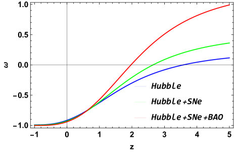
The effective or total equation of state (EoS) $\omega$ is determined by dividing the total pressure by the total energy density, i.e. $\omega=\frac{p}{\rho}$. The evolution of the energy density and the expansion of the universe are directly intertwined with the behavior of this parameter. Different EoS values correlate to distinct epochs of the Universe in its early decelerating and current accelerating expanding stages. It contains stiff-fluid, radiation, and matter dominated (dust) for $\omega=1$, $\omega=\frac{1}{3}$, and $\omega=0$ (decelerating stages), respectively. It depicts quintessence $-1<\omega<-\frac{1}{3}$, the cosmological constant $\omega=-1$, and the phantom scenario, $\omega<-1$. By using Eqs. (20) and (21) we get the expression for EoS parameter and plot its behavior in Fig. 7 for the parameter values of the model constrained from three data sets. Fig. 7 shows that $\omega$ is presently negative and exhibiting quintessence dark energy, indicating an accelerating phase. It should be noticed that the EoS parameter in our model tends to $-1$ at late periods. As a result, it behaves as a cosmological constant at late periods. Also, the current values of the EoS parameter for the Hubble, Hubble+SNe, and Hubble+SNe+BAO data sets are $\omega_{0}=-0.92\pm 0.03$, $\omega_{0}=-0.93\pm 0.01$, and $\omega_{0}=-0.94\pm 0.01$, respectively [59, 60].

Figure 7: The graph above depicts the relationship between the EoS parameter ($\omega$) and redshift ($z$) according to the values of model parameters constrained by Hubble, Hubble+SNe, and Hubble+SNe+BAO sets of data.

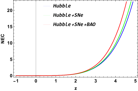
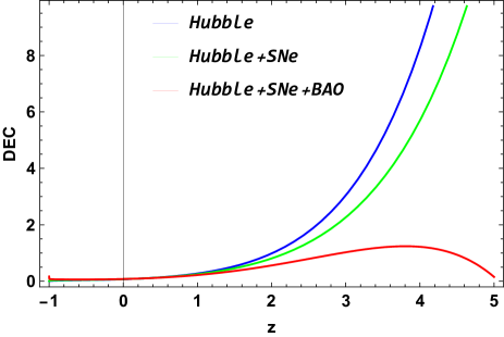
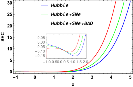
We know that physical parameters such as DP and EoS parameter are important in the study of the Universe. Another major research in current cosmology is on energy conditions derived from Raychaudhuri’s equation. The main objective of these energy conditions is to limit the expansion of the Universe. Energy conditions include null energy condition (NEC), weak energy condition (WEC), dominant energy condition (DEC), and strong energy condition (SEC) (SEC). These energy conditions are described in $f(Q,T)$ modified theory of gravity with specified energy density $\rho$ and pressure $p$ as follows: $\rho+p\geq 0$ and $\rho\geq 0$ (WEC); $\rho+p\geq 0$ (NEC); $\rho\geq\left|p\right|$ and $\rho\geq 0$ (DEC); $\rho+3p\geq 0$ (SEC). The violation of NEC leads in the violation of leftover energy conditions (also the violation of the NEC results in the violation of the second law of thermodynamics), it reflects the depletion of energy density with the expanding Universe. Further, the violation of SEC indicates the acceleration of the Universe [61].

Figure 8: The graph above depicts the relationship between the NEC condition and redshift ($z$) according to the values of model parameters constrained by Hubble, Hubble+SNe, and Hubble+SNe+BAO data sets.

Figure 9: The graph above depicts the relationship between the DEC condition and redshift ($z$) according to the values of model parameters constrained by Hubble, Hubble+SNe, and Hubble+SNe+BAO data sets.

Figure 10: The graph above depicts the relationship between the SEC condition and redshift ($z$) according to the values of model parameters constrained by Hubble, Hubble+SNe, and Hubble+SNe+BAO data sets.

Figs. 8, 9, and 10 depict graphs of energy conditions with regard to redshift, and we can see from these figures that NEC and DEC are currently satisfied. Also, as seen in Fig. 10, $\rho+3p\leq 0$ results in a violation of the SEC at the present. Thus, violating SEC causes the Universe to accelerate.

VI $Om(z)$ diagnostic

The $Om(z)$ diagnostic serves as a valuable tool for scrutinizing distinctions between the conventional $\Lambda$CDM model and alternative DE models. This diagnostic method proves to be more user-friendly than the statefinder diagnosis [6], given its reliance solely on the primary temporal derivative of the cosmic scale factor. This streamlined approach is attributed to its dependence solely on the Hubble parameter, which in turn relies on a solitary time derivative of $a(t)$, the cosmic scale factor. In the context of a spatially flat universe, the definition of the $Om(z)$ diagnostic takes the form:

$$Om\left(z\right)=\frac{h^{2}(z)-1}{\left(1+z\right)^{3}-1}.$$ (37)

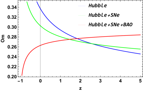
Alternatively, we can express that the $Om(z)$ diagnostic provides us with a null test for evaluating the cosmological constant. In the scenario where DE corresponds to a cosmological constant, the behavior of $Om(z)$ becomes linear with a constant slope, specifically $Om(z)=\Omega_{m}^{0}$. However, for alternative DE models, $Om(z)$ takes on a curved trajectory. Specifically, a negative slope within the $Om(z)$ curve indicates quintessence-like behavior, while a positive slope corresponds to a phantom-like behavior. As depicted in Fig. 11, the $Om(z)$ diagnostic, constrained by the limited values of the model parameters extracted from the Hubble and Hubble+SNe datasets, exhibits a consistent negative slope across the cosmic evolution. In this context, the jerk model is indicative of quintessence-like behavior. Conversely, when considering the Hubble+SNe+BAO datasets, the $Om(z)$ diagnostic demonstrates a positive slope, corresponding to a phantom-like behavior of the Universe within this framework.

Figure 11: The graph above depicts the relationship between the $Om\left(z\right)$ parameter and redshift ($z$) according to the values of model parameters constrained by Hubble, Hubble+SNe, and Hubble+SNe+BAO sets of data.

VII Concluding remarks

The paper describes the phenomenon of late-time acceleration in the context of $f(Q,T)$ gravity, which is constructed from an arbitrary function of non-metricity scalar non-minimally coupled to the trace of the stress-energy tensor. We have investigated the functional form $f(Q,T)=f\left(Q\right)+f\left(T\right)$, where $f\left(Q\right)=Q+\alpha\,Q^{2}$ is the Starobinsky model in $f\left(Q\right)$ gravity and $f\left(T\right)=2\,\gamma\,T$, where $\alpha$ and $\gamma$ are constants. We considered a constant jerk to get accurate solutions to the field equations, and then we used the definition of this jerk to determine the evolution of the other kinematical variables such as the deceleration parameter, the energy density, EoS parameter, and different energy conditions to validate the proposed model.

In Sec. IV, to constrain the model parameters $A$ and $j$, we analyzed the most available Pantheon SNe set of data collection with 1048 points, the Hubble set of data with 31 points, and the BAO set of data with six points. For the Hubble data sets, the combined Hubble+SNe sets of data and the combined Hubble+SNe+BAO data sets, we estimated the best fit values of the model parameters $A$ and $j$. The results obtained are summarized in Fig. 1 and Tab. 1. Thus, the obtained data clearly indicate that the best fit value of $j$, which has been chosen as a constant in this study, is extremely near to one i.e. $j\sim 1$, which is compatible with a $\Lambda$CDM model. Current findings on constant jerk parametrization show that a $\Lambda$CDM is clearly recommended [62, 40]. We also examined the evolution of various cosmological parameters corresponding to the best fit values of the model parameters. The deceleration parameter is positive in the early Universe and negative in the late Universe. Thus, it shows that the Universe is transitioning from deceleration to acceleration. The transition red shifts associated to the model parameter values imposed by Hubble, Hubble+SNe, and Hubble+SNe+BAO data sets are estimated as $z_{tr}=0.76^{+0.37}_{-0.36}$, $z_{tr}=0.76^{+0.27}_{-0.25}$, and $z_{tr}=0.73^{+0.15}_{-0.14}$ respectively. Further, the current values of the DP are $q_{0}=-0.49^{+0.09}_{-0.08}$ for the Hubble data sets, $q_{0}=-0.55^{+0.06}_{-0.05}$ for the Hubble+SNe data sets, and $q_{0}=-0.61^{+0.04}_{-0.03}$ for the Hubble+SNe+BAO sets of data. The energy density decreases as the Universe expands. So, the negative pressure is a term used to explain the process of the acceleration of the Universe in modified gravity.

In Sec. V, we discussed the EoS parameter, and different energy conditions to validate the proposed model. It is observed that the EoS parameter in our model tends to $-1$ ($\Lambda$CDM model) in the late time evolution. Further, the current values of the EoS parameter for the Hubble, Hubble+SNe, and Hubble+SNe+BAO data sets are $\omega_{0}=-0.92\pm 0.03$, $\omega_{0}=-0.93\pm 0.01$, and $\omega_{0}=-0.94\pm 0.01$, respectively. The NEC and DEC conditions are currently satisfied, while the SEC at the present. Thus, violating SEC causes the Universe to accelerate.

Finally, in Sec. VI, the Om diagnostics are examined in order to differentiate between various dark energy theories. It is noted that the $Om\left(z\right)$ diagnostic parameter for the Hubble and Hubble+SNe sets of data has a negative slope throughout of the Universe. Thus, the jerk model represents quintessence type behavior. Also, for the Hubble+SNe+BAO data sets the $Om\left(z\right)$ has a positive slope. Thus, it represents the phantom type behavior of the Universe. As a consequence, the research shows that the constant jerk parameter in $f(Q,T)$ Starobinsky gravity may be employed to generate cosmic acceleration.

Data Availability

All generated data are included in this manuscript.

References

- [1] A.G. Riess et al., Observational evidence from supernovae for an accelerating universe and a cosmological constant, Astron. J. 116 (1998) 1009-1038, http://dx.doi.org/10.1086/300499.
- [2] S. Perlmutter et al., Measurements of and from 42 high-redshift supernovae, Astrophys. J. 517 (1999) 565-586, http://dx.doi.org/10.1086/307221.
- [3] N. Aghanim et al., Planck 2018 results-VI. Cosmological parameters, Astron. Astrophys. 641 (2020) A6, https://doi.org/10.1051/0004-6361/201833910.
- [4] S. Weinberg, The cosmological constant problem, Rev. Mod. Phys. 61 (1989) 1, https://doi.org/10.1103/RevModPhys.61.1.
- [5] A. Y. Kamenshchik et al., An alternative to quintessence, Phys. Lett. B. 511 (2001) 265-268, https://doi.org/10.1016/S0370-2693(01)00571-8.
- [6] V. Sahni and Y. Shtanov, Braneworld models of dark energy, J. Cosmol. Astropart. Phys.. 11 (2003) 014, https://doi.org/10.1088/1475-7516/2003/11/014.
- [7] M. Li, A model of holographic dark energy, Phys. Lett. B. 603 (2004) 1-5, https://doi.org/10.1016/j.physletb.2004.10.014.
- [8] R. G. Cai, A dark energy model characterized by the age of the universe, Phys. Lett. B. 657 (2007) 228-231, https://doi.org/10.1016/j.physletb.2007.09.061.
- [9] T. Padmanabhan, Accelerated expansion of the universe driven by tachyonic matter, Phys. Rev. D. 66 (2002) 02131, https://doi.org/10.1103/PhysRevD.66.021301.
- [10] R. R. Caldwell, A phantom menace? Cosmological consequences of a dark energy component with super-negative equation of state, Phys. Lett. B 545 (2002) 23-29, https://doi.org/10.1016/S0370-2693(02)02589-3.
- [11] S. Nojiri and S. D. Odintsov, Quantum de Sitter cosmology and phantom matter, Phys. Lett. B 562 (2003) 147-152, https://doi.org/10.1016/S0370-2693(03)00594-X.
- [12] H.A. Buchdahl, Non-linear Lagrangians and cosmological theory, Month. Not. R. Astron. Soc., 150 (1970) 1, https://doi.org/10.1093/mnras/150.1.1.
- [13] S. Capozziello, V. F. Cardone, V. Salzano, Cosmography of f(R) gravity, Phys. Rev. D, 78 (2008) 063504-063521, http://dx.doi.org/10.1103/PhysRevD.78. 063504.
- [14] S. Capozziello et al., Cosmography in f(T) gravity, Phys. Rev. D, 84 (2011) 043527, https://doi.org/10.1103/PhysRevD.84.043527.
- [15] Di Liu, M. J. Reboucas, Energy conditions bounds on f(T) gravity, Phys. Rev. D, 86 (2012) 083515, https://doi.org/10.1103/PhysRevD.86.083515.
- [16] T. Harko, et al., f (R, T) gravity, Phys. Rev. D 84 (2011) 024020, https://doi.org/10.1103/PhysRevD.84.024020.
- [17] J. B. Jimenez, L. Heisenberg, T. Koivisto, Coincident general relativity, Phys. Rev. D, 98 (2018) 044048-044054, http://dx.doi.org/10.1103/PhysRevD.98. 044048.
- [18] Y. Xu et al., f(Q,T) Gravity, Eur. Phys. J. C 79 (2019) 708, http://dx.doi.org/10.1140/epjc/s10052-019-7207-4.
- [19] J.M. Nester and H.J. Yo, Symmetric teleparallel general relativity, Chin. J. Phys. 37 (1999) 113, https://doi.org/10.48550/arXiv.gr-qc/9809049.
- [20] R. Zia, D. C. Maurya, and A. K. Shukla, Transit cosmological models in modified f (Q, T) gravity, Int. J. Geom. Methods Mod. Phys. 18 (2021) 2150051, https://doi.org/10.1142/S0219887821500511.
- [21] N. Godani, G. C. Samanta, FRW cosmology in f(Q,T) gravity, Int. J. Geom. Methods Mod. Phys, 18 (2021) 2150134, https://doi.org/10.1142/S0219887821501346.
- [22] S. Bhattacharjee and P. K. Sahoo, Baryogenesis in f(Q,T) gravity, Eur. Phys. J. C 80, (2020) 289, http://dx.doi.org/10.1140/epjc/s10052-020-7844-7.
- [23] K. El Bourakadi et al., Constant-roll and primordial black holes in f (Q, T) gravity, Phys. Dark Universe41 (2023) 101246, https://doi.org/10.1016/j.dark.2023.101246.
- [24] M. Tayde et al., Static spherically symmetric wormholes in gravity, Chin. Phys. C46 (2022) 115101, https://doi.org/10.1088/1674-1137/ac7f22.
- [25] A. Najera and A. Fajardo, Cosmological perturbation theory in f(Q,T) gravity, J. Cosmol. Astropart. Phys.03 (2022) 020, https://doi.org/10.1088/1475-7516/2022/03/020.
- [26] S. Arora and P.K. Sahoo, Energy conditions in f (Q, T) gravity, Phys. Scr.95 (2020) 095003, https://doi.org/10.1088/1402-4896/abaddc.
- [27] S. Arora et al., f(Q,T) Gravity models with observational constraints, Phys. Dark Univ. 30 (2020) 100664-100671, http://dx.doi.org/10.1016/j.dark. 2020.100664.
- [28] A.S. Agrawal et al., Matter bounce scenario in extended symmetric teleparallel gravity, Eur. Phys. J. C83 (2021) 113, https://doi.org/10.1140/epjc/s10052-023-11266-8.
- [29] A. Pradhan, G. Goswami, and A. Beesham, The reconstruction of constant jerk parameter with f(R,T) gravity,J. High Energy Phys.38 (2023) 12-21, https://doi.org/10.1016/j.jheap.2023.03.001.
- [30] R. D. Blandford et al., Observing Dark Energy, 339 (2005) 27, https://doi.org/10.48550/arXiv.astro-ph/0408279.
- [31] D. Rapetti, S.W. Allen, M.A. Amin, R.D. Blandford, A kinematical approach to dark energy studies, Mon. Not. R. Astron. Soc., 375 (2007) 1510, https://doi.org/10.1111/j.1365-2966.2006.11419.x.
- [32] Z. X. Zhai et al., Reconstruction and constraining of the jerk parameter from OHD and SNe Ia observations, Phys. Lett. B, 727 (2013) 8-20, https://doi.org/10.1016/j.physletb.2013.10.020.
- [33] S. K. J. Pacif, Dark energy models from a parametrization of H: a comprehensive analysis and observational constraints, Eur. Phys. J. Plus, 135 (2020) 10, https://doi.org/10.1140/epjp/s13360-020-00769-y.
- [34] S. K. J. Pacif, R. Myrzakulov, S. Myrzakul, Reconstruction of cosmic history from a simple parametrization of H, Int. J. Geom. Methods Mod., 14 (2017) 07, https://doi.org/10.1142/S0219887817501110.
- [35] M. Koussour et al., A New Parametrization of Hubble Parameter in f(Q) Gravity, Fortschr. Phys., 71 (2023) 2200172, https://doi.org/10.1002/prop.202200172.
- [36] S. Del Campo et al., Three thermodynamically based parametrizations of the deceleration parameter, Phys. Rev. D 86 (2012) 083509, https://doi.org/10.1103/PhysRevD.86.083509.
- [37] A. Mukherjee and N. Banerjee, A reconstruction of quintessence dark energy, Eur. Phys. J. Plus 130 (2015) 1-8, https://doi.org/10.1140/epjp/i2015-15201-7.
- [38] R. Jimenez, A. Loeb, Constraining cosmological parameters based on relative galaxy ages, Astrophys. J. 573 (2002) 37, https://doi.org/10.1086/340549.
- [39] P. Mukherjee, N. Banerjee, Non-parametric reconstruction of the cosmological jerk parameter, Eur. Phys. J. C, 81 (2021) 36, https://doi.org/10.1140/epjc/s10052-021-08830-5.
- [40] P. Mukherjee, N. Banerjee, Parametric reconstruction of the cosmological jerk from diverse observational data sets, Phys. Rev. D, 93 (2016) 043002, https://doi.org/10.1103/PhysRevD.93.043002.
- [41] A. Gomez-Valent, Luca Amendola, H0 from cosmic chronometers and Type Ia supernovae, with Gaussian Processes and the novel Weighted Polynomial Regression method, J. Cosmol. Astropart. Phys. 04 (2018) 051, https://doi.org/10.1088/1475-7516/2018/04/051.
- [42] G. S. Sharov and V. O. Vasilie, How predictions of cosmological models depend on Hubble parameter data sets, Mathematical Modelling and Geometry 6 (2018) 1-20, https://doi.org/10.26456/mmg/2018-611.
- [43] D. M. Scolnic et al., The complete light-curve sample of spectroscopically confirmed SNe Ia from Pan-STARRS1 and cosmological constraints from the combined pantheon sample, Astrophys. J. 859 (2018) 101, https://doi.org/10.3847/1538-4357/aab9bb.
- [44] C. Blake et al., The WiggleZ Dark Energy Survey: mapping the distance-redshift relation with baryon acoustic oscillations, Mon. Not. Roy. Astron. Soc. 418 (2011) 1707-1724, https://doi.org/10.1111/j.1365-2966.2011.19592.x.
- [45] W. J. Percival et al., Baryon acoustic oscillations in the Sloan Digital Sky Survey data release 7 galaxy sample, Mon. Not. Roy. Astron. Soc. 401 (2010) 2148-2168, https://doi.org/10.1111/j.1365-2966.2009.15812.x.
- [46] R. Giostri et al., From cosmic deceleration to acceleration: new constraints from SN Ia and BAO/CMB, J. Cosm. Astropart. Phys. 03 (2012) 027, https://doi.org/10.1088/1475-7516/2012/03/027.
- [47] M. Visser, Jerk, snap and the cosmological equation of state, Class. Quantum Gravity 21 (2004) 2603, https://doi.org/10.1088/0264-9381/21/11/006.
- [48] T. Chiba and T. Nakamura, The luminosity distance, the equation of state, and the geometry of the universe, Prog. Theor. Phys. 100 (1998) 1077-1082, https://doi.org/10.1143/PTP.100.1077.
- [49] A. Mukherjee and N. Banerjee, In search of the dark matter dark energy interaction: a kinematic approach, Class. Quantum Gravity 34 (2017) 035016, https://doi.org/10.1088/1361-6382/aa54c8.
- [50] A. A. Starobinsky, A new type of isotropic cosmological models without singularity, Phys. Lett. B 91 99-102 (1980), https://doi.org/10.1016/0370-2693(80)90670-X.
- [51] A. A. Starobinsky, Disappearing cosmological constant in f(R) gravity, JETP Letters 86 (2007) 157-163, https://doi.org/10.1134/S0021364007150027.
- [52] M. Sharif and A. Siddiqa, Axial dissipative dust as a source of gravitational radiation in f (R) gravity, Phys. Dark Universe 15, 105-113 (2017), https://doi.org/10.1016/j.dark.2017.01.004.
- [53] D. F. Mackey et al., emcee: the MCMC hammer, Publ. Astron. Soc. Pac. 125 (2013) 306, https://doi.org/10.1086/670067.
- [54] R. Kessler and D. Scolnic, Correcting type Ia supernova distances for selection biases and contamination in photometrically identified samples, Astrophys. J. 836 (2017) 56, https://doi.org/10.3847/1538-4357/836/1/56.
- [55] A. Raychaudhuri, Relativistic cosmology. I, Phys. Rev. 98 (1955) 1123, https://doi.org/10.1103/PhysRev.98.1123.
- [56] S. Capozziello, R. D Agostino and O. Luongo, High-redshift cosmography: auxiliary variables versus Padé polynomials S Capozziello, R D’Agostino, O Luongo,Mon. Not. Roy. Astron. Soc. 494 (2020) 2576-2590, https://doi.org/10.1093/mnras/staa871.
- [57] S. A. Al Mamon and S. Das, A parametric reconstruction of the deceleration parameter, Eur. Phys. J. C 77 (2017) 495, https://doi.org/10.1140/epjc/s10052-017-5066-4.
- [58] S. Basilakos, F. Bauera and J. Sola, Confronting the relaxation mechanism for a large cosmological constant with observations,J. Cosmol. Astropart. Phys. 2012 (2012) 050, https://doi.org/10.1088/1475-7516/2012/01/050.
- [59] A. Hernandez-Almada, et al., Cosmological constraints on alternative model to Chaplygin fluid revisited, Eur. Phys. J. C 79 (2019) 1-2, https://doi.org/10.1140/epjc/s10052-018-6521-6.
- [60] Q. J. Zhang and Y. L. Wu, Dark Energy and Hubble Constant From the Latest SNe Ia, BAO and SGL ,J. Cosmol. Astropart. Phys. 2010 (2010) 08, https://doi.org/10.48550/arXiv.0905.1234.
- [61] M. Visser and C Barcelo, Energy conditions and their cosmological implications, COSMO-99 (2000) 98, https://doi.org/10.1142/9789812792129-0014.
- [62] Z.-X. Zhai et al., Reconstruction and constraining of the jerk parameter from OHD and SNe Ia observations, Phys. Lett. B 727 (2013) 8-20, https://doi.org/10.1016/j.physletb.2013.10.020.