Precision Rydberg State Spectroscopy with Slow Electrons and Proton Radius Puzzle

Abstract

The so-called proton radius puzzle (the current discrepancy of proton radii determined from spectroscopic measurements in ordinary versus muonic hydrogen) could be addressed via an accurate measurement of the Rydberg constant, because the proton radius and the Rydberg constant values are linked through high-precision optical spectroscopy. We argue that, with manageable additional experimental effort, it might be possible to improve circular Rydberg state spectroscopy, potentially leading to an important contribution to the clarification of the puzzle. Our proposal involves circular and near-circular Rydberg states of hydrogen with principal quantum number around $n=18$, whose classical velocity on a Bohr orbit is slower than that of the fastest macroscopic man-made object, the Parker Solar Probe. We obtain improved estimates for the quality factor of pertinent transitions, and illustrate a few recent improvements in instrumentation which facilitate pertinent experiments.

I Introduction

The Rydberg constant is of consummate importance for our understanding of fundamental physics. Notably, this constant is an important input datum for the calculation of transition frequencies in hydrogen and deuterium (see Table II of Ref. Jentschura et al. (2005) and Refs. Mohr et al. (2008); Tiesinga et al. (2021)). In addition to the Rydberg constant, accurate values of the proton and deuteron radii are also required in order to calculate transition frequencies in hydrogen and deuterium. Conversely, one can infer proton and deuteron radii from precise values of hydrogen and deuterium frequencies (see Refs. Jentschura et al. (2005); Tiesinga et al. (2021) and Table 45 of Ref. Mohr et al. (2008)).

With the advent of muonic hydrogen spectroscopic measurements Pohl et al. (2010, 2016), the CODATA value of the proton radius has shifted from a 2006 value of about $R_{p}\approx 0.88\,{\rm fm}$ to a 2018 value of about $R_{p}\approx 0.84\,{\rm fm}$, entailing a concomitant change in the Rydberg constant Mohr et al. (2008); Tiesinga et al. (2021). From the 2006 to the 2018 CODATA adjustments Mohr et al. (2008); Tiesinga et al. (2021), the Rydberg constant has shifted by much more than the uncertainty associated with the 2006 value (see Fig. 1).

One of the most attractive experimental pathways to the determination of the Rydberg constant involves highly excited Rydberg states in atomic hydrogen, as described in Ref. Lutwak et al. (1997) by a research group working at the Massachusetts Institute of Technology (MIT). Within the same group, a value for the Rydberg constant was obtained in an unpublished thesis by de Vries deVries (labelled as “Rydberg state” in Fig. 1),

$$\left.cR_{\infty}\right|_{\mathrm{deVries}}=3\,289\,841\,960\,306(69)\,{\rm kHz}\,,$$ (1)

which is consistent with the CODATA 2006 value, and barely consistent with the 2018 CODATA value from Ref. Tiesinga et al. (2021):

$$\left.cR_{\infty}\right|_{\rm CODATA,2018}=3\,289\,841\,960\,250(7)\,{\rm kHz}\,.$$ (2)

The 2006 CODATA value is discrepant,

$$\left.cR_{\infty}\right|_{\rm CODATA,2006}=3\,289\,841\,960\,360(21)\,{\rm kHz}\,.$$ (3)

A comparison of the three values of the Rydberg constant is made in Fig. 1, where we use as the reference value

$$R_{0}=\left.R_{\infty}\right|_{\rm CODATA,2018}\,.$$ (4)

Figure 1: We examine the values for the Rydberg constant, converted to frequency units, from CODATA adjustments and from the (unpublished, grayed) result communicated in Ref. deVries . The CODATA (2006) value was reported in Ref. Mohr et al. (2008), and the CODATA (2018) value is from Ref. Tiesinga et al. (2021). The reference value $R_{0}$ is from the 2018 adjustment.

The situation is interesting because, before the advent of muonic hydrogen spectroscopy, values of the Rydberg constant and of the proton radius inferred from hydrogen and deuterium spectroscopy alone (without any additional input from scattering experiments) were consistent with the 2006 CODATA values for both the 2006 CODATA value of the Rydberg constant, as well as the 2006 CODATA values of the proton and deuteron radii. This is discussed in detail in the discussion surrounding Table 45 of Ref. Mohr et al. (2008), where it is pointed out that the proton radius $R_{p}$, the deuteron radius $R_{d}$, and the Rydberg constant can all be deduced using input data exclusively from hydrogen and deuterium spectroscopy.

Traditionally, the Rydberg constant has been determined on the basis of Rydberg-state spectroscopy of atomic hydrogen Kibble et al. (1973); Gallagher (1994); Biraben et al. (1989); Nez et al. (1992); de Beauvoir et al. (1997); Schwob et al. (1999); de Beauvoir et al. (2000). An improved measurement of the Rydberg constant would thus constitute an important contribution to a resolution of the proton radius puzzle Jentschura (2022). In a remarkable investigation dating about 20 years back, circular Rydberg states around quantum numbers $n\approx 30$ have been investigated with the ultimate aim of an improved measurement of the Rydberg constant deVries . Inspired by the importance of Rydberg states, it has been pointed out in Refs. Jentschura et al. (2008, 2009, 2010) that Rydberg-state measurements in hydrogenlike ions of medium charge numbers could potentially offer an alternative route to a determination of the Rydberg constant.

The purpose of this paper is threefold. First, we update the calculation of the quality factors for transitions among circular Rydberg states, in comparison to the estimate provided in Eq. (6) of Ref. Jentschura et al. (2008). Second, we discuss the status of quantum electrodynamic theory of Rydberg states, demonstrate that the theory is very well under control on the level of accuracy required for a determination of the Rydberg constant on the level of precision required for a resolution of the proton radius puzzle, and discuss the relative suppression of a number of notoriously problematic quantum electrodynamic corrections for circular and near-circular Rydberg states. Calculated values for relativistic Bethe logarithms for circular and near-circular Rydberg states with principal quantum numbers $16\leq n\leq 20$ are also provided. Third, we provide an overview of recent advances in laser technology and other experimental techniques, which facilitate an improvement of measurements of the Rydberg constant on the basis of Rydberg state measurements. SI mksA units are employed throughout this paper.

II Quality Factors

Of crucial importance for the feasibility of high-precision spectroscopy experiments are so-called quality factors of transitions. The quality factor is the dimensionless ratio of the transition energy to the natural line width of the transition (measured in radians per second), where the latter is converted to an energy via multiplication by the reduced Planck constant $\hbar$. Here, we present the general formula for the one-photon decay rate of a circular Rydberg state, with principal quantum number $n$ and maximum orbital angular moment $\ell=n-1$. This reference state can decay, due to dipole transitions to states with principal quantum number $n-1$ and angular momentum quantum number $\ell=n-2$. For the decay rate of the state with principal quantum number $n$ and maximum orbital angular moment $\ell=n-1$, as parameterized by the imaginary part of the self energy, $E={\rm Re}\,E-\mathrm{i}\Gamma_{n}/2$, we find the result

$$\Gamma^{\ell=n-1}_{n}=\frac{4^{2n}(n-1)^{2n-1}\,n^{2n-4}}{(2n-1)^{4n-1}(2n-3)}\,\frac{\alpha(Z\alpha)^{4}m\,c^{2}}{3n^{5}}\,\left(\frac{\mu}{m}\right)^{3}$$ (5)

which can be expanded for large $n$ as follows,

$$\Gamma^{\ell=n-1}_{n}=\alpha\frac{(Z\alpha)^{4}mc^{2}}{3n^{5}}\,\left(\frac{\mu}{m}\right)^{3}\\ \times\left[1+\frac{3}{2n}+\frac{17}{8n^{2}}+\mathcal{O}\left(\frac{1}{n^{3}}\right)\right]\,,$$ (6)

where $m$ is the electron mass, $\mu$ is the reduced mass of the two-body system, $\alpha$ is the fine-structure constant, $Z$ is the nuclear charge number, and the expansion for large $n$ illustrates that the lifetimes of circular Rydberg states scale as $n^{5}$. The energy difference for transitions among circular Rydberg states is

$$E_{n}-E_{n-1}=\frac{(Z\alpha)^{2}\mu}{2}\,\left(\frac{1}{(n-1)^{2}}-\frac{1}{n^{2}}\right)\,,$$ (7)

which scales as $1/n^{3}$ for large $n$. Due to the $1/n^{5}$ asymptotics of the decay rate and the $1/n^{3}$ asymptotics of the transition energy, the quality factor increases, for large $n$, with the square of the principal quantum number $n$,

$$Q=\frac{E_{n}-E_{n-1}}{\Gamma^{\ell=n-1}_{n}+\Gamma^{\ell=n-2}_{n-1}}\\ =\frac{3n^{2}}{2\alpha\,(Z\alpha)^{2}}\,\left(\frac{m}{\mu}\right)^{2}\,\left[1-\frac{5}{2n}-\frac{17}{8n^{2}}+\mathcal{O}\left(\frac{1}{n^{3}}\right)\right]\,.$$ (8)

This formula constitutes an update of the estimate given in Eq. (6) of Ref. Jentschura et al. (2008) (the quality factor obtained here is larger by a factor two as compared to Ref. Jentschura et al. (2008)). The estimate in Eq. (8) illustrates the enormous advantages of Rydberg states for the measurement of the Rydberg constant. The dramatic increase of the quality factor with the square of the principal quantum number makes Rydberg state transitions very attractive. Also, we observe that the quality factor is inversely proportional to the second power of the nuclear charge number $Z$. This means that $Z=1$ (atomic hydrogen) offers the best quality factor, for given principal quantum number $n$.

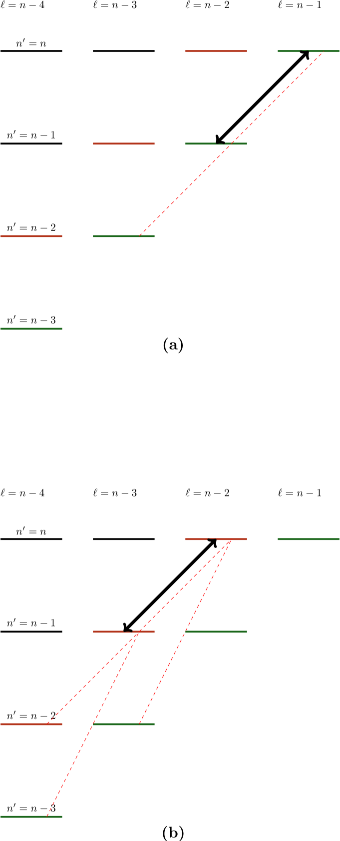
Figure 2: The level diagram for Rydberg states illustrates the dipole-allowed transitions among circular [panel (a)] and near-circular [panel (b)] states. Transitions driven for high-precision spectroscopy are indicated with two-sided arrows. Transitions relevant for the calculation of decay rates (quality factors) are indicated by dashed lines. Circular Rydberg levels with $\ell=n-1$ are marked in green color, while near-circular Rydberg levels with $\ell=n-2$ are marked in red color.

Let us also evaluate the quality factor for the transition among near-circular Rydberg states, where the upper level has orbital angular momentum $\ell=n-2$ and the lower level has orbital angular $\ell=n-3$ (see also Fig. 2). The calculation of the quality factor proceeds in a similar way, but one needs to consider two available dipole decay channels, namely, from the reference state with principal quantum number $n$ and orbital angular momentum quantum number $\ell=n-2$, to lower states with $n^{\prime}=n-1$ and $\ell=n-3$, and $n^{\prime}=n-2$ and $\ell=n-3$. The decay width evaluates to

$$\Gamma^{\ell=n-2}_{n}=\alpha\frac{(Z\alpha)^{4}mc^{2}}{3n^{5}}\,\left(\frac{\mu}{m}\right)^{3}\\ \times\left[1-\frac{1}{2n}-\frac{1}{8n^{2}}+\mathcal{O}\left(\frac{1}{n^{3}}\right)\right]\\ +\alpha\frac{4(Z\alpha)^{4}mc^{2}}{3n^{6}}\,\left(\frac{\mu}{m}\right)^{3}\\ \times\left[1+\frac{5}{2n}+\frac{25}{4n^{2}}+\mathcal{O}\left(\frac{1}{n^{3}}\right)\right]\,,$$ (9)

where the two terms on the right-hand side correspond to the lower states with $n^{\prime}=n-1$ and $n^{\prime}=n-2$, respectively. The quality factor evaluates to

$$Q^{\prime}=\frac{E_{n}-E_{n-1}}{\Gamma^{\ell=n-2}_{n}+\Gamma^{\ell=n-3}_{n-1}}\\ =\frac{3n^{2}}{2\alpha\,(Z\alpha)^{2}}\left(\frac{m}{\mu}\right)^{2}\,\left[1-\frac{9}{2n}+\frac{9}{8n^{2}}+\mathcal{O}\left(\frac{1}{n^{3}}\right)\right]\,,$$ (10)

which is commensurate with $Q$ given in Eq. (8) and illustrates that no significant accuracy loss occurs if one measures near-circular as opposed to circular Rydberg states.

A quick look at Eqs. (1), (2) and (3), and Fig. 1, illustrates that one needs to resolve the Rydberg constant to roughly one part in $10^{11}$ or better in order to meaningfully distinguish between the 2006 and 2018 CODATA values of the Rydberg constant. One can convert this resolution to a splitting factor $\mathcal{S}$, which measures the fraction to which one needs to split the resonance line in order to achieve a resolution of one one part in $10^{11}$. The splitting factor $\mathcal{S}$ is given by the formula

$$\mathcal{S}=10^{11}/Q\,.$$ (11)

For $Z=1$, one obtains for $\mathcal{S}$ the perfectly reasonable figure $\mathcal{S}=93$ for $n=18$; expressed differently, one only needs to split the resonance lines near $n=18$ to one part in 93 is order to achieve a resolution which meaningfully contributes to a resolution of the proton radius puzzle.

Cross-damping terms (non-resonant corrections) can be generated by virtual levels displaced by a fine-structure interval Jentschura and Mohr (2002). A rough estimate of the corresponding energy (frequency) shift $\delta E_{\rm CD}$ (we set $\hbar=1$) is given by the expression Jentschura and Mohr (2002)

$$\delta E_{\rm CD}\sim\frac{\Gamma_{n}^{2}}{\delta E}\,,$$ (12)

Here, $\delta E$ is the displacement of the virtual state responsible for the cross-damping energy shift. As pointed out in Ref. Jentschura and Mohr (2002), the nearest virtual states which can contribute to differential cross sections are states displaced from the upper state of the Rydberg transition by a fine-structure interval. The maximum angular momentum is $\ell_{\rm max}=n-1$. The total angular momenta for the circular Rydberg states are $\ell_{\rm max}\pm 1/2$. The two possible values for the total angular momentum quantum numbers of the upper level are thus $j_{+}=n-1/2$ and $j_{-}=n-3/2$, one of these being the reference level, the other being the virtual level which contributes to the cross damping. So, we have potential nonresonant contributions from virtual levels with an energy displacement

$$\delta E=E_{n,j_{+}}-E_{n,j_{-}}=\frac{(Z\alpha)^{4}m}{2n^{4}(n-1)}\approx\frac{(Z\alpha)^{4}m}{2n^{5}}\,.$$ (13)

The ratio of the cross-damping energy shifts relative to transition frequency is thus estimated by the expression

$$\chi\equiv\frac{\delta E_{\rm CD}}{E_{n}-E_{n-1}}\sim\frac{2}{9}\frac{\alpha^{2}(Z\alpha)^{2}}{n^{2}}\,.$$ (14)

For $Z=1$ and $n=18$, this evaluates to $1.9\times 10^{-12}$, which is less than the accuracy required in order to distinguish between the 2006 and 2018 CODATA values of the Rydberg constant. This estimate suggests that cross-damping effects are suppressed for Rydberg states and do not represent an obstacle for the determination of the Rydberg constant from highly excited, circular Rydberg states.

The above estimates given in Eqs. (12)—(14) are valid for the differential cross section Jentschura and Mohr (2002). For the total cross section, these estimates improve even further, consistent with pertinent considerations reported in Refs. Low (1952); Jentschura and Mohr (2002); Udem et al. (2019).

III Quantum Electrodynamic Effects

One might ask if the theory of Rydberg-state transition is well enough under control in order to facilitate the interpretation of a measurement of transitions among Rydberg states. As outlined in Ref. Mohr et al. (2008), the theoretical contributions to the Lamb shift of Rydberg states, on the level necessary for a determination of the Rydberg constant, can be summarized into just four terms: (i) the Dirac energy (in the nonrecoil limit) which is summarized in Eq. (1) of Ref. Jentschura et al. (2008), (ii) the recoil corrections from the Breit Hamiltonian, which are summarized in Eq. (2) of Ref. Jentschura et al. (2008), (iii) the relativistic-recoil corrections summarized in Eq. (3) of Ref. Jentschura et al. (2008), and (iv) the self-energy effect summarized in Eq. (4) of Ref. Jentschura et al. (2008). Calculated values of nonrelativistic Bethe logarithms, which enter the expression for the relativistic recoil correction, have been tabulated for all states with principal quantum numbers $n\leq 200$ in Ref. Jentschura and Mohr (2005). This favorable situation illustrates the tremendous simplifications possible for Rydberg states. Notably, vacuum-polarization, nuclear-size, and nuclear-structure corrections can be completely ignored for circular Rydberg states whose probability density at the nucleus vanishes.

Among the four effects listed above, the most interesting contribution concerns the bound-state self-energy $E_{\rm SE}$, which is described by the formula

$$E_{\rm SE}=\frac{\alpha}{\pi}\frac{(Z\alpha)^{4}\,m}{n^{3}}\,\biggl{(}A_{40}+(Z\alpha)^{2}\\ \times\left\{A_{61}\,\ln\left[\frac{m}{\mu}(Z\alpha)^{-2}\right]+A_{60}\right\}\biggr{)}\,.$$ (15)

The first subscript of the $A$ coefficients counts the number of $Z\alpha$, while the second counts the number of logarithms $\ln[\frac{m}{\mu}(Z\alpha)^{-2}]$.

The general result for the $A_{40}$ coefficient for circular Rydberg states with orbital angular momentum $\ell\neq 0$ and principal quantum number $n\geq 2$ is well known,

$$A_{40}=-\left(\frac{\mu}{m}\right)^{2}\frac{1}{2\kappa(2\ell+1)}\,-\frac{4}{3}\,\left(\frac{\mu}{m}\right)^{3}\ln k_{0}(n,\ell)\,,$$ (16)

where $\kappa=(-1)^{j+\ell+1/2}$ is the Dirac angular quantum number and $\ln k_{0}(n,\ell)$ is the Bethe logarithm. (For values of $\ln k_{0}(n,\ell)$, one consults Ref. Jentschura and Mohr (2005).) The functional dependence on the reduced mass is a consequence of the proton’s convection current; an explanation is given in Chap. 12 of Ref. Jentschura and Adkins (2022). Here, we will place special emphasis on circular, and near-circular Rydberg states with $\ell=n-1$ and $\ell=n-2$, with $n\geq 13$, and refer to them as the following series of states,

• series $\mathcal{A}$: $\ell=n-1$, $j=\ell+1/2$, $\kappa=-(j+1/2)$,

• series $\mathcal{B}$: $\ell=n-1$, $j=\ell-1/2$, $\kappa=(j+1/2)$,

• series $\mathcal{C}$: $\ell=n-2$, $j=\ell+1/2$, $\kappa=-(j+1/2)$,

• series $\mathcal{D}$: $\ell=n-2$, $j=\ell-1/2$, $\kappa=(j+1/2)$.

The $\mathcal{A}$ series has the highest $\ell$ and $j$ for given $n$. The $A_{40}$ coefficients evaluate to the following expressions for the four series of states,

$$\frac{A_{40}(\mathcal{A},n)}{(\mu/m)^{2}}= \;\frac{1}{2n(2n-1)}-\frac{4}{3}\,\frac{\mu}{m}\,\ln k_{0}(n,n-1)$$ (17)

$$\frac{A_{40}(\mathcal{B},n)}{(\mu/m)^{2}}= \;-\frac{1}{2(n-1)(2n-1)}-\frac{4}{3}\,\frac{\mu}{m}\,\ln k_{0}(n,n-1)\,,$$ (18)

$$\frac{A_{40}(\mathcal{C},n)}{(\mu/m)^{2}}= \;\frac{1}{2(n-1)(2n-3)}-\frac{4}{3}\,\frac{\mu}{m}\,\ln k_{0}(n,n-2)\,,$$ (19)

$$\frac{A_{40}(\mathcal{D},n)}{(\mu/m)^{2}}= \;-\frac{1}{2(n-2)(2n-3)}-\frac{4}{3}\frac{\mu}{m}\ln k_{0}(n,n-2)\,.$$ (20)

As a function of the principal quantum number, the Bethe logarithms $\ln k_{0}(n,n-1)$ and $\ln k_{0}(n,n-2)$ decrease with $n$ for large $n$ as $n^{-3}$. In the nonrecoil limit $\mu\to m$, and the limit of large $n$, one has

$$A_{40}(\mathcal{A},n)\approx-A_{40}(\mathcal{B},n)\approx A_{40}(\mathcal{C},n)\\ \approx-A_{40}(\mathcal{D},n)\approx\frac{1}{4n^{2}}\,,\qquad n\to\infty\,.$$ (21)

The leading quantum electrodynamic corrections for circular and near-circular Rydberg states are parameterized by the $A_{40}$ coefficient. The quantum electrodynamic effects are seen to be suppressed, for large $n$, by a factor $n^{-2}$ which appears in addition to the overall scaling factor $n^{-3}$ in Eq. (15).

Higher-loop contributions to the anomalous magnetic moment can be taken into account by the replacement

$$-\left(\frac{\mu}{m}\right)^{2}\frac{1}{2\kappa(2\ell+1)}\to-\left(\frac{\mu}{m}\right)^{2}\frac{1}{2\kappa(2\ell+1)}\frac{a_{e}}{\alpha/(2\pi)}$$ (22)

where $a_{e}$ contains the higher-loop contributions to the electron anomalous magnetic moment, which determines the $g$ factor of the electron according to $g=2(1+a_{e})$. The term $\alpha/(2\pi)$ is the one-loop Schwinger value Schwinger (1948). The quantity $a_{e}$ can either be taken as the most recent experimental value of the electron anomalous magnetic moment Fan et al. (2023), which results in $a_{e}=1.159\,652\,180\,59(13)\times 10^{-3}$, or as a purely theoretical prediction including higher-order effects Laporta (2020).

The suppression of the quantum electrodynamic effects for circular and near-circular Rydberg states has a physical reason: Namely, the velocity of a classical electron orbiting the nucleus in a Bohr orbit corresponding to the principal quantum number $n$ is

$$v_{\rm cl}=\frac{Z\alpha c}{n}\,,$$ (23)

which evaluates, for $Z=1$ and $n=18$ (this choice of $n$ is motivated in Sec. IV), to a velocity of $1.21\times 10^{5}{\rm m}/{\rm s}$. This is slower than the velocity of the fastest macroscopic man-made object, namely, the Parker Solar Probe which recently reached a velocity of $1.48\times 10^{5}{\rm m}/{\rm s}$ on its orbit around the Sun PAR ; Raouafi et al. (2023). Effects originating from relativity and quantum electrodynamics are thus highly suppressed for circular Rydberg states.

The general result for the $A_{61}$ coefficient, valid for Rydberg states with $n\geq 13$ and $\ell=n-1$ and $\ell=n-2$, has been given in Eq. (6) of Ref. Wundt and Jentschura (2008) and Eq. (4) of Ref. Jentschura et al. (2008) and reads

$$A_{61}=\left(\frac{\mu}{m}\right)^{3}\,\frac{3n^{2}-\ell(\ell+1)}{3n^{2}(\ell+3/2)(\ell+1)(\ell+1/2)\ell(\ell-1/2)}\,,$$ (24)

a result which is independent of the spin orientation. This expression evaluates to

$$\frac{A_{61}(\mathcal{A},n)}{(\mu/m)^{3}}= \;\frac{A_{61}(\mathcal{B},n)}{(\mu/m)^{3}}=\frac{8}{3n^{2}(n-1)(2n-1)(2n-3)}\,,$$ (25)

$$\frac{A_{61}(\mathcal{C},n)}{(\mu/m)^{3}}= \;\frac{A_{61}(\mathcal{D},n)}{(\mu/m)^{3}}=\frac{32(n+2)}{3n^{2}\prod_{i=2}^{5}(2n-i)}\,.$$ (26)

In the large-$n$ limit, one has

$$A_{61}(\mathcal{A},n)\approx A_{61}(\mathcal{B},n)\\ \approx A_{61}(\mathcal{C},n)\approx A_{61}(\mathcal{D},n)\approx\frac{2}{3n^{5}}\,,\qquad n\to\infty\,.$$ (27)

The suppression with $n^{-5}$, in addition to the overall scaling factor $n^{-3}$ from Eq. (15), again illustrates the smallness of relativistic and quantum electrodynamic effects for circular Rydberg states.

Table 1: Calculated values for the $A_{60}$ coefficients for highly excited Rydberg states are given for the $\mathcal{A}$, $\mathcal{B}$, $\mathcal{C}$ and $\mathcal{D}$ series of states, for principal quantum numbers $16\leq n\leq 20$.

		$\mathcal{A}$ Series		$\mathcal{B}$ Series
$n$	$\ell$	$j$	$A_{60}(n\ell_{j})$	$j$	$A_{60}(n\ell_{j})$
16	15	$\frac{31}{2}$	$1.059\,675(5)\times 10^{-5}$	$\frac{29}{2}$	$0.121\,748(5)\times 10^{-5}$
17	16	$\frac{33}{2}$	$0.805\,212(5)\times 10^{-5}$	$\frac{31}{2}$	$0.078\,287(5)\times 10^{-5}$
18	17	$\frac{35}{2}$	$0.621\,952(5)\times 10^{-5}$	$\frac{33}{2}$	$0.049\,885(5)\times 10^{-5}$
19	18	$\frac{37}{2}$	$0.487\,434(5)\times 10^{-5}$	$\frac{35}{2}$	$0.031\,113(5)\times 10^{-5}$
20	19	$\frac{39}{2}$	$0.387\,025(5)\times 10^{-5}$	$\frac{37}{2}$	$0.018\,584(5)\times 10^{-5}$
		$\mathcal{C}$ Series		$\mathcal{D}$ Series
$n$	$\ell$	$2j$	$A_{60}(n\ell_{j})$	$2j$	$A_{60}(n\ell_{j})$
16	14	$\frac{29}{2}$	$1.540\,182(5)\times 10^{-5}$	$\frac{27}{2}$	$0.155\,784(5)\times 10^{-5}$
17	15	$\frac{31}{2}$	$1.145\,325(5)\times 10^{-5}$	$\frac{29}{2}$	$0.096\,026(5)\times 10^{-5}$
18	16	$\frac{33}{2}$	$0.867\,820(5)\times 10^{-5}$	$\frac{31}{2}$	$0.058\,328(5)\times 10^{-5}$
19	17	$\frac{35}{2}$	$0.668\,553(5)\times 10^{-5}$	$\frac{33}{2}$	$0.034\,217(5)\times 10^{-5}$
20	18	$\frac{37}{2}$	$0.522\,676(5)\times 10^{-5}$	$\frac{35}{2}$	$0.018\,690(5)\times 10^{-5}$

The next-higher coefficient is $A_{60}$, which is called the relativistic Bethe logarithm Jentschura et al. (2003); Le Bigot et al. (2003). Its absolute magnitude is highly suppressed for circular Rydberg states. Specifically, according to Refs. Jentschura et al. (2008, 2009, 2010) and Table 7.2 of Ref. Wundt , one has

$$\max\{|A_{60}(\mathcal{A},n)|,|A_{60}(\mathcal{B},n)|,\\ |A_{60}(\mathcal{C},n)|,|A_{60}(\mathcal{D},n)|\}<10^{-4}\,,\qquad n>13\,.$$ (28)

Furthermore, according to the calculations reported in Ref. Wundt and Jentschura (2010); Jentschura et al. (2010), the approximation $G_{\rm SE}\approx A_{60}$ for the nonperturbative self-energy remainder function remains valid to excellent approximation for circular Rydberg states, for low and medium nuclear charge numbers (see Table 1 of Ref. Wundt and Jentschura (2010) and Tables 1 and 2 of Ref. Jentschura et al. (2010)). The relation (28) implies that the correction to the transition frequency among circular Rydberg states induced by the relativistic Bethe logarithm $A_{60}$, for $Z=1$, is smaller than one part in $10^{-15}$ for $n\geq 13$. Nevertheless, it is useful to calculate numerical values of relativistic Bethe for the states under investigation here (see Table 1). We follow the calculational procedure outlined in Ref. Wundt and Jentschura (2008). For calculated values of $A_{60}$ for circular and near-circular Rydberg states with $13\leq n\leq 16$, we refer to Table 1 of Ref. Jentschura et al. (2008) and Table 1 Ref. Jentschura et al. (2010).

IV Experimental Considerations

Let us also include a few considerations relevant to the experimental realization of a high-precision measurement of the Rydberg constant based on circular Rydberg states. One might assume that the ultimate experimental success could be bolstered by choosing transitions with as high a quality factor $Q$ as possible. As discussed around Eq. (8), since $Q\propto n^{2}$, high $n$ is desirable.

However, it is also important to consider the sensitivity of a given measurement to systematic effects. Many systematic effects increase with powers of $n$. For instance, shifts and distortions of resonances due to the Stark effect scale as $n^{5}$ Lutwak ; Holley ; deVries , which produces challenges to measuring transitions between circular Rydberg states with very high $n$. However, the previous measurement between circular Rydberg states of hydrogen (Ref. deVries ) between $n=27$ and $n=28$, and $n=29$ and $n=30$, had negligible contributions from uncertainties in the Stark shifts deVries ). The experimental accuracy was instead limited by dipole-dipole interactions. Since the dipole moment for an atom in a superposition of adjacent circular Rydberg states scales as $n^{2}$, and the systematic effect is related to the interaction energy of two dipoles, this effect scaled as $n^{4}$.

Therefore, in order to mitigate the dipole-dipole interactions, it may be interesting to consider transitions between circular Rydberg states with somewhat lower $n$. For instance, with all other experimental parameters being similar, a transition between $n=18$ and $n=19$ would reduce the effects of the dipole-dipole interactions by a factor of $\sim 6$ as compared to the previous measurement deVries , Another experimental benefit to reducing $n$ below that demonstrated in deVries , is that blackbody-radiation-induced transitions would be mitigated because the thermal radiation spectral density for temperatures $\leq 300$ K is reduced for the more energetic transitions occurring between lower-lying states. This may allow the experiment to be performed at liquid nitrogen as opposed to liquid helium temperatures.

The MIT measurement used pulsed lasers at a repetition rate of $61\,\mathrm{Hz}$ to produce circular Rydberg states. Therefore, another option to mitigate dipole-dipole interactions could be to produce a near-continuous source of circular Rydberg states using continuous-wave (cw) lasers. Since the dipole-dipole interaction is related to the peak density of circular Rydberg states, a near-continuous source of circular Rydberg states could allow for a large reduction in the peak density while maintaining sufficient statistics. This could be accomplished by first using the $1S$–$2S$ two-photon transition to populate the $2S$ metastable state as in Refs. Beyer et al. (2017); Brandt et al. (2022), followed by excitation to Rydberg levels using a 365 nm cw laser. Then circularization would be performed using the methods outlined in Ref. Lutwak et al. (1997).

To perform spectroscopy of the $n=18$ to $n=19$ circular Rydberg states, a millimeter-wave Ramsey apparatus akin to the one employed in Ref. deVries could be used. To excite the transition, a radiation source at 1.04 THz is needed. While the millimeter wave source in deVries operated at 256 or 316 GHz, a similar source operating at frequencies above 1 THz is possible using a planar GaAs Schottky diode frequency multiplier Mehdi et al. (2017). The output power of such THz sources is relatively low. However, due to the large transition matrix element between circular Rydberg states, the transition can be saturated with $<1$ nW and a 3 mm beam waist. Therefore, commercially available THz sources would likely be sufficient vad .

V Conclusions

The main conclusions of this paper are as follows. In Sec. II, we have shown that the quality factors of transitions among circular Rydberg are sufficient to comfortably allow for a distinction between the 2006 and 2018 CODATA values of the Rydberg constant [see Eqs. (2) and (3), and Refs. Mohr et al. (2008); Tiesinga et al. (2021)]. Furthermore, according to the considerations reported in Sec. II, cross-damping terms do not to present an obstacle to such a measurement. In Sec. III, we showed that the theory of bound states is sufficiently under control to allow for a determination of the Rydberg constant from transitions among circular Rydberg states in atomic hydrogen. Experimental considerations (Sec. IV) corroborate the advances in technology which make such a measurement more feasible than reported in Ref. deVries , in part by reducing several systematic effects through a less dense atomic beam which can be realized in a continuous-wave excitation scheme into the circular states.

A few concluding remarks on the proton radius puzzle are in order. We recall that the proton radius puzzle refers to the difference between the “smaller” proton radius of $R_{p}\approx 0.84\,{\rm fm}$ obtained in Ref. Pohl et al. (2010) and the larger value of $R_{p}\approx 0.88\,{\rm fm}$ from the 2006 CODATA adjustment (see Refs. de Beauvoir et al. (1997); Schwob et al. (1999); Jentschura et al. (2005); Mohr et al. (2008) and references therein). Various recent scattering experiments Bernauer et al. (2010); Xiong et al. (2019) and spectroscopic experiments Beyer et al. (2017); Fleurbaey et al. (2018); Bezginov et al. (2019); Brandt et al. (2022); Yzombard et al. (2023) come to conflicting conclusions on the proton radius. A recent measurement described in Refs. Brandt et al. (2022) has led to a value of $R_{p}\approx 0.86\,{\rm fm}$. It has very recently been pointed out in Ref. Jentschura (2022) that two older scattering experiments, carried out in 1969 at Brookhaven (see Refs. Camilleri et al. (1969a, b)) are consistent with an 8% discrepancy in the cross sections between muon-proton and electron-proton scattering, which translates into 4% for the form factor slope, which in turn amounts to 2% for the radius. This is precisely the difference between the “smaller” proton radius of $R_{p}\approx 0.84\,{\rm fm}$ and the recently obtained (Ref. Brandt et al. (2022)) value of $R_{p}\approx 0.86\,{\rm fm}$. The MUSE experiment MUS ; M. Kohl et al. [MUSE Collaboration] (2014); Kohl at the Paul–Scherrer Institute aims to remeasure the muon-proton cross sections in the near future.

In conclusion, we have shown that the idea formulated in Refs. Lutwak ; Holley ; deVries ; Lutwak et al. (1997) and Refs. Jentschura et al. (2008, 2009, 2010) could lead to a feasible pathway toward a determination of the Rydberg constant. This could be interesting because most recent spectroscopic experiments Beyer et al. (2017); Fleurbaey et al. (2018); Bezginov et al. (2019); Brandt et al. (2022); Yzombard et al. (2023) focus on transitions in atomic hydrogen which depend on both constants in question, namely, the proton radius and the Rydberg constant. Focusing on Rydberg states, as proposed here, means that one isolates one of these constants, thereby potentially obtaining a clear and distinct picture of the proton radius puzzle. The current situation provides not only motivation to carry out the MUSE experiment at PSI MUS ; M. Kohl et al. [MUSE Collaboration] (2014); Kohl , but also, to re-double efforts to measure the Rydberg constant.

References

- Jentschura et al. (2005) U. D. Jentschura, S. Kotochigova, E.-O. Le Bigot, P. J. Mohr, and B. N. Taylor, “Precise Calculation of Transition Frequencies of Hydrogen and Deuterium Based on a Least-Squares Analysis,” Phys. Rev. Lett. 95, 163003 (2005).
- Mohr et al. (2008) P. J. Mohr, B. N. Taylor, and D. B. Newell, “CODATA recommended values of the fundamental physical constants: 2006,” Rev. Mod. Phys. 80, 633–730 (2008).
- Tiesinga et al. (2021) E. Tiesinga, P. J. Mohr, D. B. Newell, and B. N. Taylor, “CODATA recommended values of the fundamental physical constants: 2018,” Rev. Mod. Phys. 93, 025010 (2021).
- Pohl et al. (2010) R. Pohl, A. Antognini, F. Nez, F. D. Amaro, F. Biraben, J. M. R. Cardoso, D. S. Covita, A. Dax, S. Dhawan, L. M. P. Fernandes, A. Giesen, T. Graf, T. W. Hänsch, P. Indelicato, L. Julien, C.-Y. Kao, P. Knowles, E.-O. Le Bigot, Y.-W. Liu, J. A. M. Lopes, L. Ludhova, C. M. B. Monteiro, F. Mulhauser, T. Nebel, P. Rabinowitz, J. M. F. dos Santos, L. A. Schaller, K. Schuhmann, C. Schwob, David Taqqu, J. F. C. A. Veloso, and F. Kottmann, “The size of the proton,” Nature (London) 466, 213–216 (2010).
- Pohl et al. (2016) R. Pohl, F. Nez, F. D. Amaro, F. Biraben, J. M. R. Cardoso, D. S. Covita, A. Dax, S. Dhawan, M. Diepold, A. Giesen, A. L. Gouvea, T. Graf, T. W. Hänsch, P. Indelicato, L. Julien, P. Knowles, F. Kottmann, E.-O. Le Bigot, Y.-W. Liu, J. A. M. Lopes, L. Ludhova, C. M. B. Monteiro, F. Mulhauser, T. Nebel, P. Rabinowitz, J. M. F. dos Santos, L. A. Schaller, K. Schuhmann, C. Schwob, D. Taqqu, J. F. C. A. Veloso, and A. Antognini, “Laser spectroscopy of muonic deuterium,” Science 353, 669–673 (2016).
- Lutwak et al. (1997) R. Lutwak, J. Holley, P. P. Chang, S. Paine, D. Kleppner, and T. Ducas, “Circular states of atomic hydrogen,” Phys. Rev. A 56, 1443–1452 (1997).
- (7) J. C. deVries, A Precision Millimeter–Wave Measurement of the Rydberg Frequency, Ph.D. thesis, Massachusetts Institute of Technology, Cambridge, MA (2002).
- Kibble et al. (1973) B. P. Kibble, W. R. C. Rowley, R. E. Shawyer, and G. W. Series, “An experimental determination of the Rydberg constant,” J. Phys. B 6, 1079 (1973).
- Gallagher (1994) T. F. Gallagher, Rydberg Atoms (Cambridge University Press, Cambridge, 1994).
- Biraben et al. (1989) F. Biraben, J.-C. Garreau, L. Julien, and M. Allegrini, “New Measurement of the Rydberg Constant by Two-Photon Spectroscopy of Hydrogen Rydberg States,” Phys. Rev. Lett. 62, 621–624 (1989).
- Nez et al. (1992) F. Nez, M. D. Plimmer, S. Bourzeix, L. Julien, F. Biraben, R. Felder, O. Acef, J. J. Zondy, P. Laurent, A. Clairon, M. Abed, Y. Millerioux, and P. Juncar, “Precise Frequency Measurement of the –/ Transitions in Atomic Hydrogen: New Determination of the Rydberg Constant,” Phys. Rev. Lett. 69, 2326–2329 (1992).
- de Beauvoir et al. (1997) B. de Beauvoir, F. Nez, L. Julien, B. Cagnac, F. Biraben, D. Touahri, L. Hilico, O. Acef, A. Clairon, and J. J. Zondy, “Absolute Frequency Measurement of the – Transitions in Hydrogen and Deuterium: New Determination of the Rydberg Constant,” Phys. Rev. Lett. 78, 440–443 (1997).
- Schwob et al. (1999) C. Schwob, L. Jozefowski, B. de Beauvoir, L. Hilico, F. Nez, L. Julien, F. Biraben, O. Acef, J. J. Zondy, and A. Clairon, “Optical Frequency Measurement of the - Transitions in Hydrogen and Deuterium: Rydberg Constant and Lamb Shift Determinations,” Phys. Rev. Lett. 82, 4960–4963 (1999), [Erratum Phys. Rev. 86, 4193 (2001)].
- de Beauvoir et al. (2000) B. de Beauvoir, C. Schwob, O. Acef, L. Jozefowski, L. Hilico, F. Nez, L. Julien, A. Clairon, and F. Biraben, “Metrology of the hydrogen and deuterium atoms: Determination of the Rydberg constant and Lamb shifts,” Eur. Phys. J. D 12, 61–93 (2000).
- Jentschura (2022) U. D. Jentschura, “Proton Radius: A Puzzle or a Solution!?” J. Phys. Conf. Ser. 2391, 012017 (2022).
- Jentschura et al. (2008) U. D. Jentschura, P. J. Mohr, J. N. Tan, and B. J. Wundt, “Fundamental constants and tests of theory in Rydberg states of hydrogen-like ions,” Phys. Rev. Lett. 100, 160404 (2008).
- Jentschura et al. (2009) U. D. Jentschura, P. J. Mohr, J. N. Tan, and B. J. Wundt, “Fundamental constants and tests of theory in Rydberg states of hydrogenlike ions,” Can. J. Phys. 87, 757–762 (2009).
- Jentschura et al. (2010) U. D. Jentschura, P. J. Mohr, and J. N. Tan, “Fundamental constants and tests of theory in Rydberg states of one-electron ions,” J. Phys. B 43, 074002 (2010).
- Jentschura and Mohr (2002) U. D. Jentschura and P. J. Mohr, “Nonresonant Effects in One– and Two–Photon Transitions,” Can. J. Phys. 80, 633–644 (2002).
- Low (1952) F. Low, Phys. Rev. 88, 53 (1952).
- Udem et al. (2019) T. Udem, L. Maisenbacher, A. Matveev, V. Andreev, A. Grinin, A. Beyer, N. Kolachevsky, R. Pohl, D. C. Yost, and T. W. Hänsch, “Quantum Interference Line Shifts of Broad Dipole-Allowed Transitions,” 531, 1900044 (2019).
- Jentschura and Mohr (2005) U. D. Jentschura and P. J. Mohr, “Calculation of hydrogenic Bethe logarithms for Rydberg states,” Phys. Rev. A 72, 012110 (2005).
- Jentschura and Adkins (2022) U. D. Jentschura and G. S. Adkins, Quantum Electrodynamics: Atoms, Lasers and Gravity (World Scientific, Singapore, 2022).
- Schwinger (1948) J. Schwinger, “On Quantum-Electrodynamics and the Magnetic Moment of the Electron,” Phys. Rev. 73, 416–417 (1948).
- Fan et al. (2023) X. Fan, T. G. Myers, B. A. D. Sukra, and G. Gabrielse, “Measurement of the Electron Magnetic Moment,” Phys. Rev. Lett. 130, 071801 (2023).
- Laporta (2020) S. Laporta, “High-precision calculation of the 4-loop QED contribution to the slope of the Dirac form factor,” Phys. Lett. B 800, 135137 (2020).
- (27) see https://www.cnet.com/science/space/nasa-solar-probe-becomes-fastest-object-ever-built-as-it-touches-the-sun/.
- Raouafi et al. (2023) N. E. Raouafi, L. Matteini, J. Squire, S.T. Badman, M. Velli, K. G. Klein, C. H. K. Chen, W. H. Matthaeus, A. Szabo, M. Linton, R. C. Allen, J. R. Szalay, R. Bruno, R. B. Decker, M. Akhavan-Tafti, O. V. Agapitov, S. D. Bale, R. Bandyopadhyay, K. Battams, L. Berčič, S. Bourouaine, T. A. Bowen, C. Cattell, B. D. G. Chandran, R. Chhiber, C. M. S. Cohen, R. D’Amicis, J. Giacalone, P. Hess, R. A. Howard, T. S. Horbury, V. K. Jagarlamudi, C. J. Joyce, J.C. Kasper, J. Kinnison, R. Laker, P. Liewer, D. M. Malaspina, , I. Mann, D. J. McComas, T. Niembro-Hernandez, T. Nieves-Chinchilla, O. Panasenco, P. Pokorný, A. Pusack, M. Pulupa, J. C. Perez, P. Riley, A. P. Rouillard, C. Shi, G. Stenborg, A. Tenerani, J. L. Verniero, N. Viall, A. Vourlidas, B. E. Wood, L. D. Woodham, and T. Woolley, “Parker Solar Probe: Four Years of Discoveries at Solar Cycle Minimum,” Space Science Reviews 219, 8 (2023).
- Wundt and Jentschura (2008) B. J. Wundt and U. D. Jentschura, “Reparameterization invariance of NRQED self-energy corrections and improved theory for excited D states in hydrogenlike systems,” Phys. Lett. B 659, 571–575 (2008).
- Jentschura et al. (2003) U. D. Jentschura, E.-O. Le Bigot, P. J. Mohr, P. Indelicato, and Gerhard Soff, “Asymptotic Properties of Self–Energy Coefficients,” Phys. Rev. Lett. 90, 163001 (2003).
- Le Bigot et al. (2003) E.-O. Le Bigot, U. D. Jentschura, P. J. Mohr, P. Indelicato, and Gerhard Soff, “Perturbation Approach to the self-energy of non- hydrogenic states,” Phys. Rev. A 68, 042101 (2003).
- (32) B. J. Wundt, Quantum electrodynamics and fundamental constants, Ph.D. thesis, Missouri University of Science and Technology, Rolla, MO (2011).
- Wundt and Jentschura (2010) B. J. Wundt and U. D. Jentschura, “Proposal for the determination of nuclear masses by high-precision spectroscopy of Rydberg states,” J. Phys. B 43, 115002 (2010).
- (34) R. Lutwak, Millimeter–Wave Studies of Hydrogen Ryberg States, Ph.D. thesis, Massachusetts Institute of Technology, Cambridge, MA (1988).
- (35) J. R. Holley, Precision Spectroscopy of Circular Rydberg States of Hydrogen, Ph.D. thesis, Massachusetts Institute of Technology, Cambridge, MA (1998).
- Beyer et al. (2017) A. Beyer, L. Maisenbacher, A. Matveev, R. Pohl, K. Khabarova, A. Grinin, T. Lamour, D. C. Yosta, T. W. Hänsch, N. Kolachevsky, and Th. Udem, “The Rydberg constant and proton size from atomic hydrogen,” Science 358, 79–85 (2017).
- Brandt et al. (2022) A. D. Brandt, S. F. Cooper, C. Rasor, Z. Burkley, A. Matveev, and D. C. Yost, “Measurement of the – Transition in Hydrogen,” Phys. Rev. Lett. 128, 023001 (2022).
- Mehdi et al. (2017) I. Mehdi, J. V. Siles, C. Lee, and E. Schlecht, “THz Diode Technology: Status, Prospects, and Applications,” Proc. IEEE 105, 990–1007 (2017).
- (39) see https://www.vadiodes.com/.
- Bernauer et al. (2010) J. C. Bernauer, P. Achenbach, C. Ayerbe Gayoso, R. Böhm, D. Bosnar, L. Debenjak, M. O. Distler, L. Doria, A. Esser, H. Fonvieille, J. M. Friedrich, J. Friedrich, M. Gómez Rodríguez de la Paz, M. Makek, H. Merkel, D. G. Middleton, U. Müller, L. Nungesser, J. Pochodzalla, M. Potokar, S. Sánchez Majos, B. S. Schlimme, S. Sirca, Th. Walcher, and M. Weinriefer, “High–Precision Determination of the Electric and Magnetic Form Factors of the Proton,” Phys. Rev. Lett. 105, 242001 (2010).
- Xiong et al. (2019) W. Xiong, A. Gasparian, H. Gao, D. Dutta, M. Khandaker, N. Liyanage, E. Pasyuk, C. Peng, X. Bai, L. Ye, K. Gnanvo, C. Gu, M. Levillain, X. Yan, D. W. Higinbotham, M. Meziane, Z. Ye, K. Adhikari, B. Aljawrneh, H. Bhatt, D. Bhetuwal, J. Brock, V. Burkert, C. Carlin, A. Deur, D. Di, J. Dunne, P. Ekanayaka, L. El-Fassi, B. Emmich, L. Gan, O. Glamazdin, M. L. Kabir, A. Karki, C. Keith, S. Kowalski, V. Lagerquist, I. Larin, T. Liu, A. Liyanage, J. Maxwell, D. Meekins, S. J. Nazeer, V. Nelyubin, H. Nguyen, R. Pedroni, C. Perdrisat, J. Pierce, V. Punjabi, M. Shabestari, A. Shahinyan, R. Silwal, S. Stepanyan, A. Subedi, V. V. Tarasov, N. Ton, Y. Zhang, and Z. W. Zhao, “A small proton charge radius from an electron–proton scattering experiment,” Nature (London) 575, 147–150 (2019).
- Fleurbaey et al. (2018) H. Fleurbaey, S. Galtier, S. Thomas, M. Bonnaud, L. Julien, F. Biraben, F. Nez, M. Abgrall, and J. Guéna, “New measurement of the – transition frequency of hydrogen: contribution to the proton charge radius puzzle,” Phys. Rev. Lett. 120, 183001 (2018).
- Bezginov et al. (2019) N. Bezginov, T. Valdez, M. Horbatsch, A. Marsman, A. C. Vutha, and E. A. Hessels, “A measurement of the atomic hydrogen Lamb shift and the proton charge radius,” Science 365, 1007–1012 (2019).
- Yzombard et al. (2023) P. Yzombard, S. Thomas, L. Julien, F. Biraben, and F. Nez, “1S–3S cw spectroscopy of hydrogen/deuterium atom,” Eur. Phys. J. D 77, 23 (2023).
- Camilleri et al. (1969a) L. Camilleri, J. H. Christenson, M. Kramer, L. M. Lederman, Y. Nagashima, and T. Yamanouchi, “High–Energy Muon–Proton Scattering: One–Photon Exchange Test,” Phys. Rev. Lett. 23, 149–153 (1969a).
- Camilleri et al. (1969b) L. Camilleri, J. H. Christenson, M. Kramer, L. M. Lederman, Y. Nagashima, and T. Yamanouchi, “High–energy muon–proton scattering: Muon–electron universality,” Phys. Rev. Lett. 23, 153–155 (1969b).
- (47) see https://www.psi.ch/en/muse/experiment.
- M. Kohl et al. [MUSE Collaboration] (2014) M. Kohl et al. [MUSE Collaboration], “Muon Elastic Scattering with MUSE at PSI,” Eur. Phys. J. Web of Conferences 66, 06010 (2014).
- (49) M. Kohl, private communication (2022).