Intermediate Gradient Methods with Relative Inexactness

Abstract

This paper is devoted to first-order algorithms for smooth convex optimization with inexact gradients. Unlike the majority of the literature on this topic, we consider the setting of relative rather than absolute inexactness. More precisely, we assume that an additive error in the gradient is proportional to the gradient norm, rather than being globally bounded by some small quantity. We propose a novel analysis of the accelerated gradient method under relative inexactness and strong convexity and improve the bound on the maximum admissible error that preserves the linear convergence of the algorithm. In other words, we analyze how robust is the accelerated gradient method to the relative inexactness of the gradient information. Moreover, based on the Performance Estimation Problem (PEP) technique, we show that the obtained result is optimal for the family of accelerated algorithms we consider. Motivated by the existing intermediate methods with absolute error, i.e., the methods with convergence rates that interpolate between slower but more robust non-accelerated algorithms and faster, but less robust accelerated algorithms, we propose an adaptive variant of the intermediate gradient method with relative error in the gradient.

Keywords Accelerated methods  $\cdot$ Intermediate method  $\cdot$ Inexact gradient  $\cdot$ Relative noise  $\cdot$ Performance Estimation Problem

1 Introduction

Motivated by large-scale optimization problems in machine learning and inverse problems, we focus in this paper on first-order algorithms for smooth convex optimization. In many situations, such algorithms cannot use exact first-order information, i.e., gradients, since it is not available. The standard example of such a situation is stochastic optimization problems Shapiro et al. (2021) when only a noisy stochastic approximation of the gradient is available. Another example, which we are focusing on in this paper, is when in a deterministic problem some deterministic error is present in the gradient and function values. For example, this may happen when another problem has to be solved to evaluate the gradient or objective, and this problem cannot be solved exactly due to its complexity. A particular setting of such a situation is given by PDE-constrained optimization problems Baraldi and Kouri (2023); Hintermüller and Stengl (2020); Matyukhin et al. (2021), in which the evaluation of the gradient requires solving a system of direct and adjoint PDEs. Another example is bilevel optimization when a constraint in the upper-level problem is given by a solution to a lower-level problem Sabach and Shtern (2017); Solodov (2007). Inexact gradients also typically arise in optimal control problems and inverse problems, where one needs to solve ODEs or PDEs to find the gradient of the objective function Matyukhin et al. (2021). For further details on inexactness in the gradients, we refer to Devolder et al. (2013); Polyak (1987); Stonyakin et al. (2021); Vasin et al. (2023) and references therein. All these applications motivate the study of first-order algorithms with inexact information. We would like to emphasize the important role that Boris Polyak’s book Polyak (1987) plays in the analysis of non-accelerated inexact gradient methods (for gradient-free methods see another book co-authored by B. Polyak Granichin and Polyak (2003)). For accelerated methods, the first tight analysis of the convergence of the conjugate gradient method with inexact information was published in Nemirovski (1986). For the general Nesterov accelerated gradient method the first tight analysis and new theoretically very useful concept of (adversarial) inexactness in the gradient was proposed in Devolder et al. (2014) (see also d’Aspremont (2008)).

A well-developed branch of research on gradient methods with adversarial errors in the gradient is the study of algorithms with bounded additive error Cohen et al. (2018); d’Aspremont (2008); Gorbunov et al. (2019); Khanh et al. (2023); Polyak (1987). The main result here is as follows: if we consider smooth convex optimization problem on a compact set d’Aspremont (2008); Cohen et al. (2018) or use a proper stopping rule criteria Gorbunov et al. (2019); Vasin et al. (2023), then non-accelerated and accelerated methods do not accumulate an additive error and we can reach the objective function residual proportional to the level of this error. We mention here also the undeservedly little-known old result of Boris Polyak, that without a proper stopping rule on a whole space, even simple gradient descent can diverge Poljak (1981).

A less-studied setting is when additive error is proportional to the norm of the gradient, which we refer to as relative error (or relative noise) from B. Polyak’s book Polyak (1987):

$$\|\widetilde{\nabla}f(x)-\nabla f(x)\|_{2}\leq\hat{\varepsilon}\|\nabla f(x)\|_{2},\quad\forall\hat{\varepsilon}\in[0,1].$$

Despite the result for the gradient method being classical Polyak (1987), the analysis of accelerated gradient methods is quite challenging in this setting. The recent works Gannot (2022); Vasin et al. (2023) analyze accelerated gradient methods with relative error in the strongly convex case. Recently, the analysis of gradient-type methods with relative error was obtained as a by-product of the developments in stochastic optimization with decision-dependent distribution Drusvyatskiy and Xiao (2023) and policy evaluation in reinforcement learning via reduction to stochastic variational inequality with Markovian noise Kotsalis et al. (2022).

The best-known result in the relative error setting Gannot (2022); Vasin et al. (2023) assumes that $\hat{\varepsilon}\lesssim\left(\mu/L\right)^{3/4}$ for the method to preserve the accelerated convergence rate. Here $L$ is the Lipschitz constant of the gradient and $\mu$ is the strong convexity parameter. In this paper, we improve this bound to $\hat{\varepsilon}\lesssim\left(\mu/L\right)^{1/2}$, showing that accelerated gradient methods are more robust to relative error than it was known in the literature. Further, we propose two new families of intermediate methods parameterized by $p\in[1,2]$ and interpolating between non-accelerated and accelerated methods. The first family is based on the Similar Triangles Method from Dvurechensky et al. (2018); d’Aspremont et al. (2021); Gasnikov and Nesterov (2018); Gorbunov et al. (2019) and the second one is based on Devolder et al. (2013); Dvurechensky and Gasnikov (2016); Kamzolov et al. (2021). The first family allows us to obtain the bound $\hat{\varepsilon}\lesssim\left(\mu/L\right)^{1/2}$ for $\mu$-strongly convex unconstrained problems and $\hat{\varepsilon}\lesssim 1/N$, where $N$ is a number of required iterations, for convex unconstrained problems. Moreover, by using the PEP technique Goujaud et al. (2022); Taylor et al. (2017) we show that this result is the best possible for the considered family of methods. An interesting phenomenon we have observed with the first family is as follows: interpolation w.r.t. the acceleration level $p$ does not make sense for the robustness of algorithms in the family. All of the methods are equally robust to the level of noise. For the second family, we observed quite a different picture. Namely, we propose a proper adaptive way of choosing parameters $p$ and $L$ along the iteration process, which leads to better robustness by slowing down the convergence rate.

Paper organization

The paper consists of an introduction and four main sections. The first of those four sections gives notation and necessary definitions. In Sect. 3 we consider theoretical results for the Intermediate Similar Triangle Method for both convex and strongly convex optimization with relative noise in the gradient. Sect. 4 is devoted to adaptive algorithms for the constrained optimization problem. In particular, we investigate adaptivity w.r.t. both Lipschitz smoothness and intermediate parameter $p$. In Sect. 5 we present some numerical experiments that validate our theory and demonstrate the effectiveness of the proposed algorithms for the considered optimization problem. Finally, in Appendix (Sect. 8) we provide missing proofs and additional experiments for our methods.

2 Preliminaries

We use $\langle x,y\rangle:=\sum\limits_{k=1}^{n}x_{k}y_{k}$ to denote the inner product of $x,y\in\mathbb{R}^{n}$ and, $\|x\|_{2}:=\left(\sum\limits_{k=1}^{n}x_{k}^{2}\right)^{1/2}$ to denote $\ell_{2}$-norm of $x\in\mathbb{R}^{n}$.

We will impose the following assumptions on the class of optimized functions $f$.

Assumption 1 (Convexity).

The objective function $f$ is convex, i.e.

$$f(y)\geq f(x)+\langle\nabla f(x),y-x\rangle,\quad\forall x,y\in\mathbb{R}^{n}.$$

Assumption 2 ($L$-smootheness).

There exist a constant $L>0$ such that $f$ is $L$-smooth function, i.e.

$$f(y)\leq f(x)+\left\langle\nabla f(x),y-x\right\rangle+\frac{L}{2}\|y-x\|_{2}^{2},\quad\forall x,y\in\mathbb{R}^{n},$$ (1)

or equivalently

$$\|\nabla f(y)-\nabla f(x)\|_{2}\leq L\|y-x\|_{2},\quad\forall x,y\in\mathbb{R}^{n}.$$ (2)

The convexity (Assumption 1) and $L$-smoothness (Assumption 2) can be combined with the next inequality (3).

Proposition 2.1.

Let $f$ be a convex (Assumption 1) and $L$-smooth (Assumption 2) function, then

$$\left\|\nabla f(x)-\nabla f(y)\right\|_{2}^{2}\leq 2L\left(f(x)-f(y)-\langle\nabla f(y),x-y\rangle\right),\quad\forall x,y\in\mathbb{R}^{n}.$$ (3)

We also consider a narrower class of strongly convex functions for the optimization problem (6).

Assumption 3 (Strong convexity).

There exists a constant $\mu>0$, such that $f$ is $\mu$-strongly convex, i.e.

$$f(y)\geq f(x)+\langle\nabla f(x),y-x\rangle+\frac{\mu}{2}\|y-x\|_{2}^{2},\quad x,y\in\mathbb{R}^{n}.$$ (4)

Finally, we make an assumption about the noise in the accessible gradient of the objective function $f$.

Assumption 4 (Relative noise).

We assume that we have access to a gradient of $f$ with relative noise, i.e.

$$\|\widetilde{\nabla}f(x)-\nabla f(x)\|_{2}\leq\hat{\varepsilon}\|\nabla f(x)\|_{2},\quad\forall\hat{\varepsilon}\in[0,1].$$ (5)

3 Intermediate Similar Triangle Method with Relative Noise in Gradient

In this section, we consider the following unconstrained optimization problem

$$\min_{x\in\mathbb{R}^{n}}f(x).$$ (6)

3.1 Convex Case

For the problem (6), in the considered setting above, we propose an algorithm, called Intermediate Similar Triangle Method (ISTM, see Algorithm 1). This algorithm is a development of the ideas of the original Similar Triangle Method Gasnikov and Nesterov (2016) and intermediate acceleration Devolder et al. (2013); Dvurechensky and Gasnikov (2016); Gorbunov et al. (2021) with inexact oracle.

Algorithm 1 Intermediate Similar Triangle Method (ISTM).

0:  Initial point $x^{0}$, number of iterations $N$, smoothness constant $L>0$, and step size parameter $a\geq 1$, intermediate parameter $p\in[1,2]$.

1:  Set $A_{0}=\alpha_{0}=0,y^{0}=z^{0}=x^{0}$.

2:  for $k=0,1,\ldots,N-1$ do

3:     Set $\alpha_{k+1}=\frac{(k+2)^{p-1}}{2aL},\,A_{k+1}=\alpha_{k+1}+A_{k}$.

4:     $x^{k+1}=\frac{1}{A_{k+1}}\left(A_{k}y^{k}+\alpha_{k+1}z^{k}\right)$.

5:     $z^{k+1}=z^{k}-\alpha_{k+1}\widetilde{\nabla}f(x^{k+1})$.

6:     $y^{k+1}=\frac{1}{A_{k+1}}\left(A_{k}y^{k}+\alpha_{k+1}z^{k+1}\right)$.

7:  end for

7:  $y^{N}$.

The main results about the convergence of ISTM are presented in the following theorem.

Theorem 3.1.

Let function $f$ be convex (Assumption 1) and $L$-smooth (Assumption 2) with relative noise $\hat{\varepsilon}\in[0,1]$ (Assumption 4). Then after $N\geq 1$ iterations of ISTM with intermediate parameter $p\in[1,2]$ and

$$a=O\left(\max\left\{1,N^{\frac{p}{4}}\sqrt{\hat{\varepsilon}},N^{\frac{p}{2}}\hat{\varepsilon},N^{p}\hat{\varepsilon}^{2}\right\}\right),$$ (7)

we have

$$f(y^{N})-f(x^{*})\leq\frac{8aLC_{1}^{2}R_{0}^{2}}{(N+1)^{p}},$$ (8)

where $R_{0}=\|x^{0}-x^{*}\|_{2}$ and

$$C_{1}=\sqrt{2}.$$ (9)

i.e. with $a$ as in (7), we get

$$f(y^{N})-f(x^{*})\leq O\left(\max\left\{\frac{LR_{0}^{2}}{N^{p}},\frac{\sqrt{\hat{\varepsilon}}LR_{0}^{2}}{N^{\frac{3p}{4}}},\frac{\hat{\varepsilon}LR_{0}^{2}}{N^{\frac{p}{2}}},\hat{\varepsilon}^{2}LR_{0}^{2}\right\}\right).$$ (10)

Sketch of the proof. From Lemma 8.2, for all $N\geq 0$, we have

$$A_{N}(f(y^{N})-f(x^{*}))\leq \frac{1}{2}\left\|z^{0}-x^{*}\right\|_{2}^{2}-\frac{1}{2}\left\|z^{N}-x^{*}\right\|_{2}^{2}$$ (11)

$$+\sum_{k=0}^{N-1}\alpha_{k+1}\left\langle\theta_{k+1},x^{*}-z^{k}\right\rangle+\sum_{k=0}^{N-1}\alpha_{k+1}^{2}\left\|\theta_{k+1}\right\|_{2}^{2}$$

$$+\sum_{k=0}^{N-1}\alpha_{k+1}^{2}\left\langle\theta_{k+1},\nabla f(x^{k+1})\right\rangle.$$

Denoting $R_{k}=\|z^{k}-x^{*}\|_{2}$, we prove by induction that with a proper choice of the parameter $a$, we manage to get inequalities

$$R_{k}^{2} \leq R_{0}^{2}+2\sum_{l=0}^{k-1}\alpha_{l+1}\left\langle\theta_{l+1},x^{*}-z^{l}\right\rangle+2\sum_{l=0}^{k-1}\alpha_{l+1}^{2}\left\langle\theta_{l+1},\nabla f\left(x^{l+1}\right)\right\rangle$$ (12)

$$\;\;\;\;+2\sum_{l=0}^{k-1}\alpha_{k+1}^{2}\left\|\theta_{l+1}\right\|_{2}^{2}\leq C_{1}^{2}R_{0}^{2},$$

hold for $k=1,\ldots,N$ simultaneously, where $C_{1}=\sqrt{2}$.

By the induction, we bound every term of the sum in (12) using convexity, $L$-smoothness and relative noise (see Assumptions 1, 2, and 4). We also choose the parameter $a$ to be large enough in order to lower $\alpha_{l+1}=\frac{(l+2)^{p-1}}{2aL}$, and guarantee the bound. Namely, the final formula for the parameter $a$ looks like

$$a=O\left(\max\left\{1,N^{\frac{p}{4}}\sqrt{\hat{\varepsilon}},N^{\frac{p}{2}}\hat{\varepsilon},N^{p}\hat{\varepsilon}^{2}\right\}\right),$$ (13)

where each term in maximum corresponds to the term in the sum in (12).

Therefore, putting bound (12) in (11) we obtain

$$f(y^{k})-f(x^{*})\leq\frac{C_{1}^{2}R_{0}^{2}}{2A_{k}},\quad k=1,\ldots,N.$$ (14)

Finally, we apply the inequality for coefficient $A_{k}\geq\frac{(k+1)^{p}}{4aL}$ from Lemma 49, and the formula for $a$ from (13) to complete the proof. $\hfill\square$

ISTM discussion

In setup when relative noise $\hat{\varepsilon}$ is fixed, we are free to choose the number of iterations $N$ of ISTM. According to Theorem 3.1, the convergence rate is mostly affected by the proper choice of parameter $a$, i.e.

$$a = O\left(\max\left\{1,N^{\frac{p}{4}}\sqrt{\hat{\varepsilon}},N^{\frac{p}{2}}\hat{\varepsilon},N^{p}\hat{\varepsilon}^{2}\right\}\right),$$ (15)

$$f(y^{N})-f(x^{*}) \leq O\left(\max\left\{\frac{LR_{0}^{2}}{N^{p}},\frac{\sqrt{\hat{\varepsilon}}LR_{0}^{2}}{N^{\frac{3p}{4}}},\frac{\hat{\varepsilon}LR_{0}^{2}}{N^{\frac{p}{2}}},\hat{\varepsilon}^{2}LR_{0}^{2}\right\}\right).$$ (16)

As the number of iterations $N$ increases, the proper parameter $a$ also increases in a step-wise manner and the convergence rate slows down. In other words, as long as the condition $N^{p}\hat{\varepsilon}^{2}\leq 1$ is met, accuracy is increasing with every step of the ISTM with $\sim\frac{1}{N^{p}}$ rate. However, as soon as this condition is violated, the accuracy reaches a plateau $\hat{\varepsilon}^{2}LR_{0}^{2}$. Moreover, the plateau value does not depend on the intermediate parameter $p$. In the Intermediate Gradient Method Dvurechensky and Gasnikov (2016) with absolute noise setup instead of relative one, the smaller intermediate parameter $p$, the more robust algorithm is to noise and the lower the accuracy that can be achieved. In the ISTM the same effect in theory is not observed. Therefore, the optimal choice in terms of the minimal number of necessary iterations $N$ or the fastest convergence rate is $p=2$.

3.2 Strongly convex case

For the strongly convex functions we use a restart technique to obtain a more robust towards relative noise algorithm called the Restarted Intermediate Similar Triangle Method (RISTM, Algorithm 2).

Algorithm 2 Restarted Intermediate Similar Triangle Method (RISTM).

0:  Initial point $x^{0}$, number of restarts $K$, numbers of iterations $\{N^{i}\}_{i=1}^{K}$, smoothness constants $\{L^{i}\}_{i=1}^{K}$, step size parameters $\{a^{i}\}_{i=1}^{K}$ , intermediate parameter $p\in[1,2]$.

1:  for $i=1,\dots,K$ do

2:     Start ISTM (Algorithm 1) with parameters $(x^{i},N^{i},L^{i},a^{i},p)$ and get output point $y^{i}$

3:     Set output point as new initial one: $x^{i+1}=y^{i}$.

4:  end for

4:  $y^{K}$.

In this case, it is possible to find the upper bound of noise $\hat{\varepsilon}$ when the convergence rate is the same as in the setup without noise.

Theorem 3.2.

Let $f$ be an $L$-smooth (Assumption 2) and $\mu$-strongly convex (Assumption 3) function with relative noise $\hat{\varepsilon}$ (Assumption 4). Also, let $\hat{\varepsilon}$ be small enough, i.e.

$$\hat{\varepsilon}\lesssim\sqrt{\frac{\mu}{4L}}.$$

Then in order to achieve an accuracy $\varepsilon$, defined as $f(x)-f(x^{*})\leq\varepsilon$, RISTM (Algorithm 2) with intermediate parameter $p\in[1,2]$ requires

$$K = \left\lceil\log_{2}\left(\frac{\mu R_{0}^{2}}{\varepsilon}\right)+1\right\rceil\text{ restarts, }$$ (17)

$$N_{\text{total}} = \left\lceil\left(\frac{L}{\mu}\right)^{\frac{1}{p}}\log_{2}\left(\frac{\mu R_{0}^{2}}{\varepsilon}\right)\right\rceil\text{ total oracle calls,}$$ (18)

with $N=\left\lceil\left(\frac{L}{\mu}\right)^{\frac{1}{p}}\right\rceil$ iterations and parameter $a$ chosen according to (7) from Theorem 3.1 at each restart.

Proof.

Let’s take a look at first $N_{1}=\left\lceil\left(\frac{L}{\mu}\right)^{\frac{1}{p}}\right\rceil$ iterations of ISTM with output point $x^{1}$. For the $\mu$-strongly convex function $f$ and points $x^{1},x^{*}$ due to (4) the next inequality holds true

$$\frac{\mu}{2}\|x^{1}-x^{*}\|_{2}^{2}\leq f(x^{1})-f(x^{*}).$$ (19)

At the same time applying ISTM convergence Theorem 3.1 with proper $a$ we bound right part of (19) as

$$\frac{\mu}{2}\|x^{1}-x^{*}\|_{2}^{2}\leq f(x^{1})-f(x^{*})\leq O\left(\max\left\{\frac{LR_{0}^{2}}{N^{p}},\frac{\sqrt{\hat{\varepsilon}}LR_{0}^{2}}{N^{3p/4}},\frac{\hat{\varepsilon}LR_{0}^{2}}{N^{p/2}},\hat{\varepsilon}^{2}LR_{0}^{2}\right\}\right).$$ (20)

Since $\hat{\varepsilon}\lesssim\sqrt{\frac{\mu}{4L}}$, and $N_{1}=\left\lceil\left(\frac{L}{\mu}\right)^{\frac{1}{p}}\right\rceil$, putting them into (20) we get

$$\frac{\mu}{2}\|x^{1}-x^{*}\|_{2}^{2} \leq f(x^{1})-f(x^{*})$$ (21)

$$\leq O\left(\max\left\{\frac{\mu R_{0}^{2}}{4},\frac{\mu R_{0}^{2}}{4},\frac{\mu R_{0}^{2}}{4},\frac{\mu R_{0}^{2}}{4}\right\}\right)\leq\frac{\mu R_{0}^{2}}{4}.$$

Denoting $R_{k}=\|x^{k}-x^{*}\|_{2}$, we find that $R_{0}^{2}$ halves after $N_{1}$ iterations

$$R_{1}^{2}\leq\frac{R_{0}^{2}}{2}.$$ (22)

On the next restart, we take $x^{1}$ as initial point $x^{0}$ and distance to solution $R_{1}$ as initial distance $R^{0}$. Thus, after $K$ restarts, we get the next bound for distance to the solution from (22)

$$R_{K}^{2}\leq\frac{R_{0}^{2}}{2^{K}},$$

and bound for accuracy from (21)

$$f(x^{K})-f(x^{*})\leq\frac{\mu R_{K-1}^{2}}{4}\leq\frac{\mu R_{0}^{2}}{4\cdot 2^{K-1}}.$$

Considering the total number of restarts $K=\left\lceil\log_{2}\left(\frac{\mu R_{0}^{2}}{\varepsilon}\right)+1\right\rceil$ we, finally, have

$$f(x^{K})-f(x^{*})\leq\frac{\varepsilon}{4}.$$

All that remains is to notice that in each restart we have $\left\lceil\left(\frac{L}{\mu}\right)^{\frac{1}{p}}\right\rceil$ iterations and total number of oracle calls equals $\left\lceil\left(\frac{L}{\mu}\right)^{\frac{1}{p}}\right\rceil\cdot K.$ ∎

RISTM discussion

Theorem 3.2 states that the upper bound of relative noise that does not affect the convergence rate of RISTM is $\hat{\varepsilon}\lesssim\sqrt{\frac{\mu}{4L}}$. In the best case of $p=2$, the Algorithm converges linearly with coefficient $\sqrt{\frac{L}{\mu}}$ that corresponds to optimal first-order methods, like for example Nesterov Accelerated Gradient. In the previous work Vasin et al. (2023), only $\hat{\varepsilon}\lesssim\left(\frac{\mu}{L}\right)^{\frac{3}{4}}$ upper bound was obtained and authors made a hypothesis of improvement up to $\sqrt{\frac{\mu}{L}}$ that we proved.

4 Adaptive Intermediate Method with Relative Noise in Gradient

Let $Q\subseteq\mathbb{R}^{n}$ be a simple closed convex set and $f:Q\longrightarrow\mathbb{R}$ be a convex smooth function. We consider the following convex optimization problem

$$\min_{x\in Q}f(x).$$ (23)

For problem (23), we consider an adaptive algorithm called Adaptive Intermediate Algorithm ((AIM), see Algorithm 3). The adaptation in this algorithm is for the constant $L$.

Algorithm 3 Adaptive Intermediate Method (AIM).

0:  $L_{s}>0$ initial guess for the Lipschitz constant, intermediate parameter $p\in[1,2]$, positive sequence $\{\delta_{k}\}_{k\geq 0}$.

1:  set $z^{0}=x^{0}$.

2:  Set $i_{0}=0$.

3:  Compute

$$y_{0}=\arg\min_{x\in Q}\left\{\frac{1}{2^{i_{0}}L_{s}}\left\langle\widetilde{\nabla}f(x^{0}),x-x^{0}\right\rangle+\frac{1}{2}\|x-x^{0}\|_{2}^{2}\right\}.$$ (24)

4:  If

$$f(y^{0})\leq f(x^{0})+\left\langle\widetilde{\nabla}f(x^{0}),y^{0}-x^{0}\right\rangle+\frac{2^{i_{0}}L_{s}}{2}\left\|y^{0}-x^{0}\right\|_{2}^{2}+\delta_{0},$$

then go to step 5. Otherwise $i_{0}=i_{0}+1$ and go to step 3.

5:  Define $L_{0}=2^{i_{0}}L_{s},\alpha_{0}=B_{0}=A_{0}=\frac{1}{L_{0}}$.

6:  for $k=1,2,\ldots$ do

7:     Set $i_{k}=0$.

8:     Set $L_{k}=2^{i_{k}}L_{k-1}$ and

$$\alpha_{k}=\frac{1}{L_{k}}\left(\frac{k+2p}{2p}\right)^{p-1},$$ (25)

$$B_{k}=\alpha_{k}^{2}L_{k},$$ (26)

$$x^{k}=\frac{\alpha_{k}}{B_{k}}z^{k-1}+\left(1-\frac{\alpha_{k}}{B_{k}}\right)y^{k-1},$$ (27)

$$z^{k}=\arg\min_{x\in Q}\left\{\frac{1}{2}\|x-x^{0}\|_{2}^{2}+\sum_{i=0}^{k}\alpha_{i}\left\langle\widetilde{\nabla}f(x^{i}),x-x^{i}\right\rangle\right\},$$ (28)

$$w^{k}=\frac{\alpha_{k}}{B_{k}}z^{k}+\left(1-\frac{\alpha_{k}}{B_{k}}\right)y^{k-1},$$ (29)

9:     If

$$f(w^{k})\leq f(x^{k})+\left\langle\widetilde{\nabla}f(x^{k}),w^{k}-x^{k}\right\rangle+\frac{L_{k}}{2}\|w^{k}-x^{k}\|_{2}^{2}+\delta_{k},$$ (30)

then go to step 10. Otherwise $i_{k}=i_{k}+1$ and go to step 8.

10:     

$$A_{k}=A_{k-1}+\alpha_{k},$$ (31)

$$y^{k}=\frac{B_{k}}{A_{k}}w^{k}+\left(1-\frac{B_{k}}{A_{k}}\right)y^{k-1}.$$ (32)

11:  end for

11:  $y^{k}$.

Let us mention the following lemma which gives an upper bound for $A_{k}f(y^{k})$. The proof will be by induction on $k\geq 0$ and similar to the proof of Theorem 3.1 in Kamzolov et al. (2021) (For the full proof of this lemma, see Subsect. 8.3).

Lemma 4.1.

Let $f$ be convex (Assumption 1) and smooth (Assumption 2) function. By Algorithm 3, we have

$$A_{k}f(y^{k})-M_{k}\leq\Psi_{k}^{*},\quad k\geq 0,$$ (33)

where $M_{k}=\sum_{i=0}^{k}B_{i}\delta_{i}$, and

$$\Psi_{k}^{*}=\min_{x\in Q}\left\{\Psi_{k}(x):=\frac{1}{2}\|x-x^{0}\|_{2}^{2}+\sum_{j=0}^{k}\alpha_{j}\left(f(x^{j})+\left\langle\widetilde{\nabla}f(x^{j}),x-x^{j}\right\rangle\right)\right\}.$$ (34)

From Lemma 4.1, we can conclude the following corollary.

Corollary 4.1.

Let $f$ be a convex (Assumption 1) and smooth (Assumption 2) function. For all $k\geq 0$, we have

$$f(y^{k})-f(x^{*})\leq\frac{h(x^{*})}{A_{k}}+\frac{1}{A_{k}}\sum_{i=0}^{k}B_{i}\delta_{i},$$ (35)

where $h(x^{*}):=\frac{1}{2}\|x^{*}-x^{0}\|_{2}^{2}$.

For the convergence rate of AIM (Algorithm 3), we establish it in the following theorem.

Theorem 4.1.

Let $f$ be convex (Assumption 1) and smooth (Assumption 2) function. Let $p\in[1,2]$ be the intermediate parameter, and let us assume that an upper bound $R_{0}$ for the distance from the starting point $x_{0}$ to a solution $x^{*}$ is known. Then, with sequences $\{\alpha_{k}\}_{k\geq 0},\{B_{k}\}_{k\geq 0}$ given in (25), (26), respectively, and sequence $\{\delta_{k}\}_{k\geq 0}$, for AIM, we have

$$f(y^{k})-f(x^{*})\leq\frac{4R_{0}^{2}}{(k+2)^{p}}\left(\max_{0\leq i\leq k}L_{i}\right)+2\left(\max_{0\leq i\leq k}\delta_{i}\right)k^{p-1},\quad\forall k\geq 1.$$ (36)

Sketch of the proof. For any $p\in[1,2]$, we have

$$A_{k}\geq\frac{1}{L}\left(\frac{k+2}{4}\right)^{p},\quad\sum_{j=0}^{k}B_{j}\delta_{j}\leq\left(\frac{k+2p}{2p}\right)^{p-1}\left(\max_{0\leq i\leq k}\delta_{i}\right)A_{k}.$$

Therefore from Corollary 4.1, we get

$$f(y^{k})-f(x^{*})\leq\frac{4R_{0}^{2}}{(k+2)^{p}}\left(\max_{0\leq i\leq k}L_{i}\right)+2\left(\max_{0\leq i\leq k}\delta_{i}\right)k^{p-1},$$

where $h(x^{*})=\frac{1}{2}\|x^{*}-x^{0}\|_{2}^{2}\leq R_{0}^{2}$. For the full proof, see Subsect. 8.3.

Now, from Assumptions 2 and 4, for any $x,y\in Q$, we have

$$f(y) \leq f(x)+\left\langle\widetilde{\nabla}f(x),y-x\right\rangle+\frac{L}{2}\left\|y-x\right\|_{2}^{2}+\left\langle\nabla f(x)-\widetilde{\nabla}f(x),y-x\right\rangle$$

$$\leq f(x)+\left\langle\widetilde{\nabla}f(x),y-x\right\rangle+\frac{L}{2}\left\|y-x\right\|_{2}^{2}+\left\|\widetilde{\nabla}f(x)-\nabla f(x)\right\|_{2}\cdot\|y-x\|_{2}$$

$$\leq f(x)+\left\langle\widetilde{\nabla}f(x),y-x\right\rangle+\frac{L}{2}\left\|y-x\right\|_{2}^{2}+\hat{\varepsilon}\left\|\nabla f(x)\right\|_{2}\cdot\|y-x\|_{2}.$$

But, from Assumption (4), we get the following

$$(1-\hat{\varepsilon})\left\|\nabla f(x)\right\|_{2}\leq\|\widetilde{\nabla}f(x)\|_{2}\leq(1+\hat{\varepsilon})\left\|\nabla f(x)\right\|_{2},\quad\forall x\in Q.$$ (37)

From this, we have

$$\left\|\nabla f(x)\right\|_{2}\leq\frac{1}{1-\hat{\varepsilon}}\|\widetilde{\nabla}f(x)\|_{2},\quad\forall x\in Q.$$ (38)

Therefore, for any $x,y\in Q$, we have

$$f(y) \leq f(x)+\left\langle\widetilde{\nabla}f(x),y-x\right\rangle+\frac{L}{2}\left\|y-x\right\|_{2}^{2}+\frac{\hat{\varepsilon}}{1-\hat{\varepsilon}}\|\widetilde{\nabla}f(x)\|_{2}\cdot\|y-x\|_{2}$$

$$\leq f(x)+\left\langle\widetilde{\nabla}f(x),y-x\right\rangle+\frac{L}{2}\left\|y-x\right\|_{2}^{2}+\frac{cL}{2}\|y-x\|_{2}^{2}$$

$$\;\;\;\;+\frac{\hat{\varepsilon}^{2}}{c(1-\hat{\varepsilon})^{2}}\|\widetilde{\nabla}f(x)\|_{2}^{2},$$

for any $c>0$. This means that, for any $x,y\in Q$, we have

$$f(y)\leq f(x)+\left\langle\widetilde{\nabla}f(x),y-x\right\rangle+\frac{(1+c)L}{2}\|y-x\|_{2}^{2}+\frac{\hat{\varepsilon}^{2}}{c(1-\hat{\varepsilon})^{2}}\|\widetilde{\nabla}f(x)\|_{2}^{2}.$$ (39)

Therefore, for some fixed $\hat{c}$, such that: $\hat{c}\leq c(1-\hat{\varepsilon})^{2};\,\forall c>0$, and with $\hat{L}:=L\left(1+\frac{\hat{c}}{(1-\hat{\varepsilon})^{2}}\right)$, for any $x,y\in Q$, it holds

$$f(y)\leq f(x)+\left\langle\widetilde{\nabla}f(x),y-x\right\rangle+\frac{\hat{L}}{2}\left\|y-x\right\|_{2}^{2}+\frac{\hat{\varepsilon}^{2}\|\widetilde{\nabla}f(x)\|_{2}^{2}}{\hat{c}}.$$ (40)

From (40), we find that for each $\delta_{k}>0$ (we can put $\delta_{k}=\frac{\hat{\varepsilon}^{2}\|\widetilde{\nabla}f(x^{k})\|_{2}^{2}}{\hat{c}}$ for some $\hat{c}>0$) there is such $L_{k}>0$ that the following inequality holds

$$f(x^{k+1})\leq f(x^{k})+\left\langle\widetilde{\nabla}f(x^{k}),x^{k+1}-x^{k}\right\rangle+\frac{L_{k}}{2}\left\|x^{k+1}-x^{k}\right\|_{2}^{2}+\delta_{k}.$$

Therefore, we can apply Algorithm 3 to the problem under consideration (23), with access to relative noise in the gradient $\widetilde{\nabla}f(x)$ of the objective function $f$, and due to the adaptivity we can take $L_{k}<\hat{L}$ and decrease $\delta_{k}$.

Remark 4.1.

Depending on (36), we can reconstruct AIM, and propose an adaptive algorithm, with adaptation in two parameters $L$ and $p$ (see Algorithm 4). In this algorithm, we start from the case when $p=2$, which is the case for which the estimate (36) is the best at the first iterations. Then at the iteration, when the estimate (36) deteriorates we decrease $p$ until $p=1$. As a result, by Algorithm 4 we get a solution to the problem (23), with an estimate of a solution better than an estimate with fixed $p\in[1,2]$ as in AIM. See Figs. 3 and 7 (in the right).

Algorithm 4 Adaptive Intermediate Method in $L$ and $p$ (AIM with variable $p$).

0:  $x^{0}$ initial point, $L_{0}>0$ initial guess for the Lipschitz constant, positive sequence $\{\delta_{k}\}_{k\geq 0}$, $R_{0}$ s.t. $R_{0}^{2}\geq\frac{1}{2}\left\|x^{*}-x^{0}\right\|_{2}^{2}$, $\eta\ll 1$ small enough parameter.

1:  Set $p_{0}:=2$, and $E_{0}=L_{0}R_{0}^{2}$.

2:  for $k=0,1,\ldots$ do

3:     Run AIM (Algorithm 3) with parameters $x^{k},L_{k},p_{k}$, i.e. run AIM$(x^{k},L_{k},p_{k})$.

4:     Calculate

$$E_{k+1}:=\frac{4R_{0}^{2}}{(k+3)^{p_{k}}}\left(\max_{0\leq i\leq k+1}L_{i}\right)+2\left(\max\limits_{0\leq i\leq k+1}\delta_{i}\right)(k+1)^{p_{k}-1}.$$

5:     If $E_{k+1}\leq E_{k}$, then go to the next iteration $k\to k+1$. Else run AIM$(x^{k},L_{k},p_{k}-\eta)$.

6:  end for

Remark 4.2.

If we assume that for any $x\in Q$, where $Q$ is bounded, we have $\|\widetilde{\nabla}f(x)\|_{2}\leq M$ for some $M>0$. Then from (36), when $p=1$, we get

$$f(y^{k})-f(x^{*}) \leq\frac{4R_{0}^{2}}{k+2}\left(\max_{0\leq i\leq k}L_{i}\right)+2\left(\max_{0\leq i\leq k}\delta_{i}\right)\leq\frac{8\hat{L}R_{0}^{2}}{k+2}+\frac{\hat{\varepsilon}^{2}M^{2}}{\hat{c}}.$$

From this we find

$$f(y^{k})-f(x^{*})\leq O\left(\max\left\{\frac{\hat{L}R_{0}^{2}}{k+2},\frac{\hat{\varepsilon}^{2}M^{2}}{\hat{c}}\right\}\right),\quad\forall k\geq 0.$$

Therefore, we got a similar result as for Algorithm 1 with $p=1$.

5 Numerical Experiments

The code we used in experiments is available at
https://github.com/Jhomanik/InterRel.

5.1 ISTM PEP Experiments

In order to find the tight convergence rate that ISTM (Algorithm 1) achieves in Theorem 3.1, we consider next optimization problem with fixed $N,\hat{\varepsilon}$, and $a$

$$\tau^{N}:=\max\limits_{n,f,x^{0}}f(x^{N})-f(x^{*}),$$ (41)

subject to: $f:\mathbb{R}^{n}\rightarrow\mathbb{R}$ is an convex and $L$-smooth function, $0\in\nabla f(x^{*})$, and

$$\|x^{0}-x^{*}\|^{2}_{2}\leq R^{2},$$ (42)

$$\|\widetilde{\nabla}f(x^{k})-\nabla f(x^{k})\|^{2}_{2}\leq\hat{\varepsilon}^{2}\|\nabla f(x^{k})\|^{2}_{2},\quad k=\overline{0,N-1},$$ (43)

$$x^{k+1},y^{k+1},z^{k+1}=\text{ISTMstep}(x^{k},y^{k},z^{k},\widetilde{\nabla}f(x^{k})),\quad k=\overline{0,N-1}.$$ (44)

In other words, we are looking for the function $f$ from the set of convex and $L$-smooth functions that after $N$ iterations of ISTM (44) with relative noise $\hat{\varepsilon}$ (43), gives the worst possible accuracy $\max\limits_{f}f(x^{N})-f(x^{*})$.

This problem is usually called the Performance Estimation Problem (PEP) and can be equivalently reformulated as a semi-definite program (SDP), see De Klerk et al. (2017); Drori and Teboulle (2014); Taylor et al. (2017). Then we numerically solve this problem via MOSEK solver ApS (2019). We provide additional details about PEP in Section 8.2.

Experiment 1.

We check how optimal our choice of the parameter $a$ of ISTM is for the given relative noise $\hat{\varepsilon}$, intermediate parameter $p$, and number of iterations $N$. We will work under a $L$-smooth and convex setting. Design is as follows: for all $i$ from $0$ to $N_{\max}$ with fixed $a,\hat{\varepsilon},p$, we calculate the value of the maximum overall convex, $L$ smooth functions difference $\tau_{i}=\max_{f}f(y^{i})-f(x^{*})$ from the maximization problem (8.2) using the PEPit framework. Then we look for the moment $N_{\text{pep}}(a,\hat{\varepsilon},p)$ at which the sequence of $\{\tau_{i}\}_{i=0}^{N_{\max}}$ stops to decrease. We compare numerically calculated map $N_{\text{pep}}(a,\hat{\varepsilon},p)$ with theoretical map $a=C^{2}N^{p}\hat{\varepsilon}^{2}$ or $N_{\text{theory}}(a,\hat{\varepsilon},p)=\left(\frac{C^{2}a}{\hat{\varepsilon}^{2}}\right)^{\frac{1}{p}}$.

Fig. 1 shows the dependence of the maximum difference $\tau^{N}$ on the number of iterations $N$ for different $p$ and 2 levels of relative noise $\hat{\varepsilon}=0.75;0.95$ with smoothness constant $L=1$ and initial radius $R=1$.

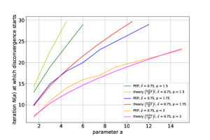
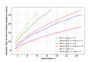
Figure 1: Comparison of theoretical and PEP calculated iteration $N$ after which ISTM with parameter $a$ starts to disconverge for different $p$ under $L=1,R=1$ and Left: $\hat{\varepsilon}=0.75$, Right: $\hat{\varepsilon}=0.75$.

As one can see theoretical and numerical results in the case of arbitrary $p\in[1,2]$ matches well, especially in terms of the forms of the curves. Constant $C$ at which the smallest error of approximation is achieved is $C\sim 4.5$.

Experiment 2.

In this experiment, we study the effect of intermediate acceleration on plateau values that ISTM achieves. By convergence formula (10) from Theorem 3.1,

$$f(y^{N})-f(x^{*})\leq O\left(\max\left\{\frac{LR_{0}^{2}}{N^{p}},\frac{\sqrt{\hat{\varepsilon}}LR_{0}^{2}}{N^{\frac{3p}{4}}},\frac{\hat{\varepsilon}LR_{0}^{2}}{N^{\frac{p}{2}}},\hat{\varepsilon}^{2}LR_{0}^{2},\right\}\right)$$

the plateau level at which the algorithm begins to oscillate after a large number of iterations $N$ does not depend on $p$ and equals $LR_{0}^{2}\hat{\varepsilon}^{2}$. To do this, we consider solving maximization problem (8.2) $\tau^{N}=\max_{f}f(y^{N})-f(x^{*})$ setting the parameter $a$ of ISTM to $\max\left\{1,N^{\frac{p}{4}}\sqrt{\hat{\varepsilon}},N^{\frac{p}{2}}\hat{\varepsilon},N^{p}\hat{\varepsilon}^{2}\right\}$.

Fig. 2 shows the convergence of ISTM with proper parameter $a$ for different intermediate parameter $p$.

Figure 2: Plateau level that achieve ISTM with different intermediate parameter $p$ and $L=1,R=1,\hat{\varepsilon}=0.95$.

One can observe that there are differences in the rate of convergence to a plateau, but the plateau levels themselves differ very little from each other. Therefore, PEP confirms the results of Theorem 3.1.

PEP Experiments discussion

Based on all the experiments performed, we can conclude that our Theorem 3.1 gives tight estimates for the convergence of ISTM. We conjecture that up to the numerical constant, it is impossible to improve them in terms of robustness to relative noise and convergence rate.

5.2 Comparison of Algorithms 1, 3 and 4.

In this subsection, to demonstrate the performance of the proposed Algorithms 1 (ISTM), 3 (AIM) and 4 (AIM with variable $p$), we conduct some numerical experiments for the considered problem (6), with the following objective function, methods (see Nesterov (2018)).

$$f(x)=\frac{L}{8}\left(x_{1}^{2}+\sum_{i=1}^{n-1}(x_{i}-x_{i+1})^{2}+x_{n}^{2}\right)-\frac{L}{4}x_{1},$$ (45)

for some $L>0$. This function is known as the worst-case function for first-order. It is an $L$-smooth, and for it, we have

$$x^{*}=\left(1-\frac{1}{n+1},1-\frac{2}{n+1},\ldots,1-\frac{n}{n+1}\right)\in\mathbb{R}^{n}.$$

We run Algorithms 1, 3 and 4 with $n=100,L=1,p=2$ with different values of $\hat{\varepsilon}\in[0,1]$. In Algorithm 1 we take $a=2$ and in Algorithms 3 and 4 we take $\delta_{k}=\frac{\hat{\varepsilon}^{2}\|\widetilde{\nabla}f(x^{k})\|_{2}^{2}}{\hat{c}}$, with $\hat{c}=1000$.

The results of the work of these compared algorithms are represented in Fig. 3, below. These results demonstrate the difference $f(y^{k})-f(x^{*})$ at each iteration and theoretical estimates (14) (for ISTM), and estimates (35) (which is labeled in the figure by ”AIM (estimate 1)”), (36) (which is labeled in the figure by ”AIM (estimate 2)”) for AIM.

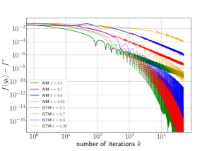
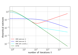
Figure 3: The results of ISTM (Algorithm 1), AIM (Algorithm 3) and AIM with variable $p$ (Algorithm 4) for the objective function (45) with different values of $\hat{\varepsilon}\in[0,1]$.

From Fig. 3, for the objective function (45), we see that through ISTM, we can, for not big values of the parameter $a$, obtain better minimal values for the objective function than the values we obtain through AIM (when we increase the value of $a$, at the first iterations of AIM will give better minimal values of the objective than ISTM, see also Fig. 9). Also, for the received theoretical estimates, we can see that ISTM gives a better estimate of a solution when $p=2$ and for not big values of $a$. When we decrease the value of $p$ and increase $a$, AIM will give better estimates. Also, note that the estimate (35) is without any distortion, and it is adaptive where we always can implement it for any smooth objective function without any additional information about the parameters such that $L$.

Also, from Fig. 3, we can see the efficiency of the proposed Algorithm 4 (AIM with variable $p$), whereby this algorithm we can obtain a solution of the problem with a better estimate.

More additional experiments, for Algorithms 1, 3 and 4, can be found in Subsection 8.5.

6 Conclusions and future plans

In this work for convex functions, we showed that ISTM convergences to $\hat{\varepsilon}^{2}LR_{0}^{2}$ plateau with rate $\sim\frac{1}{N^{p}}$ for any intermediate parameter $p\in[1,2].$ Moreover, for strongly convex functions we found a new lower bound $\hat{\varepsilon}\lesssim\left(\frac{\mu}{L}\right)^{\frac{1}{2}}$ under which relative noise $\hat{\varepsilon}$ does not affect convergence rate. We obtained it using ISTM for convex and smooth functions and restart technique. However, there exists a variant of ISTM Algorithm especially for strongly convex functions from work Gorbunov et al. (2019). In the future, we plan to study it with relative noise and, probably, get new bounds on $\hat{\varepsilon}$ and better understatement of the role of intermediate parameter $p$.

With the help of PEP, we showed that our theoretical results for ISTM are about to be tight. In the future following the work Taylor and Drori (2023) we plan to find the optimal Intermediate Method and coefficients for it under fixed $\varepsilon,p.$

We also proposed adaptive algorithms (AIM, AIM with variable $p$) for the constrained optimization problem. We investigated adaptivity w.r.t. both Lipschitz smoothness and intermediate parameter $p$. The adaptivity w.r.t. parameter $p$ along the iteration process, leads to better robustness and a better estimate of a solution to the problem under consideration. We left the study of the adaptive approaches for problems with strongly convex function and relative noise in the gradient as future work.

7 Acknowledgments

This work was supported by a grant for research centers in the field of artificial intelligence, provided by the Analytical Center for the Government of the Russian Federation in accordance with the subsidy agreement (agreement identifier 000000D730321P5Q0002) and the agreement with the Moscow Institute of Physics and Technology dated November 1, 2021 No. 70-2021-00138.

8 Appendix

8.1 ISTM missing proofs

In this section, we provide full proofs of technical lemmas and the main theorems. First of all, the following technical lemma allows us to obtain estimates for the size of parameter $A_{k}$.

Lemma 8.1.

Consider two sequences of non-negative numbers $\{\alpha_{k}\}_{k\geq 0}$ and $\{A_{k}\}_{k\geq 0}$ such that

$$\alpha_{0}=A_{0}=0,\quad A_{k+1}=A_{k}+\alpha_{k+1},\quad\alpha_{k+1}=\frac{(k+2)^{p-1}}{2aL}\quad\forall k\geq 0,$$ (46)

where $a\geq 1,L>0$. Then for all $k\geq 0$

$$A_{k+1} \geq aL\alpha_{k+1}^{2},$$ (47)

$$A_{k+1} \geq \frac{(k+2)^{p}}{4aL}.$$ (48)

For $p=2$, the explicit formula of $A_{k+1}$ looks like

$$A_{k+1}=\frac{(k+1)(k+4)}{4aL}.$$ (49)

Proof.

With $\alpha_{0}=A_{0}=0$, we write down $A_{k+1}$ as

$$A_{k+1} = \sum_{m=1}^{k+1}\alpha_{m}=\frac{1}{2aL}\sum_{m=1}^{k+1}(m+1)^{p-1}$$

$$\geq \frac{1}{2aL}\int_{0}^{k+1}(x+1)^{p-1}dx=\frac{(k+2)^{p}}{2aLp}-\frac{1}{2aLp}.$$

Because of $1\leq p\leq 2$, we have

$$A_{k+1}\geq\frac{(k+2)^{p}}{4aL}+\frac{1}{2aL}\geq\frac{(k+2)^{p}}{4aL},\quad\forall k\geq 1.$$

We notice that $\forall p\in[1,2]:p\geq 2p-2$. Thus, due to (48), we get

$$A_{k+1}\geq\frac{(k+2)^{p}}{4aL}\geq aL\frac{(k+2)^{2p-2}}{4a^{2}L^{2}}=aL\alpha_{k+1}^{2},\quad\forall k\geq 0.$$

Finally, for $p=2$, the explicit formula looks like $A_{k+1}=\frac{1}{2aL}\sum_{m=1}^{k+1}(m+1)$. Using fact that $\sum_{m=1}^{k+1}(m+1)=\frac{(k+1)(k+4)}{2}$ we complete the proof. ∎

The next lemma provides details of the general convergence of Algorithm 1 with arbitrary coefficients $\{A_{k}\},\{\alpha_{k}\}$.

Lemma 8.2.

Gorbunov et al. [2020] Let $f$ be convex function (Assumption 1) and $L$-smooth (Assumption 2). Let the stepsize parameter $a$ satisfies $a\geq 1$ and for coefficients $\{A_{k}\},\{\alpha_{k}\}$ inequality (47) holds true. Then after $N\geq 0$ iterations of Algorithm 1 with coefficients $\{A_{k}\},\{\alpha_{k}\}$ for all $z\in\mathbb{R}^{n}$ we have

$$A_{N}(f(y^{N})-f(z))\leq \frac{1}{2}\left\|z^{0}-z\right\|_{2}^{2}-\frac{1}{2}\left\|z^{N}-z\right\|_{2}^{2}+\sum_{k=0}^{N-1}\alpha_{k+1}\left\langle\theta_{k+1},z-z^{k}\right\rangle$$

$$+\sum_{k=0}^{N-1}\alpha_{k+1}^{2}\left\|\theta_{k+1}\right\|_{2}^{2}+\sum_{k=0}^{N-1}\alpha_{k+1}^{2}\left\langle\theta_{k+1},\nabla f(x^{k+1})\right\rangle,$$

where

$$\theta_{k+1}:=\widetilde{\nabla}f(x^{k+1})-\nabla f(x^{k+1}).$$

Full proof of Theorem 3.1

Firstly, we complete the proof in a particular case, when $p=2$ (which is the classical Similar Triangle Method (STM)), and then generalize it for all $p\in[1,2].$

Classic STM.

From Lemma 8.2, for any $N\geq 0$, we have

$$A_{N}(f(y^{N})-f(x^{*}))\leq \frac{1}{2}\left\|z^{0}-x^{*}\right\|_{2}^{2}-\frac{1}{2}\left\|z^{N}-x^{*}\right\|_{2}^{2}$$ (50)

$$+\sum_{k=0}^{N-1}\alpha_{k+1}\left\langle\theta_{k+1},x^{*}-z^{k}\right\rangle+\sum_{k=0}^{N-1}\alpha_{k+1}^{2}\left\|\theta_{k+1}\right\|_{2}^{2}$$

$$+\sum_{k=0}^{N-1}\alpha_{k+1}^{2}\left\langle\theta_{k+1},\nabla f(x^{k+1})\right\rangle.$$

Taking into account that $f(y^{N})-f(x^{*})\geq 0$, for all $y^{N}$, and using the notation $R_{k}:=\|z^{k}-x^{*}\|_{2}$, we find that for all $0\leq k\leq N$

$$R_{k}^{2} \leq R_{0}^{2}+2\sum_{l=0}^{k-1}\alpha_{l+1}\left\langle\theta_{l+1},x^{*}-z^{l}\right\rangle+2\sum_{l=0}^{k-1}\alpha_{l+1}^{2}\left\langle\theta_{l+1},\nabla f\left(x^{l+1}\right)\right\rangle$$ (51)

$$\;\;\;\;+2\sum_{l=0}^{k-1}\alpha_{l+1}^{2}\left\|\theta_{l+1}\right\|_{2}^{2}.$$

Now, let us prove by the induction, that the inequalities

$$R_{k}^{2} \stackrel{{\scriptstyle\eqref{eq_64}}}{{\leq}}R_{0}^{2}+2\sum_{l=0}^{k-1}\alpha_{l+1}\left\langle\theta_{l+1},x^{*}-z^{l}\right\rangle+2\sum_{l=0}^{k-1}\alpha_{l+1}^{2}\left\langle\theta_{l+1},\nabla f\left(x^{l+1}\right)\right\rangle$$ (52)

$$\;\;\;\;+2\sum_{l=0}^{k-1}\alpha_{l+1}^{2}\left\|\theta_{l+1}\right\|_{2}^{2}\leq C_{1}^{2}R_{0}^{2},$$

hold for $k=0,\ldots,N$ simultaneously, where $C_{1}$ is defined in (9).

For $t=0$, the inequality (52) holds since $C_{1}\geq 1$. Now, let us assume (induction hypothesis) that (52) holds for some $k=T-1\leq N-1$ and prove it for $k=T\leq N$.

From (50), we find that

$$f(y^{t})-f(x^{*}) \leq\frac{1}{2A_{t}}\Big{(}R_{0}^{2}+2\sum_{l=0}^{t-1}\alpha_{l+1}\left\langle\theta_{l+1},x^{*}-z^{l}\right\rangle+$$

$$\;\;\;\;+2\sum_{l=0}^{t-1}\alpha_{l+1}^{2}\left\langle\theta_{l+1},\nabla f\left(x^{l+1}\right)\right\rangle+2\sum_{l=0}^{t-1}\alpha_{k+1}^{2}\left\|\theta_{l+1}\right\|_{2}^{2}\Big{)},$$

holds for $t=1,\ldots,T-1$. Therefore, because of (52), the next inequality also holds true

$$f(y^{t})-f(x^{*})\leq\frac{C_{1}^{2}R_{0}^{2}}{2A_{t}},\quad t=1,\ldots,T-1.$$ (53)

By line $4$ of Algorithm 1 we have $x^{1}=\frac{1}{A_{1}}(A_{0}y^{0}+\alpha_{1}z^{0})$. However, $A_{0}=0$ and from line $3$ of of Algorithm 1,we get

$$A_{1}=\alpha_{1},\quad\text{and}\quad\alpha_{1}=\frac{1}{aL}\Longrightarrow L=\frac{1}{a\alpha_{1}}.$$

Consequently, $x^{1}=z^{0}$, and we bound $\left\|\nabla f\left(x^{1}\right)\right\|_{2}$ at the first iteration as follows

$$\left\|\nabla f(x^{1})\right\|_{2} =\left\|\left(\nabla f(z^{0})-\widetilde{\nabla}f(z^{0})\right)+\left(\widetilde{\nabla}f(z^{0})-\nabla f(z^{0})\right)+\nabla f(z^{0})\right\|_{2}$$

$$\leq 2\left\|\widetilde{\nabla}f(z^{0})-\nabla f(z^{0})\right\|_{2}+\left\|\nabla f(z^{0})\right\|_{2}$$

$$\leq(2\hat{\varepsilon}+1)\left\|\nabla f(z^{0})\right\|_{2}$$

$$\leq(2\hat{\varepsilon}+1)\left\|\nabla f(z^{0})-\nabla f(x^{*})\right\|_{2}$$

$$\stackrel{{\scriptstyle\eqref{eq_6}}}{{\leq}}(2\hat{\varepsilon}+1)L\left\|z^{0}-x^{*}\right\|_{2}=\frac{(2\hat{\varepsilon}+1)R_{0}}{a\alpha_{1}}.$$

Also, for $t=0,1,\ldots,T-1$, we have

$$\left\|\nabla f(x^{t+1})\right\|_{2} \;\;\leq\left\|\nabla f(x^{t+1})-\nabla f(y^{t})\right\|_{2}+\left\|\nabla f(y^{t})\right\|_{2}$$

$$\stackrel{{\scriptstyle\eqref{eq_6},\eqref{eq_8}}}{{\leq}}L\left\|x^{t+1}-y^{t}\right\|_{2}+\sqrt{2L\left(f(y^{t})-f(x^{*})\right)}.$$

From the definition of $x^{k+1}$ (see line $4$ of Algorithm 1) and since $A_{k+1}=\alpha_{k+1}+A_{k}$ (see line $3$ of Algorithm 1), we have

$$(\alpha_{k+1}+A_{k})x^{k+1}=A_{k}y^{k}+\alpha_{k+1}z^{k},$$

i.e.

$$x^{k+1}-y^{k}=\frac{\alpha_{k+1}}{A_{k}}(z^{k}-x^{k+1}).$$ (54)

Let $\widetilde{R}_{0}:=R_{0},\widetilde{R}_{k+1}:=\max\{\widetilde{R}_{k},R_{k+1}\}$. From (53) and (54), and since $\alpha_{k+1}=\frac{k+2}{2aL}$, we get for $t=1,\ldots,T-1$, the following

$$\left\|\nabla f(x^{t+1})\right\|_{2} \leq\frac{\alpha_{t+1}L}{A_{t}}\left\|x^{t+1}-z^{t}\right\|_{2}+\sqrt{\frac{LC_{1}^{2}R_{0}^{2}}{A_{t}}}$$

$$\stackrel{{\scriptstyle\eqref{eq_20}}}{{\leq}}\frac{2L(t+2)}{t(t+3)}\left(\left\|x^{t+1}-x^{*}\right\|_{2}+\left\|x^{*}-z^{t}\right\|_{2}\right)+\frac{2LC_{1}R_{0}\sqrt{a}}{\sqrt{t(t+3)}}$$

$$\leq\frac{4L(t+2)\widetilde{R}_{t}}{t(t+3)}+\frac{2LC_{1}R_{0}\sqrt{a}}{\sqrt{t(t+3)}}$$

$$\stackrel{{\scriptstyle\eqref{eq_65}}}{{\leq}}\frac{4L(t+2)C_{1}R_{0}}{t(t+3)}+\frac{2LC_{1}R_{0}\sqrt{a}}{\sqrt{t(t+3)}}$$

$$\;=4LC_{1}R_{0}\left(\frac{t+2}{t(t+3)}+\frac{\sqrt{a}}{2\sqrt{t(t+3)}}\right)$$

$$=\frac{2C_{1}R_{0}}{\alpha_{t+1}}\left(\frac{(t+2)^{2}}{at(t+3)}+\frac{t+2}{2\sqrt{at(t+3)}}\right).$$

Because of $\frac{(t+2)^{2}}{t(t+3)}\leq\frac{(1+2)^{2}}{1(1+3)}=\frac{9}{4}$, we get, for $t=1,\ldots,T-1$

$$\left\|\nabla f(x^{t+1})\right\|_{2}\leq\frac{C_{1}R_{0}}{\alpha_{t+1}}\left(\frac{9}{2a}+\frac{3}{2\sqrt{a}}\right).$$

Let $\frac{9}{2a}+\frac{3}{2\sqrt{a}}:=\frac{1}{C}$, then we have

$$\left\|\nabla f(x^{t+1})\right\|_{2}\leq\frac{C_{1}R_{0}}{C\alpha_{t+1}},\quad\forall t=1,\ldots,T-1.$$

Now we go back to inequality

$$R_{T}^{2} \leq R_{0}^{2}+\underbrace{2\sum_{l=0}^{T-1}\alpha_{l+1}\left\langle\theta_{l+1},x^{*}-z^{l}\right\rangle}_{\Circled{1}}+\underbrace{2\sum_{l=0}^{T-1}\alpha_{l+1}^{2}\left\|\theta_{l+1}\right\|_{2}^{2}}_{\Circled{2}}$$

$$\;\;\;\;+\underbrace{2\sum_{l=0}^{T-1}\alpha_{l+1}^{2}\left\langle\theta_{l+1},\nabla f(x^{l+1})\right\rangle}_{\Circled{3}},$$

and provide tight upper bounds for $\Circled{1},\Circled{2}$ and $\Circled{3}$.

Upper bound for $\Circled{1}$. We have

$$\left|\Circled{1}\right| \leq 2\sum_{l=0}^{T-1}\alpha_{l+1}\left\langle\theta_{l+1},x^{*}-z^{l}\right\rangle\leq 2\sum_{l=0}^{T-1}\alpha_{l+1}\left\|\theta_{l+1}\right\|_{2}\left\|x^{*}-z^{l}\right\|_{2}$$

$$\leq 2\sum_{l=0}^{T-1}\alpha_{l+1}\hat{\varepsilon}\left\|\nabla f(x^{l+1})\right\|_{2}C_{1}R_{0}\leq 2\sum_{l=0}^{T-1}\alpha_{l+1}\hat{\varepsilon}\frac{C_{1}^{2}R_{0}^{2}}{C\alpha_{l+1}}\stackrel{{\scriptstyle T\leq N}}{{\leq}}\frac{2N\hat{\varepsilon}C_{1}^{2}R_{0}^{2}}{C}.$$

Let us choose $a$ such that

$$\frac{2N\hat{\varepsilon}C_{1}^{2}}{C}\leq\frac{1}{4}\;\Longrightarrow\;\left(\frac{9}{2a}+\frac{3}{2\sqrt{a}}\right)2N\hat{\varepsilon}C_{1}^{2}\leq\frac{1}{4}\;\Longrightarrow\;a\gtrapprox\max\left\{N\hat{\varepsilon},N^{2}\hat{\varepsilon}^{2}\right\},$$ (55)

then we get the following upper bound for $\Circled{1}$

$$2\sum_{l=0}^{T-1}\alpha_{l+1}\left\langle\theta_{l+1},x^{*}-z^{l}\right\rangle\leq\frac{1}{4}R_{0}^{2}.$$

Upper bound for $\Circled{2}$. We have

$$\left|\Circled{2}\right| \leq 2\sum_{l=0}^{T-1}\alpha_{l+1}^{2}\left\|\theta_{l+1}\right\|_{2}^{2}\leq 2\sum_{l=0}^{T-1}\alpha_{l+1}^{2}\hat{\varepsilon}^{2}\left\|\nabla f(x^{l+1})\right\|_{2}^{2}$$

$$\leq 2\sum_{l=0}^{T-1}\alpha_{l+1}^{2}\hat{\varepsilon}^{2}\cdot\frac{C_{1}^{2}R_{0}^{2}}{C^{2}\alpha_{l+1}^{2}}\stackrel{{\scriptstyle T\leq N}}{{\leq}}\;\;\frac{2N\hat{\varepsilon}^{2}C_{1}^{2}R_{0}^{2}}{C^{2}}.$$

Let us choose $a$ such that

$$\frac{2N\hat{\varepsilon}^{2}C_{1}^{2}}{C^{2}}\leq\frac{1}{4}\;\Longrightarrow\;\left(\frac{9}{2a}+\frac{3}{2\sqrt{a}}\right)^{2}2N\hat{\varepsilon}^{2}C_{1}^{2}\leq\frac{1}{4}\;\Longrightarrow\;a\gtrapprox\max\left\{N\hat{\varepsilon}^{2},\sqrt{N}\hat{\varepsilon}\right\},$$ (56)

then we get the following upper bound for $\Circled{2}$

$$2\sum_{l=0}^{T-1}\alpha_{l+1}^{2}\left\|\theta_{l+1}\right\|_{2}^{2}\leq\frac{1}{4}R_{0}^{2}.$$

Upper bound for $\Circled{3}$. We have

$$\left|\Circled{3}\right| \leq 2\sum_{l=0}^{T-1}\alpha_{l+1}^{2}\left\langle\theta_{l+1},\nabla f(x^{l+1})\right\rangle\leq 2\sum_{l=0}^{T-1}\alpha_{l+1}^{2}\left\|\theta_{l+1}\right\|_{2}\left\|\nabla f(x^{l+1})\right\|_{2}$$

$$\leq 2\sum_{l=0}^{T-1}\alpha_{l+1}^{2}\hat{\varepsilon}\left\|\nabla f(x^{l+1})\right\|_{2}^{2}\leq 2\sum_{l=0}^{T-1}\alpha_{l+1}^{2}\hat{\varepsilon}\,\frac{C_{1}^{2}R_{0}^{2}}{C^{2}\alpha_{l+1}^{2}}\stackrel{{\scriptstyle T\leq N}}{{\leq}}\;\;\frac{2N\hat{\varepsilon}C_{1}^{2}R_{0}^{2}}{C^{2}}.$$

Let us choose $a$ such that

$$\frac{2N\hat{\varepsilon}C_{1}^{2}}{C^{2}}\leq\frac{1}{4}\;\Longrightarrow\;\left(\frac{9}{2a}+\frac{3}{2\sqrt{a}}\right)^{2}2N\hat{\varepsilon}C_{1}^{2}\leq\frac{1}{4}\;\Longrightarrow\;a\gtrapprox\max\left\{\sqrt{N\hat{\varepsilon}},N\hat{\varepsilon}\right\},$$ (57)

then we get the following upper bound for $\Circled{3}$

$$2\sum_{l=0}^{T-1}\alpha_{l+1}^{2}\left\langle\theta_{l+1},\nabla f(x^{l+1})\right\rangle\leq\frac{1}{4}R_{0}^{2}.$$

Consequently, we find that

$$R_{T}^{2} \leq R_{0}^{2}+\frac{3}{4}R_{0}^{2}=\frac{7}{4}R_{0}^{2}\leq C_{1}^{2}R_{0}^{2},\quad\text{where}\,\,C_{1}=\sqrt{2}.$$

As a result, for every $N\geq 0$, we have

$$R_{k}^{2}\leq 2R_{0}^{2},\quad\forall\,k=0,1,\ldots,N.$$ (58)

Now, from (50), (52) and (58), we have

$$A_{N}\left(f(y^{N})-f(x^{*})\right) \leq R_{0}^{2}+2\sum_{k=0}^{N-1}\alpha_{k+1}\left\langle\theta_{k+1},x^{*}-z^{k}\right\rangle+2\sum_{k=0}^{N-1}\alpha_{k+1}^{2}\left\|\theta_{k+1}\right\|_{2}^{2}$$

$$\;\;\;\;+2\sum_{k=0}^{N-1}\alpha_{k+1}^{2}\left\langle\theta_{k+1},\nabla f(x^{k+1})\right\rangle$$

$$\leq 2R_{0}^{2}.$$

Consequently, we get from Lemma 49, the following inequality

$$f(y^{N})-f(x^{*})\leq\frac{2R_{0}^{2}}{A_{N}}=\frac{8aLR_{0}^{2}}{N(N+3)}.$$

From (55), (56) and (57) we find that if we choose $a$, such that

$$a=O\left(\max\left\{1,\sqrt{N\hat{\varepsilon}},N\hat{\varepsilon},N^{2}\hat{\varepsilon}^{2}\right\}\right),$$

with $\hat{\varepsilon}\in[0,1]$, then we get

$$f(y^{N})-f(x^{*})\leq O\left(\max\left\{\frac{LR_{0}^{2}}{N^{2}},\frac{\sqrt{\hat{\varepsilon}}LR_{0}^{2}}{\sqrt{N^{3}}},\frac{\hat{\varepsilon}LR_{0}^{2}}{N},\hat{\varepsilon}^{2}LR_{0}^{2}\right\}\right).$$

Power policy (generalization to $p\in[1,2]$).

For the case when $p\in[1,2]$, the Lemma 8.2 is still valid with $\alpha_{k+1},A_{k+1}$ in (46), but the bound for $\left\|\nabla f(x^{t+1})\right\|_{2}$ in each step is different, which can be shown as follows.

Firstly, for $\forall t=1,2,\ldots,T-1$, we have

$$\left\|\nabla f(x^{t+1})\right\|_{2} \leq\frac{\alpha_{t+1}}{A_{t}}2L\widetilde{R}_{t}+\frac{\sqrt{L}C_{1}R_{0}}{\sqrt{A_{t}}}$$

$$\leq 4LC_{1}R_{0}\frac{(t+2)^{p-1}}{(t+1)^{p}}+\frac{2\sqrt{a}LC_{1}R_{0}}{(t+1)^{p/2}}$$

$$\leq\frac{4aLC_{1}R_{0}}{(t+1)^{p/2}}\left(\frac{(t+2)^{p-1}}{a(t+1)^{p/2}}+\frac{1}{2\sqrt{a}(t+1)^{p}}\right).$$

Because of $p\in[1,2]$, we find $p-1\leq\frac{p}{2}\leq 1$, and

$$\frac{(t+2)^{p}}{(t+1)^{p/2}}\leq\frac{3^{p-1}}{2^{p/2}}\leq\frac{3}{\sqrt{2}},\quad\text{and}\quad\frac{1}{(t+1)^{p}}\leq\frac{1}{2^{p}}\leq\frac{1}{2}.$$

Consequently, we get, for $t=1,\ldots,T-1$, the following

$$\left\|\nabla f(x^{t+1})\right\|_{2}\leq\frac{4aLC_{1}R_{0}}{(t+1)^{p/2}}\left(\frac{3}{\sqrt{2}a}+\frac{1}{4\sqrt{a}}\right)=\frac{4aLC_{1}R_{0}}{\widetilde{C}(t+1)^{p/2}},$$ (59)

where $\frac{1}{\widetilde{C}}:=\frac{3}{\sqrt{2}a}+\frac{1}{4\sqrt{a}}$.

Now, with (46), (59), in a similar way as previously, for the upper bound for $\Circled{1}$, we have

$$\left|\Circled{1}\right| \leq 2\sum_{l=0}^{T-1}\alpha_{l+1}\left\langle\theta_{l+1},x^{*}-z^{l}\right\rangle\leq\frac{4C_{1}^{2}R_{0}^{2}\hat{\varepsilon}}{\widetilde{C}}\sum_{l=0}^{T-1}\frac{(l+2)^{p-1}}{(l+1)^{p/2}}$$

$$\leq\frac{4C_{1}^{2}R_{0}^{2}\hat{\varepsilon}}{\widetilde{C}}\sum_{l=0}^{T}l^{\frac{p}{2}-1}\leq\frac{4C_{1}^{2}R_{0}^{2}\hat{\varepsilon}}{\widetilde{C}}TT^{\frac{p}{2}-1}\;\stackrel{{\scriptstyle T\leq N}}{{\leq}}\;\;\frac{4C_{1}^{2}R_{0}^{2}\hat{\varepsilon}N^{p/2}}{\widetilde{C}}.$$

Let us choose $a$ such that

$$\frac{4C_{1}^{2}\hat{\varepsilon}N^{p/2}}{\widetilde{C}}\leq\frac{1}{4} \Longrightarrow\;\left(\frac{3}{\sqrt{2}a}+\frac{1}{4\sqrt{a}}\right)4C_{1}^{2}\hat{\varepsilon}N^{p/2}\leq\frac{1}{4}$$ (60)

$$\Longrightarrow\;a\gtrapprox\max\left\{\hat{\varepsilon}N^{p/2},\hat{\varepsilon}^{2}N^{p}\right\},$$

then we get $\left|\Circled{1}\right|\leq\frac{R_{0}^{2}}{4}$.

For the upper bound for $\Circled{2}$ (with (46), (59)), we have

$$\left|\Circled{2}\right| \leq 2\sum_{l=0}^{T-1}\alpha_{l+1}^{2}\left\|\theta_{l+1}\right\|_{2}^{2}\leq 2\sum_{l=0}^{T-1}\alpha_{l+1}^{2}\hat{\varepsilon}^{2}\left\|\nabla f(x^{l+1})\right\|_{2}^{2}$$

$$\leq 2\sum_{l=0}^{T-1}\frac{(l+2)^{2p-2}}{4a^{2}L^{2}}\cdot\hat{\varepsilon}^{2}\frac{16a^{2}L^{2}C_{1}^{2}R_{0}^{2}}{\widetilde{C}^{2}(l+1)^{p}}\leq\frac{8\hat{\varepsilon}^{2}C_{1}^{2}R_{0}^{2}}{\widetilde{C}^{2}}\sum_{l=0}^{T}\frac{(l+2)^{2p-2}}{(l+1)^{p}}$$

$$\leq\frac{8\hat{\varepsilon}^{2}C_{1}^{2}R_{0}^{2}}{\widetilde{C}^{2}}\sum_{l=0}^{T}l^{\frac{p}{2}-1}\;\stackrel{{\scriptstyle T\leq N}}{{\leq}}\;\;\frac{8\hat{\varepsilon}^{2}C_{1}^{2}R_{0}^{2}N^{p/2}}{\widetilde{C}^{2}}.$$

Let us choose $a$ such that

$$\frac{8\hat{\varepsilon}^{2}C_{1}^{2}N^{p/2}}{\widetilde{C}^{2}}\leq\frac{1}{4} \Longrightarrow\;\left(\frac{3}{\sqrt{2}a}+\frac{1}{4\sqrt{a}}\right)^{2}8C_{1}^{2}\hat{\varepsilon}^{2}N^{p/2}\leq\frac{1}{4}$$ (61)

$$\Longrightarrow\;a\gtrapprox\max\left\{\hat{\varepsilon}N^{p/4},\hat{\varepsilon}^{2}N^{p/2}\right\},$$

then we get $\left|\Circled{2}\right|\leq\frac{R_{0}^{2}}{4}$.

For the upper bound for $\Circled{3}$ (with (46), (59)), we have

$$\left|\Circled{3}\right| \leq 2\sum_{l=0}^{T-1}\alpha_{l+1}^{2}\left\langle\theta_{l+1},\nabla f(x^{l+1})\right\rangle\leq 2\sum_{l=0}^{T-1}\alpha_{l+1}^{2}\hat{\varepsilon}\left\|\nabla f(x^{l+1})\right\|_{2}^{2}$$

$$\leq\frac{8\hat{\varepsilon}C_{1}^{2}R_{0}^{2}}{\widetilde{C}^{2}}\sum_{l=0}^{T}\frac{(l+2)^{2p-2}}{(l+1)^{p}}\;\stackrel{{\scriptstyle T\leq N}}{{\leq}}\;\;\frac{8\hat{\varepsilon}C_{1}^{2}R_{0}^{2}N^{p/2}}{\widetilde{C}^{2}}.$$

Let us choose $a$ such that

$$\frac{8\hat{\varepsilon}C_{1}^{2}N^{p/2}}{\widetilde{C}^{2}}\leq\frac{1}{4} \Longrightarrow\;\left(\frac{3}{\sqrt{2}a}+\frac{1}{4\sqrt{a}}\right)^{2}8C_{1}^{2}\hat{\varepsilon}N^{p/2}\leq\frac{1}{4}$$ (62)

$$\Longrightarrow\;a\gtrapprox\max\left\{\sqrt{\hat{\varepsilon}}N^{p/4},\hat{\varepsilon}N^{p/2}\right\},$$

then we get $\left|\Circled{3}\right|\leq\frac{R_{0}^{2}}{4}$.

Therefore, for ISTM, we have

$$f(y^{N})-f(x^{*})\leq\frac{2R_{0}^{2}}{A_{N}}\leq\frac{8aLR_{0}^{2}}{(N+1)^{p}},$$ (63)

and from (60), (61) and (62), we find that by choosing $a$, such that

$$a=O\left(\max\left\{1,\sqrt{\hat{\varepsilon}}N^{p/4},\hat{\varepsilon}N^{p/2},\hat{\varepsilon}^{2}N^{p}\right\}\right),$$ (64)

with $\hat{\varepsilon}\in[0,1]$, and $p\in[1,2]$, we get

$$f(y^{N})-f(x^{*})\leq O\left(\max\left\{\frac{LR_{0}^{2}}{N^{p}},\frac{\sqrt{\hat{\varepsilon}}LR_{0}^{2}}{N^{3p/4}},\frac{\hat{\varepsilon}LR_{0}^{2}}{N^{p/2}},\hat{\varepsilon}^{2}LR_{0}^{2}\right\}\right).$$ (65)

8.2 Additional details about PEP

In order to find tight convergence rate for ISTM Algorithm 1, we consider the following optimization problem with fixed $N,\hat{\varepsilon},a$

$$\max\limits_{n,f,x^{0}} f(x^{N})-f(x^{*})$$

$$f:\mathbb{R}^{n}\rightarrow\mathbb{R}\text{ is $L$ -smooth and convex},$$

$$0\in\nabla f(x^{*}),$$

$$\|x^{0}-x^{*}\|^{2}_{2}\leq R^{2},$$

$$\|\widetilde{\nabla}f(x^{k})-\nabla f(x^{k})\|^{2}_{2}\leq\hat{\varepsilon}^{2}\|\nabla f(x^{k})\|^{2}_{2},\quad k=\overline{0,N-1},$$

$$x^{k+1},y^{k+1},z^{k+1}=\text{ISTMstep}(x^{k},y^{k},z^{k},\widetilde{\nabla}f(x^{k})),\quad k=\overline{0,N-1}.$$

In this problem, we produce maximization over an infinitely dimensional domain of $L$ -smooth and convex functions. For numerical experiments problem (8.2) can be equivalently reformulated in finite-dimensional convex optimization task. This reformulation baseline was introduced in Drori and Teboulle [2014] and further developed for convex and $L$-smooth optimization in Taylor et al. [2017]. For the problems with relative inaccuracy in the gradients, this problem is also studied in De Klerk et al. [2017]. We will consider maximization over the set of triplets that represent points and function’s values and gradients. We denote this index set $I=\{*,0,1,\dots,N\}$. The equivalent problem takes the following form

$$\max\limits_{\begin{subarray}{k}n,x^{*},f^{*},g^{*}\\ \{x^{i},y^{i},z^{i}\}_{i=0}^{N}\\ \{f^{i},g^{i},\widetilde{g}^{i}\}_{i=0}^{N}\end{subarray}} f^{N}-f^{*}$$

$$f:\mathbb{R}^{n}\rightarrow\mathbb{R}\text{ is $L$ -smooth and convex},$$

$$f^{k}=f(x^{k}),\quad g^{k}\in\nabla f(x^{k}),\quad k=*,0,1\dots,N,$$

$$g^{*}=0,$$

$$\|x^{0}-x^{*}\|^{2}_{2}\leq R^{2},$$

$$\|\widetilde{g}^{k}-g^{k}\|^{2}_{2}\leq\hat{\varepsilon}^{2}\|g^{k}\|^{2}_{2},\quad k=\overline{0,N-1},$$

$$x^{k+1},y^{k+1},z^{k+1}=\text{ISTMstep}(x^{k},y^{k},z^{k},\widetilde{g}^{k}),\hskip 4.26773ptk=\overline{0,N-1}.$$

Harsh conditions (8.2)-(8.2) can be replaced by finite set of conditions on points $\{x^{i}\}_{i\in I}$, function values $\{f^{i}\}_{i\in I}$ and gradients $\{g^{i}\}_{i\in I}$. They allow interpolating the unique $L$-smooth and convex function $f$.

Theorem 8.1.

Taylor et al. [2017] For the set $\{x^{i},f^{i},g^{i}\}_{i\in I}$ there exists convex (Assumption 1) and $L$-smooth (Assumption 2) function $f$ such that for all $i\in I$ we have $g^{i}\in\partial f(x^{i})$ and $f^{i}=f(x^{i})$ if and only if the following condition holds for every pair of indices $i\in I$ and $j\in I$

$$f^{i}-f^{j}-(g^{j})^{\top}(x_{i}-x_{j})\geq\frac{\|g^{i}-g^{j}\|^{2}}{2}.$$ (69)

Using Theorem 8.1, we reduce conditions (8.2)-(8.2) to $(N+2)\times(N+1)$ quadratic (69) type inequalities. Thus, the following problem is equivalent reformulation of problem (8.2)

$$\max\limits_{\begin{subarray}{k}n,x^{*},f^{*},g^{*}\\ \{x^{i},y^{i},z^{i}\}_{i=0}^{N}\\ \{f^{i},g^{i},\widetilde{g}^{i}\}_{i=0}^{N}\end{subarray}} f^{N}-f^{*}$$

$$f^{i}-f^{j}-(g^{j})^{\top}(x_{i}-x_{j})\geq\frac{\|g^{i}-g^{j}\|_{2}^{2}}{2},\hskip 4.26773pti,j=*,0,\dots,N,$$

$$g^{*}=0,$$

$$\|x^{0}-x^{*}\|^{2}_{2}\leq R^{2},$$

$$\|\widetilde{g}^{k}-g^{k}\|^{2}_{2}\leq\hat{\varepsilon}^{2}\|g^{k}\|^{2}_{2},\quad k=\overline{0,N-1},$$

$$x^{k+1},y^{k+1},z^{k+1}=\text{ISTMstep}(x^{k},y^{k},z^{k},\widetilde{g}^{k}),\hskip 4.26773ptk=\overline{0,N-1}.$$

Points $\{x^{i}\}_{i=1}^{N},\{y^{i}\}_{i=0}^{N},\{z^{i}\}_{i=0}^{N}$ are linear combinations of $x_{0},\{\widetilde{g}^{i}\}_{i=0}^{N}$, consequently, we maximize only $2+2*(N+1)$ namely vectors $x^{0},x^{*},\{g^{i}\}_{i\in I},\{\widetilde{g}^{i}\}_{i\in I}$ and $N+1$ scalars $\{f^{i}\}_{i\in I}$. Moreover, the above problem is linear w.r.t. the inner products of all possible pairs of vectors and scalars. Firstly, we define Gram matrix $G:=V^{\top}V\in\mathbb{R}^{2(N+2)\times 2(N+2)}$, where $V=\left(x^{0},x^{*},\{g^{i}\}_{i\in I},\{\widetilde{g}^{i}\}_{i\in I}\right)\in\mathbb{R}^{d\times 2(N+2)}$ and $\mathbf{f}=\left(f_{*},f_{0},\dots,f_{N}\right)\in\mathbb{R}^{N+2}$. With these notations, we can rewrite the problem in SDP form

$$\max\limits_{n,G,\mathbf{f}\in\mathbb{R}^{N+2}} f^{N}-f^{*}$$

$$\mathrm{Tr}(M_{i,j}G)\leq f^{i}-f^{j},\quad i,j=*,0,1\dots,N$$

$$\mathrm{Tr}(M_{*}G)=0,$$

$$\mathrm{Tr}(M_{R}G)\leq R^{2},$$

$$\mathrm{Tr}(N_{i}G)\leq 0,\quad i=0,1,\dots,N-1,$$

$$G\succeq 0,$$

where $M_{i,j}$ represents interpolation conditions (8.2), $M_{*}$ — optimal condition (8.2), $M_{R}$ — initial point condition (8.2) and $N_{i}$ — relative noise conditions (8.2). Due to the cumbersome nature of the matrices, we will not write out their explicit form, however, the algorithm for their construction can be found in the work Taylor et al. [2017]. Note, that in the framework PEPit Goujaud et al. [2022] that we used for numerical experiments, these matrices and the conversion to the SDP form are done automatically.

8.3 AIM missing proofs

Proof of Lemma 4.1

Proof.

We prove this Lemma by induction. For $k=0$, we have

$$\Psi_{0}^{*} \;\;\;\;=\min_{x\in Q}\left\{\Psi_{0}(x)=\frac{1}{2}\|x-x^{0}\|_{2}^{2}+\alpha_{0}f(x^{0})+\alpha_{0}\left\langle\widetilde{\nabla}f(x^{0}),x-x^{0}\right\rangle\right\}$$

$$\;\;\;\stackrel{{\scriptstyle\eqref{y0_adaptive_alg}}}{{\geq}}\alpha_{0}\left(\frac{1}{2\alpha_{0}}\|y^{0}-x^{0}\|_{2}^{2}+f(x^{0})+\left\langle\widetilde{\nabla}f(x^{0}),y^{0}-x^{0}\right\rangle\right)$$

$$\;\;\;\;=\alpha_{0}\left(f(x^{0})+\left\langle\widetilde{\nabla}f(x^{0}),y^{0}-x^{0}\right\rangle+\frac{2^{i_{0}}L_{s}}{2}\|y^{0}-x^{0}\|_{2}^{2}\right)$$

$$\;\;\;\;\geq\alpha_{0}f(y^{0})-\alpha_{0}\delta_{0}=A_{0}f(y^{0})-\alpha_{0}\delta_{0}=A_{0}f(y^{0})-M_{0}.$$

Assume that (33) is valid for certain $k-1\geq 0$, i.e.

$$A_{k-1}f(y^{k-1})-M_{k-1}\leq\Psi_{k-1}^{*},$$ (74)

and let us prove that it holds for $k$. Firstly, we write down $\Psi_{k}^{*}$ based on Algorithm 3 steps, i.e.

$$\Psi_{k}^{*} =\min_{x\in Q}\Psi_{k}(x^{k})\stackrel{{\scriptstyle\eqref{zk_adaptive_alg}}}{{\geq}}\Psi_{k}(z^{k})\stackrel{{\scriptstyle\eqref{psi_star}}}{{=}}\Psi_{k-1}(z^{k})+\alpha_{k}\left(f(x^{k})+\left\langle\widetilde{\nabla}f(x^{k}),z^{k}-x^{k}\right\rangle\right)$$

$$\stackrel{{\scriptstyle\eqref{zk_adaptive_alg}}}{{\geq}}\Psi_{k-1}(z^{k-1})+\frac{1}{2}\left\|z^{k}-z^{k-1}\right\|_{2}^{2}+\alpha_{k}\left(f(x^{k})+\left\langle\widetilde{\nabla}f(x^{k}),z^{k}-x^{k}\right\rangle\right)$$

$$\stackrel{{\scriptstyle\eqref{psi_star}}}{{\geq}}\Psi_{k-1}^{*}+\frac{1}{2}\left\|z^{k}-z^{k-1}\right\|_{2}^{2}+\alpha_{k}\left(f(x^{k})+\left\langle\widetilde{\nabla}f(x^{k}),z^{k}-x^{k}\right\rangle\right)$$

$$\stackrel{{\scriptstyle\eqref{induction_k_1}}}{{\geq}}A_{k-1}f(y^{k-1})-M_{k-1}+\frac{1}{2}\left\|z^{k}-z^{k-1}\right\|_{2}^{2}$$

$$\;\;\;\;+\alpha_{k}\left(f(x^{k})+\left\langle\widetilde{\nabla}f(x^{k}),z^{k}-x^{k}\right\rangle\right)$$

$$\stackrel{{\scriptstyle\eqref{Ak_adaptive_alg}}}{{\geq}}(A_{k}-\alpha_{k})f(y^{k-1})-M_{k-1}+\frac{1}{2}\left\|z^{k}-z^{k-1}\right\|_{2}^{2}$$

$$\;\;\;\;+\alpha_{k}\left(f(x^{k})+\left\langle\widetilde{\nabla}f(x_{k}),z^{k}-x^{k}\right\rangle\right)$$

$$=(A_{k}-B_{k})f(y^{k-1})-M_{k-1}+\frac{1}{2}\left\|z^{k}-z^{k-1}\right\|_{2}^{2}+(B_{k}-\alpha_{k})f(y^{k-1})$$

$$\;\;\;\;+\alpha_{k}\left(f(x^{k})+\left\langle\widetilde{\nabla}f(x^{k}),z^{k}-x^{k}\right\rangle\right)$$

$$\geq(A_{k}-B_{k})f(y^{k-1})-M_{k-1}+\frac{1}{2}\left\|z^{k}-z^{k-1}\right\|_{2}^{2}$$

$$\;\;\;\;+(B_{k}-\alpha_{k})\left(f(x^{k})+\left\langle\widetilde{\nabla}f(x^{k}),y^{k-1}-x^{k}\right\rangle\right)$$

$$\;\;\;\;+\alpha_{k}\left(f(x^{k})+\left\langle\widetilde{\nabla}f(x^{k}),z^{k}-x^{k}\right\rangle\right)$$

$$=(A_{k}-B_{k})f(y^{k-1})-M_{k-1}+\frac{1}{2}\left\|z^{k}-z^{k-1}\right\|_{2}^{2}+B_{k}f(x^{k})$$

$$\;\;\;\;+\left\langle\widetilde{\nabla}f(x^{k}),(B_{k}-\alpha_{k})(y^{k-1}-x^{k})+\alpha_{k}(z^{k}-x^{k})\right\rangle.$$

From (27) we get

$$(B_{k}-\alpha_{k})(y^{k-1}-x^{k})+\alpha_{k}(z^{k}-x^{k})=\alpha_{k}(z^{k}-z^{k-1}).$$ (75)

Thus, the next inequality holds true

$$\Psi_{k}^{*} \geq(A_{k}-B_{k})f(y^{k-1})-M_{k-1}+B_{k}f(x^{k})+\alpha_{k}\left\langle\widetilde{\nabla}f(x^{k}),z^{k}-z^{k-1}\right\rangle$$

$$\;\;\;\;+\frac{1}{2}\left\|z^{k}-z^{k-1}\right\|_{2}^{2}$$

$$=(A_{k}-B_{k})f(y^{k-1})-M_{k-1}+B_{k}\Big{(}f(x^{k})+\frac{\alpha_{k}}{B_{k}}\left\langle\widetilde{\nabla}f(x^{k}),z^{k}-z^{k-1}\right\rangle$$

$$\;\;\;\;+\frac{1}{2B_{k}}\left\|z^{k}-z^{k-1}\right\|_{2}^{2}\Big{)}.$$

Because of $B_{k}=2^{i_{k}}L_{k-1}\alpha_{k}^{2}$, we have $\frac{1}{B_{k}}=2^{i_{k}}L_{k-1}\frac{\alpha_{k}^{2}}{B_{k}^{2}}$ and therefore

$$\Psi_{k}^{*} \geq(A_{k}-B_{k})f(y^{k-1})-M_{k-1}+B_{k}\Big{(}f(x^{k})+\frac{\alpha_{k}}{B_{k}}\left\langle\widetilde{\nabla}f(x^{k}),z^{k}-z^{k-1}\right\rangle$$

$$\;\;\;\;+\frac{2^{i_{k}}L_{k-1}\alpha_{k}^{2}}{2B_{k}^{2}}\left\|z^{k}-z^{k-1}\right\|_{2}^{2}\Big{)}.$$

Moreover, from (27) and (29), we have

$$\frac{\alpha_{k}}{B_{k}}\left(z^{k}-z^{k-1}\right)=w^{k}-x^{k}.$$

Thus, we get

$$\Psi_{k}^{*} \geq(A_{k}-B_{k})f(y^{k-1})-M_{k-1}+B_{k}\Big{(}f(x^{k})+\frac{\alpha_{k}}{B_{k}}\left\langle\widetilde{\nabla}f(x^{k}),w^{k}-z^{k-1}\right\rangle$$

$$\;\;\;\;+\frac{2^{i_{k}}L_{k-1}}{2}\|w^{k}-x^{k}\|_{2}^{2}\Big{)}$$

$$\stackrel{{\scriptstyle\eqref{criter_out_iter}}}{{\geq}}(A_{k}-B_{k})f(y^{k-1})-M_{k-1}+B_{k}\left(f(w^{k})-\delta_{k}\right)$$

$$\stackrel{{\scriptstyle\eqref{yk_adaptive_alg}}}{{\geq}}A_{k}f(y^{k})-M_{k-1}-B_{k}\delta_{k}=A_{k}f(y^{k})-M_{k}.$$

∎

Proof of Corollary 4.1

Proof.

Let $h(x):=\frac{1}{2}\|x-x^{0}\|_{2}^{2}$. From Lemma 4.1, we have

$$A_{k}f(y^{k})-M_{k} \leq\Psi_{k}^{*}=\min_{x\in Q}\left\{h(x)+\sum_{j=0}^{k}\alpha_{j}\left(f(x^{j})+\left\langle\widetilde{\nabla}f(x^{j}),x-x^{j}\right\rangle\right)\right\}$$

$$\leq h(x^{*})+\sum_{j=0}^{k}\alpha_{j}\left(f(x^{j})+\left\langle\widetilde{\nabla}f(x^{j}),x^{*}-x^{j}\right\rangle\right)$$

$$\leq h(x^{*})+\sum_{j=0}^{k}\alpha_{j}f(x^{*})=h(x^{*})+A_{k}f(x^{*}).$$

i.e.

$$A_{k}f(y^{k})-M_{k}\leq h(x^{*})+A_{k}f(x^{*}),$$

and

$$A_{k}\left(f(y^{k})-f(x^{*})\right)\leq h(x^{*})+M_{k}=h(x^{*})+\sum_{j=0}^{k}B_{j}\delta_{j}.$$

Therefore,

$$f(y^{k})-f(x^{*})\leq\frac{h(x^{*})}{A_{k}}+\frac{1}{A_{k}}\sum_{j=0}^{k}B_{j}\delta_{j},$$

which is the desired result. ∎

Proof of Theorem 4.1

Proof.

At the first, we mention that the sequences $\{\alpha_{k}\}_{k\geq 0}$ and $\{B_{k}\}_{k\geq 0}$ satisfy (see Lemma 4.1 in Kamzolov et al. [2021])

$$0<\alpha_{k+1}\leq B_{k+1}\leq A_{k+1}.$$

Now, let us find a lower bound for $A_{k}$ and an upper bound for $B_{k}$.

For $A_{k}$: we have $L_{k}\leq 2L,\;\forall k\geq 0$ and as a consequence

$$\alpha_{k}=\frac{1}{L_{k}}\left(\frac{k+2p}{2p}\right)^{p-1}\geq\frac{1}{2L}\left(\frac{k+2p}{2p}\right)^{p-1},$$

with

$$A_{k}=\sum_{m=0}^{k}\alpha_{m}\geq\frac{1}{2L}\sum_{m=0}^{k}\left(\frac{m+2p}{2p}\right)^{p-1}.$$

However, one can make an integral bound

$$\sum_{m=0}^{k}\left(\frac{m+2p}{2p}\right)^{p-1}\geq\int_{0}^{k}\left(\frac{x+2p}{2p}\right)^{p-1}dx+\alpha_{0}\geq 2\left(\frac{k+2p}{2p}\right)^{p}.$$

Therefore, since $p\in[1,2]$, we get

$$A_{k}\geq\frac{1}{L}\left(\frac{k+2p}{2p}\right)^{p}\geq\frac{1}{L}\left(\frac{k+2}{4}\right)^{p}.$$ (76)

For $\sum_{i=0}^{k}B_{i}\delta_{i}$, we use formula of $B_{i}$

$$B_{i}=\alpha_{i}^{2}L_{i}=\left(\frac{i+2p}{2p}\right)^{p-1}\alpha_{i},$$

in order to make a bound

$$\sum_{i=0}^{k}B_{i}\delta_{i} =\sum_{i=0}^{k}\left(\frac{i+2p}{2p}\right)^{p-1}\alpha_{i}\delta_{i}\leq\left(\frac{k+2p}{2p}\right)^{p-1}\left(\max_{0\leq i\leq k}\delta_{i}\right)\sum_{i=0}^{k}\alpha_{i}$$ (77)

$$=\left(\frac{k+2p}{2p}\right)^{p-1}\left(\max_{0\leq i\leq k}\delta_{i}\right)A_{k}.$$

From (76), (77) and Corollary 4.1, we can obtain convergence rate

$$f(y^{k})-f(x^{*}) \leq\frac{Lh(x^{*})}{\left(\frac{k+2}{4}\right)^{p}}+\frac{1}{A_{k}}\left(\frac{k+2p}{2p}\right)^{p-1}\left(\max_{0\leq i\leq k}\delta_{i}\right)A_{k}$$

$$\leq\frac{16Lh(x^{*})}{(k+2)^{p}}+2\left(\max_{0\leq i\leq k}\delta_{i}\right)k^{p-1}.$$

Assume that for the distance to the solution $x^{*}$ from the starting point $x^{0}$, we have $h(x^{*})=\frac{1}{2}\|x^{*}-x^{0}\|_{2}^{2}\leq R_{0}^{2}$, then we get the following desired result

$$f(y^{k})-f(x^{*}) \leq\frac{8LR_{0}^{2}}{(k+2)^{p}}+2\left(\max_{0\leq i\leq k}\delta_{i}\right)k^{p-1}$$

$$\leq\frac{4R_{0}^{2}}{(k+2)^{p}}\left(\max_{0\leq i\leq k}L_{i}\right)+2\left(\max_{0\leq i\leq k}\delta_{i}\right)k^{p-1}.$$

∎

8.4 Additional PEP experiments

In this subsection, we provide additional PEP experiments for ISTM in the best case when $p=2$ or standard STM.

Extra Experiment 1.

The design of the experiment is similar to Experiment 1: for each fixed $a,\varepsilon$, we look for the moment $N_{\text{pep}}(a,\hat{\varepsilon})$ at which the sequence of $\{\tau_{i}\}_{i=0}^{N_{\max}}$ stops to decrease. We compare numerically calculated map $N_{\text{pep}}(a,\hat{\varepsilon})$ with theoretical map $a=C^{2}N^{2}\hat{\varepsilon}^{2}$ or $N_{\text{theory}}(a,\hat{\varepsilon})=\frac{C\sqrt{a}}{\hat{\varepsilon}}$ that shows after which iteration STM starts to oscillate in theory. Fig. 4 shows theoretical and numerical graphs in $a$ and $N$ axes for different levels of relative noises $\hat{\varepsilon}$ with smoothness constant $L=1$ and initial radius $R=1$.

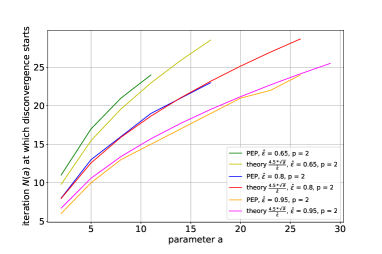
Figure 4: Comparison of theoretical and PEP calculated iteration $N$ after which STM with parameter $a$ starts to disconverge for different $\hat{\varepsilon}$ and $L=1,R=1.$

As one can see PEP and theory are in excellent agreement and the constant $C\sim 4.5$ remains the same from Experiment 1.

Extra Experiment 2.

We check the convergence formula (10) from Theorem 3.1 for $p=2$,

$$f(y^{N})-f(x^{*})\leq O\left(\max\left\{\frac{LR_{0}^{2}}{N^{2}},\frac{\sqrt{\hat{\varepsilon}}LR_{0}^{2}}{\sqrt{N^{3}}},\frac{\hat{\varepsilon}LR_{0}^{2}}{N},\hat{\varepsilon}^{2}LR_{0}^{2}\right\}\right)$$

namely, the level at which the algorithm begins to oscillate after a large number of iterations $N$ with fixed $\hat{\varepsilon}$. To do this, we consider solving maximization problem (8.2) $\tau^{N}=\max_{f}f(y^{N})-f(x^{*})$ setting the parameter $a$ of STM to $\max\left\{1,\sqrt{N\hat{\varepsilon}},N\hat{\varepsilon},N^{2}\hat{\varepsilon}^{2}\right\}$. The theory gives an estimate $LR_{0}^{2}\hat{\varepsilon}^{2}$. Fig. 5 shows the dependence of the maximum difference $\tau^{N}$ on the number of iterations $N$ for different levels of relative noise $\hat{\varepsilon}$ with smoothness constant $L=1$ and initial radius $R=1$.

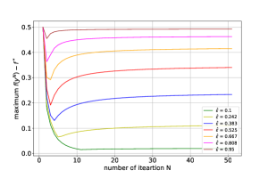
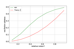
Figure 5: Left: Worst-case results of STM depending on iteration $N$ with optimal $a$ from Theorem 3.1.Right: Theoretical and PEP calculated plateau of oscillation for different relative noise $\hat{\varepsilon}$.

We note that in the results of the PEP and the theory, oscillation of the algorithm around a certain plateau is visible, depending on the relative noise $\hat{\varepsilon}$. However, theoretical estimates do not quite match in order of magnitude to numerical ones.

8.5 Additional experiments for Algorithms 1, 3 and 4.

In this subsection, we show additional experiments connected with Algorithms 1 (ISTM), 3 (AIM) and 4 (AIM with variable $p$), in order to show their efficiency. We run these algorithms with the same setting as described in Section 5.2.

The results of the work of Algorithm ISTM, represented in Fig. 6. These results demonstrate the difference $f(y^{k})-f(x^{*})$ at each iteration of the algorithm, for different values of the parameter $a$.

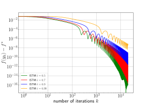
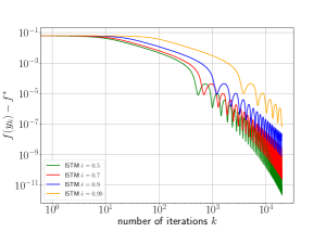
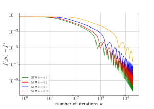
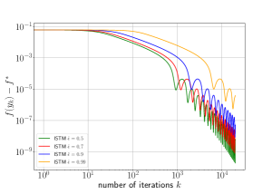
Figure 6: The results of ISTM for for the objective function (45). $a=2$ (up-left), $a=10$ (up-right), $a=20$ (down-left), $a=30$ (down-right).

From Fig. 6, we can see that ISTM will work better when we decrease the value of the parameter $a$. We also note that ISTM always converges for any value of $\hat{\varepsilon}\in[0,1]$. This fact is not satisfied for other algorithms for the class of problems under consideration with relative noise in the gradient. See Vasin et al. [2023], where it was proposed an algorithm that does not converge for $\hat{\varepsilon}\geq 0.712$.

For Algorithms 3 and 4, the results are represented in Fig. 7 and Fig. 8. These results demonstrate the difference $f(y^{k})-f(x^{*})$ at each iteration and theoretical estimate (36). From these figures, we also see that these algorithms always converge for any value of $\hat{\varepsilon}\in[0,1]$. Moreover, from Fig. 7, in the right, we can see the efficiency of the proposed Algorithm 4 (AIM with variable $p$).

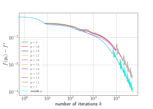
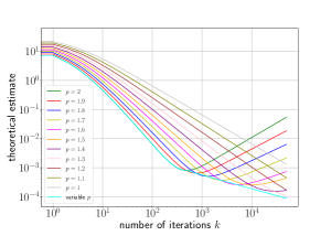
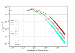
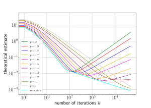
Figure 7: The results of Algorithms 3 and 4, for the objective function (45), with $\hat{\varepsilon}=0.99$ (up), and $\hat{\varepsilon}=0.9$ (down). Here the theoretical estimate is (36).

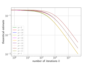
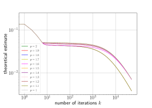
Figure 8: The results of AIM for the objective function (45), with $\hat{\varepsilon}=0.9$ (left) and $\hat{\varepsilon}=0.99$ (right). Here the theoretical estimate is (35).

In the last figure (Fig. 9), we see the results of the comparison between Algorithms 1, 3 and 4, for different values of $a$. From this figure, we can see that Algorithm AIM, will, at the first iterations, work better as the value of $\hat{\varepsilon}$ decreases and the value of $a$ increases. Moreover, the Algorithm AIM gives at the first iterations, a better estimate of a solution to the problem under consideration.

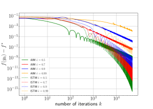
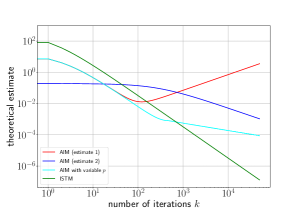
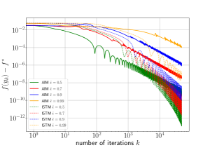
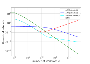
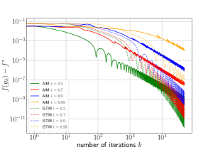
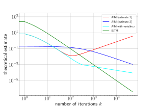
Figure 9: The results of ISTM (Algorithm 1), AIM (Algorithm 3) and AIM with variable $p$ (Algorithm 4) for the objective function (45), with $p=2$ and $a=10,20,30$ from up to down.

References

- Shapiro et al. (2021) Alexander Shapiro, Darinka Dentcheva, and Andrzej Ruszczynski. Lectures on stochastic programming: modeling and theory. SIAM, 2021.
- Baraldi and Kouri (2023) Robert J Baraldi and Drew P Kouri. A proximal trust-region method for nonsmooth optimization with inexact function and gradient evaluations. Mathematical Programming, 201(1-2):559–598, 2023.
- Hintermüller and Stengl (2020) Michael Hintermüller and Steven-Marian Stengl. On the convexity of optimal control problems involving non-linear PDEs or VIs and applications to Nash games. Weierstraß-Institut für Angewandte Analysis und Stochastik Leibniz-Institut …, 2020.
- Matyukhin et al. (2021) Vladislav Matyukhin, Sergey Kabanikhin, Maxim Shishlenin, Nikita Novikov, Artem Vasin, and Alexander Gasnikov. Convex optimization with inexact gradients in hilbert space and applications to elliptic inverse problems. In International Conference on Mathematical Optimization Theory and Operations Research, pages 159–175. Springer, 2021.
- Sabach and Shtern (2017) Shoham Sabach and Shimrit Shtern. A first order method for solving convex bilevel optimization problems. SIAM Journal on Optimization, 27(2):640–660, 2017.
- Solodov (2007) Mikhail Solodov. An explicit descent method for bilevel convex optimization. Journal of Convex Analysis, 14(2):227, 2007.
- Devolder et al. (2013) Olivier Devolder, François Glineur, Yurii Nesterov, et al. Intermediate gradient methods for smooth convex problems with inexact oracle. Technical report, Technical report, CORE-2013017, 2013.
- Polyak (1987) Boris T Polyak. Introduction to optimization. 1987.
- Stonyakin et al. (2021) Fedor Stonyakin, Alexander Tyurin, Alexander Gasnikov, Pavel Dvurechensky, Artem Agafonov, Darina Dvinskikh, Mohammad Alkousa, Dmitry Pasechnyuk, Sergei Artamonov, and Victorya Piskunova. Inexact model: A framework for optimization and variational inequalities. Optimization Methods and Software, 36(6):1155–1201, 2021.
- Vasin et al. (2023) Artem Vasin, Alexander Gasnikov, Pavel Dvurechensky, and Vladimir Spokoiny. Accelerated gradient methods with absolute and relative noise in the gradient. Optimization Methods and Software, pages 1–50, 2023.
- Granichin and Polyak (2003) ON Granichin and BT Polyak. Randomizirovannye algoritmy otsenivaniya i optimizatsii pri pochti proizvol’nykh pomekhakh. Nauka, 2003.
- Nemirovski (1986) Arkadi S Nemirovski. Regularizing properties of the conjugate gradient method for ill-posed problems. Zhurnal Vychislitel’noi Matematiki i Matematicheskoi Fiziki, 26(3):332–347, 1986.
- Devolder et al. (2014) Olivier Devolder, François Glineur, and Yurii Nesterov. First-order methods of smooth convex optimization with inexact oracle. Mathematical Programming, 146:37–75, 2014.
- d’Aspremont (2008) Alexandre d’Aspremont. Smooth optimization with approximate gradient. SIAM Journal on Optimization, 19(3):1171–1183, 2008.
- Cohen et al. (2018) Michael Cohen, Jelena Diakonikolas, and Lorenzo Orecchia. On acceleration with noise-corrupted gradients. In International Conference on Machine Learning, pages 1019–1028. PMLR, 2018.
- Gorbunov et al. (2019) Eduard Gorbunov, Darina Dvinskikh, and Alexander Gasnikov. Optimal decentralized distributed algorithms for stochastic convex optimization. arXiv preprint arXiv:1911.07363, 2019.
- Khanh et al. (2023) Pham Duy Khanh, Boris Mordukhovich, and Dat Ba Tran. Inexact proximal methods for weakly convex functions. arXiv preprint arXiv:2307.15596, 2023.
- Poljak (1981) BT Poljak. Iterative algorithms for singular minimization problems. In Nonlinear Programming 4, pages 147–166. Elsevier, 1981.
- Gannot (2022) Oran Gannot. A frequency-domain analysis of inexact gradient methods. Mathematical Programming, 194(1-2):975–1016, 2022.
- Drusvyatskiy and Xiao (2023) Dmitriy Drusvyatskiy and Lin Xiao. Stochastic optimization with decision-dependent distributions. Mathematics of Operations Research, 48(2):954–998, 2023.
- Kotsalis et al. (2022) Georgios Kotsalis, Guanghui Lan, and Tianjiao Li. Simple and optimal methods for stochastic variational inequalities, i: operator extrapolation. SIAM Journal on Optimization, 32(3):2041–2073, 2022.
- Dvurechensky et al. (2018) Pavel Dvurechensky, Alexander Gasnikov, and Alexey Kroshnin. Computational optimal transport: Complexity by accelerated gradient descent is better than by Sinkhorn’s algorithm. In Jennifer Dy and Andreas Krause, editors, Proceedings of the 35th International Conference on Machine Learning, volume 80 of Proceedings of Machine Learning Research, pages 1367–1376, 2018. arXiv:1802.04367.
- d’Aspremont et al. (2021) Alexandre d’Aspremont, Damien Scieur, Adrien Taylor, et al. Acceleration methods. Foundations and Trends® in Optimization, 5(1-2):1–245, 2021.
- Gasnikov and Nesterov (2018) Alexander Vladimirovich Gasnikov and Yu E Nesterov. Universal method for stochastic composite optimization problems. Computational Mathematics and Mathematical Physics, 58:48–64, 2018.
- Dvurechensky and Gasnikov (2016) Pavel Dvurechensky and Alexander Gasnikov. Stochastic intermediate gradient method for convex problems with stochastic inexact oracle. Journal of Optimization Theory and Applications, 171:121–145, 2016.
- Kamzolov et al. (2021) Dmitry Kamzolov, Pavel Dvurechensky, and Alexander V Gasnikov. Universal intermediate gradient method for convex problems with inexact oracle. Optimization Methods and Software, 36(6):1289–1316, 2021.
- Goujaud et al. (2022) Baptiste Goujaud, Céline Moucer, François Glineur, Julien Hendrickx, Adrien Taylor, and Aymeric Dieuleveut. Pepit: computer-assisted worst-case analyses of first-order optimization methods in python. arXiv preprint arXiv:2201.04040, 2022.
- Taylor et al. (2017) Adrien B Taylor, Julien M Hendrickx, and François Glineur. Smooth strongly convex interpolation and exact worst-case performance of first-order methods. Mathematical Programming, 161:307–345, 2017.
- Gasnikov and Nesterov (2016) Alexander Gasnikov and Yurii Nesterov. Universal fast gradient method for stochastic composit optimization problems. arXiv preprint arXiv:1604.05275, 2016.
- Gorbunov et al. (2021) Eduard Gorbunov, Marina Danilova, Innokentiy Shibaev, Pavel Dvurechensky, and Alexander Gasnikov. Near-optimal high probability complexity bounds for non-smooth stochastic optimization with heavy-tailed noise. arXiv preprint arXiv:2106.05958, 2021.
- De Klerk et al. (2017) Etienne De Klerk, François Glineur, and Adrien B Taylor. On the worst-case complexity of the gradient method with exact line search for smooth strongly convex functions. Optimization Letters, 11:1185–1199, 2017.
- Drori and Teboulle (2014) Yoel Drori and Marc Teboulle. Performance of first-order methods for smooth convex minimization: a novel approach. Mathematical Programming, 145(1-2):451–482, 2014.
- ApS (2019) Mosek ApS. Mosek optimization toolbox for matlab. User’s Guide and Reference Manual, Version, 4:1, 2019.
- Nesterov (2018) Yurii Nesterov. Lectures on convex optimization, volume 137. Springer, 2018.
- Taylor and Drori (2023) Adrien Taylor and Yoel Drori. An optimal gradient method for smooth strongly convex minimization. Mathematical Programming, 199(1-2):557–594, 2023.
- Gorbunov et al. (2020) Eduard Gorbunov, Marina Danilova, and Alexander Gasnikov. Stochastic optimization with heavy-tailed noise via accelerated gradient clipping. Advances in Neural Information Processing Systems, 33:15042–15053, 2020.