It HAS to be Subjective: Human Annotator Simulation via Zero-shot Density Estimation

Abstract

Human annotator simulation (HAS) serves as a cost-effective substitute for human evaluation such as data annotation and system assessment. Human perception and behaviour during human evaluation exhibit inherent variability due to diverse cognitive processes and subjective interpretations, which should be taken into account in modelling to better mimic the way people perceive and interact with the world. This paper introduces a novel meta-learning framework that treats HAS as a zero-shot density estimation problem, which incorporates human variability and allows for the efficient generation of human-like annotations for unlabelled test inputs. Under this framework, we propose two new model classes, conditional integer flows and conditional softmax flows, to account for ordinal and categorical annotations, respectively. The proposed method is evaluated on three real-world human evaluation tasks and shows superior capability and efficiency to predict the aggregated behaviours of human annotators, match the distribution of human annotations, and simulate the inter-annotator disagreements.

1 Introduction

Human evaluation is fundamental to machine learning research, guiding processes such as data annotation and model assessment, which for instance include perceptual quality evaluation of synthesized speech, text, and image (Ma et al., 2015; Patton et al., 2016; wei Fu et al., 2018; Talebi & Milanfar, 2018; Lo et al., 2019; Borade & Netak, 2020; Ramesh & Sanampudi, 2022), annotation generation for weak supervision (Ratner et al., 2016; Wu et al., 2022a), and model optimization based on human preference (Schatzmann et al., 2007; Asri et al., 2016; Gür et al., 2018; Ruiz et al., 2019; Shi et al., 2019; Lin et al., 2021). Collecting human annotations or evaluations often requires substantial resources and may expose human annotators to distressing and harmful content in sensitive tasks (e.g., toxic speech detection, suicidal risk prediction, and depression detection). This inspires the exploration of human annotator simulation (HAS) as a scalable and cost-effective alternative, which facilitates large-scale dataset evaluation, benchmarking, and system comparisons.

Variability is a unique aspect of real-world human evaluation, since individual variations in cognitive biases, cultural backgrounds, and personal experiences (Hirschberg et al., 2003; Wiebe et al., 2004; Haselton et al., 2015) can lead to variability in human interpretation (Lotfian & Busso, 2019; Mathew et al., 2021; Maniati et al., 2022). HAS aims to incorporate the variability present in human evaluation rather than solely relying on majority opinions, which mitigates potential biases and over-representation in scenarios where dominant opinions could potentially overshadow minority viewpoints (Dixon et al., 2018; Hutchinson et al., 2020), thus promoting fairness and inclusivity.

In this work, we investigate HAS for the automatic generation of human-like annotations that take into account the variability in human evaluation. A novel meta-learning framework that treats HAS as a zero-shot density estimation problem is introduced, which allows for the efficient generation of human-like annotations for unlabelled test inputs. Under this framework, two new model classes, conditional integer flows and conditional softmax flows, are proposed to account for ordinal and categorical annotations respectively, which are common types of annotations in human evaluation tasks. The proposed method shows superior capability and efficiency to predict the aggregated behaviours of human annotators, match the distribution of human annotations, and simulate the level of inter-annotator agreement on three real-world human evaluation tasks: emotion recognition, toxic speech detection, and speech quality assessment.

2 Human Annotator Simulation (HAS)

2.1 The Variability in Human Evaluation is Valuable

Each individual’s perception of the world is unique and influenced by their physical state and cognitive biases, which leads to diverse and subjective interpretations (see Appendix A for more detail). Such subjectivity can be manifest in various tasks such as emotion recognition (Hirschberg et al., 2003; Mihalcea & Liu, 2006), perceptual quality assessment (Wiebe et al., 2004; Seshadrinathan et al., 2010; Zen & Vanderdonckt, 2016), and user experience evaluation (Zen & Vanderdonckt, 2016). It has been argued that achieving a deterministic “ground truth” in subjective tasks like human evaluation is not feasible, nor essential  (Alm, 2011; Wu et al., 2022b). Therefore, we advocate for methodologies that focus on modelling annotators’ subjective interpretations, rather than seek to reduce the variability in annotations: instead of only predicting the majority opinion, it is important to account for the human perception variability when designing a human annotator simulator. The following are three examples that demonstrate the importance of modelling variability in HAS:

Revealing data ambiguity. Incorporating the variability in human perception empowers HAS to reveal potential ambiguity or complexity in data, providing valuable insights for further analysis.

Mitigating bias and over-representation. Incorporating the variability in human judgements prevents HAS from being biased towards a certain perspective and ignoring minority viewpoints, leading to a more inclusive representation of opinions where all viewpoints are given due consideration.

Improving model alignment. Optimization based on human feedback has led to superior performance on tasks such as text generation (Christiano et al., 2017; Ouyang et al., 2022; Rafailov et al., 2023), which aligns the behaviour of language models with human preferences. HAS could be helpful in this task, as it is an efficient and cost-effective alternative to generating human feedback.

2.2 Problem Formulation and Related Work

HAS involves modelling a dataset $\mathcal{D}=\{({\bm{x}}_{i},{\bm{\eta}}_{i}^{(1)},\cdots,{\bm{\eta}}_{i}^{(M_{i})})\}_{i=1}^{N}$ from human evaluation, where each data point is a tuple of an input ${\bm{x}}_{i}$ and its corresponding labels ${\bm{\eta}}_{i}^{(1)},\cdots,{\bm{\eta}}_{i}^{(M_{i})}$ provided by $M_{i}$ independent human annotators. Note that different inputs may be labelled by different sets of annotators. HAS aims to model the conditional annotation distribution ${\textnormal{p}}({\bm{\eta}}|{\bm{x}})$ in order to simulate human-like annotations ${\bm{\eta}}_{*}^{(1)},\cdots,{\bm{\eta}}_{*}^{(M_{*})}$ for any unseen input ${\bm{x}}_{*}$ in a way that reflects how it would be labelled by human annotators. Prior work mainly investigated two approaches to this problem.

The first approach uses a single proxy variable ${\bm{\eta}}_{i}$ (e.g., majority vote or average score) to summarize all annotations for each input ${\bm{x}}_{i}$ (Kim et al., 2013; Djuric et al., 2015; Patton et al., 2016; Poria et al., 2017). This creates a proxy dataset $\mathcal{D}^{\prime}=\{({\bm{x}}_{i},{\bm{\eta}}_{i})\}_{i=1}^{N}$ and converts HAS into a supervised learning problem, which is usually solved by fitting a discriminative model to estimate the conditional distribution for the proxy variable. This approach assumes that each input ${\bm{x}}_{i}$ has only one ground-truth label ${\bm{\eta}}_{i}$, and thus the conditional distribution only quantifies the uncertainty due to noisy observation and lack of training examples. Clearly, modelling a single proxy variable as in this approach fails to take into account the subjectivity and diversity in human behaviour and perception and thus will result in an underestimate of variability in the simulated annotations. Other work incorporated the variance of human annotations into the proxy variable (Deng et al., 2012; Prabhakaran et al., 2012; Plank et al., 2014; Dang et al., 2017; Han et al., 2017; Leng et al., 2021). However, all these approaches still focus on obtaining the “correct” label (e.g., aiming for improved prediction accuracy) and minimizing the discrepancy among annotators (e.g., reducing “noise” in annotations) rather than embracing inter-annotator disagreements.

The second approach explicitly models the behaviour of different annotators using different individual models in an ensemble or different heads in a single model (Fayek et al., 2016; Chou & Lee, 2019; Davani et al., 2022). However, this approach is computationally feasible only when the number of annotators is relatively small and when a sufficient quantity of annotation is available for each annotator, which can then not be applied to large crowd-sourced datasets, such as Lotfian & Busso (2019); Mathew et al. (2021); Maniati et al. (2022), which are common in real-world applications.

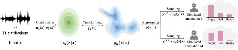
Figure 1: Diagram for the proposed zero-shot human annotator simulation framework.

3 Human Annotator Simulation via Zero-shot Density Estimation

3.1 A Meta-learning Framework for Zero-shot Human Annotator Simulation

We propose a novel meta-learning framework for HAS to address the issues in prior work, where the collection of all human annotations for each input ${\bm{x}}_{i}$ is viewed as a dataset $\mathcal{D}_{i}=\{{\bm{\eta}}_{i}^{(m)}\}_{m=1}^{M_{i}}$. This framework transforms HAS into a density estimation problem for the human annotation of each input ${\bm{x}}_{i}$ given samples from $\mathcal{D}_{i}$. We propose to meta-learn a density estimator across all datasets $\mathcal{D}_{\text{meta}}=\{\mathcal{D}_{i}\}_{i=1}^{N}$, in order to leverage knowledge about the agreements and disagreements among different human annotators across different examples. This formulates a zero-shot density estimation problem, since there is no human annotation available for test-time adaptation except for a “descriptor” (i.e., the test input) ${\bm{x}}_{*}$. In other words, the meta-learned density estimator should allow efficient sampling of human-like annotations and their likelihoods evaluations for any unseen input ${\bm{x}}_{*}$ without access to any samples for the ground-truth human annotations of ${\bm{x}}_{*}$.

In this work, the meta-learning framework is realized using a latent variable model:

$${\textnormal{p}}_{{\bm{\theta}}}({\bm{y}}|{\bm{x}})=\int{\textnormal{p}}({\bm{y}}|{\bm{v}}){\textnormal{p}}_{{\bm{\phi}}}({\bm{v}}|{\bm{z}}){\textnormal{p}}_{{\bm{\Lambda}}}({\bm{z}}|{\bm{x}})d{\bm{v}}d{\bm{z}},$$ (1)

where the conditional prior ${\textnormal{p}}_{{\bm{\Lambda}}}({\bm{z}}|{\bm{x}})$ learns to summarize useful information about ${\bm{x}}$ and encode the possible disagreements over ${\bm{x}}$ among different human annotators, which is helpful for the likelihood ${\textnormal{p}}_{{\bm{\phi}}}({\bm{y}}|{\bm{z}})=\int{\textnormal{p}}({\bm{y}}|{\bm{v}}){\textnormal{p}}_{{\bm{\phi}}}({\bm{v}}|{\bm{z}})d{\bm{v}}$ to simulate human-like annotations.

Figure 1 illustrates the proposed framework workflow. Specifically, the conditional prior is modelled by a conditional factorized Gaussian distribution ${\textnormal{p}}_{\bm{\Lambda}}({\bm{z}}|{\bm{x}})=\mathcal{N}({\bm{z}}|{\bm{\mu}}_{\bm{\Lambda}}({\bm{x}}),{\operatorname{diag}}({\bm{\sigma}}_{\bm{\Lambda}}^{2}({\bm{x}})))$ whose mean ${\bm{\mu}}_{\bm{\Lambda}}({\bm{x}})$ and variance ${\bm{\sigma}}_{\bm{\Lambda}}^{2}({\bm{x}})$ are parameterized by a neural network with parameters ${\bm{\Lambda}}$. The intermediate variable ${\bm{v}}$ is obtained by a deterministic invertible transformation ${\textnormal{p}}_{{\bm{\phi}}}({\bm{v}}|{\bm{z}})=\delta({\bm{v}}-{\bm{f}}_{{\bm{\phi}}}({\bm{z}}))$, where ${\bm{f}}_{{\bm{\phi}}}({\bm{z}})$ is parameterized by an invertible neural network with parameters ${\bm{\phi}}$, and $\delta(\cdot)$ is the multivariate Dirac delta function. This results in a conditional normalizing flow (CNF):

$${\textnormal{p}}_{\bm{\theta}}({\bm{v}}|{\bm{x}})=\int\delta({\bm{v}}-{\bm{f}}_{{\bm{\phi}}}({\bm{z}})){\textnormal{p}}_{{\bm{\Lambda}}}({\bm{z}}|{\bm{x}})d{\bm{z}}={\textnormal{p}}_{\bm{\Lambda}}\left.\left({\bm{f}}^{-1}_{\bm{\phi}}({\bm{v}})\right|{\bm{x}}\right)\left|\operatorname{det}\left(\frac{\partial{\bm{f}}^{-1}_{\bm{\phi}}({\bm{v}})}{\partial{\bm{v}}}\right)\right|,$$ (2)

where $\operatorname{det}(\cdot)$ denotes the determinant operator, ${\partial{\bm{f}}^{-1}_{\bm{\phi}}({\bm{v}})}/{\partial{\bm{v}}}$ denotes the Jacobin matrix of ${\bm{f}}^{-1}_{\bm{\phi}}({\bm{v}})$, and ${\bm{\theta}}\coloneqq\{{\bm{\phi}},{\bm{\Lambda}}\}$ denotes all parameters in this base CNF. This modelling choice has the advantage of having tractable marginal likelihood as in Eqn. (2) while not restricting the intermediate variable ${\bm{v}}$ to a specific type of distribution as in previous methods, e.g., Gaussian (Han et al., 2017) and Student-t  (Wu et al., 2023) distributions, thus offering enhanced tractability, flexibility and generality. In addition, samples can be efficiently drawn from this model by first drawing ${\bm{z}}\sim{\textnormal{p}}_{{\bm{\Lambda}}}({\bm{z}}|{\bm{x}})$ from the conditional prior and then computing the deterministic flow transformation ${\bm{v}}={\bm{f}}_{{\bm{\phi}}}({\bm{z}})$.

Finally, the output variable ${\bm{y}}$ is obtained by augmenting the intermediate variable ${\bm{v}}$ using the transformation ${\textnormal{p}}({\bm{y}}|{\bm{v}})$, in order to accommodate different types of annotation. For continuous annotations, the identity transformation ${\textnormal{p}}({\bm{y}}|{\bm{v}})=\delta({\bm{y}}-{\bm{v}})$ is used, which exactly recovers the base CNF model. However, real-world human evaluation tasks often involve discrete annotations that are either ordinal or categorical. In the following sections, two new model classes with meta-learning objectives are introduced to accommodate these annotation types.

3.2 Meta-learning Conditional Integer Flows for Ordinal Annotations

Modelling. Discrete ordinal annotations are often used in K-point rating systems, where the ratings are integer-valued with a clear ordering. We propose a new class of models called conditional integer flows (I-CNFs), which augment the base CNFs by quantizing the continuous intermediate variable $v$ to its nearest integer by using a rounding transformation ${\textnormal{p}}(y|v)=\mathbb{I}(y-\nicefrac{{1}}{{2}}<v\leq y+\nicefrac{{1}}{{2}})$, where $\mathbb{I}(\cdot)$ is the indicator function. Let $o$ be an ordinal variable that represents the ordinal human rating for an input ${\bm{x}}$. The marginal likelihood of I-CNF is given by

$${\textnormal{p}}_{{\bm{\theta}}}(o=y|{\bm{x}})=\int_{-\infty}^{\infty}\mathbb{I}(y-\nicefrac{{1}}{{2}}<v\leq y+\nicefrac{{1}}{{2}}){\textnormal{p}}_{{\bm{\theta}}}(v|{\bm{x}})dv=\int_{y-\nicefrac{{1}}{{2}}}^{y+\nicefrac{{1}}{{2}}}{\textnormal{p}}_{{\bm{\theta}}}(v|{\bm{x}})dv,$$ (3)

where ${\textnormal{p}}_{{\bm{\theta}}}(v|{\bm{x}})$ is the marginal likelihood of the base CNF defined in Eqn. (2). Since the marginal likelihood of I-CNF given in Eqn. (3) is analytically intractable due to the rounding transformation, we propose to approximate it using numerical integration. In practice, the rectangular rule is found to work well in terms of both performance and efficiency in this setting, where the density of ${\textnormal{p}}_{{\bm{\theta}}}(v|{\bm{x}})$ within the interval $v\in(y-\nicefrac{{1}}{{2}},y+\nicefrac{{1}}{{2}}]$ is approximated by the midpoint density value:

$$\int_{y-\nicefrac{{1}}{{2}}}^{y+\nicefrac{{1}}{{2}}}{\textnormal{p}}_{{\bm{\theta}}}(v|{\bm{x}})dv\approx\left(\left(y+\frac{1}{2}\right)-\left(y-\frac{1}{2}\right)\right)\cdot{\textnormal{p}}_{{\bm{\theta}}}\left(\left.\frac{(y-\nicefrac{{1}}{{2}})+(y+\nicefrac{{1}}{{2}})}{2}\right|{\bm{x}}\right)={\textnormal{p}}_{{\bm{\theta}}}(y|{\bm{x}}).$$ (4)

This means that Eqn. (2) can be used as a proxy to evaluate the likelihood of I-CNF.

Meta-learning. Using the numerical approximation given in Eqn. (4), the loss $\mathcal{L}({\bm{\theta}};\mathcal{D}_{i},{\bm{x}}_{i})$ for I-CNF on a single dataset $\mathcal{D}_{i}$ can be defined as the average negative log marginal likelihood of Eqn. (2) evaluated on the human annotations $\mathcal{D}_{i}=\{\eta_{i}^{(m)}\}_{m=1}^{M_{i}}$ given the corresponding input ${\bm{x}}_{i}$:

$$\begin{split}\mathcal{L}({\bm{\theta}};\mathcal{D}_{i},{\bm{x}}_{i})&=-\frac{1}{M_{i}}\sum_{m=1}^{M_{i}}\left(\log{\textnormal{p}}_{\bm{\Lambda}}\left.\left(f^{-1}_{\bm{\phi}}(\eta_{i}^{(m)})\right|{\bm{x}}_{i}\right)+\log\left|\operatorname{det}\left(\frac{\partial f^{-1}_{\bm{\phi}}(\eta_{i}^{(m)})}{\partial\eta_{i}^{(m)}}\right)\right|\right).\end{split}$$ (5)

Following the episodic training scheme (Vinyals et al., 2016; Snell et al., 2017; Chen et al., 2023), we treat density estimation on each dataset as a learning problem and randomly sample a subset of such learning problems to train on at each step during meta-training. This results in a meta-learning objective across all datasets $\mathcal{D}_{\text{meta}}$:

$$\mathcal{L}_{\text{meta}}({\bm{\theta}};\mathcal{D}_{\text{meta}},\{{\bm{x}}_{i}\}_{i=1}^{N})=\mathbb{E}_{D_{i}\sim{\textnormal{p}}(\mathcal{D})}[\mathcal{L}({\bm{\theta}};\mathcal{D}_{i},{\bm{x}}_{i})],$$ (6)

where ${\textnormal{p}}(\mathcal{D})$ denotes the uniform distribution over the datasets in $\mathcal{D}_{\text{meta}}$. Intuitively, this objective maps all human annotation to the latent space of their corresponding input by the inverse flow transformation $z_{i}^{(m)}=f^{-1}_{\bm{\phi}}(\eta_{i}^{(m)})$ during meta-training, which helps the model to build a diverse latent representation that captures the variability in human annotations across different inputs. At test time, the I-CNF can simulate human-like annotations for an unseen, unlabelled input ${\bm{x}}_{*}$ by first drawing $v_{*}^{(m)}\sim{\textnormal{p}}_{{\bm{\theta}}}(v|{\bm{x}}_{*})$ from the base CNF then applying the rounding function $y_{*}^{(m)}=\lfloor v_{*}^{(m)}\rfloor$, for $m=1,\cdots,M_{*}$, where $M_{*}$ denotes the number of annotations to be simulated.

3.3 Meta-learning Conditional Softmax Flows for Categorical Annotations

Modelling. To account for non-ordinal categorical annotations (e.g., emotion categories), we propose a new class of models called conditional softmax flows (S-CNFs), which augments the base CNFs by applying the softmax function ${\textnormal{p}}({\bm{y}}|{\bm{v}})=\delta\left({\bm{y}}-\mathrm{softmax}({\bm{v}})\right)$ to transform the continuous intermediate variable ${\bm{v}}$ into categorical probabilities ${\bm{y}}$. Let $c$ be a categorical variable with probability ${\textnormal{P}}(c=k|{\bm{y}})={\bm{y}}_{k}~{}(k=1,\cdots,K)$ that represents the categorical human annotation for an input ${\bm{x}}$, with ${\textnormal{P}}(c=k|{\bm{v}})=\int{\bm{y}}_{k}\delta\left({\bm{y}}-\mathrm{softmax}({\bm{v}})\right)d{\bm{y}}=\mathrm{softmax}({\bm{v}})_{k}$. The marginal likelihood of S-CNF is given by

$${\textnormal{P}}_{\bm{\theta}}(c=k|{\bm{x}})=\int{\textnormal{P}}(c=k|{\bm{v}}){\textnormal{p}}_{{\bm{\theta}}}({\bm{v}}|{\bm{x}})d{\bm{v}}=\int\mathrm{softmax}({\bm{v}})_{k}{\textnormal{p}}_{{\bm{\theta}}}({\bm{v}}|{\bm{x}})d{\bm{v}},$$ (7)

where ${\textnormal{p}}_{{\bm{\theta}}}({\bm{v}}|{\bm{x}})$ is the marginal likelihood of the base CNF defined in Eqn. (2). Since the marginal likelihood of the S-CNF given in Eqn. (7) is analytically intractable due to the softmax transformation, we propose to approximate it using variational inference (Wainwright et al., 2008) with a learnable mean-field Gaussian variational posterior ${\textnormal{q}}_{\bm{\Omega}}({\bm{v}}|{\bm{y}})=\mathcal{N}({\bm{v}}|{\bm{\mu}}_{\bm{\Omega}}({\bm{y}}),{\operatorname{diag}}({\bm{\sigma}}_{\bm{\Omega}}^{2}({\bm{y}})))$, which can be seen as a probabilistic inverse of the softmax transformation ${\textnormal{p}}({\bm{y}}|{\bm{v}})$. Applying Jensen’s inequality to the log marginal likelihood of the S-CNF in Eqn. (7), a tractable evidence lower bound (ELBO) is obtained:

$$\log{\textnormal{P}}_{\bm{\theta}}(c=k|{\bm{x}})\geq\mathds{E}_{{\textnormal{q}}_{\bm{\Omega}}({\bm{v}}|{\bm{y}})}\left[\log{\textnormal{P}}(c=k|{\bm{v}})+\log{\textnormal{p}}_{\bm{\theta}}({\bm{v}}|{\bm{x}})-\log{\textnormal{q}}_{\bm{\Omega}}({\bm{v}}|{\bm{y}})\right].$$ (8)

It is worth noting that the softmax flow likelihood ${\textnormal{P}}(c=k|{\bm{v}})=\mathrm{softmax}({\bm{v}})_{k}$ places non-zero probability mass for every category $k=1,\cdots,K$, which is different from argmax flow (Hoogeboom et al., 2021) whose likelihood only places probability mass for a single category. From a modelling perspective, softmax flow has a better capacity to represent the variability and uncertainty in human annotations. From an optimization perspective, the ELBO for softmax flow is always well-defined, whereas the ELBO for argmax flow is not defined when the model output does not match the human annotation, for which the reason lies in the fact that the log-likelihood would be $\log(0)$ in this case, which requires additional thresholding tricks to fix (Hoogeboom et al., 2021).

Meta-learning. Using the variational approximation defined in Eqn. (8), the loss $\mathcal{L}({\bm{\theta}},{\bm{\Omega}};\mathcal{D}_{i},{\bm{x}}_{i})$ for S-CNF on a single dataset $\mathcal{D}_{i}$ can be defined as the average negative ELBO evaluated on the human annotations $\mathcal{D}_{i}=\{{\bm{\eta}}_{i}^{(m)}\}_{m=1}^{M_{i}}$ given the corresponding input ${\bm{x}}_{i}$:

$$\mathcal{L}({\bm{\theta}},{\bm{\Omega}};\mathcal{D}_{i},{\bm{x}}_{i})=-\frac{1}{M_{i}}\sum_{m=1}^{M_{i}}\mathbb{E}_{{\textnormal{q}}_{\bm{\Omega}}({\bm{v}}|{\bm{\eta}}_{i}^{(m)})}\left[\sum_{k=1}^{K}{\bm{\eta}}_{i,k}^{(m)}\log{\textnormal{P}}(c_{i}=k|{\bm{v}})+\log{\textnormal{p}}_{\bm{\theta}}({\bm{v}}|{\bm{x}}_{i})-\log{\textnormal{q}}_{\bm{\Omega}}({\bm{v}}|{\bm{\eta}}_{i}^{(m)})\right],$$ (9)

where the expectation over the variational posterior is approximated by Monte Carlo simulation with the reparameterization trick (Kingma & Welling, 2014). As in Section 3.2, we follow the episodic training scheme with a meta-learning objective $\mathcal{L}({\bm{\theta}},{\bm{\Omega}};\mathcal{D}_{\text{meta}},\{{\bm{x}}_{i}\}_{i=1}^{N})=\mathbb{E}_{D_{i}\sim{\textnormal{p}}(\mathcal{D})}[\mathcal{L}({\bm{\theta}},{\bm{\Omega}};\mathcal{D}_{i},{\bm{x}}_{i})]$ for meta-training and use a similar flow sampling scheme but apply the softmax function ${\bm{y}}_{*}^{(m)}=\mathrm{softmax}({\bm{v}}_{*}^{(m)})$ to the samples ${\bm{v}}_{*}^{(m)}$ from the base CNF at test time. Note that each sample of S-CNF is a categorical distribution with probabilities ${\bm{y}}_{*}^{(m)}$.

4 Evaluation Metrics

Several metrics are adopted to measure the empirical performance of HAS in terms of mean/majority prediction, distribution matching, and human variability simulation.

Mean/majority prediction. For ordinal annotations, the root mean squared error is used to evaluate the quality of the mean prediction for all test inputs: $\text{RMSE}^{\bar{y}}=\sqrt{\frac{1}{N}\sum_{i=1}^{N}(\bar{y}_{i}-\bar{\eta}_{i})^{2}}$, where $\bar{y}_{i}=\frac{1}{M_{*}}\sum_{m=1}^{M_{*}}y_{i}^{(m)}$ and $\bar{\eta}_{i}=\frac{1}{M_{i}}\sum_{m=1}^{M_{i}}\eta_{i}^{(m)}$. For categorical annotations, the classification accuracy (Acc) for the majority vote is evaluated for all test inputs that have majority human annotations.

Distribution matching. The negative log likelihood (NLL) is used to evaluate how well the model estimates the human annotation distribution: $\text{NLL}^{\text{all}}=-\frac{1}{N}\sum_{i=1}^{N}\left(\frac{1}{M_{i}}\sum_{m=1}^{M_{i}}\log{\textnormal{p}}_{\bm{\theta}}({\bm{\eta}}_{i}^{(m)}|{\bm{x}}_{i})\right)$.

Inter-annotator disagreement simulation. Apart from evaluating the goodness of fit, additional metrics are adopted to explicitly measure how well the model simulates the variability and disagreements in human annotations: 1) the root mean squared error of the standard deviations of the annotations for all test inputs: $\text{RMSE}^{s}=\sqrt{\frac{1}{N}\sum_{i=1}^{N}\left(\sigma_{i}-s_{i}\right)^{2}}$, where $\sigma_{i}=\sqrt{\frac{1}{M_{i}}\sum_{m=1}^{M_{i}}(\eta_{i}^{(m)}-\bar{\eta}_{i})^{2}}$ and $s_{i}=\sqrt{\frac{1}{M_{*}}\sum_{m=1}^{M_{*}}(y_{i}^{(m)}-\bar{y}_{i})^{2}}$ for ordinal annotations, and $\sigma_{i}=\frac{1}{K}\sum_{k=1}^{K}\sqrt{\frac{1}{M_{i}}\sum_{m=1}^{M_{i}}(\eta_{i,k}^{(m)}-\bar{\eta}_{i,k})^{2}}$ and $s_{i}=\frac{1}{K}\sum_{k=1}^{K}\sqrt{\frac{1}{M_{*}}\sum_{m=1}^{M_{*}}(y_{i,k}^{(m)}-\bar{y}_{i,k})^{2}}$ for categorical annotations, and 2) the absolute error of the average standard deviations of the annotations for all test inputs: $\mathcal{E}(\bar{s})=|\bar{\sigma}-\bar{s}|$, where $\bar{\sigma}=\sum_{i=1}^{N}\sigma_{i}$ and $\bar{s}=\sum_{i=1}^{N}s_{i}$. For categorical annotations, Fleiss’s kappa ($\kappa$) (Fleiss, 1971) is additionally adopted to measure the inter-annotator disagreements, where $\kappa$ is a real number between $-1$ and $+1$, with $-1$ indicating no observed agreement and $+1$ indicating perfect agreement. The absolute error between the kappas of human annotations ($\kappa$) and simulated annotations ($\hat{\kappa}$) for all test inputs is reported: $\mathcal{E}(\hat{\kappa})=|\hat{\kappa}-\kappa|$.

5 Experiments

Setup. The proposed meta-learned zero-shot density estimation method for HAS from Section 3 is evaluated by three representative real-world human evaluation tasks for speech and natural language processing: emotion category annotation, toxic speech detection, and speech quality assessment. The results are reported using evaluation metrics defined in Section 4 and several representative examples are visualized, which demonstrate the superior capability of the proposed method to capture the aggregated behaviours of human annotators, match the distribution of human annotations, and simulate the variability and disagreement of human perception and interpretation.

Baselines. The proposed I-CNF and S-CNF are compared to baselines of various types such as ensemble methods, Bayesian methods, and conditional generative models. This includes deep ensemble (Ensemble) (Lakshminarayanan et al., 2017), Monte-Carlo dropout (MCDP) (Gal & Ghahramani, 2016), Bayes-by-backprop (BBB) (Blundell et al., 2015), conditional variational autoencoder (CVAE) (Kingma & Welling, 2014), conditional argmax flow (A-CNF) (Hoogeboom et al., 2021), Dirichlet prior network (DPN) (Malinin & Gales, 2018), Gaussian process (GP) (Williams & Rasmussen, 2006), and evidential deep learning (EDL) (Amini et al., 2020). We fit them to all available human annotations for all utterances in the training set, tune hyperparameters on the validation set, and report performance on the test set. $M_{*}=100$ samples are used to compute evaluation metrics at test time. The Ensemble only consists of 10 systems due to its expensive computational cost.

Backbone architecture. The same neural network feature encoder is used in all compared methods to extract features from inputs, which follows an upstream-downstream paradigm. The upstream model, also called a foundation model (Bommasani et al., 2021), is pre-trained on a large amount of unlabelled data to learn universal representations. WavLM (Chen et al., 2022) and RoBERTa (Liu et al., 2019) are used as the pre-trained upstream models for speech and text inputs, respectively. The downstream model consists of two Transformer encoder blocks followed by two fully connected (FC) layers, which are fine-tuned to target specific applications.

Table 1: Test performance on the emotion category annotation task. CVAE collapses to one category for all inputs.

	Acc$~{}(\uparrow)$	$\text{NLL}^{\text{all}}~{}(\downarrow)$	$\text{RMSE}^{s}~{}(\downarrow)$	$\mathcal{E}(\bar{s})~{}(\downarrow)$	$\mathcal{E}(\hat{\kappa})~{}(\downarrow)$
MCDP	0.582$\pm$0.003	1.423$\pm$0.012	0.294$\pm$0.001	0.193$\pm$0.000	0.467$\pm$0.005
Ensemble	0.603$\pm$0.002	1.458$\pm$0.004	0.271$\pm$0.003	0.160$\pm$0.004	0.344$\pm$0.017
BBB	0.565$\pm$0.010	1.459$\pm$0.011	0.289$\pm$0.005	0.187$\pm$0.008	0.511$\pm$0.034
DPN	0.581$\pm$0.006	1.518$\pm$0.002	0.296$\pm$0.001	0.193$\pm$0.001	0.104$\pm$0.016
CVAE	0.275$\pm$0.000	1.661$\pm$0.000	0.333$\pm$0.000	0.244$\pm$0.000	—
A-CNF	0.583$\pm$0.002	1.430$\pm$0.006	0.239$\pm$0.001	0.097$\pm$0.002	0.382$\pm$0.015
S-CNF	0.591$\pm$0.002	1.403$\pm$0.011	0.218$\pm$0.000	0.020$\pm$0.002	0.068$\pm$0.021

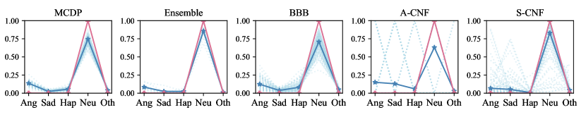
(a) “MSP-PODCAST_0114_0263.wav”

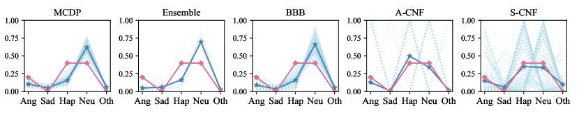
(b) “MSP-PODCAST_0167_0179_0001.wav”

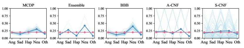
(c) “MSP-PODCAST_0574_0476.wav”

Figure 2: Visualization of simulated annotations on the emotion category annotation task for case study. The y-axis corresponds to the probability mass. Each sample is a categorical distribution. The probability mass values of different categories in each categorical distribution are connected for the purpose of better visualization. CVAE is omitted because it collapses to one category for all inputs.

5.1 Emotion Category Annotation

Task. Emotion recognition aims to identify human emotion, which is beneficial for healthcare, education and customization purposes. Human emotion is inherently ambiguous and the perception of emotion is highly subjective, which often results in disagreements among human annotators. Most emotion recognition datasets employ multiple annotators to label each utterance. However, prior work typically uses the majority vote as the ground-truth target (Busso et al., 2008; Lotfian & Busso, 2019; Poria et al., 2019), which ignores minority viewpoints and thus fails to represent the true human annotation distributions. Our proposed method can enhance the fairness of emotion category annotation as it better handles different opinions among human annotators.

Dataset. MSP-Podcast (Lotfian & Busso, 2019) is one of the largest publicly available datasets in speech emotion recognition, which contains natural English speech from podcast recordings annotated using crowd-sourcing. The experiment uses Release 1.6 of this dataset, which contains more than 50,000 utterances from more than 1,000 speakers consisting of more than 80 hours of speech. The standard splits of training (34,280 segments), validation (5,958 segments) and test (10,124 segments) are used. Emotion labels are grouped into five categories: angry, sad, happy, neutral, and other. Each utterance is labelled by at least 5 human annotators, and there are 6.7 annotations per utterance on average. It is worth noting that 16.5% of the utterances in this dataset do not have a majority emotion class, showing strong disagreement among human annotators.

Performance. Table 1 reports the test results for all compared methods. Ensemble achieves the best majority prediction accuracy (Acc) at the cost of training 10 independent systems. The proposed S-CNF achieves the second-best majority prediction accuracy with only a tenth of the computational cost of Ensemble during training. More importantly, S-CNF is the best at matching the distributions of human annotations (in terms of $\text{NLL}^{\text{all}}$) and simulating inter-annotator disagreements (measured by $\text{RMSE}^{s}$, $\mathcal{E}(\bar{s})$ and $\mathcal{E}(\hat{\kappa})$) among all compared methods.

Case study. To better illustrate the properties of the annotations simulated by different methods, The simulated distributions against the ground-truth distributions for three representative examples are visualized in Figure 2 (more case study examples can be found in Appendix H). Overall, the mean of the samples generated by S-CNF aligns the best with the average human label, indicating its superior performance in estimating the aggregated behaviours of human annotators. Interestingly, the samples generated by S-CNF are the most diverse among all compared methods, which manage to simulate the variability of the behaviours of different individual human annotators. In sharp contrast, the samples generated by all the other methods highly concentrate around their sample means. The visualized result for each example is analyzed below:

1. Human annotators reach a consensus in this case. The majority of samples generated by S-CNF exhibit prominent peaks aligned with the ground-truth emotion class “neutral”. In contrast, many samples generated by A-CNF peak at other emotion classes.

2. Human opinions diverge in this case. The majority of samples generated by S-CNF are sharp categorical distributions peaking at one of the two majority emotion classes “happy” and “neutral”. Additionally, a few samples generated by S-CNF peak at the emotion class “angry”, which manages to simulate the minority viewpoint held by some annotators. Very few human annotators attribute this utterance to the emotion classes “sad” and “other”, and S-CNF likewise produces scarce samples peaking at these classes.

3. Five human annotators give distinct emotion labels in this case, resulting in a tie in the label means. The tie comes from annotators’ diverse individual perceptions of the emotion rather than consensus on its ambiguity. S-CNF is the only model that can simulate both the diverse behaviours of different individual annotators and the aggregated behaviour of all annotators since the individual samples are sharp categorical distributions peaking at one of the five emotion classes and the mean of the samples aligns well with the label mean.

5.2 Toxic Speech Detection

Task. Toxic speech detection aims to filter out harmful and offensive language in written or spoken communications, such as insults, threats and harassment, which can lead to emotional distress, cyberbullying, and hostile online environments. Developing effective toxic detection methods is crucial for creating safer and more respectful online environments and promoting positive interactions and healthy communications among users. Our proposed method incorporates interpretations from different human annotators, leading to a comprehensive understanding of hate speech, which is a good substitute for human annotators to reduce their exposure to distressing and harmful content.

Dataset. The HateXplain dataset (Mathew et al., 2021) is used in this experiment, which contains over 20,000 text posts from Twitter and Gab. These posts are labelled using crowd-sourcing with the commonly used 3-category annotation: hate, offensive, normal. Each post is annotated by three annotators. Cases where all the three annotators choose a different class (919 out of 20,148 posts) were originally excluded from the standard split of the dataset. We incorporate these cases into our training, validation, and test sets in an 8:1:1 ratio to better reflect the inter-annotator disagreements, resulting in 16,118 posts for training, 2,014 for validation, and 2,016 for testing in total.

Performance. Table 2 reports the test results for all compared methods, which shows a similar trend to that found in emotion category annotation experiment in Section 5.1. The Ensemble achieves the best majority prediction accuracy at the cost of training 10 independent systems. Our proposed S-CNF achieves the second best majority prediction accuracy while being much more computationally efficient and has the best performance in distribution matching and inter-annotator disagreement simulation. A case study with visualization can be found in Appendix I, which also exhibits similar trends to those for the emotion category annotation experiment in Section 5.1.

Table 2: Test performance on the toxic speech detection task. CVAE collapses to one category for all inputs.

	Acc$~{}(\uparrow)$	$\text{NLL}^{\text{all}}~{}(\downarrow)$	$\text{RMSE}^{s}~{}(\downarrow)$	$\mathcal{E}(\bar{s})~{}(\downarrow)$	$\mathcal{E}(\hat{\kappa})~{}(\downarrow)$
MCDP	0.656$\pm$0.009	0.951$\pm$0.032	0.300$\pm$0.002	0.129$\pm$0.003	0.143$\pm$0.008
Ensemble	0.682$\pm$0.002	0.909$\pm$0.012	0.289$\pm$0.001	0.100$\pm$0.003	0.064$\pm$0.006
BBB	0.670$\pm$0.001	0.949$\pm$0.021	0.300$\pm$0.009	0.127$\pm$0.022	0.207$\pm$0.051
DPN	0.581$\pm$0.006	1.158$\pm$0.002	0.296$\pm$0.001	0.193$\pm$0.001	0.104$\pm$0.016
CVAE	0.406$\pm$0.000	1.150$\pm$0.000	0.345$\pm$0.000	0.208$\pm$0.000	—
A-CNF	0.628$\pm$0.003	0.892$\pm$0.011	0.297$\pm$0.001	0.087$\pm$0.008	0.198$\pm$0.027
S-CNF	0.673$\pm$0.002	0.837$\pm$0.008	0.263$\pm$0.001	0.002$\pm$0.001	0.026$\pm$0.012

5.3 Speech Quality Assessment

Task. Speech quality assessment plays an important role in the development of speech processing systems such as text-to-speech (TTS) synthesis. Speech quality is a complex, subjective psychoacoustic outcome of human perception. The mean opinion score (MOS) is a commonly used metric to evaluate the speech quality in TTS, which is obtained by having human listeners rate the perceived quality of the synthesized speech on a numerical scale typically ranging from 1 to 5, where a higher score indicates better-perceived speech quality, then averaging the scores across all listeners. However, estimating only the MOS (i.e., the average score) and ignoring the individual scores fails to take into account the subjective nature of individual preferences, perceptions and biases. Our proposed method is a cost-effective alternative to the time-consuming and expensive human assessment of speech quality which models the subjectivity that different human listeners may have.

Dataset. The SOMOS dataset (Maniati et al., 2022) is used in this experiment, which consists of 20,000 synthetic utterances generated from 200 TTS systems and is annotated using crowd-sourcing. Each audio segment is evaluated by at least 17 unique annotators out of 987 participated human annotators, and there are 17.9 annotations per segment on average. The human annotators were asked to evaluate the naturalness of each audio sample on a 5-point Likert scale from 1 (very unnatural) to 5 (completely natural). The standard split provided by the dataset is used, which contains 141,100 training segments, 3,000 validation segments and 3,000 test segments.

Performance. Table 3 reports the test results for all compared methods. Again, our proposed I-CNF obtains the best performance for distribution match and inter-annotator disagreement simulation while achieving the second-best performance for MOS prediction.

Table 3: Test performance on the speech quality assessment task.

	$\text{RMSE}^{\bar{y}}~{}(\downarrow)$	$\text{NLL}^{\text{all}}~{}(\downarrow)$	$\text{RMSE}^{s}~{}(\downarrow)$	$\mathcal{E}(\bar{s})~{}(\downarrow)$
GP	0.359$\pm$0.001	1.693$\pm$0.000	0.472$\pm$0.000	0.412$\pm$0.000
EDL	0.449$\pm$0.023	1.636$\pm$0.001	0.375$\pm$0.022	0.356$\pm$0.025
MCDP	0.390$\pm$0.013	1.787$\pm$0.008	0.783$\pm$0.035	0.742$\pm$0.031
Ensemble	0.410$\pm$0.008	1.858$\pm$0.000	0.740$\pm$0.007	0.704$\pm$0.006
BBB	0.613$\pm$0.011	1.934$\pm$0.015	0.944$\pm$0.017	0.918$\pm$0.017
CVAE	0.419$\pm$0.013	1.703$\pm$0.022	0.598$\pm$0.033	0.561$\pm$0.035
I-CNF	0.392$\pm$0.016	1.609$\pm$0.003	0.251$\pm$0.007	0.123$\pm$0.013

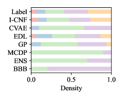
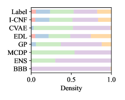
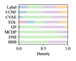
(a) “booksent_2013_0010_051”

(b) “news_2010_0183_165”

(c) “reportorial_2011_0245_098”

Figure 3: Visualization of simulated annotations on the speech quality assessment task for case study. The length of the bar in each colour represents the density of the corresponding score.

Case study. To better illustrate the properties of the annotations simulated by different methods, simulated distributions are visualized against the ground-truth distributions for three representative examples in Figure 3. It can be seen that the proposed I-CNF is the only method which gives an accurate distribution match and perfect inter-annotator disagreement simulation in all three cases. In contrast, all the other methods tend to either produce annotations centered around the mean score or collapse to one score (typically 3 or 4). More case study examples can be found in Appendix J.

6 Conclusion

This paper studied human annotator simulation (HAS), a cost-effective alternative to generating human-like annotation for automatic data labelling and model evaluation. To incorporate the variability of human evaluations, a novel framework was introduced which treats HAS as a zero-shot density estimation problem. This overcame the drawbacks of prior work and enabled efficient annotation simulation for unlabelled test inputs. Under this framework, a meta-learning objective was derived for two new model classes, conditional integer flows and conditional softmax flows, to account for ordinal and categorical annotations, respectively. The proposed method consistently and significantly outperformed a wide range of methods on three real-world human evaluation tasks, achieving the best performance for human annotation distribution matching and inter-annotator disagreement simulation. It is hoped that our proposed method could help mitigate unfair biases and over-representation in HAS and reduce the exposure of human annotators to potentially harmful content, thus promoting ethical AI practices.

Ethics Statement

In this work, all human annotations used for training were taken from existing publicly available corpora, and no new human annotations were collected.

It is hoped that this work could play a part in promoting ethical AI practice. Firstly, it has been shown that the proposed HAS system can capture the inherent variability in human judgements and help mitigate biases and the issue of over-representation, thus producing a more inclusive representation of human opinions. The proposed HAS system also has the potential to minimize human annotators’ exposure to offensive and/or hateful content in some evaluation tasks such as HateXplain.

Reproducibility Statement

The datasets used in the experiments are all publicly available. The source code associated with the proposed method can be found at https://github.com/W-Wu/HAS_CNF.

Appendices

Appendix A The Sources of Variability in Human Evaluation

Human perception refers to the process by which individuals interpret and make sense of the sensory information they receive from the environment. It involves the integration of sensory data, cognitive processes, emotions, and previous experiences. Subjective perception emphasizes that each individual’s perception of the world is unique and influenced by their internal mental states, beliefs, attitudes, and past experiences. As a result, people can interpret and react to the same stimuli differently, leading to diverse and subjective perceptions.

Each person’s sensory organs, such as eyes and ears, may have slight variations in sensitivity and acuity, leading to different perceptions of the same stimuli. Cognitive biases, the inherent mental shortcuts or tendencies that influence how humans perceive and process information, can lead to difference in judgement and decision-making. People’s past experiences, cultural norms, and upbringing also shape their perceptions. Different cultural backgrounds can lead to distinct interpretations of the same event, leading to diverse reaction. The variability in humans can manifest in various tasks such as colour perception, emotion recognition, art appreciation, and feedback preferences.

Embracing and understanding the variability of human perception is vital for various research fields such as psychology, neuroscience, human-computer interaction, and so on, and has practical implications in designing human-centered systems and promoting empathy and diversity. It helps create products and interfaces that cater to diverse user needs and preferences in fields like human-computer interaction and user experience design. Being aware of the variability of perception is crucial in ethical decision-making. It help ensures that different perspectives and cultural sensitivities are considered, which helps identify and address potential biases that might disproportionately affect certain groups or lead to unfair outcomes.

Appendix B Derivations

Detailed derivations for the training objectives on a single dataset $\mathcal{D}_{i}=\{{\bm{\eta}}_{i}^{(1)},\cdots,{\bm{\eta}}_{i}^{(M)}\}$ with ${\bm{x}}_{i}$ are presented in this section. For the simplicity of notations, the subscription $i$ in our derivations will be omitted without ambiguity where possible. The meta-learning objectives presented in the paper are obtained by averaging such single-task objectives across tasks.

B.1 Objective Function for the Base CNF and I-CNF

Denote the empirical human annotation distribution as ${\textnormal{p}}_{m}({\bm{y}}|{\bm{x}})=\delta\left({\bm{y}}-{\bm{\eta}}^{(m)}\right),\ m=1,\cdots,M$ and model output distribution as ${\textnormal{p}}_{\bm{\theta}}({\bm{y}}|{\bm{x}})$. The average KL divergence between them over all $M$ human annotations for this input ${\bm{x}}$ is given by:

$$\mathcal{L}({\bm{\theta}};\mathcal{D},{\bm{x}}) =\frac{1}{M}\sum_{m=1}^{M}\mathcal{KL}\left({\textnormal{p}}_{m}({\bm{y}}|{\bm{x}})\parallel{\textnormal{p}}_{\bm{\theta}}({\bm{y}}|{\bm{x}})\right)$$ (10)

$$=\frac{1}{M}\sum_{m=1}^{M}\int{\textnormal{p}}_{m}({\bm{y}}|{\bm{x}})\log\frac{{\textnormal{p}}_{m}({\bm{y}}|{\bm{x}})}{{\textnormal{p}}_{\bm{\theta}}({\bm{y}}|{\bm{x}})}d{\bm{y}}$$

$$=-\frac{1}{M}\sum_{m=1}^{M}\int{\textnormal{p}}_{m}({\bm{y}}|{\bm{x}})\log{\textnormal{p}}_{\bm{\theta}}({\bm{y}}|{\bm{x}})d{\bm{y}}+\text{const}$$

$$=-\frac{1}{M}\sum_{m=1}^{M}\log{\textnormal{p}}_{\bm{\theta}}({\bm{\eta}}^{(m)}|{\bm{x}})+\text{const}$$

Minimizing this KL objective is equivalent to maximizing the average log likelihood $\log{\textnormal{p}}_{\bm{\theta}}({\bm{\eta}}^{(m)}|{\bm{x}})$ over all human annotations as presented in the paper. With numerical approximation, the training objective for I-CNF shares the same formula as that for the base CNF.

B.2 Objective Function of S-CNF

For categorical annotations, each label ${\bm{\eta}}^{(m)}$ represents the probabilities of all categories in the categorical human annotation distribution: ${\bm{\eta}}^{(m)}=[{\bm{\eta}}_{1}^{(m)},\cdots,{\bm{\eta}}_{K}^{(m)}]$, where ${\bm{\eta}}_{k}^{(m)}={\textnormal{P}}_{m}(c=k|{\bm{x}})$. Denote the model output distribution as ${\textnormal{P}}_{\bm{\theta}}(c|{\bm{x}})$. The average KL divergence between them over all $M$ human annotations for this input ${\bm{x}}$ is given by:

$$\mathcal{L}^{\text{exact}}({\bm{\theta}};\mathcal{D},{\bm{x}}) =\frac{1}{M}\sum_{m=1}^{M}\mathcal{KL}\left({\textnormal{P}}_{m}(c|{\bm{x}})\parallel{\textnormal{P}}_{\bm{\theta}}(c|{\bm{x}})\right)$$ (11)

$$=\frac{1}{M}\sum_{m=1}^{M}\sum_{k=1}^{K}{\textnormal{P}}_{m}(c=k|{\bm{x}})\log\frac{{\textnormal{P}}_{m}(c=k|{\bm{x}})}{{\textnormal{P}}_{\bm{\theta}}(c=k|{\bm{x}})}$$

$$=-\frac{1}{M}\sum_{m=1}^{M}\sum_{k=1}^{K}{\textnormal{P}}_{m}(c=k|{\bm{x}})\log{\textnormal{P}}_{\bm{\theta}}(c=k|{\bm{x}})+\text{const}$$

$$=-\frac{1}{M}\sum_{m=1}^{M}\sum_{k=1}^{K}{\bm{\eta}}_{k}^{(m)}\log{\textnormal{P}}_{\bm{\theta}}(c=k|{\bm{x}})+\text{const},$$

where the marginal likelihood is lower bounded using variational inference:

$$\log{\textnormal{P}}_{\bm{\theta}}(c=k|{\bm{x}}) =\log\int{\textnormal{P}}(c=k|{\bm{v}}){\textnormal{p}}_{\bm{\theta}}({\bm{v}}|{\bm{x}})d{\bm{v}}$$ (12)

$$=\log\int{\bm{q}}_{\bm{\Omega}}({\bm{v}}|{\bm{\eta}})\frac{{\textnormal{P}}(c=k|{\bm{v}}){\textnormal{p}}_{\bm{\theta}}({\bm{v}}|{\bm{x}})}{{\bm{q}}_{\bm{\Omega}}({\bm{v}}|{\bm{\eta}})}d{\bm{v}}$$

$$\geq\int{\bm{q}}_{\bm{\Omega}}({\bm{v}}|{\bm{\eta}})\log\frac{{\textnormal{P}}(c=k|{\bm{v}}){\textnormal{p}}_{\bm{\theta}}({\bm{v}}|{\bm{x}})}{{\bm{q}}_{\bm{\Omega}}({\bm{v}}|{\bm{\eta}})}d{\bm{v}}$$

$$=\mathds{E}_{{\bm{q}}_{\bm{\Omega}}({\bm{v}}|{\bm{\eta}})}\left[\log{\textnormal{P}}(c=k|{\bm{v}})+\log{\textnormal{p}}_{\bm{\theta}}({\bm{v}}|{\bm{x}})-\log{\bm{q}}_{\bm{\Omega}}({\bm{v}}|{\bm{\eta}})\right].$$

Therefore, the final negative ELBO objective is obtained by

$$\mathcal{L}^{\text{exact}} =-\frac{1}{M}\sum_{m=1}^{M}\sum_{k=1}^{K}{\bm{\eta}}_{k}^{(m)}\log{\textnormal{P}}_{\bm{\theta}}(c=k|{\bm{x}})$$ (13)

$$\leq-\frac{1}{M}\sum_{m=1}^{M}\sum_{k=1}^{K}{\bm{\eta}}_{k}^{(m)}\mathds{E}_{{\bm{q}}_{\bm{\Omega}}({\bm{v}}|{\bm{\eta}}^{(m)})}\left[\log{\textnormal{P}}(c=k|{\bm{v}})+\log{\textnormal{p}}_{\bm{\theta}}({\bm{v}}|{\bm{x}})-\log{\bm{q}}_{\bm{\Omega}}({\bm{v}}|{\bm{\eta}}^{(m)})\right]$$

$$=-\frac{1}{M}\sum_{m=1}^{M}\mathds{E}_{{\bm{q}}_{\bm{\Omega}}({\bm{v}}|{\bm{\eta}}^{(m)})}\left[\sum_{k=1}^{K}{\bm{\eta}}_{k}^{(m)}\log{\textnormal{P}}(c=k|{\bm{v}})+\log{\textnormal{p}}_{\bm{\theta}}({\bm{v}}|{\bm{x}})-\log{\bm{q}}_{\bm{\Omega}}({\bm{v}}|{\bm{\eta}}^{(m)})\right]$$

$$=\mathcal{L}({\bm{\theta}},{\bm{\Lambda}};\mathcal{D},{\bm{x}}),$$

where

$$\log{\textnormal{P}}(c=k|{\bm{v}})=\operatorname{logsoftmax}({\bm{v}})_{k},$$ (14)

$$\log{\textnormal{p}}_{\bm{\theta}}({\bm{v}}|{\bm{x}})={\textnormal{p}}_{\bm{\Lambda}}\left({\bm{f}}^{-1}_{\bm{\theta}}({\bm{v}})|{\bm{x}}\right)\left|\operatorname{det}\left(\frac{\partial{\bm{f}}^{-1}_{\bm{\theta}}({\bm{v}})}{\partial{\bm{v}}}\right)\right|,$$ (15)

$$\log{\bm{q}}_{\bm{\Omega}}({\bm{v}}|{\bm{\eta}}^{(m)})=\mathcal{N}({\bm{v}}|{\bm{\mu}}_{\bm{\Omega}}({\bm{\eta}}^{(m)}),{\operatorname{diag}}({\bm{\sigma}}_{\bm{\Omega}}^{2}({\bm{\eta}}^{(m)}))).$$ (16)

B.3 The Negative Log Likelihood ($\text{NLL}^{\text{all}}_{i}$) for Categorical Annotations

The marginal likelihood of S-CNF is intractable, which can be approximated using Monte-Carlo simulation:

$${\textnormal{P}}_{\bm{\theta}}(c=k|{\bm{x}}) =\int{\textnormal{P}}(c=k|{\bm{v}}){\textnormal{p}}_{\bm{\theta}}({\bm{v}}|{\bm{x}})d{\bm{v}}$$ (17)

$$=\mathds{E}_{{\textnormal{p}}_{\bm{\theta}}({\bm{v}}|{\bm{x}})}\left[{\textnormal{P}}(c=k|{\bm{v}})\right]$$

$$\approx\frac{1}{Q}\sum_{j=1}^{Q}{\textnormal{P}}(c=k|{\bm{v}}_{j}),\quad\{{\bm{v}}_{j}\}_{j=1}^{Q}\sim_{\text{iid}}{\textnormal{p}}_{\bm{\theta}}({\bm{v}}|{\bm{x}})$$

$$=\frac{1}{Q}\sum_{j=1}^{Q}\mathrm{softmax}({\bm{v}}_{j})_{k},\quad\{{\bm{v}}_{j}\}_{j=1}^{Q}\sim_{\text{iid}}{\textnormal{p}}_{\bm{\theta}}({\bm{v}}|{\bm{x}})$$

$$=\bar{{\bm{y}}}_{k},$$

where $\bar{{\bm{y}}}=\frac{1}{Q}\sum_{j=1}^{Q}\mathrm{softmax}({\bm{v}}_{j})=\frac{1}{Q}\sum_{j=1}^{Q}{\bm{y}}_{j}$ which is the average of the simulated categorical distributions. Let $\bar{{\bm{\eta}}}=\frac{1}{M}\sum_{m=1}^{M}{\bm{\eta}}^{(m)}$ be the average label.

Then, the $\text{NLL}_{i}^{\text{all}}$ for a single input ${\bm{x}}_{i}$ is given by

$$\text{NLL}^{\text{all}}_{i} =-\frac{1}{M}\sum_{m=1}^{M}\sum_{k=1}^{K}{\bm{\eta}}_{i,k}^{(m)}\log{\textnormal{P}}_{\bm{\theta}}(c=k|{\bm{x}}_{i})$$ (18)

$$\approx-\frac{1}{M}\sum_{m=1}^{M}\sum_{k=1}^{K}{\bm{\eta}}_{i,k}^{(m)}\log\bar{{\bm{y}}}_{i,k}$$

$$=-\sum_{k=1}^{K}\bar{{\bm{\eta}}}_{i,k}\log\bar{{\bm{y}}}_{i,k},$$

which is the cross entropy between the averaged label and averaged sample.

Appendix C Emotion Label Processing for MSP-Podcast

In MSP-Podcast, each annotator can choose from ten emotion classes to label the primary emotion of an utterance: Angry, Sad, Happy, Surprise, Fear, Disgust, Contempt, Neutral, Other. Although only one option is allowed, they can say other and define their own emotion class which can be more than one. During label processing, the original other class is split into sub-classes depending on the manual defined label and merged with the pre-defined labels. The grouping details are shown as follows: (i) Angry includes angry, disgust, contempt, annoyed; (ii) Sad includes sad, frustrated, disappointed, depressed, concerned; (iii) Happy includes happy, excited, amused; (iv) Neutral includes neutral; (v) Other includes all other emotion subclasses not listed above.

Appendix D Model Structure Details

The structure of proposed I-CNF and S-CNF are illustrated in Figure 4 and Figure 5 respectively. The procedure of sampling from and optimizing S-CNF are summarized in Algorithm 1 and 2.

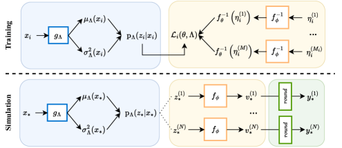
Figure 4: Illustration for I-CNF training and simulation workflow.

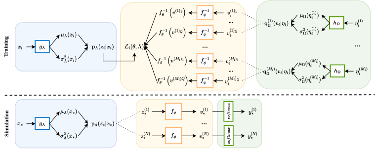
Figure 5: Illustration for S-CNF training and simulation workflow.

Algorithm 1 Sampling from S-CNF

Input: ${\bm{x}}$

Output: Categorical probability ${\bm{y}}$

Compute ${\bm{\mu}}_{\bm{\Lambda}}({\bm{x}}),{\bm{\sigma}}_{\bm{\Lambda}}^{2}({\bm{x}})={\bm{g}}_{\bm{\Lambda}}({\bm{x}})$

Sample ${\bm{z}}\sim\mathcal{N}({\bm{\mu}}_{\bm{\Lambda}}({\bm{x}}),{\operatorname{diag}}({\bm{\sigma}}_{\bm{\Lambda}}^{2}({\bm{x}}))$

Compute ${\bm{v}}={\bm{f}}_{\bm{\theta}}\left({\bm{z}}\right)$

Compute ${\bm{y}}=\mathrm{softmax}({\bm{v}})$

Algorithm 2 Optimizing S-CNF

Input: ${\bm{x}},\mathcal{D}=\{{\bm{\eta}}^{(1)},\cdots,{\bm{\eta}}^{(M)}\}$

Output: ELBO $\mathcal{L}^{\text{ELBO}}$ on dataset $\mathcal{D}$

for $m=1,\cdots,M$ do

     Compute ${\bm{\mu}}_{\bm{\Omega}}({\bm{\eta}}^{(m)}),{\bm{\sigma}}_{\bm{\Omega}}^{2}({\bm{\eta}}^{(m)})={\bm{h}}_{\bm{\Omega}}({\bm{\eta}}^{(m)})$

     for $j=1,\cdots,Q$ do

         Sample ${\bm{v}}_{j}\sim{\bm{q}}_{\bm{\Omega}}({\bm{v}}|{\bm{\eta}}^{(m)})$

         Compute $\mathcal{L}_{j}^{(m)}=-\sum_{k=1}^{K}{\bm{\eta}}_{k}^{(m)}\log{\textnormal{P}}(c=k|{\bm{v}}_{j})+\log{\textnormal{p}}_{\bm{\theta}}({\bm{v}}_{j}|{\bm{x}})-\log{\bm{q}}_{\bm{\Omega}}({\bm{v}}_{j}|{\bm{\eta}}^{(m)})$

     end for

     Compute $\mathcal{L}_{m}^{\text{ELBO}}=\frac{1}{Q}\sum_{j=1}^{Q}\mathcal{L}_{j}^{(m)}$

end for

Compute $\mathcal{L}^{\text{ELBO}}=\frac{1}{M}\sum_{m=1}^{M}\mathcal{L}_{m}^{\text{ELBO}}$

A neural-network-based encoder ${\bm{g}}_{\bm{\Lambda}}$ is built to model ${\bm{\mu}}_{\bm{\Lambda}}({\bm{x}}),{\bm{\sigma}}_{\bm{\Lambda}}^{2}({\bm{x}})$ given input ${\bm{x}}$ where ${\bm{\Lambda}}$ is the model parameters. ${\bm{g}}_{\bm{\Lambda}}$ follows an upstream-downstream paradigm. The upstream model is pretrained on large amount of unlabelled data to learn universal representations. The downstream model uses the learned representation from the upstream model for specific applications. In this paper, the downstream model consists of two Transformer encoder blocks followed by two FC layers. The output layer contains two heads to predict the mean and standard deviation of the latent distribution ${\textnormal{p}}_{\bm{\Lambda}}({\bm{z}}|{\bm{x}})$.

For tasks involving speech as input (i.e., emotion class labelling, speech quality prediction), WavLM (Chen et al., 2022) is used as the upstream model. WavLM is a speech foundation model pre-trained by self-supervised learning that takes raw waveform as input. The waveform is encoded by a CNN encoder followed by multiple Transformer encoders. The BASE+ version of the model is used in this work which has 12 Transformer encoder blocks with 768-dimensional hidden states and 8 attention heads. The parameters of the pretrained WavLM are frozen and the weighted sum of the outputs of the 12 Transformer encoder blocks is used as the speech embeddings feeding into the downstream model.

RoBERTa (Liu et al., 2019) is used as upstream model to encode text input for toxic speech detection, which is a robustly optimized model of BERT (Devlin et al., 2019). RoBERTa is a Transformer-based language model pretrained on a large corpus of English data with the masked language modelling objective. The BASE version was used in the work which has 12 Transformer layers, 768 hidden units, 12 attention heads, and 125 million parameters.

The downstream model consists of two Transformer encoder layers with hidden dimension of 128 and four attention head. The invertible flow model ${\bm{f}}_{\bm{\theta}}$ uses real NVP block Dinh et al. (2017). The variational encoder for S-CNF ${\bm{h}}_{\bm{\Omega}}$ contains a FC layer and two output heads for the mean and standard deviation of the variational distribution ${\bm{q}}_{\bm{\Omega}}({\bm{v}}|{\bm{y}})$. More details can be found in Table 4.

Table 4: Dimension of the model structure (number of layers * layer dimension)

Task	input modality	${\bm{g}}_{\bm{\Lambda}}$-upstream	${\bm{g}}_{\bm{\Lambda}}$-downstream	${\bm{f}}_{\bm{\theta}}$	${\bm{h}}_{\bm{\Omega}}$
Emotion class labelling	speech	WavLM base+	2*128	3*64	1*64
Toxic speech detection	text	RoBERTa base	2*128	3*64	1*64
Speech quality assessment	speech	WavLM base+	2*128	3*16	/

Appendix E Detailed Configuration of All Compared Methods

Ensemble consists of 10 systems initialized and trained using different random seeds. MCDP uses dropout rate of 0.4. A standard Gaussian prior is used for BBB. A modified version of EDL is used (Wu et al., 2023) which is trained by maximising the per-observation-based marginal likelihood with a modified regularization term. Ensemble, MCDP, BBB, EDL use the same model structure as ${\bm{g}}_{\bm{\Lambda}}$ apart from removing the output head for predicting variance of latent distribution. A modified version of DPN(Wu et al., 2022b) is used which is trained by interpolating per-observation-based marginal likelihood with KL divergence. The coefficient of KL term is set to 5.0 for emotion class labelling and 2.0 for toxic speech detection. Features extracted from the upstream model are used as input to GP which uses a radial basis function kernel and is trained by maximising the per-observation-based marginal likelihood. CVAE has the same ${\bm{g}}_{\bm{\Lambda}}$ structure as S-CNF for modelling ${\textnormal{p}}({\bm{z}}|{\bm{x}})$, and two 64-d FC layers are used for encoder and decoder. A-CNF has identical model structure as S-CNF.

The system was implemented using PyTorch with the SpeechBrain (Ravanelli et al., 2021) and normflows (Stimper et al., 2023) toolkit. The Adadelta optimizer was used with an initial learning rate of 1.2 for emotion class labelling and 0.05 for speech quality assessment. The The NewBob learning rate scheduler was used with annealing factor 0.8 and patience 1. The system was trained for 30 epochs and the model with the best validation performance was used for testing. The number of ELBO samples was set to 20.

Appendix F Analysis of Standard Deviation of Simulated Samples

It has been observed in Section 5.1 that flow models tend to have a larger difference between $\text{RMSE}^{s}$ and $\mathcal{E}(\bar{s})$. This section provides detailed analysis to this observation. Let $N$ be the number of test utterances. Three std-related metrics are computed: (i) RMSE between std of predictions and human labels: $\text{RMSE}^{s}=\sqrt{\frac{1}{N}\sum_{i=1}^{N}\left(s_{i}-\sigma_{i}\right)^{2}}$; (ii) Mean absolute error between std of predictions and std of human labels: $\text{MAE}^{s}=\frac{1}{N}\sum_{i=1}^{N}|s_{i}-\sigma_{i}|$; (iii) Absolute error between average std of predictions and average std of human labels $\mathcal{E}(\bar{s})=\left|\bar{s}_{i}-\bar{\sigma}_{i}\right|$. Results are shown in Table 5.

Table 5: Analysis of standard deviation of simulated samples

	Emotion recognition			Toxic detection			Speech quality
	$\text{RMSE}^{s}$	$\text{MAE}^{s}$	$\mathcal{E}(\bar{s})$	$\text{RMSE}^{s}$	$\text{MAE}^{s}$	$\mathcal{E}(\bar{s})$	$\text{RMSE}^{s}$	$\text{MAE}^{s}$	$\mathcal{E}(\bar{s})$
MCDP	0.305	0.233	0.206	0.297	0.242	0.122	0.809	0.762	0.762
Ensemble	0.277	0.222	0.166	0.290	0.220	0.105	0.747	0.703	0.703
BBB	0.284	0.226	0.178	0.279	0.229	0.115	0.952	0.917	0.917
CVAE	0.333	0.244	0.244	0.345	0.208	0.208	0.574	0.535	0.534
EDL	/			/			0.381	0.368	0.368
GP	/			/			0.472	0.419	0.412
DPN	0.297	0.236	0.191	0.299	0.220	0.178	/
A-CNF	0.223	0.209	0.046	0.274	0.232	0.062	/
S/I-CNF	0.218	0.198	0.015	0.263	0.206	0.002	0.229	0.184	0.067

The flow model tends to have larger discrepancy between $\text{MAE}^{s}$ and $\mathcal{E}(\bar{s})$. According to the triangular inequality:

$$\mathcal{E}(\bar{s})=\left|\frac{1}{N}\sum_{i=1}^{N}s_{i}-\frac{1}{N}\sum_{i=1}^{N}\sigma_{i}\right|=\left|\frac{1}{N}\sum_{i=1}^{N}(s_{i}-\sigma_{i})\right|\leq\frac{1}{N}\sum_{i=1}^{N}\left|s_{i}-\sigma_{i}\right|=\text{MAE}^{s}$$ (19)

which show that $\mathcal{E}(\bar{s})$ is a lower bound of $\text{MAE}^{s}$. The equality condition is satisfied when all samples are uniformly either greater than or less than the compared value. Therefore, a larger discrepancy between these two values indicates that the standard deviation of some samples exceeds that of the labels, while for others, it is lower. A smaller discrepancy indicates that the standard deviation of samples tend to be consistently larger of smaller than that of the labels. In Figure 6, 100 test utterances are randomly selected and the std of samples generated by different models are plotted, which supports the above conclusion. The proposed S-CNF and I-CNF has the best performance for matching the diversity of human annotations.

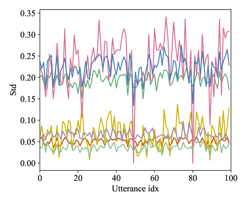
(a) Std for emotion class labelling.

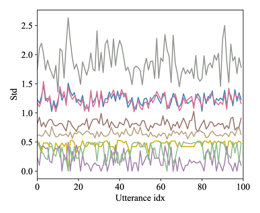
(b) Std for speech quality evaluation.

Figure 6: Standard deviation of simulated samples.

Appendix G Adjusting Diversity of CNFs by Prior Tempering

One advantage of CNF is that its sample diversity can be easily controlled on demand without re-training by tempering the standard deviation of ${\textnormal{p}}_{\bm{\Lambda}}({\bm{z}}|{\bm{x}})$ at test time. Figure LABEL:fig:_T-softmax-appendix explores the effect of prior tempering on the performance. More details are shown in Table 6. Overall, the trend is clear that the simulated annotations become more diverse as the temperature increases. The default temperature value $1$ used during training (i.e., no tempering) achieves the best trade-off among majority prediction accuracy (Acc), distribution matching ($\text{NLL}^{\text{all}}$), and inter-annotator disagreement simulation (in terms of $\mathcal{E}(\bar{s})$ and $\mathcal{E}(\hat{\kappa})$). In addition, as compared in Table 7, prior tempering in CNF is more efficient and covers a wider range of dynamics than adjusting the dropout rate in MCDP.

(a) Emotion class labelling

(b) Toxic speech detection

Table 6: Adjusting the diversity of CNFs by prior tempering.

Emotion class labelling
T	Acc	$\text{NLL}^{\text{all}}$	$\text{RMSE}^{s}$	$\bar{s}$	$\mathcal{E}(\bar{s})$	$\hat{\kappa}$	$\mathcal{E}(\hat{\kappa})$
0.8	0.594	1.395	0.221	0.200	0.044	0.307	0.053
0.9	0.594	1.390	0.219	0.216	0.029	0.259	0.005
1.0	0.593	1.389	0.218	0.229	0.015	0.222	0.032
1.1	0.592	1.389	0.218	0.241	0.004	0.191	0.063
1.2	0.590	1.391	0.219	0.251	0.007	0.166	0.088
Toxic speech detection
T	Acc	$\text{NLL}^{\text{all}}$	$\text{RMSE}^{s}$	$\bar{s}$	$\mathcal{E}(\bar{s})$	$\hat{\kappa}$	$\mathcal{E}(\hat{\kappa})$
0.8	0.671	0.851	0.272	0.125	0.065	0.721	0.115
0.9	0.675	0.842	0.265	0.157	0.033	0.650	0.044
1.0	0.673	0.837	0.263	0.188	0.002	0.580	0.026
1.1	0.671	0.836	0.264	0.216	0.026	0.512	0.094
1.2	0.669	0.837	0.267	0.242	0.052	0.450	0.156
Speech quality assessment
T	$\text{RMSE}^{\bar{y}}$	$\text{NLL}^{\text{all}}$	$\text{RMSE}^{s}$	$\bar{s}$	$\mathcal{E}(\bar{s})$	$\hat{\kappa}$	$\mathcal{E}(\hat{\kappa})$
0.8	0.377	1.671	0.274	0.963	0.179	/	/
0.9	0.380	1.624	0.218	1.083	0.059	/	/
1.0	0.384	1.611	0.223	1.201	0.059	/	/
1.1	0.388	1.619	0.281	1.322	0.180	/	/
1.2	0.393	1.640	0.371	1.440	0.299	/	/

Table 7: Adjusting the diversity of MCDP models by dropout rate

Emotion class labelling
dp	Acc	$\text{NLL}^{\text{all}}$	$\text{RMSE}^{s}$	$\bar{s}$	$\mathcal{E}(\bar{s})$	$\hat{\kappa}$	$\mathcal{E}(\hat{\kappa})$
0.1	0.583	1.463	0.303	0.040	0.205	0.791	0.537
0.2	0.589	1.426	0.303	0.040	0.204	0.773	0.519
0.3	0.590	1.415	0.300	0.045	0.199	0.761	0.507
0.4	0.585	1.405	0.296	0.051	0.194	0.723	0.469
0.5	0.589	1.409	0.294	0.053	0.191	0.715	0.461
Toxic speech detection
dp	Acc	$\text{NLL}^{\text{all}}$	$\text{RMSE}^{s}$	$\bar{s}$	$\mathcal{E}(\bar{s})$	$\hat{\kappa}$	$\mathcal{E}(\hat{\kappa})$
0.1	0.661	0.925	0.314	0.049	0.158	0.831	0.225
0.2	0.666	0.916	0.308	0.061	0.147	0.800	0.194
0.3	0.654	0.968	0.299	0.081	0.127	0.750	0.144
0.4	0.662	0.943	0.297	0.085	0.122	0.731	0.125
0.5	0.662	0.896	0.296	0.088	0.120	0.720	0.114
Speech quality assessment
dp	$\text{RMSE}^{\bar{y}}$	$\text{NLL}^{\text{all}}$	$\text{RMSE}^{s}$	$\bar{s}$	$\mathcal{E}(\bar{s})$	$\hat{\kappa}$	$\mathcal{E}(\hat{\kappa})$
0.1	0.385	1.828	0.982	0.180	0.961	/	/
0.2	0.412	1.824	0.928	0.236	0.905	/	/
0.3	0.408	1.797	0.871	0.294	0.847	/	/
0.4	0.367	1.805	0.938	0.227	0.915	/	/
0.5	0.356	1.780	0.889	0.278	0.864	/	/

Appendix H Additional Visualization for Emotion Class Labelling

This section shows additional visualized examples for emotion class labelling when human annotators reach a consensus (Figure 8 (a)(b)), diverge (Figure 8 (c)(d)), and give distinct labels (Figure 8 (e)). The proposed S-CNF can better simulate the aggregated behaviour as well as the variability of human annotations in all cases.

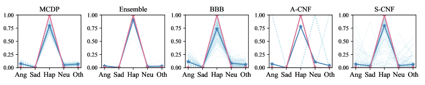
(a) “MSP-PODCAST_1216_0067.wav”

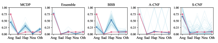
(b) “MSP-PODCAST_0566_0220”

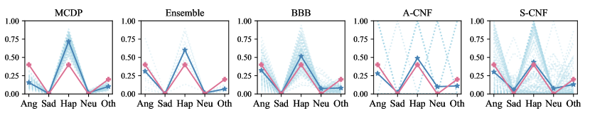
(c) “MSP-PODCAST_0584_0145.wav”

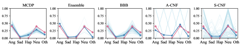
(d) “MSP-PODCAST_0876_0069.wav”

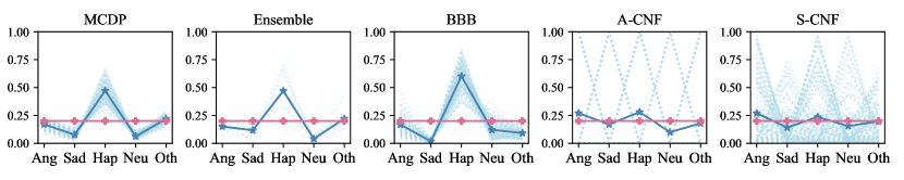
(e) “MSP-PODCAST_0587_0073.wav”

Figure 8: Additional visualized examples for emotion class labelling. The y-axis corresponds to the probability mass. Each sample is a categorical distribution. The probability mass values of different categories in each categorical distribution are connected for the purpose of better visualization. CVAE is omitted because it collapses to one category for all inputs.

Appendix I Additional Visualization for Toxic Speech Detection

This section shows visualized examples for toxic speech detection when all three human annotators provide the same label (Figure 9 (a)(b)), one of them gives a different label (Figure 9 (c)(d)), and all three annoators give distinct labels (Figure 9 (e)). The proposed S-CNF can better simulate the aggregated behaviour as well as the variability of human annotations in all cases.

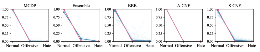
(a) “1092591391086178304_twitter”

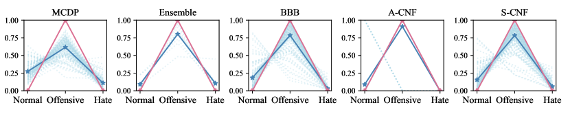
(b) “10665227_gab”

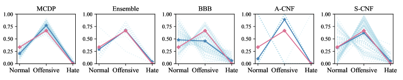
(c) “1179093526098743296_twitter”

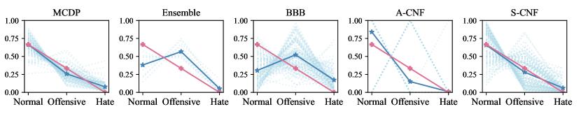
(d) “18777413_gab”

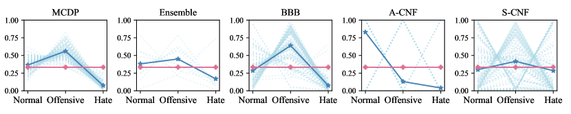
(e) “20362058_gab”

Figure 9: Additional visualized examples for toxic speech detection. The y-axis corresponds to the probability mass. Each sample is a categorical distribution. The probability mass values of different categories in each categorical distribution are connected for the purpose of better visualization. CVAE is omitted because it collapses to one category for all inputs.

Appendix J Additional Visualization for Speech Quality Evaluation

This section presents several additional visualized cases for speech quality evaluation. Generated samples (before rounding) are plotted in the sub-figures on the left. For clearer visualization, the samples are spread along $y$ axis according to density to avoid overlapping. As can be seen, samples generated by the proposed I-CNF method (in blue) can better simulate the diversity of human annotations (in pink).

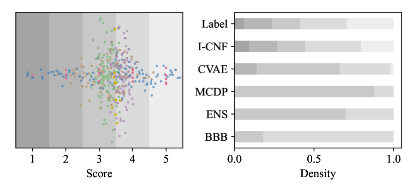
(a) “conv_2007_0090_057”

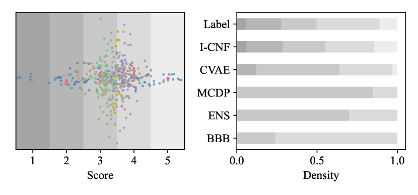
(b) “conv_2007_0090_060”

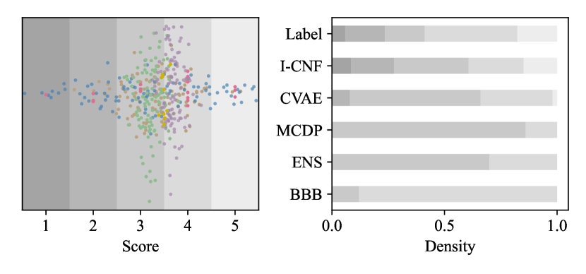
(c) “reportorial_2011_0154_145”

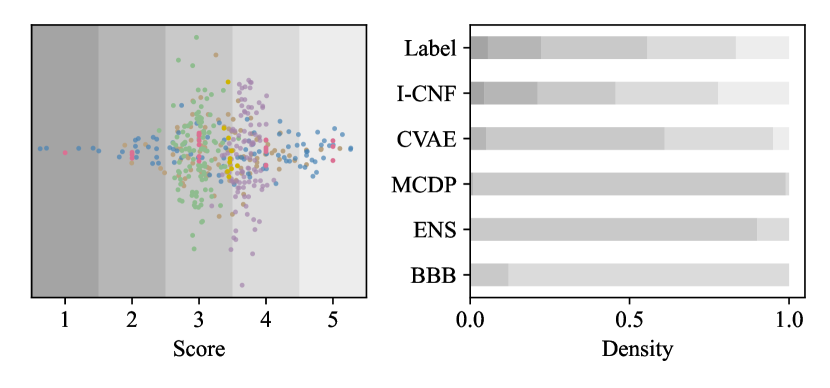
(d) “reportorial_2011_0096_186”

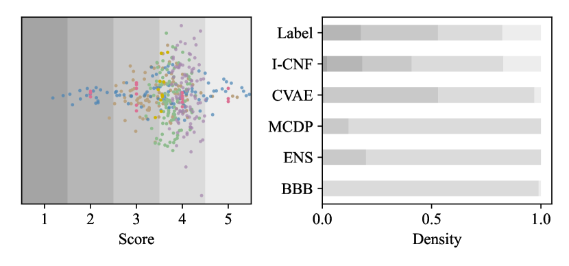
(e) “novel_2011_0011_110”

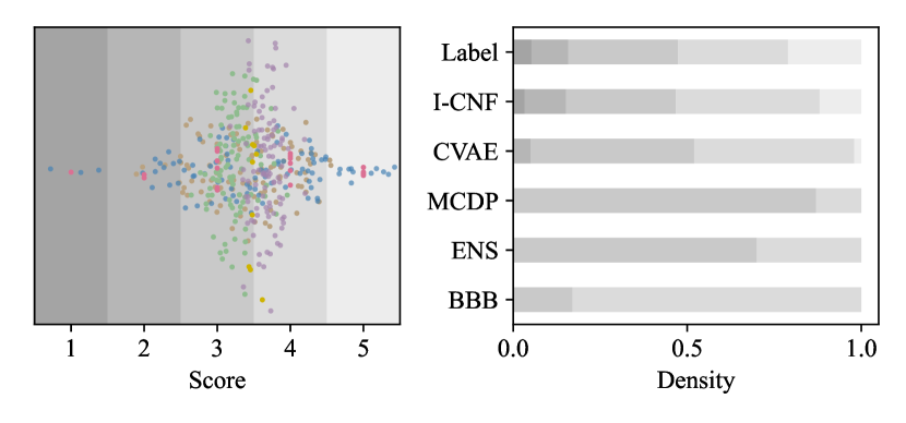
(f) “wiki_0033_055”

Figure 10: Additional visualized examples for speech quality assessment. For the visualization purpose, the points that have same x values are spread along y axis according to density to avoid overlapping.

References

- Alm (2011) Cecilia Ovesdotter Alm. Subjective natural language problems: Motivations, applications, characterizations, and implications. In Proc. ACL, Portland, USA, 2011.
- Amini et al. (2020) Alexander Amini, Wilko Schwarting, Ava Soleimany, and Daniela Rus. Deep evidential regression. In Proc. NeurIPS, Online, 2020.
- Asri et al. (2016) Layla El Asri, Jing He, and Kaheer Suleman. A sequence-to-sequence model for user simulation in spoken dialogue systems. In Proc. Interspeech, San Francisco, USA, 2016.
- Blundell et al. (2015) Charles Blundell, Julien Cornebise, Koray Kavukcuoglu, and Daan Wierstra. Weight uncertainty in neural network. In Proc. ICML, Lille, France, 2015.
- Bommasani et al. (2021) Rishi Bommasani, Drew A Hudson, Ehsan Adeli, Russ Altman, Simran Arora, Sydney von Arx, Michael S. Bernstein, Jeannette Bohg, Antoine Bosselut, Emma Brunskill, et al. On the opportunities and risks of foundation models. arXiv preprint arXiv:2108.07258, 2021.
- Borade & Netak (2020) Jyoti G Borade and Laxman D Netak. Automated grading of essays: a review. In Proc. IHCI, Daegu, South Korea, 2020.
- Busso et al. (2008) C. Busso, M. Bulut, C.-C. Lee, A. Kazemzadeh, E.M. Provost, S. Kim, J.N. Chang, S. Lee, and S.S. Narayanan. IEMOCAP: Interactive emotional dyadic motion capture database. Language Resources and Evaluation, 42:335–359, 2008.
- Chen et al. (2022) Sanyuan Chen, Chengyi Wang, Zhengyang Chen, Yu Wu, Shujie Liu, Zhuo Chen, Jinyu Li, Naoyuki Kanda, Takuya Yoshioka, Xiong Xiao, et al. WavLM: Large-scale self-supervised pre-training for full stack speech processing. IEEE Journal of Selected Topics in Signal Processing, 16(6):1505–1518, 2022.
- Chen et al. (2023) Wenlin Chen, Austin Tripp, and José Miguel Hernández-Lobato. Meta-learning adaptive deep kernel gaussian processes for molecular property prediction. In Proc. ICLR, Kigali, Rwanda, 2023.
- Chou & Lee (2019) Huang-Cheng Chou and Chi-Chun Lee. Every rating matters: Joint learning of subjective labels and individual annotators for speech emotion classification. In Proc. ICASSP, Brighton, UK, 2019.
- Christiano et al. (2017) Paul F. Christiano, Jan Leike, Tom Brown, Miljan Martic, Shane Legg, and Dario Amodei. Deep reinforcement learning from human preferences. In Proc. NIPS, Long Beach, USA, 2017.
- Dang et al. (2017) Ting Dang, Vidhyasaharan Sethu, Julien Epps, and Eliathamby Ambikairajah. An investigation of emotion prediction uncertainty using gaussian mixture regression. In Proc. Interspeech, Stockholm, Sweden, 2017.
- Davani et al. (2022) Aida Mostafazadeh Davani, Mark Díaz, and Vinodkumar Prabhakaran. Dealing with disagreements: Looking beyond the majority vote in subjective annotations. Transactions of the Association for Computational Linguistics, 10:92–110, 2022.
- Deng et al. (2012) Jun Deng, Wenjing Han, and Björn Schuller. Confidence measures for speech emotion recognition: A start. In Speech Communication; 10. ITG Symposium, pp. 1–4. VDE, 2012.
- Devlin et al. (2019) Jacob Devlin, Ming-Wei Chang, Kenton Lee, and Kristina Toutanova. BERT: Pre-training of deep bidirectional transformers for language understanding. In Proc. NAACL, Minneapolis, USA, 2019.
- Dinh et al. (2017) Laurent Dinh, Jascha Sohl-Dickstein, and Samy Bengio. Density estimation using real NVP. In Proc. ICLR, Toulon, France, 2017.
- Dixon et al. (2018) Lucas Dixon, John Li, Jeffrey Sorensen, Nithum Thain, and Lucy Vasserman. Measuring and mitigating unintended bias in text classification. In Proc. AAAI, New Orleans, USA, 2018.
- Djuric et al. (2015) Nemanja Djuric, Jing Zhou, Robin Morris, Mihajlo Grbovic, Vladan Radosavljevic, and Narayan Bhamidipati. Hate speech detection with comment embeddings. In Proc. WWW, Florence, Italy, 2015.
- Fayek et al. (2016) H.M. Fayek, M. Lech, and L. Cavedon. Modeling subjectiveness in emotion recognition with deep neural networks: Ensembles vs soft labels. In Proc. IJCNN, Vancouver, Canada, 2016.
- Fleiss (1971) Joseph L Fleiss. Measuring nominal scale agreement among many raters. Psychological Bulletin, 76(5):378, 1971.
- Gal & Ghahramani (2016) Yarin Gal and Zoubin Ghahramani. Dropout as a Bayesian approximation: Representing model uncertainty in deep learning. In Proc. ICML, New York, USA, 2016.
- Gür et al. (2018) Izzeddin Gür, Dilek Hakkani-Tür, Gokhan Tür, and Pararth Shah. User modeling for task oriented dialogues. In Proc. SLT, Athens, Greece, 2018.
- Han et al. (2017) Jing Han, Zixing Zhang, Maximilian Schmitt, Maja Pantic, and Björn Schuller. From hard to soft: Towards more human-like emotion recognition by modelling the perception uncertainty. In Proc. ACM MM, Mountain View, USA, 2017.
- Haselton et al. (2015) Martie G Haselton, Daniel Nettle, and Paul W Andrews. The evolution of cognitive bias. The Handbook of Evolutionary Psychology, pp. 724–746, 2015.
- Hirschberg et al. (2003) Julia Hirschberg, Jackson Liscombe, and Jennifer Venditti. Experiments in emotional speech. In Proc. SSPR, Tokyo, Japan, 2003.
- Hoogeboom et al. (2021) Emiel Hoogeboom, Didrik Nielsen, Priyank Jaini, Patrick Forré, and Max Welling. Argmax flows and multinomial diffusion: Learning categorical distributions. In M. Ranzato, A. Beygelzimer, Y. Dauphin, P.S. Liang, and J. Wortman Vaughan (eds.), Proc. NeurIPS, Online, 2021.
- Hutchinson et al. (2020) Ben Hutchinson, Vinodkumar Prabhakaran, Emily Denton, Kellie Webster, Yu Zhong, and Stephen Denuyl. Social biases in NLP models as barriers for persons with disabilities. In Proc. ACL, Online, 2020.
- Kim et al. (2013) Y. Kim, H. Lee, and E. M. Provost. Deep learning for robust feature generation in audiovisual emotion recognition. In Proc. ICASSP, Vancouver, Canada, 2013.
- Kingma & Welling (2014) Diederik P Kingma and Max Welling. Auto-encoding variational Bayes. In Proc. ICLR, Banff, Canada, 2014.
- Lakshminarayanan et al. (2017) Balaji Lakshminarayanan, Alexander Pritzel, and Charles Blundell. Simple and scalable predictive uncertainty estimation using deep ensembles. In Proc. NIPS, Long Beach, USA, 2017.
- Leng et al. (2021) Yichong Leng, Xu Tan, Sheng Zhao, Frank Soong, Xiang-Yang Li, and Tao Qin. MBNet: MOS prediction for synthesized speech with mean-bias network. In Proc. ICASSP, Toronto, Canada, 2021.
- Lin et al. (2021) Hsien-Chin Lin, Nurul Lubis, Songbo Hu, Carel van Niekerk, Christian Geishauser, Michael Heck, Shutong Feng, and Milica Gasic. Domain-independent user simulation with transformers for task-oriented dialogue systems. In Proc. SIGDIAL, Singapore City, Singapore, 2021.
- Liu et al. (2019) Yinhan Liu, Myle Ott, Naman Goyal, Jingfei Du, Mandar Joshi, Danqi Chen, Omer Levy, Mike Lewis, Luke Zettlemoyer, and Veselin Stoyanov. RoBERTa: A robustly optimized bert pretraining approach. arXiv preprint arXiv:1907.11692, 2019.
- Lo et al. (2019) Chen-Chou Lo, Szu-Wei Fu, Wen-Chin Huang, Xin Wang, Junichi Yamagishi, Yu Tsao, and Hsin-Min Wang. MOSNet: Deep learning-based objective assessment for voice conversion. In Proc. Interspeech, Graz, Austria, 2019.
- Lotfian & Busso (2019) R. Lotfian and C. Busso. Building naturalistic emotionally balanced speech corpus by retrieving emotional speech from existing podcast recordings. IEEE Transactions on Affective Computing, 10(4):471–483, 2019.
- Ma et al. (2015) Kede Ma, Kai Zeng, and Zhou Wang. Perceptual quality assessment for multi-exposure image fusion. IEEE Transactions on Image Processing, 24(11):3345–3356, 2015.
- Malinin & Gales (2018) Andrey Malinin and Mark Gales. Predictive uncertainty estimation via prior networks. In Proc. NeurIPS, Montreal, Canada, 2018.
- Maniati et al. (2022) Georgia Maniati, Alexandra Vioni, Nikolaos Ellinas, Karolos Nikitaras, Konstantinos Klapsas, June Sig Sung, Gunu Jho, Aimilios Chalamandaris, and Pirros Tsiakoulis. SOMOS: The Samsung open MOS dataset for the evaluation of neural text-to-speech synthesis. In Proc. Interspeech, Incheon, Korea, 2022.
- Mathew et al. (2021) Binny Mathew, Punyajoy Saha, Seid Muhie Yimam, Chris Biemann, Pawan Goyal, and Animesh Mukherjee. HateXplain: A benchmark dataset for explainable hate speech detection. In Proc. AAAI, Vancouver, Canada, 2021.
- Mihalcea & Liu (2006) Rada Mihalcea and Hugo Liu. A corpus-based approach to finding happiness. In Proc. AAAI Spring Symposium, Stanford, USA, 2006.
- Ouyang et al. (2022) Long Ouyang, Jeffrey Wu, Xu Jiang, Diogo Almeida, Carroll Wainwright, Pamela Mishkin, Chong Zhang, Sandhini Agarwal, Katarina Slama, Alex Ray, et al. Training language models to follow instructions with human feedback. In Proc. NeurIPS, New Orleans, USA, 2022.
- Patton et al. (2016) Brian Patton, Yannis Agiomyrgiannakis, Michael Terry, Kevin Wilson, Rif A. Saurous, and D. Sculley. AutoMOS: Learning a non-intrusive assessor of naturalness-of-speech. In Proc, NeurIPS Workshop, Barcelona, Spain, 2016.
- Plank et al. (2014) Barbara Plank, Dirk Hovy, and Anders Søgaard. Learning part-of-speech taggers with inter-annotator agreement loss. In Proc. EACL, Gothenburg, Sweden, 2014.
- Poria et al. (2017) S. Poria, E. Cambria, R. Bajpai, and A. Hussain. A review of affective computing: From unimodal analysis to multimodal fusion. Information Fusion, 37:98–125, 2017.
- Poria et al. (2019) Soujanya Poria, Devamanyu Hazarika, Navonil Majumder, Gautam Naik, Erik Cambria, and Rada Mihalcea. MELD: A multimodal multi-party dataset for emotion recognition in conversations. In Proc. ACL, Florence, Italy, 2019.
- Prabhakaran et al. (2012) Vinodkumar Prabhakaran, Michael Bloodgood, Mona Diab, Bonnie Dorr, Lori Levin, Christine D. Piatko, Owen Rambow, and Benjamin Van Durme. Statistical modality tagging from rule-based annotations and crowdsourcing. In Proc. ExProM Workshop, Jeju, Korea, 2012.
- Rafailov et al. (2023) Rafael Rafailov, Archit Sharma, Eric Mitchell, Stefano Ermon, Christopher D Manning, and Chelsea Finn. Direct preference optimization: Your language model is secretly a reward model. arXiv preprint arXiv:2305.18290, 2023.
- Ramesh & Sanampudi (2022) Dadi Ramesh and Suresh Kumar Sanampudi. An automated essay scoring systems: A systematic literature review. Artificial Intelligence Review, 55(3):2495–2527, 2022.
- Ratner et al. (2016) Alexander J. Ratner, Christopher M De Sa, Sen Wu, Daniel Selsam, and Christopher Ré. Data programming: Creating large training sets, quickly. In Proc. NeurIPS, Barcelona, Spain, 2016.
- Ravanelli et al. (2021) Mirco Ravanelli, Titouan Parcollet, Peter Plantinga, Aku Rouhe, Samuele Cornell, Loren Lugosch, Cem Subakan, Nauman Dawalatabad, Abdelwahab Heba, Jianyuan Zhong, Ju-Chieh Chou, Sung-Lin Yeh, Szu-Wei Fu, Chien-Feng Liao, Elena Rastorgueva, François Grondin, William Aris, Hwidong Na, Yan Gao, Renato De Mori, and Yoshua Bengio. SpeechBrain: A general-purpose speech toolkit. arXiv preprint arXiv:2106.04624, 2021.
- Ruiz et al. (2019) Nataniel Ruiz, Samuel Schulter, and Manmohan Chandraker. Learning to simulate. In Proc. ICLR, New Orleans, USA, 2019.
- Schatzmann et al. (2007) Jost Schatzmann, Blaise Thomson, Karl Weilhammer, Hui Ye, and Steve Young. Agenda-based user simulation for bootstrapping a POMDP dialogue system. In Proc. NAACL, Vancouver, Canada, 2007.
- Seshadrinathan et al. (2010) Kalpana Seshadrinathan, Rajiv Soundararajan, Alan Conrad Bovik, and Lawrence K. Cormack. Study of subjective and objective quality assessment of video. IEEE Transactions on Image Processing, 19(6):1427–1441, 2010.
- Shi et al. (2019) Weiyan Shi, Kun Qian, Xuewei Wang, and Zhou Yu. How to build user simulators to train RL-based dialog systems. In Proc. EMNLP-IJCNLP, Hong Kong, China, 2019.
- Snell et al. (2017) Jake Snell, Kevin Swersky, and Richard Zemel. Prototypical networks for few-shot learning. In Proc. NIPS, Long Beach, USA, 2017.
- Stimper et al. (2023) Vincent Stimper, David Liu, Andrew Campbell, Vincent Berenz, Lukas Ryll, Bernhard Schölkopf, and José Miguel Hernández-Lobato. normflows: A PyTorch package for normalizing flows. Journal of Open Source Software, 8(86):5361, 2023.
- Talebi & Milanfar (2018) Hossein Talebi and Peyman Milanfar. NIMA: Neural image assessment. IEEE Transactions on Image Processing, 27(8):3998–4011, 2018.
- Vinyals et al. (2016) Oriol Vinyals, Charles Blundell, Timothy Lillicrap, Daan Wierstra, et al. Matching networks for one shot learning. In Proc. NIPS, Barcelona, Spain, 2016.
- Wainwright et al. (2008) Martin J Wainwright, Michael I Jordan, et al. Graphical models, exponential families, and variational inference. Foundations and Trends in Machine Learning, 1(1–2):1–305, 2008.
- wei Fu et al. (2018) Szu wei Fu, Yu Tsao, Hsin-Te Hwang, and Hsin-Min Wang. Quality-Net: An end-to-end non-intrusive speech quality assessment model based on BLSTM. In Proc. Interspeech, Hyderabad, India, 2018.
- Wiebe et al. (2004) Janyce Wiebe, Theresa Wilson, Rebecca Bruce, Matthew Bell, and Melanie Martin. Learning subjective language. Computational linguistics, 30(3):277–308, 2004.
- Williams & Rasmussen (2006) Christopher KI Williams and Carl Edward Rasmussen. Gaussian processes for machine learning, volume 2. MIT press Cambridge, MA, 2006.
- Wu et al. (2022a) Renzhi Wu, Shen-En Chen, Jieyu Zhang, and Xu Chu. Learning hyper label model for programmatic weak supervision. In Proc. ICLR, Online, 2022a.
- Wu et al. (2022b) Wen Wu, Chao Zhang, Xixin Wu, and Philip Woodland. Estimating the uncertainty in emotion class labels with utterance-specific Dirichlet priors. IEEE Transactions on Affective Computing, 2022b.
- Wu et al. (2023) Wen Wu, Chao Zhang, and Philip Woodland. Estimating the uncertainty in emotion attributes using deep evidential regression. In Proc. ACL, Toronto, Canada, 2023.
- Zen & Vanderdonckt (2016) Mathieu Zen and Jean Vanderdonckt. Assessing user interface aesthetics based on the inter-subjectivity of judgment. In Proc. BCS HCI, Poole, UK, 2016.