Topology and geometry of elliptic Feynman amplitudes

Abstract

We report on the analytic computation of the 2-loop amplitude for Bhabha scattering in QED. We study the analytic structure of the amplitude, and reveal its underlying connections to hyperbolic Coxeter groups and arithmetic geometries of elliptic curves.

BONN-TH-2023-11

1 Introduction

The first time topology enters into Quantum Field Theory is when we talk about rotating a fermion. There, the nontrivial element $-1\in\pi_{1}(\mathrm{SO}(3;\mathbb{R})\,,\cdot)=\pi_{1}(\mathbb{RP}^{3}\,,\cdot)=\mathbb{Z}_{2}$ is lifted to the universal covering space $\mathrm{SU}(2)\simeq\mathbb{S}^{3}$, such that any state vector of a fermion is transformed to its antipode $|f\rangle\mapsto e^{i\pi}|f\rangle$. The extra phase for a fermion state under rotation of $2\pi$ has crucial physical consequences, e.g., for the super selection rules: it is impossible to prepare states with superpositions of fermions and bosons. Furthermore, rotation by $4\pi$ is always homotopy to no rotations at all, thus massless particles have helicities of either integers or half integers.

Topology also enters into the dynamics when we take the Fourier-transform of a Green’s function and take the momenta on-shell. The result of this procedure is the scattering amplitude, whose analytic structure is encoded in the set of symbol letters. The symbol letters are locally closed and multi-valued 1-forms over the kinematic base space, and the general picture is to treat the symbol letters as objects of geometric origin, as sheafs of germs of analytic functions [1, 2] over the kinematic base space, which we denote as $(\mathscr{T}(B),q)$. It turns out that for the phenomenologically relevant processes known to us, the kinematic base space $B$ is really special, they are given by the $n$-dimensional projective space with punctures

$$[s:t:\dots:m^{2}]\in\mathbb{CP}^{n}\setminus\Sigma\,,$$ (1)

where the punctures $\Sigma$ are the kinematic branch points, which, as we will see, in the case of Bhabha scattering, are given by a union of linear varieties. The covering map $q$ from the covering space $\mathscr{T}(B)$ to base space $B$ turns out to be special too: it is in general normal (Galois) [3], thus the deck transformation of $(\mathscr{T}(B),q)$ should have correspondence to the automorphisms of Galois field extensions for the meromorphic functions [2]. Besides, the deck group acts transitively on the fibers for normal coverings, and is isomorphic to the Monodromy

$$\mathrm{Deck}(\mathscr{T}(B),q)\simeq\pi_{1}(B,\cdot)/q_{*}\pi_{1}(\mathscr{T}(B),\cdot)\simeq\textrm{Mono}\,,$$ (2)

which means that the effect of analytic continuation could be depicted globally, without the need to choose a base point.

In this note, we study several physical processes–Bhabha scattering and planar top quark production, we will show several sectors of the two physics processes are related to the same moduli space $\mathscr{M}_{1;2}[4]$–the moduli space of elliptic curves with level-4 structure and with one extra marked point, thus they are partially described by the same function spaces.

2 The symbol letters

The symbol letters are the closed 1-forms that appear in the canonical differential equations satisfied by the master integrals [4]. They encode the analytic structures of a Feynman amplitude. It turns out that for the planar master integrals contributing to Bhabha scattering, the set of 1-forms $\omega_{i}$ are ‘dlog’ forms (the differential of logarithmic functions). Here are four typical representatives of them [5, 6]

$$\omega_{1}(r_{s})= \mathrm{d}\!\log(R_{1})\,,\quad\omega_{2}(r_{t})=\mathrm{d}\!\log(R_{2})\,,$$

$$\quad\omega_{3}(r_{u})= \mathrm{d}\!\log(R_{3})\,,\quad\omega_{4}(r_{st})=\mathrm{d}\!\log(R_{4})\,,$$ (3)

where the $R_{i}$ are the symbol letters, taken from the alphabet

$$\bigg{\{}\frac{s-r_{s}}{s+r_{s}}\,,\quad\frac{t-r_{t}}{t+r_{t}}\,,\quad\frac{u-r_{u}}{u+r_{u}}\,,\quad\frac{r_{st}-m^{2}s+st}{r_{st}+m^{2}s-st}\bigg{\}}\,,$$ (4)

and

$$r_{s} =\sqrt{-s}\sqrt{4m^{2}-s}\,,\quad r_{st}=\sqrt{-s}\sqrt{4m^{6}-s(m^{2}-t)^{2}}\,,$$

$$r_{t} =\sqrt{-t}\sqrt{4m^{2}-t}\,,\quad r_{u}=\sqrt{-s-t}\sqrt{4m^{2}-s-t}\,.$$ (5)

The square roots $r_{s}$ and $r_{t}$ can be rationalized by a degree-2 ramified covering from $\mathbb{CP}^{1}$ to $\mathbb{CP}^{1}$

$$\frac{-s}{m^{2}}=\frac{(1-x)^{2}}{x}\textrm{~{}~{}and~{}~{}}\frac{-t}{m^{2}}=\frac{(1-y)^{2}}{y}\,,$$ (6)

and the 1-forms are converted to meromorphic 1-forms, e.g. ,

$$\omega_{1}(x)= -\mathrm{d}\!\log(x)\,,\quad\omega_{2}(y)=-\mathrm{d}\!\log(y)\,.$$ (7)

Most importantly, the symbol letters involve at most simple poles. The planar topologies contributing to Bhabha scattering are known [5, 6]. The functions that appear in the alphabet are algebraic, for which the uniformizations are well-understood. However, for the non-planar topology, the period functions and integrals over the period functions show up in the alphabet.

3 Period functions for a family of elliptic curves

We introduce 3 families of elliptic curves on base spaces of dimension 1 and 2 respectively. The first family of elliptic curves that we are going to study is

$$E[2]:Y^{2}=X(X-1)(X-\lambda)\,,\lambda\in\mathbb{C}\setminus\{0,1\}\,,$$ (8)

and the corresponding family of period mappings $\int_{\circlearrowleft}dz:H_{1}(E[2])\to\mathbb{C}$ are defined by

$$\Psi_{1}\left(\lambda\right)\equiv\int_{0}^{\lambda}\frac{\mathrm{d}X}{Y}=2\operatorname{K}(\lambda)\,,\quad\Psi_{2}\left(\lambda\right)\equiv\int_{1}^{\lambda}\frac{\mathrm{d}X}{Y}=2i\operatorname{K}(1-\lambda)\,,$$ (9)

where $\operatorname{K}$ is the complete elliptic integral of first kind,

$$\operatorname{K}(\lambda)=\int_{0}^{1}\frac{\mathrm{d}t}{\sqrt{(1-t^{2})(1-\lambda t^{2})}}\,.$$ (10)

The second family of elliptic curves is for 2-loop Bhabha scattering:

$$E_{\textrm{bhabha}}:Y^{2}=(X-e_{1})(X-e_{2})(X-e_{3})(X-e_{4})\,,$$ (11)

with the four roots given by

$$e_{1}=\frac{s}{m^{2}}-4\,,\quad e_{2,3}=-\frac{st\pm 2\sqrt{m^{2}s\,t(s+t-4m^{2})}}{m^{2}(4m^{2}-t)}\,,\quad e_{4}=\frac{s}{m^{2}}\,.$$ (12)

The base space can be inferred from the elliptic moduli space, and the cusps correspond to degenerate curves. By equating the roots in all possible ways, we found the following varieties

$$\Sigma=\mathbf{V}(\langle st(s-4m^{2})(s+t)(s+t-4m^{2})\rangle)\,,$$ (13)

where the bracket corresponds to intersections of the ideals generated by each linear polynomial. The union of the linear varieties should be deleted from $\mathbb{C}\mathbb{P}^{2}$, and base space is the punctured 2-dimensional projective space $B=\mathbb{C}\mathbb{P}^{2}\setminus\Sigma$.

One of the key objects in this note is the period function for Bhabha

$$\Psi_{\mathrm{bhabha}}\left(\frac{s}{m^{2}},\frac{t}{m^{2}}\right)\equiv 2\int_{e_{2}}^{e_{3}}\frac{\mathrm{d}X}{Y}=\frac{4\operatorname{K}(\lambda)}{\sqrt{(e_{1}-e_{3})(e_{2}-e_{4})}}\,,$$ (14)

where $\operatorname{K}(\lambda)$ denotes the complete elliptic integral of the first kind and its argument is the modular $\lambda$ function. The shape of the elliptic curves $E_{\textrm{bhabha}}$ is parameterized by

$$\tau\equiv\frac{\Psi_{2}}{\Psi_{1}}=\frac{i\operatorname{K}(1-\lambda)}{\operatorname{K}(\lambda)}\,.$$ (15)

In the next section we will see $\tau$ lives on the modular curve $\Gamma_{1}(4)\backslash\overline{\mathbb{H}}$. The modular $\lambda$ function, defined as the cross-ratio of the four roots, is determined by the shape of the elliptic curve. It can be expressed in terms of $\theta$-functions

$$\lambda(\tau)=\frac{\theta_{2}^{4}(\tau)}{\theta_{3}^{4}(\tau)}=\frac{4m^{2}}{2m^{2}+\sqrt{\frac{-m^{2}s(s+t-4m^{2})}{-t}}}\,,$$ (16)

where $\theta_{i}(z,\tau)$ are the standard Jacobi $\theta$ functions, and we define $\theta_{i}(\tau):=\theta_{i}(0,\tau)$.

The last family of elliptic curves is for the 2-loop planar top quark production at sector 79 [7]

$$E_{\textrm{tquark}}:Y^{2}=\left(X^{2}-2\left(\frac{t}{m^{2}}-2\right)X+\frac{t}{m^{2}}\left(\frac{t}{m^{2}}-4\right)\right)\left(X^{2}+2X+1-4\frac{t}{m^{2}}-4\frac{(m^{2}-t)^{2}}{m^{2}s}\right)\,,$$ (17)

and the corresponding period function is

$$\Psi_{\mathrm{tquark}}\left(\frac{s}{m^{2}},\frac{t}{m^{2}}\right)=\frac{4\operatorname{K}\left(\frac{\sqrt{\frac{m^{4}+t(s+t-2m^{2})}{m^{2}s}}}{3-\frac{t}{m^{2}}\left(\frac{t}{m^{2}}-6\right)+\frac{4(m^{2}-t)^{2}}{m^{2}s}+8\sqrt{\frac{m^{4}+t(s+t-2m^{2})}{m^{2}s}}}\right)}{\sqrt{8\sqrt{\frac{m^{4}+t(s+t-2m^{2})}{m^{2}s}}-\left(\frac{t}{m^{2}}-6\right)\frac{t}{m^{2}}+3+4\frac{(m^{2}-t)^{2}}{m^{2}s}}}\,.$$ (18)

The general goal is: (1). to find the proper domain (the moduli space of curves) such that on that domain, the period functions are converted to single-valued functions; (2). to show $\Psi_{\textrm{bhabha}}$ and $\Psi_{\textrm{tquark}}$ are exactly the same as in eq. (40) when expressed through canonical coordinates on the moduli space.

4 Uniformizations

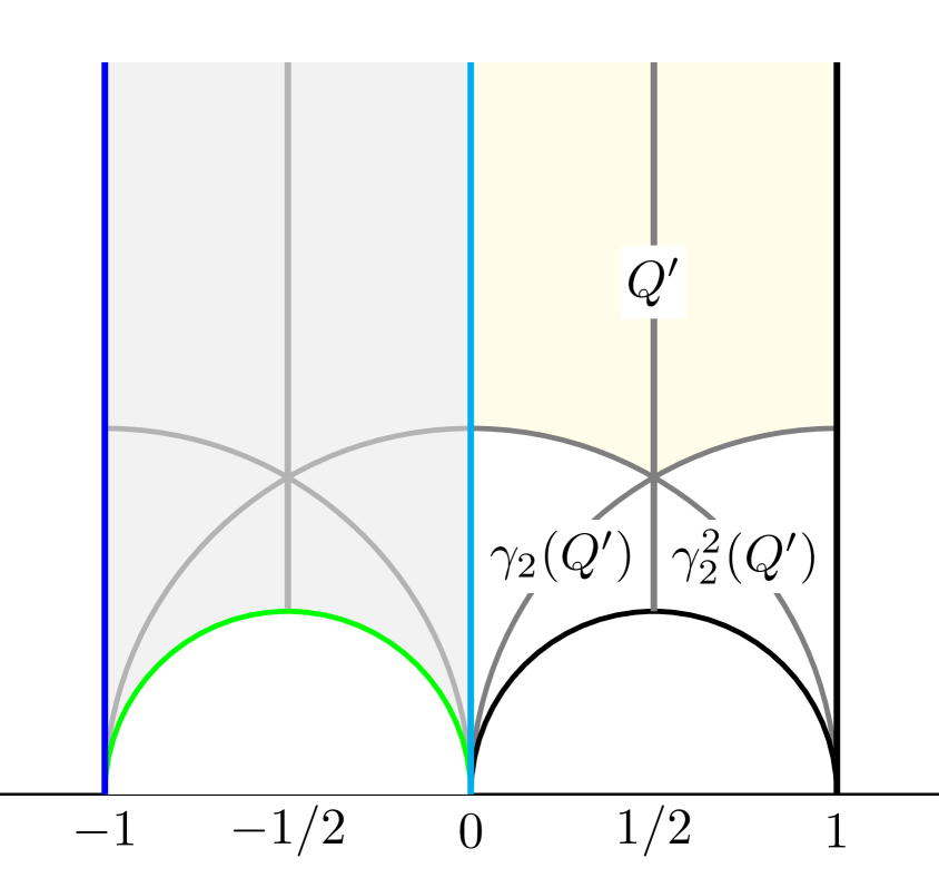
(a)

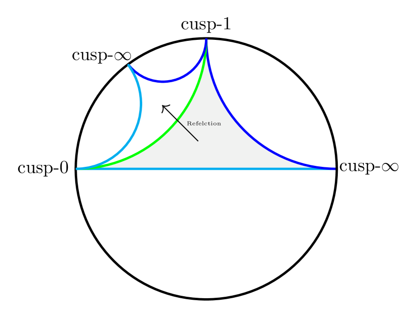
(b)

(c)

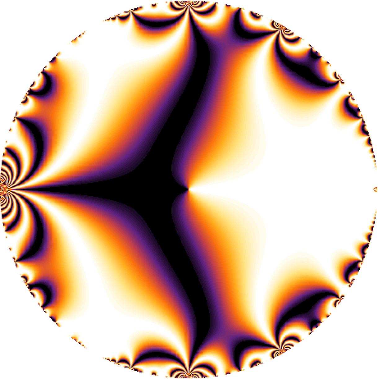
(d)

Figure 1: The hyperbolic tiling by triangle group $\Gamma_{\infty\infty\infty}$ and the modular function.

4.1 Uniformization of punctured $\mathbb{CP}^{1}$

By uniformization theorems [8], every Riemann surface is the quotient of either $\mathbb{H}\,,$ $\mathbb{C}\,,$ or $\mathbb{C}\mathbb{P}^{1}$ by a discrete group $\Gamma$ of automorphisms of $\mathbb{H}\,,$ $\mathbb{C}\,,$ or $\mathbb{C}\mathbb{P}^{1}$. Note that, in order for the action of $\Gamma$ to define a covering, $\Gamma$ must act freely, otherwise it is a branched covering. The universal cover of a (more than twice-) punctured $\mathbb{C}\mathbb{P}^{1}$ is $\mathbb{H}$. The reasoning is the following: it cannot be $\mathbb{C}\mathbb{P}^{1}$ since the latter is compact. Furthermore, the discrete and freely-acting subgroup of Aut($\mathbb{C}$) is a free abelian group with one or two generators. Thus $\mathbb{C}$ is either a covering of a twice punctured Riemann sphere, or a torus. All remaining Riemann surfaces are essentially isomorphic to $\Gamma\backslash\mathbb{H}$.

4.1.1 Poincaré polygon theorem

We start with the uniformization of the thrice-punctured Riemann sphere $\mathbb{CP}^{1}\setminus\Sigma$ with $\Sigma=\{0,1,\infty\}$. Our argument is based on the Poincaré polygon theorem [9, 10, 3], the Riemann mapping theorem and the Schwartz reflection principle. Starting from the gray hyperbolic triangle in fig. (1(a)1(b)) with zero angles at the three cusp points, we know from the Riemman mapping theorem that the interior of a triangle is conformally equivalent to the upper plane $\mathbb{H}$. We denote such a conformal map by $\lambda(\tau)$. It maps the boundary of the Schwartz triangle to the boundary of the upper half-plane $\mathbb{H}$, which is the real axis with punctures, ${\mathbb{R}}\setminus\Sigma$. By the Schwartz reflection principle, we can perform analytic continuation across the boundaries (see in fig. (1(b))), and the image will be the lower plane, because $\lambda(\tau)$ takes real values on the boundaries. The reflections can be generated by reflecting across $z=0\,,\lvert z-1/2\rvert=1/2$ and $z=1$ respectively, and the generators for the hyperbolic Todd-Coxeter group are

$$R_{1}(z)=-\overline{z}\,,\quad R_{2}(z)=\frac{\overline{z}}{2\overline{z}-1}\,,\quad R_{3}(z)=-\overline{z}+2\,.$$ (19)

These generators are anti-holomorphic Möbius transformations. We prefer another set of generators, which are holomorphic:

$$x_{1}(z)= R_{3}\circ R_{1}(z)=z+2\,,\quad\quad\text{fixes $\infty$}\,,$$

$$x_{2}(z)= R_{1}\circ R_{2}(z)=\frac{-z}{2z-1}\,,\quad\quad\text{fixes $0$}\,,$$

$$x_{3}(z)= R_{2}\circ R_{3}(z)=\frac{-z+2}{-2z+3}\,,\quad\quad\text{fixes $1$}\,.$$ (20)

Obviously, we have $x_{1}x_{2}x_{3}=1$, and they are the generators for the Fuchsian triangle group

$$\Gamma_{\infty,\infty,\infty}\equiv\langle x_{1}\,,x_{2}\,,x_{3}|x_{1}x_{2}x_{3}=1\rangle\,,$$ (21)

which are exactly the generators of the principal congruence subgroup $\Gamma(2)$, defined as follows

$$\Gamma(2)=\left\{\begin{pmatrix}a&b\\ c&d\end{pmatrix}\in\text{PSL}(2,\mathbb{Z})\,\,:\,\,\begin{pmatrix}a&b\\ c&d\end{pmatrix}\equiv\begin{pmatrix}1&0\\ 0&1\end{pmatrix}\,\,\text{mod}\,\,2\right\}\,.$$ (22)

Through iterative reflections, on the one hand by the Poincaré polygon theorem, the hyperbolic triangles will tessellate (fig. (1(c))) the Poincaré disk $\mathbb{D}$, and, on the other hand, $\lambda(\tau)$ is analytically continued to the whole Poincaré disk. So we conclude, the Poincaré disk $\mathbb{D}$ is the universal covering space of thrice-punctured $\mathbb{CP}^{1}\setminus\Sigma$, with $\lambda(\tau)$ the corresponding covering map. Again, from the Schwartz reflection principle, it is easy to see that $\lambda(\gamma\cdot\tau)=\lambda(\tau)\,,\forall\gamma\in\Gamma(2)$, so $\lambda$ descends to a well-defined bijective holomorphic map $\tilde{\lambda}$ from the modular curve $\Gamma(2)\backslash\mathbb{H}$ to $\mathbb{CP}^{1}\setminus\Sigma$. Its inverse is given by the ratio of the multi-valued period functions.

4.1.2 Torsion data from monodromy group

Consider the family of elliptic curves $E[2]$ given by eq. (8), of which the corresponding $j$ invariant is $j(\lambda)=256\frac{(1-\lambda(1-\lambda))^{3}}{\lambda^{2}(1-\lambda)^{2}}$. The $j$-invariant is ramified at $\lambda=\{0\,,1\,,\infty\}$, each with ramification index $2$, so that deg$j=6$. This coincides with the index $[\text{PSL}(2,\mathbb{Z})\,:\,\Gamma(2)]$ of $\Gamma(2)$ in $\text{PSL}(2,\mathbb{Z})$ (see fig. (1(a))). This shows that the family of elliptic curves carries extra information other than the shape encoded in $\tau$. The extra information turns out to be relevant torsion data for the congruence subgroup $\Gamma(2)$, and $E[2]$ is a family of elliptic curves attached to the moduli space $\mathscr{M}_{1;1}[2]$ [11].

The extra torsion data can be uncovered by computing the monodromy group for the corresponding Picard-Fuchs differential equation:

$$\left[4\lambda(1-\lambda)\frac{d^{2}}{d\lambda^{2}}+4(1-2\lambda)\frac{d}{d\lambda}-1\right]\Psi_{i}=0\,,\quad i=1\,,2.$$ (23)

The solution space is $\mathbb{C}\Psi_{1}(\lambda)\oplus\mathbb{C}\Psi_{2}(\lambda)$. It is a vector bundle over $\mathbb{CP}^{1}\setminus{\Sigma}$. By considering analytic continuation with a fixed base point, or equivalently the monodromy action [13, 3] by the base space fundamental group $\pi_{1}(B\,,\cdot)=\mathbb{Z}*\mathbb{Z}$, where $B=\mathbb{CP}^{1}\setminus{\Sigma}$, we have

$$\vec{\Psi}{\circlearrowleft}(\lambda)=\rho_{[\gamma]}\cdot\vec{\Psi}(\lambda)\,~{}~{}~{}\textrm{with}~{}~{}~{}\rho_{[\gamma_{1}][\gamma_{2}]}=\rho_{[\gamma_{1}]}\cdot\rho_{[\gamma_{2}]}\,.$$ (24)

And the images of $\pi_{1}(B\,,\cdot)$ under the homeomorphism

$$\begin{split}\rho:\pi_{1}(B\,,\cdot)&\,\to\textrm{GL}_{2}(\mathbb{C})\,\\ [\gamma]&\,\mapsto\rho_{[\gamma]}\end{split}$$ (25)

turn out to be the two free generators of $\Gamma(2)\lhd\mathbb{P}\text{SL}(2,\mathbb{Z})$

$$\rho_{[{\circlearrowleft}_{0}]}=\begin{pmatrix}1&2\\ 0&1\end{pmatrix}\,,\quad\rho_{[{\circlearrowleft}_{1}]}=\begin{pmatrix}1&0\\ -2&1\end{pmatrix}\,.$$ (26)

By the definition of $\tau$ in eq. (15), we see that analytic continuation induces a modular transformation

$$\tau_{\circlearrowleft}=\frac{a\tau+b}{c\tau+d}\equiv\gamma\cdot\tau\,,\quad\tau\in\mathbb{H}\,,\quad\gamma\in\Gamma(2)\,.$$ (27)

Moreover,

$$\Psi_{1\circlearrowleft}(\lambda)=c\Psi_{2}(\lambda)+d\Psi_{1}(\lambda)=(c\tau+d)\Psi_{1}(\lambda)\,,$$ (28)

so the period is a modular form of weight 1. Indeed, by the pull back of $\lambda$

$$\quad\Psi_{1}(\tau)=4\lambda^{*}(\operatorname{K})(\tau)=4\operatorname{K}(\lambda(\tau))=2\pi\theta_{3}^{2}(\tau)\,.$$ (29)

This is how period functions are related to modular forms.

4.1.3 Algebraic realization of the universal family of complex tori $\mathcal{E}_{\Gamma(2)\backslash{\mathbb{H}}}$

As a summary of the previous subsections, we have established the following relations:

(30)

with $\mathrm{Deck}_{\lambda}(\mathbb{H}\,,B=\mathbb{CP}^{1}\setminus\Sigma)\simeq\mathrm{Mono}\simeq\pi_{1}(B\,,\cdot)\simeq\Gamma(2)\simeq\mathbb{Z}*\mathbb{Z}$. Based on the previous observations, we will establish a equivalence between $\mathcal{E}_{\Gamma(2)\backslash{\mathbb{H}}}\equiv\left(\mathbb{Z}^{2}\rtimes\Gamma(2)\right)\backslash\left(\mathbb{C}\times{\mathbb{H}}\right)$ and the following family of elliptic curves

$$E_{\tau}[2]:Y^{2}=X(X-1)(X-\lambda(\tau))\,,\quad\tau\in\Gamma(2)\backslash\mathbb{H}\,,$$ (31)

which is conformally equivalent to $E[2]$ given by eq. (8). To this end, we utilize the Abel maps from $\mathcal{E}_{\Gamma(2)\backslash{\mathbb{H}}}$ to $E_{\tau}[2]$, given by $f_{[2]}$

$$(z,\tau)\in\mathcal{E}_{\Gamma(2)\backslash{\mathbb{H}}}\stackrel{{\scriptstyle f_{[2]}}}{{\longmapsto}}\left[X:\frac{1}{\Psi_{1}(\tau)}\partial{X}/{\partial z}:1\right]\in E_{\tau}[2]\,,$$ (32)

where after uniformization, the modular weight-1 period $\Psi_{1}(\tau)$ with respect to $\Gamma(2)$ is given in eq. (29). The isomorphism bwtween $\mathcal{E}_{\Gamma(2)\backslash{\mathbb{H}}}$ and $E[2]$ is given here by two equations

$$X(z,\tau)=\frac{\theta^{2}_{2}(\tau)\theta^{2}_{4}(z,\tau)}{\theta^{2}_{3}(\tau)\theta^{2}_{1}(z,\tau)}\,,\quad\lambda(\tau)=\frac{\theta_{2}^{4}(\tau)}{\theta_{3}^{4}(\tau)}\,.$$ (33)

The function $f_{[2]}$ defined through eq. (33) is invariant under the action of the semi-direct product $\mathbb{Z}^{2}\rtimes\Gamma(2)$,

$$f_{[2]}[z\,,\tau]=f_{[2]}[((m,n),\gamma)\cdot(z\,,\tau)]\,,\quad\forall(m\,,n)\in\mathbb{Z}^{2}\,,\gamma\in\Gamma(2)\,,$$ (34)

with $((m,n),\gamma)\cdot(z\,,\tau)=\left(\frac{z+m\tau+n}{c\tau+d}\,,\gamma\cdot\tau\right)$. Thus, $f_{[2]}$ is a well-defined holomorphic map between $\mathcal{E}_{\Gamma(2)\backslash{\mathbb{H}}}$ and $E[2]$. The map is bijective, its inverse is given by a family of Abel maps, we say $E[2]$ is an algebraic realization of the universal curve $\mathcal{E}_{\Gamma(2)\backslash{\mathbb{H}}}$.

4.2 Uniformization of the punctured $\mathbb{CP}^{2}$

4.2.1 Canonical coordinates on moduli space $\mathscr{M}_{1;2}[4]$

We want to generalize the story from the previous section to higher dimensions, where the base space is given by $\mathbb{CP}^{2}\setminus\Sigma$, with $\Sigma$ given in eq. (13). Intuition from lower dimensions tells us that the base should be isomorphic to some moduli space, which encodes the shape $\tau$ of the curves and the associated arithmetic data. Inspired by the Mordell-Weil theorem, which states that rational points on an elliptic curve form a finitely-generated abelian group $T_{\text{torsion}}\oplus r\mathbb{Z}$, we propose that the marked points should be given by the generator of Mordell-Weil group for the family of elliptic curves $E_{\textrm{bhabha}}$. We denote such a generator on $E_{\textrm{bhabha}}$ by $p_{0}$ with coordinates given by

$$\left[\frac{(s-4m^{2})s}{-4m^{2}+2s+t}:\,\frac{(s-4m^{2})s/m^{2}(s+t-4m^{2})}{(2s+t-4m^{2})^{2}/(s+t)}:\,m^{2}\right]\,.$$ (35)

The corresponding rational sections generated by $p_{0}$ are:

$$\{[n]p_{0}|\,p_{0}\in T_{\text{torsion}}\oplus r\mathbb{Z}\,,n\in\mathbb{Z}\}\simeq(\mathbb{Z}\,,+)\,.$$ (36)

We relabel $E_{\textrm{bhabha}}$ by canonical coordinates $(z\,,\tau)$. The variable $\tau$ indicates the shape of the curve, with possible level structures that encodes the torsion data [11]. The variable $z$ indicates the infinite subgroup $(\mathbb{Z}\,,+)$ of the Mordell-Weil group for a family of elliptic curves. This gives us two equations

$$\begin{split}\emph{Abel map:}\quad&\frac{(e_{2}-e_{4})(e_{1}-X)}{(e_{1}-e_{4})(e_{2}-X)}=\frac{\theta_{2}^{2}(\tau)}{\theta_{3}^{2}(\tau)}\frac{\theta_{1}^{2}(z,\tau)}{\theta_{4}^{2}(z,\tau)}\,,\\ \emph{Modular $\lambda$:}\quad&\frac{4}{2+\sqrt{\frac{-\mathrm{s}(\mathrm{s}+\mathrm{t}-4)}{-\mathrm{t}}}}=\frac{\theta_{2}^{4}(\tau)}{\theta_{3}^{4}(\tau)}\,,\end{split}$$ (37)

where $e_{i}$ are the four roots of $E_{\textrm{bhabha}}$ given in eq. (12). The $X$-coordinate is $X=\mathrm{s}(\mathrm{s}-4)/(-4+2\mathrm{s}+\mathrm{t})$. The Mandelstam variables $\textrm{s}=s/m^{2}$ and $\textrm{t}=t/m^{2}$ can be solved from eq. (37) as functions of $(z,\tau)$:

$$\textrm{s}=-\frac{4(-1+R)\times(-2+\lambda)}{-2+\lambda+R\times\lambda}\,,\quad\textrm{t}=\frac{4(-1+R)\times R\times\lambda^{2}}{({-2+R\times\lambda})({-2+\lambda+R\times\lambda})}\,,$$ (38)

where $R$ is given by the Abel map and $\lambda$ is the modular $\lambda$ function where

$$R=\frac{\theta_{2}^{2}(\tau)}{\theta_{3}^{2}(\tau)}\frac{\theta_{1}^{2}(z,\tau)}{\theta_{4}^{2}(z,\tau)}\,,\quad\lambda=\frac{\theta_{2}^{4}(\tau)}{\theta_{3}^{4}(\tau)}\,.$$ (39)

Note that $(\textrm{s}\,,\textrm{t})$ as functions of $(z\,,\tau)$ are invariant under the Hecke subgroup of $\Gamma_{0}(2)=\Gamma_{1}(2)>\Gamma_{1}(4)$.

With the same idea one can reparametrize the family of elliptic curves for top quark production in eq. (17). We found, after uniformization, a striking equivalence

$$\Psi_{\mathrm{bhabha}}\left(z,\tau\right)=\Psi_{\mathrm{tquark}}(z,\tau)=\frac{\pi\theta_{2}^{2}(\tau)}{2}\frac{\theta_{3}(z,\tau)\theta_{4}(z,\tau)}{\theta_{1}(z,\tau)\theta_{2}(z,\tau)}\,,\,\,$$ (40)

which is a modular function of weight 1 with respect to the semidirect product $\mathbb{Z}^{2}\rtimes\Gamma_{1}(4)$,

$$\Psi_{\mathrm{bhabha}}=\left(\frac{z+m\tau+n}{c\tau+d},\gamma\cdot\tau\right)=\frac{1}{c\tau+d}\Psi_{\mathrm{bhabha}}\left(z,\tau\right)\,,\quad\forall\gamma\in\Gamma_{1}(4)\,.$$ (41)

Based on these observations, we argue that the base space $\mathbb{C}\mathbb{P}^{2}\setminus\Sigma$ is biholomorphic to the quotient space of the universal covering space $\mathbb{C}\times\mathbb{H}$ modulo the action of the uniformization group $\mathbb{Z}^{2}\rtimes\Gamma_{1}(4)$:

(42)

4.2.2 The pullback of the symbol letters for Bhabha

We list several non-trivial closed 1-forms for Bhabha scattering and show their pullbacks. The first two are the fundamental 1-forms,

$$\omega_{\tau}= \frac{\mathrm{d}\mathrm{t}\,(\mathrm{s}-4)\mathrm{s}-\mathrm{d}\mathrm{s}\,\mathrm{t}(2\mathrm{s}+\mathrm{t}-4)}{2\mathrm{s}\mathrm{t}^{2}(\mathrm{s}-4)(\mathrm{s}+\mathrm{t}-4)(\mathrm{s}+\mathrm{t})\Psi_{1}^{2}(\mathrm{s},\mathrm{t})}\,,$$

$$\omega_{z}= \mathrm{d}\mathrm{t}\,\frac{-1}{4\mathrm{t}^{2}(\mathrm{s}+\mathrm{t}-4)(\mathrm{s}+\mathrm{t})}\frac{\mathrm{T}_{1}(\mathrm{s},\mathrm{t})}{\Psi_{1}^{2}(\mathrm{s},\mathrm{t})}$$

$$+ \mathrm{d}\mathrm{s}\bigg{(}\frac{2\mathrm{s}+\mathrm{t}-4}{4\mathrm{s}(\mathrm{s}-4)\mathrm{t}(\mathrm{s}+\mathrm{t})(\mathrm{s}+\mathrm{t}-4)}\frac{\mathrm{T}_{1}(\mathrm{s},\mathrm{t})}{\Psi_{1}^{2}(\mathrm{s},\mathrm{t})}+\frac{2\sqrt{-\mathrm{t}}\sqrt{4-\mathrm{t}}}{\mathrm{s}(\mathrm{s}-4)\mathrm{t}(\mathrm{t}-4)}\frac{1}{\Psi_{1}(\mathrm{s},\mathrm{t})}\bigg{)}\,,$$ (43)

where the integral over the period is defined as

$$\mathrm{T}_{1}(\mathrm{s},\mathrm{t})= \int\mathrm{d}\mathrm{s}\,\bigg{[}\frac{-\mathrm{t}}{\mathrm{s}}\frac{4\mathrm{s}^{2}+4\mathrm{s}(\mathrm{t}-4)+\mathrm{t}(\mathrm{t}-4)}{\sqrt{-\mathrm{t}}\sqrt{4-\mathrm{t}}}\Psi_{1}-8\mathrm{t}\frac{(\mathrm{s}+\mathrm{t}-4)(\mathrm{s}+\mathrm{t})}{\sqrt{-\mathrm{t}}\sqrt{4-\mathrm{t}}\,(t+2\mathrm{s}-4)}\partial_{\mathrm{s}}\Psi_{1}\bigg{]}$$

$$+ \mathrm{d}\mathrm{t}\bigg{[}\frac{-\mathrm{t}}{4-\mathrm{t}}\frac{-48+4\mathrm{s}+2\mathrm{s}^{2}+12\mathrm{t}+\mathrm{s}\mathrm{t}}{\sqrt{-\mathrm{t}}\sqrt{4-\mathrm{t}}\,(\mathrm{t}+\mathrm{s}-4)}\Psi_{1}\bigg{]}\,,\quad\text{~{}~{}with~{}~{}}\Psi_{1}=\pi\sqrt{-\mathrm{t}}\sqrt{4-\mathrm{t}}\Psi_{\mathrm{bhabha}}\,.$$ (44)

And a non-trivial depending on the integral $\mathrm{T}_{1}(\mathrm{s},\mathrm{t})$,

$$\omega_{41}= \,\mathrm{d}\mathrm{t}\bigg{[}\,\frac{1}{2\mathrm{t}^{2}(\mathrm{s}+\mathrm{t}-4)(\mathrm{s}+\mathrm{t})}\frac{\mathrm{T}_{1}^{2}(\mathrm{s},\mathrm{t})}{\Psi_{1}^{2}(\mathrm{s},\mathrm{t})}+\frac{2(\mathrm{s}-4)}{(\mathrm{t}-4)(\mathrm{s}+\mathrm{t}-4)}\bigg{]}+\,\mathrm{d}\mathrm{s}\bigg{[}-\frac{2\mathrm{t}(2\mathrm{s}^{2}+\mathrm{s}\mathrm{t}+4\mathrm{s}+12\mathrm{t}-48)}{(\mathrm{s}-4)\mathrm{s}(\mathrm{t}-4)(\mathrm{s}+\mathrm{t}-4)}$$

$$+ \frac{2\mathrm{s}+\mathrm{t}-4}{2(\mathrm{s}-4)\mathrm{s}\mathrm{t}(\mathrm{s}+\mathrm{t}-4)(\mathrm{s}+\mathrm{t})}\frac{\mathrm{T}_{1}^{2}(\mathrm{s},\mathrm{t})}{\Psi_{1}^{2}(\mathrm{s},\mathrm{t})}+\frac{\sqrt{\mathrm{t}(\mathrm{t}-4)}}{(s-4)\mathrm{s}(4-\mathrm{t})\mathrm{t}}\frac{\mathrm{T}_{1}(\mathrm{s},\mathrm{t})}{\Psi_{1}(\mathrm{s},\mathrm{t})}\bigg{]}\,.$$ (45)

The following results show the magic effect of the map given in eq. (38),

$$\omega_{\tau}\xmapsto{~{}f^{*}}i\pi\mathrm{d}\tau\textrm{~{}~{}~{}and~{}~{}~{}}\omega_{z}\xmapsto{~{}f^{*}}2\pi\mathrm{d}z\,,$$ (46)

and also the example with non-trivial connections to Kronecker’s differential forms [14, 15, 16],

$$\omega_{41}\xmapsto{~{}f^{*}}8\omega_{2}^{\text{Kro }}(2z\,,\tau)-8\omega_{2}^{\text{Kro}}(2z\,,2\tau)+\frac{4}{3}\frac{\mathrm{d}q}{q}\Theta_{D_{4}}(q^{2})\,,$$ (47)

where $q=e^{i\pi\tau}$ and the $\theta$-series of the $D_{4}$ root lattice is given by

$$\Theta_{D_{4}}(q^{2})=\theta_{3}^{4}(2\tau)+\theta_{2}^{4}(2\tau)\in\mathcal{M}_{2}(\Gamma_{0}(2))\subset\mathcal{M}_{2}(\Gamma_{1}(4))\,.\,\,\,$$ (48)

4.2.3 Algebraic realization of Kronecker’s differential forms

In section (4.1.3), we showed the family of elliptic curves $E[2]$ with level structure for $\Gamma(2)$ is equivalent to a universal family of complex tori $\mathcal{E}_{\Gamma(2)\backslash{\mathbb{H}}}$. The periods are modular forms of weight 1 on $\mathcal{E}_{\Gamma_{1}(4)\backslash{\mathbb{H}}}\equiv\left(\mathbb{Z}^{2}\rtimes\Gamma_{1}(4)\right)\backslash\left(\mathbb{C}\times{\mathbb{H}}\right)$. A natural question arises: what is the algebraic counterpart of $\mathcal{E}_{\Gamma_{1}(4)\backslash{\mathbb{H}}}$? That family of elliptic curves is

$$E_{t_{4}}:Y^{2}=(X^{2}-1)(X^{2}-t_{4})\,,$$ (49)

where $t_{4}\in\mathbb{CP}^{1}\setminus\Sigma$ with $\Sigma=\{0,1,\infty\}$. The omitted points are those when $E_{t_{4}}$ degenerates. The family of periods can be expressed in terms of complete elliptic integrals of the first kind, where

$$\begin{split}\Psi_{1}(t_{4})=\frac{4\operatorname{K}\left(\frac{4\sqrt{t_{4}}}{(1+\sqrt{t_{4}})^{2}}\right)}{1+\sqrt{t_{4}}}\,,\quad\Psi_{2}(t_{4})=\frac{4\operatorname{K}\left(1-\frac{4\sqrt{t_{4}}}{(1+\sqrt{t_{4}})^{2}}\right)}{1+\sqrt{t_{4}}}\,.\end{split}$$ (50)

The corresponding Picard-Fuchs operator describing a family of elliptic curves is:

$$\mathcal{L}:=\partial_{t_{4}}^{2}+\left(\frac{1}{t_{4}}-\frac{1}{1-t_{4}}\right)\partial_{t_{4}}+\frac{1}{4(t_{4}-1)t_{4}}\,.$$ (51)

The images of the generators of $\pi_{1}$ under the homeomorphism eq. (24) are given by

$$\rho_{[{\circlearrowleft}_{0}]}=\begin{pmatrix}1&1\\ 0&1\end{pmatrix}\,,\quad\rho_{[{\circlearrowleft}_{1}]}=\begin{pmatrix}1&0\\ -4&1\end{pmatrix}\,,$$ (52)

which are precisely the two candidate generators for the free group $\Gamma_{1}(4)$. Thus $\rho(\pi_{1}(X,\cdot))=\langle\rho_{[{\circlearrowleft}_{0}]}\,,\rho_{[{\circlearrowleft}_{1}]}\rangle=\Gamma_{1}(4)$. The Hauptmodul identifying $\mathbb{CP}^{1}\setminus\Sigma$ with $\Gamma_{1}(4)\backslash\mathbb{H}$ is [17]

$$t_{4}(\tau)=\left(\frac{\theta_{3}^{2}(\tau)-\theta_{4}^{2}(\tau)}{\theta_{3}^{2}(\tau)+\theta_{4}^{2}(\tau)}\right)^{2}\,.$$ (53)

Furthermore, the pullback of the period function by $t_{4}$ is given by

$$\Psi_{1}(\tau)=4\operatorname{K}(t_{4})=\pi(\theta_{3}^{2}(q)+\theta_{4}^{2}(q))=2\pi\theta^{2}_{3}(q^{2})=2\pi\frac{\eta^{10}(2\tau)}{\eta(\tau)\eta^{4}(4\tau)}\,,$$ (54)

indeed, it defines a modular form of weight 1 for $\Gamma_{1}(4)$, and note that dim$(\mathcal{M}_{1}(\Gamma_{1}(4)))=1$.

We establish the equivalence between $\mathcal{E}_{\Gamma_{1}(4)\backslash{\mathbb{H}}}$ and the following family of elliptic curves

$$E_{\tau}[4]:Y^{2}=(X^{2}-1)(X^{2}-t_{4}(\tau))\,,\quad\tau\in\Gamma_{1}(4)\backslash\mathbb{H}\,,$$ (55)

where $t_{4}(\tau)$ is the Hauptmodul for $\Gamma_{1}(4)$ given by eq. (53). We define a family of inverse Abel maps from $\mathcal{E}_{\Gamma_{1}(4)\backslash{\mathbb{H}}}$ to $E_{\tau}[4]$, given by $f_{[4]}$

$$(z,\tau)\in\mathcal{E}_{\Gamma_{1}(4)\backslash{\mathbb{H}}}\stackrel{{\scriptstyle f_{[4]}}}{{\longmapsto}}\left[X:\frac{1}{\Psi_{1}(\tau)}\partial{X}/{\partial z}:1\right]\in E_{\tau}[4]\,,$$ (56)

where the period function $\Psi_{1}(\tau)$ is given in eq. (54) and the $X$-coordinate is given by

$$2\frac{\sqrt{t_{4}(\tau)}+X}{(\sqrt{t_{4}(\tau)}+1)(1+X)}=\frac{\theta_{2}^{2}(\tau)}{\theta_{3}^{2}(\tau)}\frac{\theta_{4}^{2}(z,\tau)}{\theta_{1}^{2}(z,\tau)}\,.$$ (57)

The function $f_{[4]}$ defined in eq. (57) is invariant under the action of $\mathbb{Z}^{2}\rtimes\Gamma_{1}(4)$,

$$f_{[4]}[z\,,\tau]=f_{[4]}[((m,n),\gamma)\cdot(z\,,\tau)]\,,\quad\forall(m\,,n)\in\mathbb{Z}^{2}\,,\gamma\in\Gamma_{1}(4)\,.$$ (58)

Thus, $f_{[4]}$ descends to a well-defined holomorphic map from $\mathcal{E}_{\Gamma_{1}(4)\backslash{\mathbb{H}}}$ to $E_{\tau}[4]\simeq E_{t_{4}}$. The map is bijective, its inverse is given by a family of Abel maps, we say $E_{t_{4}}$ is an algebraic realization of the universal curves $\mathcal{E}_{\Gamma_{1}(4)\backslash{\mathbb{H}}}$.

Here is a short summary: we have identified $(z\,,\tau)$ on $\mathcal{E}_{\Gamma_{1}(4)\backslash{\mathbb{H}}}=\left(\mathbb{Z}^{2}\rtimes\Gamma_{1}(4)\right)\backslash\left(\mathbb{C}\times{\mathbb{H}}\right)$ with $(X\,,t_{4})$ on $E_{t_{4}}$, through a biholomorphic map $\tilde{g}$ given by the Hauptmodul eq. (53) and the family of Abel maps in eq. (57):

(59)

The effect of such an isomorphism is twofold: First, we can reparametrize the Mandelstam variables for Bhabha using canonical coordinates $\left([x:Y:1]\,,t_{4}\right)\in E_{t_{4}}$

$$\mathrm{s}=2\frac{(1-x)(1+t_{4})}{t_{4}-x}\,,\quad\mathrm{t}=4\frac{t_{4}(1-x^{2})}{x^{2}-t_{4}^{2}}\,.$$ (60)

Unlike the parametrization in eq. (38), this transformation is fully algebraic. We can clearly see all the branches of the full set of the symbol letters, e.g. , we can compute the period of Bhabha scattering

$$\Psi_{\mathrm{bhabha}}(x,t_{4})=\frac{2(x^{2}-t_{4})}{-Y}\operatorname{K}(t_{4})\,,$$ (61)

where $\operatorname{K}(t_{4})$ is the unique modular form of weight one for $\Gamma_{1}(4)$ in eq. (54), and $Y$ is the $Y$-coordinate of the universal family of elliptic curves $E_{t_{4}}$ given by eq. (49). We can also compute again for the pullback of the symbol letters given in section 4.2.2:

$$\omega_{z}\mapsto\frac{\pi}{2\operatorname{K}(t_{4})}\left(\frac{\mathrm{d}x}{Y}+\mathcal{F}(x,t_{4})\mathrm{d}t_{4}\right)\,,\quad\omega_{\tau}\mapsto\frac{\pi^{2}}{8\operatorname{K}^{2}(t_{4})}\frac{1}{t_{4}(1-t_{4})}\mathrm{d}t_{4}\,,$$ (62)

$$\omega_{41}\mapsto \left[2\frac{1-x^{2}}{(1-t_{4})(t_{4}-x^{2})}+8(1-t_{4})t_{4}\mathcal{F}^{2}(x,t_{4})\right]\mathrm{d}t_{4}+16(1-t_{4})t_{4}\mathcal{F}(x,t_{4})\frac{\mathrm{d}x}{Y}\,,$$ (63)

where $\mathcal{F}(x,t_{4})$ is the $\tau$-derivative of the Abel maps

$$\mathcal{F}(x,t_{4})=\operatorname{K}(t_{4})\times\partial_{t_{4}}{\left[\frac{1}{\operatorname{K}(t_{4})}F\left(x|t_{4}\right)\right]}\,,\quad F\left(x|t_{4}\right)\equiv\int_{-1}^{x}\frac{dX}{\sqrt{(X^{2}-1)(X^{2}-t_{4})}}\,.$$ (64)

$\mathcal{F}(x,t_{4})$ is related to $Z_{4}(x,t_{4})$ for the eMPLs [15]

$$\mathcal{F}(x,t_{4})=\frac{1}{4t_{4}}\frac{Z_{4}(x,t_{4})}{\sqrt{t_{4}}-1}-\frac{xY}{2t_{4}(t_{4}-1)(x^{2}-t_{4})}\,.$$ (65)

On the other hand, we can have an algebraic realization of Kronecker’s differential forms, e.g. ,

$$2\pi i\omega^{\text{Kro}}_{3}(2z,\tau)\xmapsto{~{}\tilde{g}^{{-1}*}} \,\mathrm{d}x\operatorname{K}(t_{4})\left[\frac{16t_{4}^{2}(1-t_{4})^{2}}{Y}\mathcal{F}^{2}(x,t_{4})+\frac{8t_{4}(1-t_{4})^{2}x}{Y^{2}}\mathcal{F}(x,t_{4})-\frac{2}{3}\frac{1+t_{4}}{Y}\right]$$

$$+ \mathrm{d}t_{4}\operatorname{K}(t_{4})\left[\frac{16}{3}(1-t_{4})^{2}t_{4}^{2}\mathcal{F}^{3}(x,t_{4})+\frac{2}{3}(1+t_{4})\mathcal{F}(x,t_{4})+\frac{2}{3}\frac{x(x^{2}-1)}{Y(x^{2}-t_{4})}\right]\,.$$ (66)

5 Conclusion

We computed Bhabha scattering at two loops–an amplitude beyond genus $0$ in QED. We revealed underlying connections between this amplitude and the arithmetic geometry of elliptic curves. We gave unified descriptions for several sectors of Bhabha scattering and planar top quark production through canonical coordinates on the moduli space $\mathscr{M}_{1;2}[4]$. Finally, we established correspondence between the Kronecker’s differential forms and letters of eMPLs.

References

• [1] J. B. Conway, Functions of one complex variable, Grad. Texts Math. Vol. 11 (Springer, Cham, 1973).
• [2] O. Forster, Lectures on Riemann surfaces. Transl. from the German by Bruce Gilligan, Grad. Texts Math. Vol. 81 (Springer, Cham, 1981).
• [3] J. M. Lee, Introduction to topological manifolds, Grad. Texts Math. Vol. 202, 2nd ed. ed. (New York, NY: Springer, 2011).
• [4] J. M. Henn, Phys. Rev. Lett. 110, 251601 (2013), 1304.1806.
• [5] J. M. Henn and V. A. Smirnov, JHEP 11, 041 (2013), 1307.4083.
• [6] C. Duhr, V. A. Smirnov, and L. Tancredi, JHEP 09, 120 (2021), 2108.03828.
• [7] H. Müller and S. Weinzierl, JHEP 07, 101 (2022), 2205.04818.
• [8] H. M. Farkas and I. Kra, Riemann surfaces., Grad. Texts Math. Vol. 71, 2nd ed. ed. (New York etc.: Springer-Verlag, 1992).
• [9] S. Katok, Fuchsian Groups (University of Chicago Press, 1981), pp. 92–110.
• [10] E. Girondo and G. González-Diez, Introduction to compact Riemann surfaces and dessins d’enfants, Lond. Math. Soc. Stud. Texts Vol. 79 (Cambridge: Cambridge University Press, 2012).
• [11] F. Diamond and J. Shurman, A first course in modular forms, Grad. Texts Math. Vol. 228 (Berlin: Springer, 2005).
• [12] J. Broedel, C. Duhr, and N. Matthes, JHEP 02, 184 (2022), 2109.15251.
• [13] R. Miranda, Algebraic curves and Riemann surfaces, Grad. Stud. Math. Vol. 5 (Providence, RI: AMS, American Mathematical Society, 1995).
• [14] S. Weinzierl, Feynman Integrals (, 2022), 2201.03593.
• [15] J. Broedel, C. Duhr, F. Dulat, and L. Tancredi, JHEP 05, 093 (2018), 1712.07089.
• [16] D. Zagier, Inventiones mathematicae 104, 449 (1991).
• [17] R. S. Maier, On rationally parametrized modular equations, 2008, math/0611041.