A simple GPU implementation of spectral-element methods for solving 3D Poisson type equations on cartesian meshes

Abstract

It is well known since 1960s that by exploring the tensor product structure of the discrete Laplacian on Cartesian meshes, one can develop a simple direct Poisson solver with an $\mathcal{O}(N^{\frac{d+1}{d}})$ complexity in $d$-dimension. The GPU acceleration of numerically solving PDEs has been explored successfully around fifteen years ago and become more and more popular in the past decade, driven by significant advancement in both hardware and software technologies, especially in the recent few years. We present in this paper a simple but extremely fast MATLAB implementation on a modern GPU, which can be easily reproduced, for solving 3D Poisson type equations using a spectral-element method. In particular, it costs less than one second on a Nvidia A100 for solving a Poisson equation with one billion degree of freedoms.

1 Introduction

It is well known that the tensor product structure of the discrete Laplacian can be used to invert the Laplacian since 1960s [15]. This approach has been particularly popular for spectral and spectral-element methods [8, 17, 18, 12, 2]. In fact, this method can be used for any discrete Laplacian on a Cartesian mesh. In this paper, as an example, we focus on the $Q^{k}$ spectral-element method, which is equivalent to the classical continuous finite element method with Lagrangian $Q^{k}$ basis implemented with the $(k+1)$-point Gauss–Lobatto quadrature [16, 13]. Tensor based solvers naturally fit the design of graphic processing units (GPUs). The earliest successful attempts to accelerate the computation of high order accurate methods in scientific computing communities include nodal discontinuous Galerkin method [11] almost fifteen years ago. These pioneering efforts of GPU acceleration of high order methods, or even those ones published later such as [3] in 2013, often rely on intensive coding.

In recent years, the surge in computational demands from machine learning and neural network based approaches has led to the evolution of modern GPUs. Correspondingly, software technologies have advanced considerably, streamlining the utilization of GPU computing. The landscape of both hardware and software has dramatically transformed, differing substantially from what existed a decade or even just two years ago.

In this paper, we present a straightforward yet robust implementation of accelerating the spectral-element method for three-dimensional discrete Laplacian on modern GPUs. In particular, for a total number of degree of freedoms as large as $1000^{3}$, the inversion of the 3D Laplacian using an arbitrarily high order $Q^{k}$ spectral-element method, takes no more than one second on one Nvidia A100 GPU card with 80G memory. While this impressive computational speed is naturally contingent on the hardware, it is noteworthy that our approach is grounded in a minimalist MATLAB implementation, ensuring ease of replication. In the Appendix, we give a full MATLAB code for solving a 3D Poisson equation on a rectangular domain using $Q^{k}$ spectral-element method.

We emphasize that the ability of solving Poisson type equation fast can play an important role in many fields of science and engineering. In fact, a large class of time dependent nonlinear systems, after a suitable implicit-explicit (IMEX) time discretization, often reduces to solving Poisson type equations at each time step (see, for instance, [19]). Therefore, having a simple, accurate and very fast solver for Poisson type equations can lead to very efficient numerical algorithms on modern GPUs for these nonlinear systems which include, e.g., Allen-Cahn and Chan-Hillard equations and related phase-field models [19], nonlinear Schrödinger equations, Navier-Stokes equations and related hydro-dynamic equations through a decoupled (projection, pressure correction etc.) approach [7]. In particular, by using the code provided in the Appendix, one can build, with a relatively easy effort, very efficient numerical solvers on modern GPUs for these time dependent complex nonlinear systems.

The rest of the paper is organized as follows. In Section 2, we give the implementation details for 3D problems. In Section 3, we demonstrate the good performance of this simple implementation for equations including the Poisson equation, a variable coefficient elliptic problem solved by the preconditioned conjugate gradient descent using Laplacian as a preconditioner, as well as a Cahn–Hilliard equation. Although our focus in this paper remains on the spectral-element method for these particular equations, similar results can be obtained for other problems with the same tensor product structure, e.g., finite difference schemes in implementing the matrix exponential in the exponential time differencing [6] and spectral fractional Laplacian [4]. Some concluding remarks are given in Section 4.

2 A spectral-element method for Poisson type equations

To fix the idea, we describe the implementation details for solving the Poisson type equation

$$\alpha u-\Delta u=f,$$ (1)

with a constant coefficient $\alpha>0$ and homogeneous Neumann boundary conditions on a rectangular domain $\Omega$. We only consider the spectral-element method with continuous piecewise $Q^{k}$ polynomial basis on uniform rectangular meshes, and all integrals are approximated by $(k+1)$-point Gauss–Lobatto quadrature [14].

2.1 The spectral-element method in two dimensions

We first consider the two dimensional case. As shown in Figure 1, such quadrature points naturally define all degree of freedoms since a single variable polynomial of degree $k$ is uniquely determined by its values at $k+1$ points.

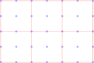
(a) A $3\times 2$ mesh for $Q^{2}$ element and the $3\times 3$ Gauss-Lobatto quadrature.

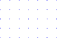
(b) All the quadrature points for $Q^{2}$ element.

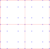
(c) A $2\times 2$ mesh for $Q^{3}$ element and the $4\times 4$ Gauss-Lobatto quadrature.

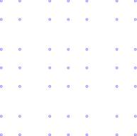
(d) All the quadrature points for $Q^{3}$ element.

Figure 1: An illustration of Lagrangian $Q^{k}$ element and the $(k+1)\times(k+1)$ Gauss-Lobatto quadrature.

On a rectangular mesh for $Q^{k}$ basis as shown in Figure 1 (a) or (c), let $(x_{i},y_{j})$ ($i=1,\cdots,N_{x};j=1,\cdots N_{y}$) denote all the points in Figure 1 (b) or (d). We consider the following finite element space of continuous piecewise $Q^{k}$ polynomials:

$$V^{h}=Span\{\phi_{i}(x)\phi_{j}(y),1\leq i\leq N_{x},1\leq j\leq N_{y}\},$$

where $\phi_{i}(x)$ ($i=1,\cdots,N_{x}$) denotes the $i$-th Lagrangian interpolation polynomial of degree $k$ in the $x$ direction as shown in Figure 1 (b) or (d).

Then, the $Q^{k}$ spectral-element method for solving (1) on a rectangular domain $\Omega$ is to seek $u_{h}\in V^{h}$ satisfying

$$\alpha\langle u_{h},v_{h}\rangle+\langle\nabla u_{h},\nabla v_{h}\rangle=\langle f,v_{h}\rangle,\quad\forall v_{h}\in V^{h},$$ (2)

where $\langle f,g\rangle$ denotes the approximation to the integral $\iint_{\Omega}f(x,y)g(x,y)\,dxdy$ by the $(k+1)\times(k+1)$ Gauss-Lobatto quadrature rule in each cell as shown in Figure 1.

The numerical solution $u_{h}(x,y)\in V^{h}$ can be expressed by the basis as

$$u_{h}(x,y)=\sum_{i=1}^{N_{x}}\sum_{j=1}^{N_{y}}u_{i,j}\phi_{i}(x)\phi_{j}(y),$$

where the coefficients $u_{i,j}=u_{h}(x_{i},y_{j})$ since $\phi_{i}(x)$ and $\phi_{j}(y)$ are chosen as the Lagrangian interpolation polynomials at $x_{i}$ and $y_{j}$.

Next, we define the one-dimensional stiffness matrix and the mass matrix as follows. The stiffness matrix $S_{x}$ is a matrix of size $N_{x}\times N_{x}$ with $(i,j)$-th entry being $\langle\phi^{\prime}_{i}(x),\phi^{\prime}_{j}(x)\rangle$. The mass matrix $M_{x}$ is a matrix of size $N_{x}\times N_{x}$ with $(i,j)$-th entry being $\langle\phi_{i}(x),\phi_{j}(x)\rangle$. The matrices $S_{y}$ and $M_{y}$ are similarly defined, with a size $N_{y}\times N_{y}$. Since the basis polynomials $\phi_{i}(\cdot)$ are Lagrangian interpolants at the quadrature points, the mass matrices $M_{x}$ and $M_{y}$ are diagonal.

Remark 1

Instead of the Lagrangian basis, we can also use the modal basis $L_{j}(x)-L_{j+2}(x)$ in each cell, where $L_{k}(x)$ is the Legendre polynomial of degree $k$, as the interior basis functions and the piecewise linear hat function at the intersecting points of two subintervals. This leads to sparse mass and stiffness matrices [12, 2].

Let $U$ be a matrix of size $N_{x}\times N_{y}$ with $u_{i,j}$ being its $(i,j)$-entry. Then $u_{h}(x,y)$ can be equivalently represented by the matrix $U$. Similarly, let $F$ be a matrix of size $N_{x}\times N_{y}$ with $f(x_{i},y_{j})$ being its $(i,j)$-entry. Then the scheme (2) can be equivalently written as

$$\alpha M_{x}UM^{T}_{y}+S_{x}UM^{T}_{y}+M_{x}US^{T}_{y}=M_{x}FM^{T}_{y}.$$ (3)

Detailed derivations of (3) can be found in [14, 20, 10].

2.2 The simple inversion by eigenvalue decomposition

For any matrix $X$ of size $m\times n$, define a vectorization operation $vec(\cdot)$, and let $vec(X)$ be the vector of size $mn$ obtained by reshaping all entries of $X$ into a column vector in a column by column order. Then for any two matrices $A_{1},A_{2}$ of proper sizes, it satisfies

$$vec(A_{1}XA_{2}^{T})=\left(A_{2}\otimes A_{1}\right)vec(X),$$ (4)

where $\otimes$ denotes the Kronecker product. With (4), the $Q^{k}$ spectral-element method (3) is also equivalent to

$$(\alpha M_{y}\otimes M_{x}+{M_{y}\otimes S_{x}+S_{y}\otimes M_{x}})vec(U)=(M_{y}\otimes M_{x})vec(F).$$ (5)

The linear system (3), or equivalently (5), can be solved by the following well-known method by using eigenvalue decomposition for only small matrices such as $S$ and $M$. For convenience, we only consider the simplified equivalent system

$$\alpha U+H_{x}U+UH^{T}_{y}=F,$$ (6)

or

$$(\alpha+{I_{y}\otimes H_{x}+H_{y}\otimes I_{x}})vec(U)=vec(F),$$ (7)

where $I$ is the identity matrix and $H=M^{-1}S$.

First, solve a generalized eigenvalue problem for small matrices $S$ and $M$, i.e., finding eigenvalues $\lambda_{i}$ and eigenvectors $\mathbf{v}_{i}$ satisfying

$$S\mathbf{v}_{i}=\lambda_{i}M\mathbf{v}_{i}.$$ (8)

Regardless of what kind of basis functions is used in a spectral-element method, the variational form of (2) ensures the symmetry of $S$ and $M$, thus a complete set of eigenvectors exists for (8). Let $\Lambda$ be a diagonal matrix with all eigenvalues $\lambda_{i}$ being diagonal entries, and let $T$ be the matrix with all corresponding eigenvectors $\mathbf{v}_{i}$ as its columns. Then

$$ST=MT\Lambda\Rightarrow H=M^{-1}S=T\Lambda T^{-1}.$$

Thus (7) becomes

$$[\alpha+{(T_{y}I_{y}T_{y}^{-1})\otimes(T_{x}\Lambda_{x}T_{x}^{-1})+(T_{y}\Lambda_{y}T_{y}^{-1})\otimes(T_{x}I_{x}T_{x}^{-1})}]vec(U)=vec(F),$$

which is equivalent to

$$(T_{y}\otimes T_{x})[\alpha+{I_{y}\otimes\Lambda_{x}+\Lambda_{y}\otimes I_{x}}](T_{y}^{-1}\otimes T_{x}^{-1})vec(U)=vec(F).$$ (9)

Notice that $\alpha+I_{y}\otimes\Lambda_{x}+\Lambda_{y}\otimes I_{x}$ is a diagonal matrix, thus its inverse is simple to compute. Let $\Lambda 2D$ be a matrix of size $N_{x}\times N_{y}$ with its $(i,j)$ entry being equal to $\alpha+(\Lambda_{x})_{i,i}+(\Lambda_{y})_{j,j}$, then (9) can be solved by

$$U=T_{x}[(T_{x}^{-1}FT_{y}^{-T})./\Lambda 2D]T_{y}^{T},$$ (10)

where $./$ denotes the entrywise division between two matrices.

Remark 2

In our spectral-element implementation, $M$ is diagonal. So we can consider an eigenvalue problem instead of the generalized eigenvalue problem (8). A numerically robust method, especially for very high order polynomial basis, is to solve the following symmetric eigenvalue problem. Let

$$H=M^{-1}S=M^{-1/2}(M^{-1/2}SM^{-1/2})M^{1/2}.$$

Since $S_{1}=M^{-1/2}SM^{-1/2}$ is real and symmetric, we can first find its eigenvalue decomposition as $S_{1}=Q\Lambda Q^{T}$ where $\Lambda$ is a diagonal matrix and $Q$ is an orthogonal matrix. Then, we have

$$H=M^{-1/2}(Q\Lambda Q^{T})M^{1/2}=T\Lambda T^{-1},$$

with $T=M^{-1/2}Q$ and $T^{-1}=Q^{T}M^{1/2}$. In Section 3.4, we will show numerical tests validating the robustness of this implementation for very high order elements.

2.3 Implementation for the three-dimensional case

On a three dimensional rectangualar mesh, any continuous piecewise $Q^{k}$ polynomial $u_{h}$ can be uniquely represented by a 3D array $U$ of size $N_{x}\times N_{y}\times N_{z}$ with $(i,j,k)$-th entry denoting the point value $u_{h}(x_{i},y_{j},z_{k})$, where $(x_{i},y_{j},z_{k})$ ($i=1,\cdots,N_{x};j=1,\cdots,N_{y};k=1,\cdots,N_{z}$) denotes all the quadrature points.

For a 3D array $U$, we define a page as the matrix obtained by fixing the last index of $U$. Namely, $U(\,:\,,\,:\,,k)$ for any fixed $k$ is a page of $U$. For a matrix $U(\,:\,,\,:\,,k)$ of size $N_{x}\times N_{y}$, recall that $vec(U(\,:\,,\,:\,,k))$ is a column vector of size $N_{x}N_{y}$. We define $\hat{U}$ as the following matrix of size $N_{x}N_{y}\times N_{z}$ obtained by reshaping $U$:

$$\hat{U}=\begin{bmatrix}vec(U(\,:\,,\,:\,,1))&vec(U(\,:\,,\,:\,,2))&\cdots&vec(U(\,:\,,\,:\,,N_{z}))\end{bmatrix}.$$

Then we define $vec(U)$ as the vector of size $N_{x}N_{y}N_{z}\times 1$ by reshaping $\hat{U}$ in a column by column order.

With the notation above, it is straightforward to verify that

$$(A_{3}^{T}\otimes A_{2}^{T}\otimes A_{1})vec(U)=vec((A_{2}^{T}\otimes A_{1})\hat{U}A_{3}).$$ (11)

Next, we consider how to implement the matrix vector multiplication in (11) without reshaping the 3D arrays. Let $Y$ be a 3D array of size $N_{x}\times N_{y}\times N_{z}$ defined by

$$vec(Y)=(A_{3}^{T}\otimes A_{2}^{T}\otimes A_{1})vec(U).$$ (12)

With the simple property (11), in our numerical tests, we find that the following simple implementation of (12) in MATLAB 2023 is efficient using two functions tensorprod and pagemtimes:

⬇

1% Computing a 3D array Y of the same size as U defined above= tensorprod(U,A3,3,1);

2Y = pagemtimes(Y,A2);

3Y = squeeze(tensorprod(A1,Y,2,1));

For the three-dimensional case, for simplicity, we consider the equation (1) with $\alpha=0$. With similar notation as in the two-dimensional case, the matrix form of the $Q^{k}$ spectral-element method (2) can be given as

$$\left(M_{z}\otimes M_{y}\otimes S_{x}+M_{z}\otimes S_{y}\otimes M_{x}+S_{z}\otimes M_{y}\otimes M_{x}\right)vec(U)$$

$$=\left(M_{z}\otimes M_{y}\otimes M_{x}\right)vec(F),$$

or equivalently,

$$\left(I_{z}\otimes I_{y}\otimes H_{x}+I_{z}\otimes H_{y}\otimes I_{x}+H_{z}\otimes I_{y}\otimes I_{x}\right)vec(U)=vec(F),$$ (13)

where $U$ is a 3D array with $(i,j,k)$-th entry denoting the point value $u_{h}(x_{i},y_{j},z_{k})$, and $F$ is a 3D array with $(i,j,k)$-th entry denoting the point value $f(x_{i},y_{j},z_{k})$.

With the eigenvalue decomposition $H=M^{-1}S=T\Lambda T^{-1}$, similar to the derivation of (9), the equation (13) is equivalent to

$$\leavevmode\resizebox{465.06001pt}{}{$(T_{z}\otimes T_{y}\otimes T_{x})\left(I_{z}\otimes I_{y}\otimes\Lambda_{x}+I_{z}\otimes\Lambda_{y}\otimes I_{x}+\Lambda_{z}\otimes I_{y}\otimes I_{x}\right)(T_{z}^{-1}\otimes T_{y}^{-1}\otimes T_{x}^{-1})vec(U)=vec(F)$}.$$ (14)

Define a 3D array $\Lambda 3D$ with its $(i,j,k)$-th entry being equal to $(\Lambda_{x})_{i,i}+(\Lambda_{y})_{j,j}+(\Lambda_{z})_{k,k}$, then (14) can be implemented efficiently as the following in MATLAB:

⬇

1% Simple and efficient implementation of (14)TInv denotes the inverse matrix of T

2U = tensorprod(F,TzInv',3,1);

3U = pagemtimes(U,TyInv');

4U = squeeze(tensorprod(TxInv,U,2,1));

5U = U./Lambda3D;

6U = tensorprod(U,Tz',3,1);

7U = pagemtimes(U,Ty');

8U = squeeze(tensorprod(Tx,U,2,1));

Table 1: The MATLAB 2023 script of implementing (14) on both CPU and GPU.

3 Numerical tests

In this section, we report the performance of the simple MATLAB implementation in Table 1. In particular, a demonstration code is provided in the Appendix. The performance and speed-up are of course dependent on the hardwares. We test our code on the following three devices:

1. CPU: Intel i7-12700 2.10 GHz (12-core) with 16G memory;

2. GPU: Quadro RTX 8000 (48G memory);

3. GPU: Nvidia A100 (80G memory).

In MATLAB 2023, for computation on either CPU or GPU, the code for implementing (14) is the same as in Table 1. On the other hand, matrices like $T_{x},T_{y},T_{z}$ and arrays like $F$ and $\Lambda 3D$ must be loaded to GPU memory before performing the GPU computation, see the full code in the Appendix. We define the process of loading matrices and arrays $T_{x},T_{y},T_{z},F,\Lambda 3D$ as the offline step since it is preparatory, and undertaken only once, regardless of how many times the Laplacian needs to be inverted. We define the step in Table 1 as the online computation step. All the computational time reported in this section are online computational time, i.e., we do not count the offline preparational time.

3.1 Accuracy tests

We list a few accuracy tests to show that the scheme implemented is indeed high order accurate. In particular, the $Q^{k}$ ($k\geq 2$) spectral-element method is $(k+2)$-th order accurate for smooth solutions when measuring the $\ell^{2}$ error in function values for solving second order PDEs, which has been rigorously proven recently in [14, 13].

We consider the Poisson type equation (1) with $\alpha=1$ in domain $\Omega=[-1,1]^{3}$. For Dirichlet boundary conditions, we test a smooth exact solution

$$u_{D}^{*}(\bm{x})=\sin(\pi x)\sin(2\pi y)\sin(3\pi z)+(x-x^{3})(y^{2}-y^{4})(1-z^{2}).$$

For Neumann boundary conditions, we test a smooth exact solution

$$u_{N}^{*}(\bm{x})=\cos(\pi x)\cos(2\pi y)\cos(3\pi z)+(1-x^{2})^{3}(1-y^{2})^{2}(1-z^{2})^{4}.$$

The results of $Q^{5}$ and $Q^{6}$ spectral-element methods are listed in Table 2.

$Q^{5}$ spectral-element method (SEM)
FEM Mesh	Dirichlet boundary			Neumann boundary
	Total DoFs	$\ell^{2}$ error	order	Total DoFs	$\ell^{2}$ error	order
$2^{3}$	$9^{3}$	$2.27$E-$1$	-	$11^{3}$	$4.76$E-$1$	-
$4^{3}$	$19^{3}$	$3.91$E-$3$	$5.86$	$21^{3}$	$5.49$E-$3$	$6.44$
$8^{3}$	$39^{3}$	$4.12$E-$5$	$6.57$	$41^{3}$	$4.32$E-$5$	$6.99$
$16^{3}$	$79^{3}$	$3.34$E-$7$	$6.95$	$81^{3}$	$3.42$E-$7$	$6.98$
$32^{3}$	$159^{3}$	$2.63$E-$9$	$6.99$	$161$	$2.67$E-$9$	$7.00$
$Q^{6}$ spectral-element method (SEM)
FEM Mesh	Dirichlet boundary			Neumann boundary
	Total DoFs	$\ell^{2}$ error	order	Total DoFs	$\ell^{2}$ error	order
$2^{3}$	$11^{3}$	$9.68$E-$2$	-	$13^{3}$	$1.18$E-$1$	-
$4^{3}$	$23^{3}$	$6.05$E-$4$	$7.32$	$25^{3}$	$8.42$E-$4$	$7.13$
$8^{3}$	$47^{3}$	$3.11$E-$6$	$7.60$	$49^{3}$	$3.24$E-$6$	$8.02$
$16^{3}$	$95^{3}$	$1.26$E-$8$	$7.95$	$97^{3}$	$1.28$E-$8$	$7.98$
$32^{3}$	$191^{3}$	$4.96$E-$11$	$7.98$	$193^{3}$	$5.09$E-$11$	$7.98$

Table 2: Accuracy tests for discrete Laplacian for a 3D problem with Dirichlet boundary conditions and a 3D problem with Neumann boundary conditions.

3.2 GPU acceleration for solving a Poisson type equation

In this subsection, we list the online computational time comparison for solving $\alpha u-\Delta u=f$ on $\Omega=[-1,1]^{3}$ with $\alpha=1$ and Neumann boundary conditions, by using the $Q^{5}$ spectral-element method. To obtain a more accurate estimate of the online computational time, we count the online computation time for solving the Poisson equation 200 times. The results of online computational time, depicted in Figure 2 and Table 3, demonstrate a speed-up factor of at least 60 for sufficiently large problems when comparing Nvidia A100 to Intel i7-12700. In particular, we observe that on the A100, solving a Poisson type equation (1) with a total degree of freedoms (DoFs) equal to $1001^{3}$, takes approximately only 0.8 second.

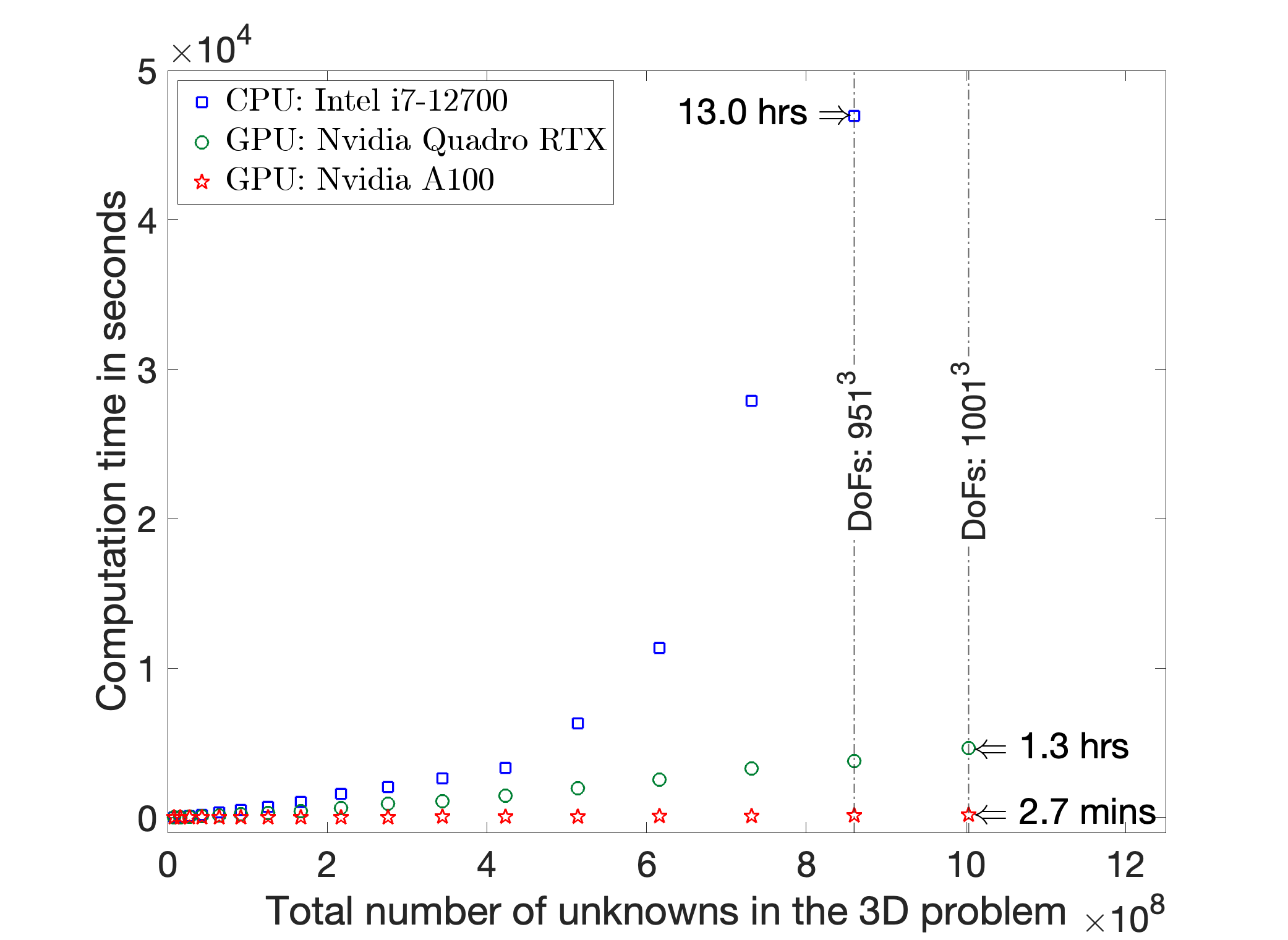
(a) Comparison on three devices.

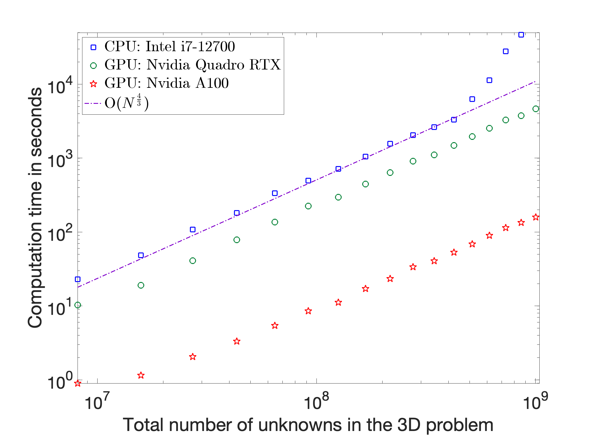
(b) Semilogx plot shows the complexity on all devices are $\mathcal{O}(N^{\frac{4}{3}})$ for problems with proper sizes.

Figure 2: Online computation time of $Q^{5}$ spectral-element method solving a 3D Poisson equation two hundred times. On the A100, it takes approximately only 0.8 second when solving one Poisson equation for the total number of DoFs being $1001^{3}$.

Total DoFs	Intel i7-12700	NVIDIA Quadro		NVIDIA A100
	CPU time	GPU time	speed-up	GPU time	speed-up
$201^{3}$	$2.29$E$1$	$1.03$E$1$	$2.23$	$9.00$E-$1$	$25.47$
$251^{3}$	$4.86$E$1$	$1.91$E$1$	$2.54$	$1.15$E$0$	$42.14$
$301^{3}$	$1.08$E$2$	$4.10$E$1$	$2.65$	$2.05$E$0$	$52.94$
$351^{3}$	$1.81$E$2$	$7.82$E$1$	$2.32$	$3.31$E$0$	$54.77$
$401^{3}$	$3.36$E$2$	$1.36$E$2$	$2.47$	$5.41$E$0$	$62.12$
$451^{3}$	$4.98$E$2$	$2.25$E$2$	$2.22$	$8.52$E$0$	$58.49$
$501^{3}$	$7.13$E$2$	$2.96$E$2$	$2.41$	$1.11$E$1$	$64.09$
$551^{3}$	$1.05$E$2$	$4.46$E$2$	$2.35$	$1.71$E$1$	$61.19$
$601^{3}$	$1.57$E$3$	$6.40$E$2$	$2.46$	$2.35$E$1$	$67.09$
$651^{3}$	$2.05$E$3$	$9.09$E$2$	$2.25$	$3.37$E$1$	$60.68$
$701^{3}$	$2.63$E$3$	$1.11$E$3$	$2.37$	$4.07$E$1$	$64.63$
$751^{3}$	$3.30$E$3$	$1.48$E$3$	$2.23$	$5.31$E$1$	$62.19$
$801^{3}$	$6.29$E$3$	$1.97$E$3$	$3.20$	$6.86$E$1$	$91.64$
$851^{3}$	$1.13$E$4$	$2.55$E$3$	$4.45$	$8.97$E$1$	$126.36$
$901^{3}$	$2.79$E$4$	$3.27$E$3$	$8.53$	$1.14$E$2$	$244.19$
$951^{3}$	$4.69$E$4$	$3.77$E$3$	$12.45$	$1.34$E$2$	$349.16$

Table 3: Online computation time of solving a 3D Poisson equation two hundred times on three devices: the time unit is second, and the speed-up is GPU versus CPU.

3.3 GPU acceleration for solving a Schrödinger equation

For a Problem with general variable coefficients, the tensor product structure of the eigenvectors no longer holds. Then, an efficient method for solving such problems is to use a preconditioned conjugate gradient method with the inverse of Poisson type equation as a preconditioner. As an example, we consider the following equation

$$\alpha u-\Delta u+V(\bm{x})u=f,$$ (15)

on $\Omega=[-16,16]^{3}$ with $\alpha=1$,

$$V(\bm{x})=\beta\sin(\frac{\pi}{4}x)^{2}\sin(\frac{\pi}{4}y)^{2}\sin(\frac{\pi}{4}z)^{2},\quad\beta>0,$$ (16)

and an exact solution

$$u(\bm{x})=\cos(\frac{\pi}{16}x)\cos(\frac{\pi}{16}y)\cos(\frac{\pi}{16}z).$$ (17)

The equation (15) is sometimes referred to as a Schrödinger equation, which emerges in solving more complicated problems originated from the nonlinear Schrödinger equation, e.g., the Gross-Pitaevskii equation [5]. The boundary conditions can be either periodic or homogeneous Neumann.

Note that $0\leq V(x)\leq\beta$. We use $((\alpha+\frac{1}{2}\beta)I-\Delta)^{-1}$ as a preconditioner in the preconditioned conjugate gradient (PCG) method inverting the operator $\alpha I-\Delta+V(\mathbf{x})$ with periodic boundary conditions in the $Q^{5}$ spectral-element method, where $((\alpha+\frac{1}{2}\beta)I-\Delta)^{-1}$ is implemented in the same way as in Table 1. We emphasize that eigenvectors can not be implemented by fast Fourier transform (FFT) for high order schemes with periodic boundary conditions, because the stiffness matrix $S$ for $Q^{k}$ SEM is a circulant matrix only when $k=1$, i.e., FFT can be used to invert Laplacian only for second order accurate schemes.

Obviously, the performance of such a simple method depends on the condition number of the operator $\alpha I-\Delta+V(\mathbf{x})$, which is affected by the choice of $V(\mathbf{x})$. By choosing different $\beta$ in (16), the performance of PCG, e.g., the number of PCG iterations needed for the PCG iteration residue to reach round-off errors, would vary. We first list the performance of PCG for the $Q^{5}$ spectral-element method on different meshes for different $\beta$ in Table 4. We can observe that the performance only depends on $V(\bm{x})$ for a fine enough mesh.

Total	Number of PCG iterations
DoFs	$\beta=1$	$10$	$100$	$200$	$400$	$800$	$1000$	$2000$	$4000$	$10000$
$250^{3}$	$10$	$35$	$85$	$112$	$149$	$191$	$214$	$288$	$388$	$535$
$350^{3}$	$10$	$32$	$81$	$108$	$143$	$184$	$202$	$265$	$348$	$522$
$450^{3}$	$10$	$30$	$80$	$105$	$142$	$181$	$191$	$252$	$333$	$467$
$550^{3}$	$10$	$28$	$76$	$104$	$129$	$174$	$183$	$239$	$321$	$448$
$650^{3}$	$10$	$27$	$77$	$100$	$135$	$169$	$182$	$248$	$327$	$465$
$750^{3}$	$10$	$27$	$76$	$100$	$130$	$173$	$192$	$233$	$320$	$456$
$850^{3}$	$10$	$27$	$76$	$100$	$134$	$173$	$188$	$233$	$305$	$430$
$950^{3}$	$10$	$25$	$72$	$98$	$128$	$165$	$180$	$234$	$305$	$428$
$1000^{3}$	$10$	$25$	$72$	$101$	$134$	$172$	$188$	$243$	$305$	$433$

Table 4: Number of PCG iterations needed for PCG with $((\alpha+\frac{1}{2}\beta)I-\Delta)^{-1}$ as the preconditioner to converge for solving a Schrödinger equation by the $Q^{5}$ SEM on different meshes with different $\beta=1,10,100,200,\cdots,10000$.

The online computational time of using PCG for the $Q^{5}$ spectral-element method solving one Schrödinger equation with $\beta=1$ in (16) is listed in both Figure 3 and Table 5. We can observe a satisfying speed-up. With 10 PCG iterations, it costs about $20$ seconds on A100 for inverting a 3D Schrödinger operator for a total number of DoFs as large as $1000^{3}$.

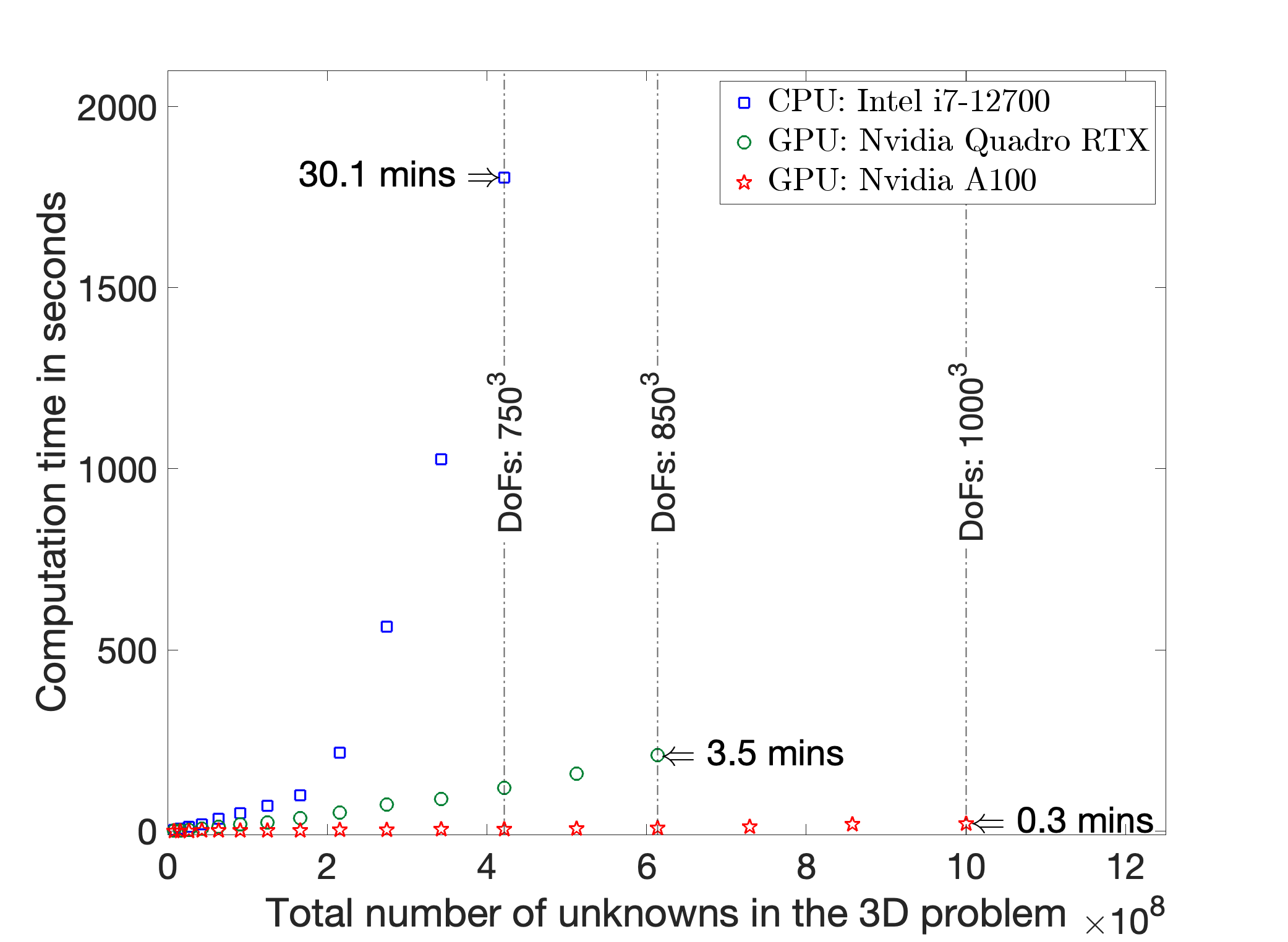
(a) Comparison on three devices.

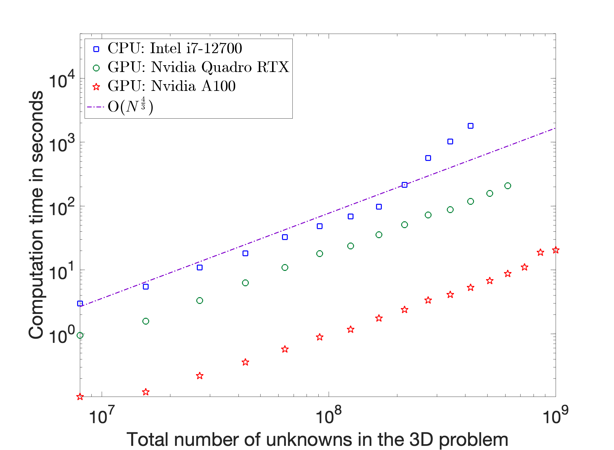
(b) Semilogx plot shows the complexity on all devices are $\mathcal{O}(N^{\frac{4}{3}})$ for problems of proper sizes.

Figure 3: Online computational time of $Q^{5}$ SEM for a Schrödinger equation with $\beta=1$ in (16), solved by PCG with $(I-\Delta)^{-1}$ as the preconditioner.

Total DoFs	$200^{3}$	$250^{3}$	$300^{3}$	$350^{3}$	$400^{3}$	$450^{3}$
Intel i7-12700	$2.99$E$0$	$5.50$E$0$	$1.09$E$1$	$1.81$E$1$	$3.27$E$1$	$4.83$E$1$
Nvidia Quadro	$9.48$E-$1$	$1.58$E$0$	$3.32$E$0$	$6.30$E$0$	$1.10$E$1$	$1.80$E$1$
Nvidia A100	$1.04$E-$1$	$1.23$E-$1$	$2.21$E-$1$	$3.61$E-$1$	$5.75$E-$1$	$8.86$E-$1$
Total DoFs	$500^{3}$	$550^{3}$	$600^{3}$	$650^{3}$	$700^{3}$	$750^{3}$
Intel i7-12700	$6.90$E$1$	$9.83$E$1$	$2.16$E$2$	$5.63$E$2$	$1.03$E$3$	$1.80$E$3$
Nvidia Quadro	$2.38$E$1$	$3.55$E$1$	$5.11$E$1$	$7.23$E$1$	$8.78$E$1$	$1.18$E$2$
Nvidia A100	$1.18$E$0$	$1.75$E$0$	$2.38$E$0$	$3.35$E$0$	$4.10$E$0$	$5.30$E$0$
Total DoFs	$800^{3}$	$850^{3}$	$900^{3}$	$950^{3}$	$1000^{3}$
Nvidia Quadro	$1.57$E$2$	$2.09$E$2$	-	-	-
Nvidia A100	$6.79$E$0$	$8.71$E$0$	$1.11$E$1$	$1.88$E$1$	$2.04$E$1$

Table 5: The online computational time (unit is second) of using PCG for the $Q^{5}$ SEM solving one Schrödinger equation with $\beta=1$ in (16).

3.4 Robustness of the implementation for very high order elements

For very high order elements, it is important to have a robust procedure for finding the eigenvalue decomposition of the matrix $H$. We test the implementation in Remark 2 for the $Q^{20}$ spectral-element method solving the Schrödinger equation. The error in Table 6 and the online computational time in Table 7 validate the robustness of the implementation. In other words, even for $Q^{20}$ element, the numerical computation of eigenvalue decomposition in Remark 2 is still accurate.

Total DoFs	$\ell^{\infty}$ error
	$\beta=1$	$\beta=10$	$\beta=100$
$500^{3}$	$1.89$E-$13$	$1.62$E-$13$	$1.29$E-$13$
$800^{3}$	$4.86$E-$13$	$4.09$E-$13$	$2.97$E-$13$
$1000^{3}$	$6.28$E-$13$	$5.23$E-$13$	$3.76$E-$13$

Table 6: The $\ell^{\infty}$ error for $Q^{20}$ SEM solving one Schrödinger equation with different $\beta$ in (16).

Total DoFs	$\beta=1$		$\beta=10$		$\beta=100$
	Time	$\#$ PCG	Time	$\#$ PCG	Time	$\#$ PCG
$500^{3}$	$1.23$E$0$	10	$2.36$E$0$	23	$6.47$E$0$	68
$800^{3}$	$7.13$E$0$	11	$3.15$E$1$	56	$7.84$E$1$	142
$1000^{3}$	$2.04$E$1$	10	$4.40$E$1$	23	$1.30$E$2$	70

Table 7: Online computational time in seconds for $Q^{20}$ SEM solving one Schrödinger equation with different $\beta$ in (16).

3.5 Comparison with FFT on GPU

It is also interesting to compare the implementation in Table 1 with the performance of fast Fourier transform (FFT) on GPU. In order to do so, we consider solving the Poisson type equation(1) and the Schrödinger equation (23) with periodic boundary conditions using second order finite difference, or equivalently the $Q^{1}$ spectral-element method, for which the discrete Laplacian can be diagonalized by FFT, e.g., the eigenvector matrices $T^{-1}$ in (14) is the discrete Fourier transform matrix. In other words, for $Q^{1}$ element with periodic boundary, the implementation in Table 1 can be replaced by the following implementation via FFT in MATLAB:

⬇

1 fftn(F);

2U = U./Lambda3D;

3U = real(ifftn(U));

Table 8: The FFT implementation of a second order scheme for the Poisson equation with periodic boundary conditions.

We will refer to such an implementation for a second order scheme as FFT in Figure 4 and Figure 5. On the other hand, even if the Poisson equation has periodic boundary conditions, the matrices $T$ and $T^{-1}$ for high order elements cannot be implemented by FFT. We simply refer to the implementation in Table 1 for high order elements as SEM in Figure 4 and Figure 5. The detailed comparison is listed in Figure 4 and Figure 5, as well as Table 9 and Table 10. We can observe that FFT is faster as expected, on most meshes. However, the memory cost of performing FFT is more demanding, especially on finer meshes. For the Schrödinger problem, the performance of FFT deteriorates on finest meshes.

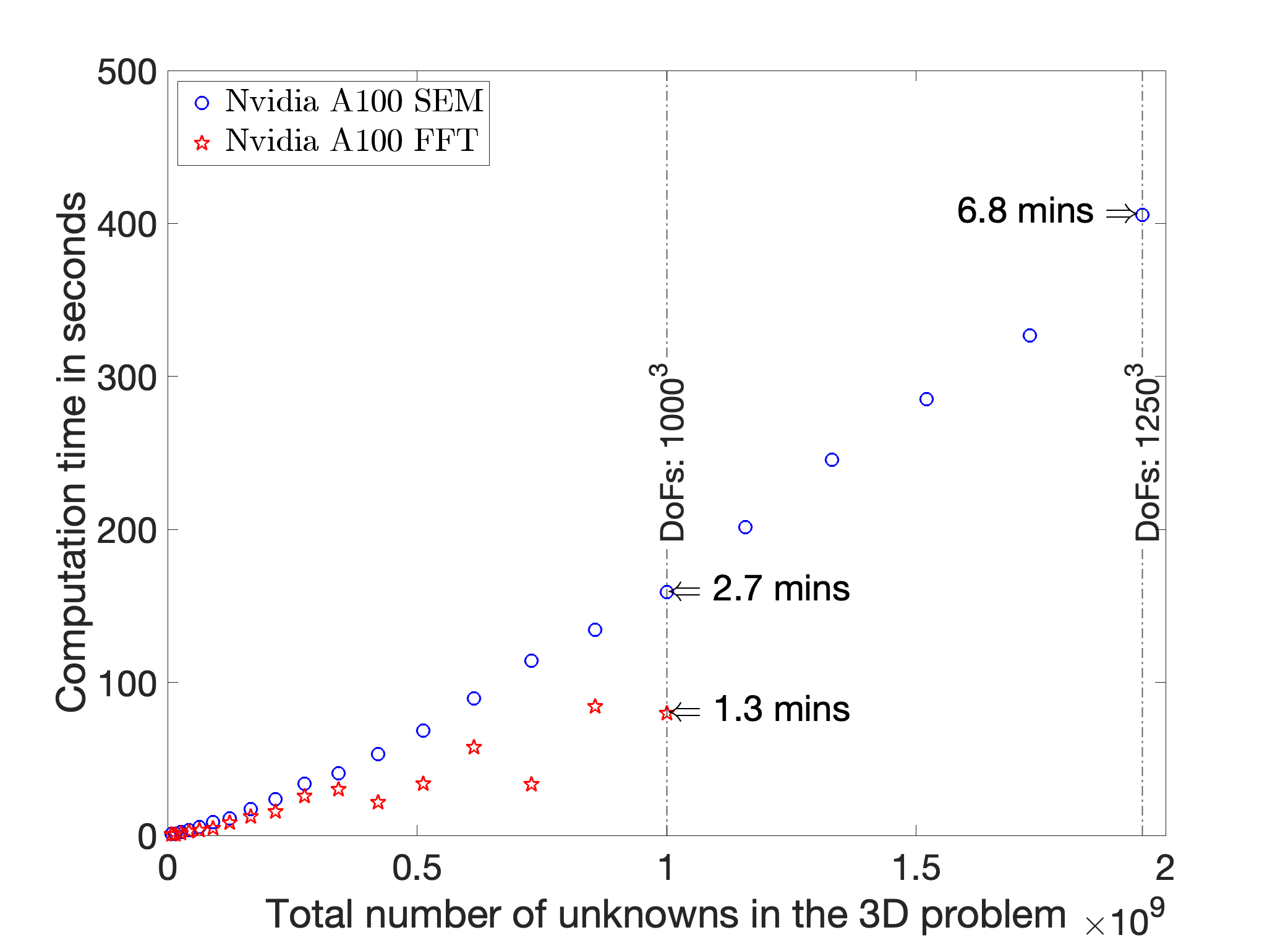
(a) Comparison on one device.

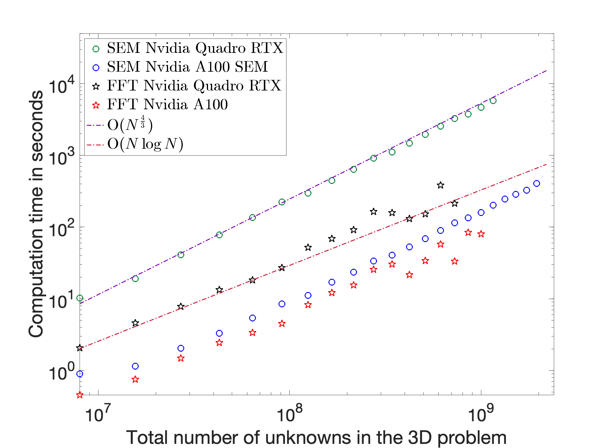
(b) Semilogx plot shows the complexity.

Figure 4: Comparison between $Q^{5}$ SEM implemented in Table 1 and a second order scheme implemented by FFT in Table 8, for solving a Poisson equation 200 times. On A100, the FFT implementation cannot solve a problem of size $1050^{3}$ in MATLAB 2023, due to the larger memory cost of FFT.

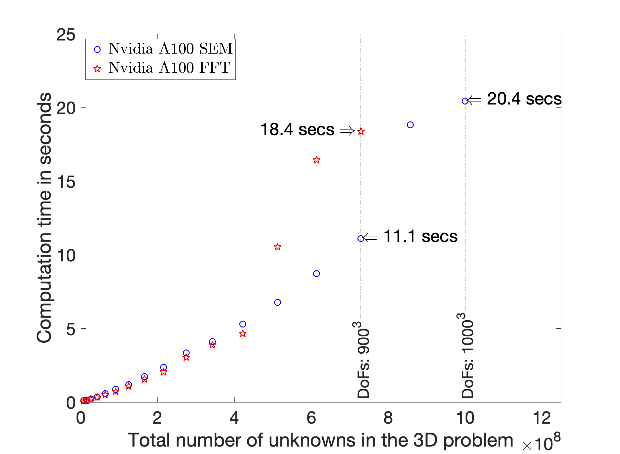
(a) Comparison on one device.

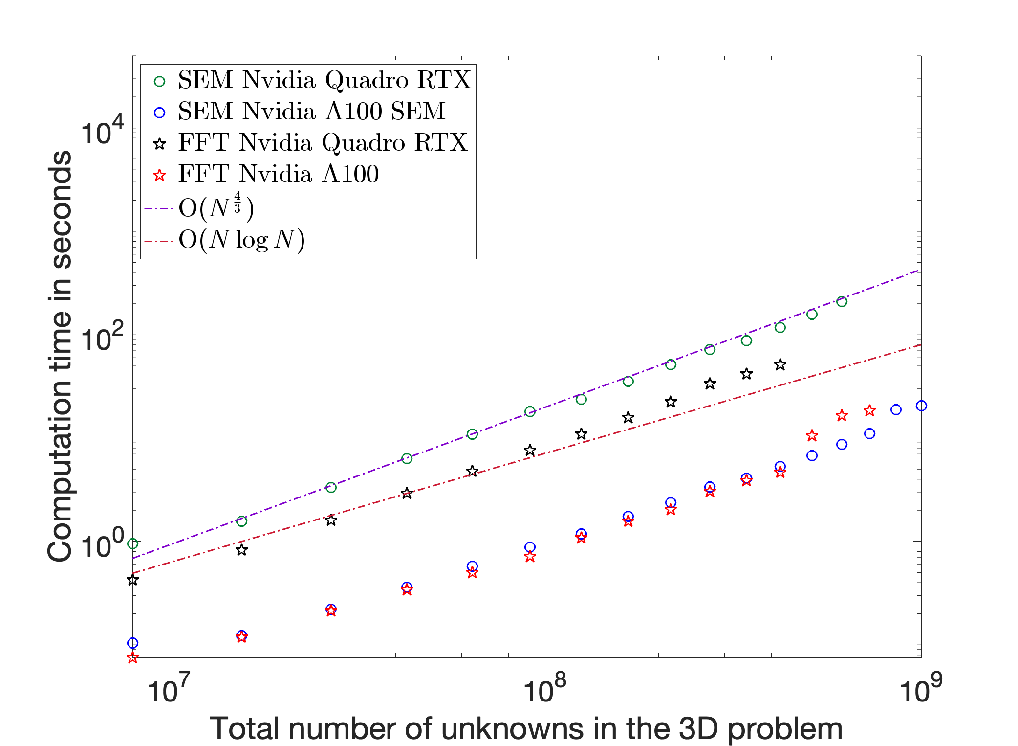
(b) Semilogx plot shows the complexity.

Figure 5: Comparison between $Q^{5}$ SEM implemented in Table 1 and a second order scheme implemented by FFT in Table 8 for solving a Schrödinger equation by PCG. On A100, the FFT implementation cannot solve a problem of size $950^{3}$ in MATLAB 2023, due to the larger memory cost of FFT.

Total DoFs	$200^{3}$	$250^{3}$	$300^{3}$	$350^{3}$	$400^{3}$	$450^{3}$
Quadro (SEM)	$1.03$E$1$	$1.91$E$1$	$4.10$E$1$	$7.82$E$1$	$1.36$E$2$	$2.25$E$2$
Quadro (FFT)	$2.06$E$0$	$4.61$E$0$	$7.82$E$0$	$1.33$E$1$	$1.83$E$1$	$2.70$E$1$
A100 (SEM)	$9.00$E-$1$	$1.15$E$0$	$2.05$E$0$	$3.31$E$0$	$5.41$E$0$	$8.52$E$0$
A100 (FFT)	$4.58$E-$1$	$7.50$E-$1$	$1.49$E$0$	$2.44$E$0$	$3.37$E$0$	$4.52$E$0$
Total DoFs	$500^{3}$	$550^{3}$	$600^{3}$	$650^{3}$	$700^{3}$	$750^{3}$
Quadro (SEM)	$2.96$E$2$	$4.46$E$2$	$6.40$E$2$	$9.09$E$2$	$1.11$E$3$	$1.48$E$3$
Quadro (FFT)	$5.19$E$1$	$6.89$E$1$	$9.12$E$1$	$1.64$E$2$	$1.57$E$2$	$1.31$E$2$
A100 (SEM)	$1.11$E$1$	$1.71$E$1$	$2.35$E$1$	$3.37$E$1$	$4.07$E$1$	$5.31$E$1$
A100 (FFT)	$8.22$E$0$	$1.21$E$1$	$1.56$E$1$	$2.55$E$1$	$3.02$E$1$	$2.17$E$1$
Total DoFs	$800^{3}$	$850^{3}$	$900^{3}$	$950^{3}$	$1000^{3}$	$1050^{3}$
Quadro (SEM)	$1.97$E$3$	$2.55$E$3$	$3.27$E$3$	$3.77$E$3$	$4.656$E$3$	$5.79$E$3$
Quadro (FFT)	$1.52$E$2$	$3.82$E$2$	$2.13$E$2$	-	-	-
A100 (SEM)	$6.86$E$1$	$8.97$E$1$	$1.14$E$2$	$1.34$E$2$	$1.59$E$2$	$2.01$E$2$
A100 (FFT)	$3.38$E$1$	$5.76$E$1$	$3.32$E$1$	$8.43$E$1$	$7.97$E$1$	-
Total DoFs	$1100^{3}$	$1150^{3}$	$1200^{3}$	$1250^{3}$	$1300^{3}$	$1350^{3}$
A100 (SEM)	$2.46$E$2$	$2.85$E$2$	$3.27$E$2$	$4.06$E$2$	-	-

Table 9: Online computational time comparison between $Q^{5}$ SEM implemented in Table 1 and a second order scheme implemented by FFT in Table 8, for solving a Poisson equation 200 times. On A100, the FFT implementation cannot solve a problem of size $1050^{3}$ in MATLAB 2023, due to the larger memory cost of FFT. Unit is in seconds.

Total DoFs	$200^{3}$	$250^{3}$	$300^{3}$	$350^{3}$	$400^{3}$	$450^{3}$
Quadro (SEM)	$9.48$E-$1$	$1.58$E$0$	$3.32$E$0$	$6.30$E$0$	$1.10$E$1$	$1.80$E$1$
Quadro (FFT)	$4.25$E-$1$	$8.22$E-$1$	$1.60$E$0$	$2.91$E$0$	$4.76$E$0$	$7.60$E$0$
A100 (SEM)	$1.04$E-$1$	$1.23$E-$1$	$2.21$E-$1$	$3.61$E-$1$	$5.75$E-$1$	$8.86$E-$1$
A100 (FFT)	$7.55$E-$2$	$1.19$E-$1$	$2.13$E-$1$	$3.41$E-$1$	$5.02$E-$1$	$7.17$E-$1$
Total DoFs	$500^{3}$	$550^{3}$	$600^{3}$	$650^{3}$	$700^{3}$	$750^{3}$
Quadro (SEM)	$2.38$E$1$	$3.55$E$1$	$5.11$E$1$	$7.23$E$1$	$8.78$E$1$	$1.18$E$2$
Quadro (FFT)	$1.09$E$1$	$1.58$E$1$	$2.24$E$1$	$3.36$E$1$	$4.16$E$1$	$5.14$E$1$
A100 (SEM)	$1.18$E$0$	$1.75$E$0$	$2.38$E$0$	$3.35$E$0$	$4.10$E$0$	$5.30$E$0$
A100 (FFT)	$1.09$E$0$	$1.57$E$0$	$2.05$E$0$	$3.04$E$0$	$3.89$E$0$	$4.66$E$0$
Total DoFs	$800^{3}$	$850^{3}$	$900^{3}$	$950^{3}$	$1000^{3}$	$1050^{3}$
Quadro (SEM)	$1.57$E$2$	$2.09$E$2$	-	-	-	-
Quadro (FFT)	-	-	-	-	-	-
A100 (SEM)	$6.79$E$0$	$8.71$E$0$	$1.11$E$1$	$1.88$E$1$	$2.04$E$1$	-
A100 (FFT)	$1.05$E$1$	$1.64$E$1$	$1.84$E$1$	-	-	-

Table 10: Online computational time comparison between $Q^{5}$ SEM implemented in Table 1 and a second order scheme implemented by FFT in Table 8 for solving a Schrödinger equation by PCG. On A100, the FFT implementation cannot solve a problem of size $950^{3}$ in MATLAB 2023, due to the larger memory cost of complex numbers. Unit is in seconds.

3.6 A Cahn–Hilliard equation

We consider solving the Cahn-Hilliard equation [1], which is not only a fourth-order equation in space, but also incorporates a time derivative. Consider a domain $\Omega=[-1,1]^{3}$ with its boundary denoted as $\partial\Omega$. Within this domain, the Cahn–Hilliard equation with simple boundary conditions is given by

$$\begin{cases}\phi_{t}=m\Delta\left(-\epsilon\Delta\phi+\frac{1}{\epsilon}F^{\prime}(\phi)\right)\quad\text{in}\,\,\Omega,\\ \partial_{\bm{n}}\phi=0,\quad\partial_{\bm{n}}\Delta\phi=0\quad\text{on}\,\,\partial\Omega,\end{cases}$$ (18)

where $\phi$ is a phase function with a thin, smooth transitional layer, whose thickness is proportional to the parameter $\epsilon$, $m$ is the mobility constant, and $F(\phi)=\frac{1}{4}(\phi^{2}-1)^{2}$ is a double-well form function.

Due to the simplicity of the boundary conditions, we can avoid solving a fourth-order equation directly by reformulating (18) as a system of second-order equations after introducing the chemical potential $\mu$, which can be expressed as the variational derivative of the energy functional:

$$E(\phi)=\int_{\Omega}\frac{\epsilon}{2}|\nabla\phi|^{2}+\frac{1}{\epsilon}F(\phi)d\bm{x}.$$ (19)

Then, the system can be derived as

$$\begin{cases}\phi_{t}-m\Delta\mu=0\quad\text{in}\,\,\Omega,\\ \mu=-\epsilon\Delta\phi+\frac{1}{\epsilon}F^{\prime}(\phi)\quad\text{in}\,\,\Omega,\\ \partial_{\bm{n}}\phi=0,\quad\partial_{\bm{n}}\mu=0\quad\text{on}\,\,\partial\Omega.\end{cases}$$ (20)

For the space discretization, we use $Q^{5}$ spectral-element method. For time discretization, we implement the second order backward differentiation formula (BDF-$2$) to the system (20):

$$\begin{cases}\frac{a\phi_{n+1}-\hat{\phi}_{n}}{\delta t}-m\Delta\mu_{n+1}=0,\\ \mu_{n+1}=-\epsilon\Delta\phi_{n+1}+\frac{1}{\epsilon}F^{\prime}(\bar{\phi}_{n}),\end{cases}$$ (21)

where $a=\frac{3}{2}$, $\hat{\phi}_{n}=2\phi_{n}-\frac{1}{2}\phi_{n-1}$, and $\bar{\phi}_{n}=2\phi_{n}-\phi_{n-1}$. To solve this linear system, we can write it as

$$\begin{bmatrix}\alpha I&-m\delta t\Delta\\ \epsilon\Delta&I\end{bmatrix}\begin{bmatrix}\phi\\ \mu\end{bmatrix}=\begin{bmatrix}f_{1}\\ f_{2}\end{bmatrix},$$ (22)

and its solution is given by

$$\begin{bmatrix}\phi\\ \mu\end{bmatrix}=\begin{bmatrix}\mathcal{D}I&\mathcal{D}(m\delta t\Delta)\\ \mathcal{D}(-\epsilon\Delta)&\alpha\mathcal{D}I\end{bmatrix}\begin{bmatrix}f_{1}\\ f_{2}\end{bmatrix}=\begin{bmatrix}\mathcal{D}(f_{1}+m\delta t\Delta f_{2})\\ \mathcal{D}(-\epsilon\Delta f_{1}+\alpha f_{2})\end{bmatrix},$$ (23)

where $\mathcal{D}=(\alpha I+m\delta t\epsilon\Delta^{2})^{-1}$.

Notice that $\mu$ and $\phi$ are already decoupled in (23). Thus for implementing the scheme (21), we only need to compute $\phi$ without computing $\mu$:

$$\phi_{n+1}=\mathcal{D}\hat{\phi}_{n}+m\delta t\frac{1}{\epsilon}\mathcal{D}\Delta F^{\prime}(\bar{\phi}_{n}),$$ (24)

where both $\mathcal{D}=(\alpha I+m\delta t\epsilon\Delta^{2})^{-1}$ and $\mathcal{D}\Delta=(\alpha I+m\delta t\epsilon\Delta^{2})^{-1}\Delta$ can be implemented in the same way as shown in Table 1.

Since $(\alpha I+m\delta t\epsilon\Delta^{2})^{-1}$ and $(\alpha I+m\delta t\epsilon\Delta^{2})^{-1}\Delta$ share the same eigenvectors, the implementation of (24) costs slightly less than solving the Poisson type equation twice. In Table 3, we observe that, the average online computational time of inverting Laplacian once is approximately $0.8$ second for the number DoFs being $1001^{3}$. For the same mesh and same DoFs, each time step (24) of solving the Cahn–Hilliard equation costs about $1.27$ seconds in Table 11.

3.6.1 Accuracy test

We first use a manufactured analytical solution of the Cahn–Hilliard equation to validate the convergence rate of the BDF-2 scheme (21). This solution is in the domain $\Omega=[-1,1]^{3}$ with $\epsilon=0.1$, $m=0.01$:

$$\phi^{*}(\bm{x})=\cos(\pi x)\cos(\pi y)\cos(\pi z)\exp(t),$$ (25)

and the corresponding forcing term can be obtained from the equation (20). We fix the number of basis function as $N_{x}=N_{y}=N_{z}=51$ in $Q^{5}$ SEM so that the spatial error is negligible compared with the time discretization error. Figure 6 shows that the scheme (21) achieves the expected second order time accuracy.

Figure 6: The $\ell^{2}$ error of BDF2 scheme (24) for the Cahn–Hilliard equation.

3.6.2 Coalescence of two drops

We now study the coalescence of two droplets, as described by the Cahn–Hilliard equation, within the computational domain $\Omega=[-1,1]^{3}$. Drawing from parameter settings in [2], we select $\epsilon=0.02$, the mobility constant $m=0.02$, and the time step size $\delta t=0.001$ with an end time $T=10$. For stable computation, we use the same simple stabilization method and stabilization parameter as in [2]. Initially, at time $t=0$, the domain is occupied by two neighboring spherical regions of the first material, while the second material fills the remaining space. As time progresses under the Cahn–Hilliard dynamics, these two spherical regions coalesce to form a singular droplet. More specifically, the initial condition for the phase function is given by

$$\phi_{0}(\bm{x})=1-\tanh\frac{|\bm{x}-\bm{x}_{1}|-R}{\sqrt{2}\epsilon}-\tanh\frac{|\bm{x}-\bm{x}_{2}|-R}{\sqrt{2}\epsilon},$$ (26)

where $\bm{x}_{1}=(x_{1},y_{1},z_{1})=(0,0,0.37)$ and $\bm{x}_{2}=(x_{2},y_{2},z_{2})=(0,0,-0.37)$ are the centers of the initial spherical regions of the first material, and $R=0.35$ is the radius of these spheres.

Figure 7: Semilogx plot shows the temporal evolution of energy $E(\phi)$.

Owing to the mass conservation and energy dissipation of the system (20), the energy $E(\phi)$ first decreases before stabilizing at a constant value, as shown in Figure 7. The coalescence dynamics of the two droplets is illustrated through a series of temporal snapshots in Figure 8. These snapshots capture the evolving interfaces between the materials, visualized by the level set of $\phi=0$.

$t_{0}=0$	$t_{1}=0.1$	$t_{2}=0.2$	$t_{3}=0.4$
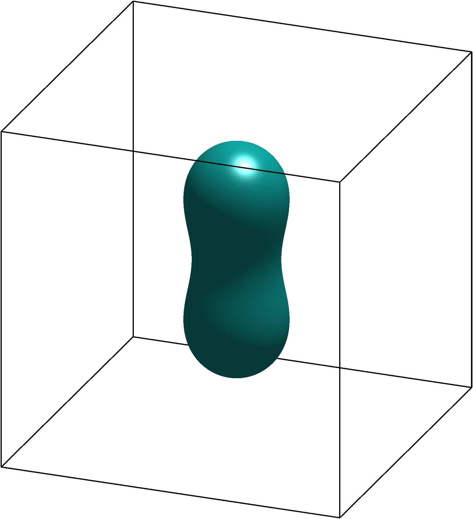
$t_{4}=0.8$	$t_{5}=1.6$	$t_{6}=3.2$	$t_{7}=10$

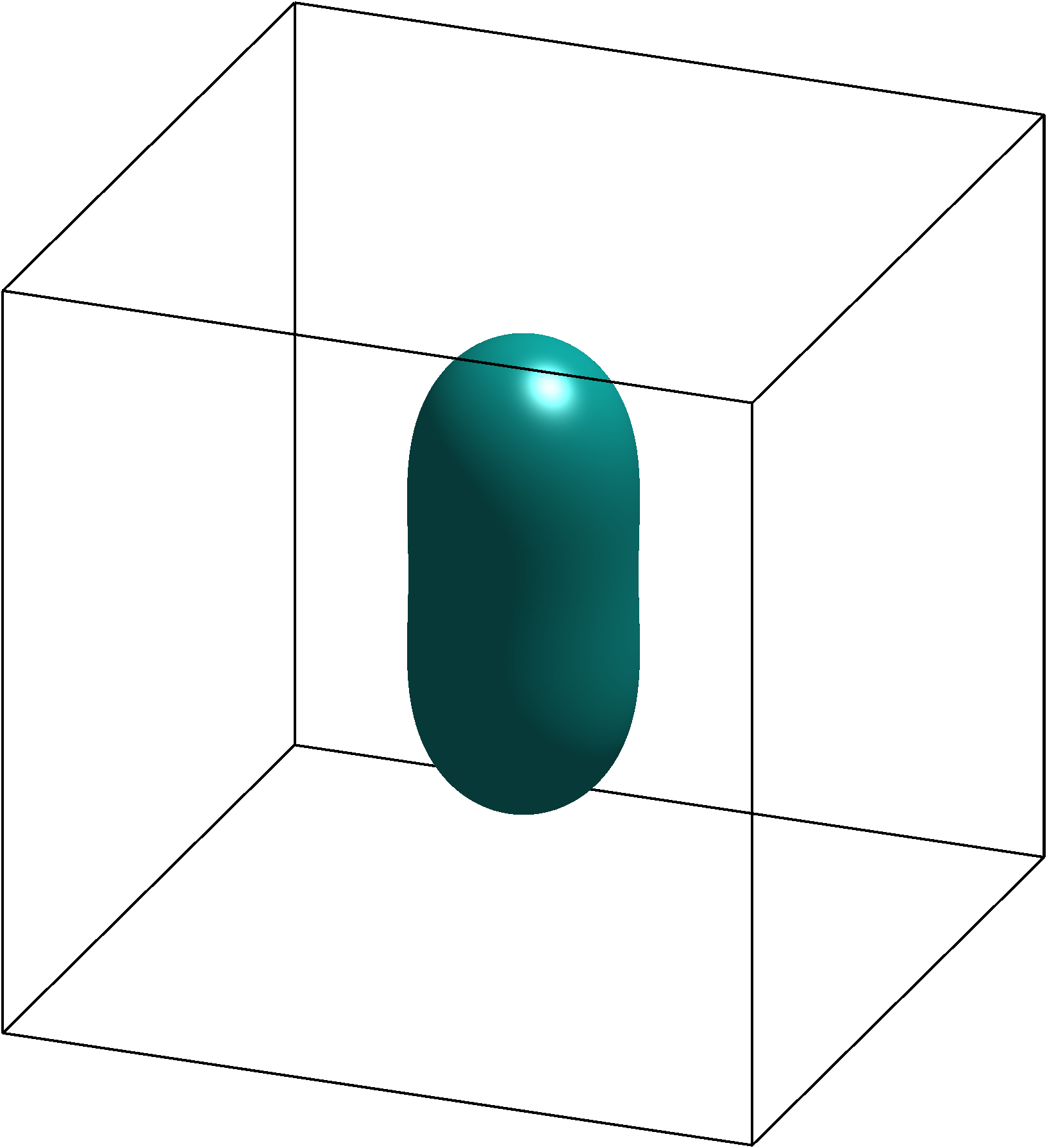
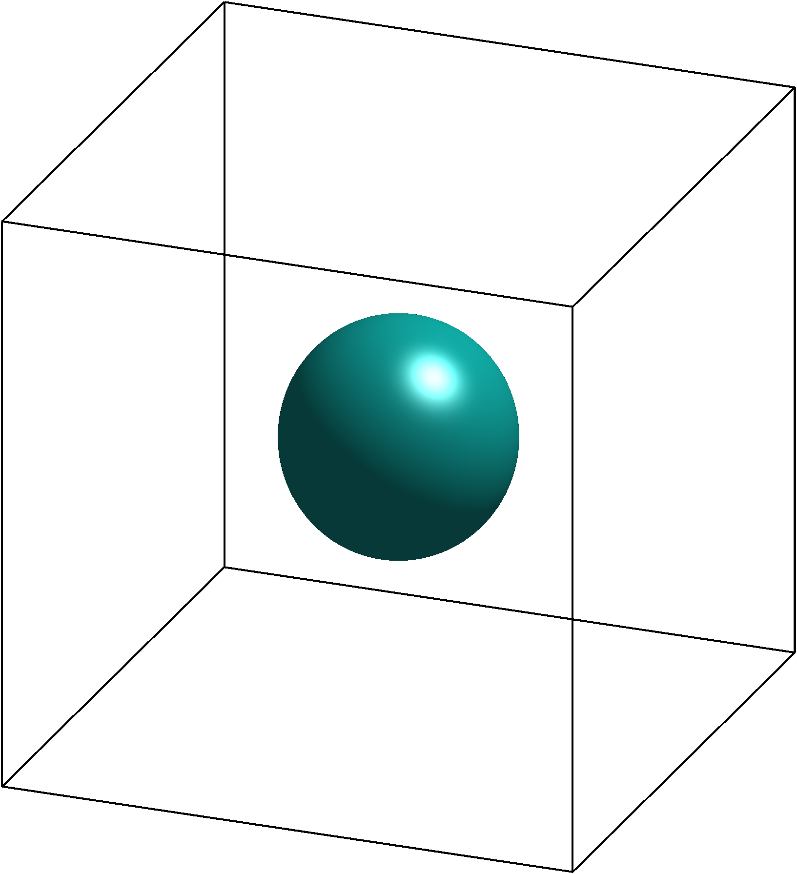
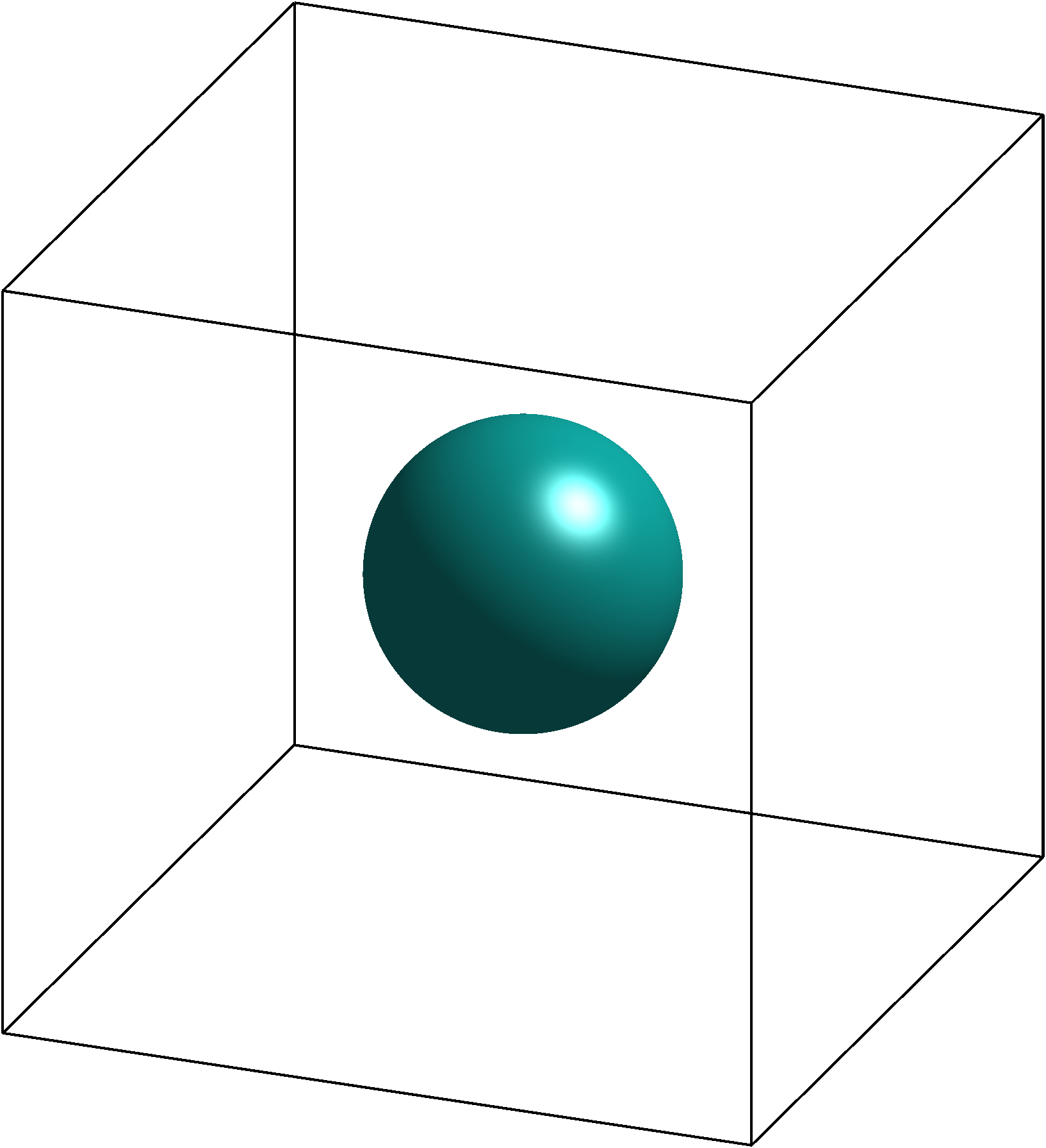
Figure 8: Snapshots of the zero-isocontour of the phase function $\phi$ show the coalescence of two drops at different time instants as indicated.

In Table 11, we enumerate the online computational costs associated with various total DoFs. As explained above, the online computational time at each time step is less than solving two Poisson equations.

Total DoFs	$501^{3}$	$551^{3}$	$601^{3}$	$651^{3}$	$701^{3}$	$751^{3}$
Total time	$8.46$E$2$	$1.29$E$3$	$1.79$E$3$	$2.53$E$3$	$3.10$E$3$	$4.02$E$4$
Time for each time step	$8.46$E-$2$	$1.29$E-$1$	$1.79$E-$1$	$2.53$E-$1$	$3.10$E-$1$	$4.02$E-$1$
Total DoFs	$801^{3}$	$851^{3}$	$901^{3}$	$951^{3}$	$1001^{3}$	$1051^{3}$
Total time	$5.41$E$3$	$6.79$E$3$	$8.84$E$3$	$1.03$E$4$	$1.27$E$4$	-
Time for each time step	$5.41$E-$1$	$6.79$E-$1$	$8.84$E-$1$	$1.03$E$0$	$1.27$E$0$	-

Table 11: Online computational time in seconds for $Q^{5}$ SEM in the BDF2 scheme (24) solving the Cahn–Hilliard equation with 10,000 time steps on Nivida A100. The Total time represents the online computational time for 10,000 time steps, and the Time for each time step is average online computational time per time step.

4 Concluding remarks

In this paper, we have discussed a simple MATLAB 2023 implementation for accelerating high order methods on GPUs. For large enough 3D problems, a speed-up of at least 60 can be achieved on Nvidia A100. In particular, solving a 3D Poisson type equation with one billion DoFs costs only 0.8 second for $Q^{k}$ spectral-element method.

Appendix A MATLAB scripts for a 3D Poisson equation

We provide a demonstration in MATLAB 2023 for $Q^{k}$ spectral-element method solving a Poisson equation in three dimensions, which involves three MATLAB scripts:

1. Poisson3D.m for solving the Poisson equation on either CPU or GPU;

2. SEGenerator1D.m for generating stiffness and mass matrices in spectral element method;

3. LegendreD.m for Legendre and Jocaboi polynomials from [9].

Readers can easily reproduce the results in Section 3.1 and Section 3.2 using these three MATLAB scripts.

Poisson3D.m:

⬇

% Solving the Poisson equation by Q5 SEM with Neumann b.c. gpuDeviceCount('available')<1; Param.device='cpu';

else;Param.device='gpu'; Param.deviceID=1;end % ID=1,2,3,...

Np=5; Param.Np=Np; % polynomial degree Q5

Ncellx=40; Ncelly=40; Ncellz=40; % finite element cell number

% total number of unknowns in each direction

nx=Ncellx*Np+1; ny=Ncelly*Np+1; nz=Ncellz*Np+1;

% the domain is [-Lx, Lx]*[-Ly, Ly]*[-Lz, Lz]

Lx=1; Ly=1; Lz=1; cx=pi; cy=2*pi; cz=3*pi; alpha=1;

Param.Ncellx=Ncellx; Param.Ncelly=Ncelly; Param.Ncellz=Ncellz;

Param.nx = nx; Param.ny = ny; Param.nz = nz;

fprintf('3D Poisson with total DoFs %d by %d by %d \n',nx,ny,nz);

fprintf('Laplacian is Q%d spectral element method \n', Np);

[x,ex,Tx,eigx]=SEGenerator1D('x',Lx,Param);

[y,ey,Ty,eigy]=SEGenerator1D('y',Ly,Param);

[z,ez,Tz,eigz]=SEGenerator1D('z',Lz,Param);

% a smooth solution

u1x=cos(cx*x); u2x=power(1-power(x,2),3);

du2x=30*power(x,4)-36*power(x,2)+6;

u1y=cos(cy*y); u2y=power(1-power(y,2),2);

du2y=4-12*power(y,2);

u1z=cos(cz*z); u2z=power(1-power(z,2),4);

du2z=(8-56*power(z,2)).*power(1-power(z,2),2);

uexact=squeeze(tensorprod(u1x*u1y',u1z)+tensorprod(u2x*u2y',u2z));

f=(cx*cx+cy*cy+cz*cz)*squeeze(tensorprod(u1x*u1y',u1z))+...

squeeze(tensorprod(du2x*u2y',u2z)+tensorprod(u2x*du2y',u2z)+...

tensorprod(u2x*u2y',du2z))+alpha*uexact;

TxInv=pinv(Tx); TyInv=pinv(Ty); TzInv=pinv(Tz);

if strcmp(Param.device,'gpu');Device=gpuDevice(Param.deviceID);

fprintf('GPU computation: starting to load matrices/data \n');

Tx=gpuArray(Tx); Ty=gpuArray(Ty); Tz=gpuArray(Tz);

eigx=gpuArray(eigx);eigy=gpuArray(eigy);eigz=gpuArray(eigz);

ex=gpuArray(ex); ey=gpuArray(ey); ez=gpuArray(ez); f=gpuArray(f);

TxInv=gpuArray(TxInv);TyInv=gpuArray(TyInv);TzInv=gpuArray(TzInv);

end

Lambda3D=squeeze(tensorprod(eigx,ey*ez')+tensorprod(ex,eigy*ez')...

+tensorprod(ex,ey*eigz'));

if strcmp(Param.device,'gpu'); wait(Device);

fprintf('GPU loading finished and computing started \n');

end

tic; % online computation

u = tensorprod(f,TzInv',3,1);

u = pagemtimes(u,TyInv');

u = squeeze(tensorprod(TxInv,u,2,1));

u = u./(Lambda3D + alpha);

u = tensorprod(u,Tz',3,1);

u = pagemtimes(u,Ty');

u = squeeze(tensorprod(Tx,u,2,1));

if strcmp(Param.device,'gpu');wait(Device);end;time=toc;err=u-uexact;

fprintf('The ell infinity norm error is %d \n',norm(err(:),inf));

if strcmp(Param.device,'gpu')

fprintf('The online GPU computation time is %d \n', time);

else

fprintf('The online CPU computation time is %d \n', time);

end

SEGenerator1D.m:

⬇

ction [varargout] = SEGenerator1D(direction,L,Param)

% generate 1D spectral element with Neumann B.C.

switch direction

case 'x'

N=Param.Np; Ncell=Param.Ncellx; n=Param.nx;

case 'y'

N=Param.Np; Ncell=Param.Ncelly; n=Param.ny;

case 'z'

N=Param.Np; Ncell=Param.Ncellz; n=Param.nz;

end

% generate the mesh with Ncell intervals with domain [Left, Right]

[D,r,w] = LegendreD(N); Left = -L; Right = L;

Length = Right - Left; dx = Length/Ncell;

for j = 1:Ncell

cellLeft = Left+dx*(j-1);

localPoints = cellLeft+dx/2+r*dx/2;

if (j==1)

x = localPoints;

else

x = [x;localPoints(2:end)];

end

end

SLocal = D'*diag(w)*D; % local stiffness matrix for each element

S=[]; M=[];

for j = 1:Ncell % global stiffness and lumped mass matrices

S = blkdiag(SLocal,S); M = blkdiag(diag(w),M);

end

% Next step: "glue" the cells

Np = N+1; % number of points in each cell

Glue = sparse(zeros(Ncell*Np-Ncell+1, Ncell*Np));

for j = 1:Ncell

rowStart=(j-1)*Np+2-j; rowEnd=rowStart+Np-1;

colStart=(j-1)*Np+1; colEnd=colStart+Np-1;

Glue(rowStart:rowEnd,colStart:colEnd)=speye(Np);

end

S=Glue*S*Glue'; M=Glue*M*Glue'; H=diag(1./diag(M))*S;

ex=ones(n,1); MHalfInv=diag(1./sqrt(diag(M)));

S1=MHalfInv*S*MHalfInv; S1=(S1+S1')/2;

[U,d]=eig(S1,'vector'); [lambda,indexSort]=sort(d);

T=U(:,indexSort); h=dx/2; lambda=lambda/(h*h);

S1=sparse(S1/(h*h)); M=sparse(M);

% after this step, T is the eigenvector of H

T = MHalfInv*T; H=full(H/(h*h)); S=S/h; M=full(M*h);

varargout{1}=x; varargout{2}=ex; varargout{3}=T; varargout{4}=lambda;

end

LegendreD.m:

⬇

ction [D,r,w] = LegendreD(N)

Np = N+1; r = JacobiGL(0,0,N);

w = (2*N+1)/(N*N+N)./power(JacobiP(r,0,0,N),2);

Distance = r*ones(1,N+1)-ones(N+1,1)*r'+eye(N+1);

omega = prod(Distance,2);

D = diag(omega)*(1./Distance)*diag(1./omega);

D(1:Np+1:end) = 0; D(1:Np+1:end) = -sum(D,2);

end

function [x] = JacobiGL(alpha,beta,N)

x = zeros(N+1,1);

if (N==1); x(1)=-1.0; x(2)=1.0; return; end

[xint,temp] = JacobiGQ(alpha+1,beta+1,N-2);

x = [-1, xint', 1]'; return;

end

function [x,w] = JacobiGQ(alpha,beta,N)

if (N==0)

x(1) = -(alpha-beta)/(alpha+beta+2); w(1) = 2; return;

end

h1 = 2*(0:N)+alpha+beta;

J = diag(-1/2*(alpha*alpha-beta*beta)./(h1+2)./h1) + ...

diag(2./(h1(1:N)+2).*sqrt((1:N).*((1:N)+alpha+beta).*...

((1:N)+alpha).*((1:N)+beta)./(h1(1:N)+1)./(h1(1:N)+3)),1);

if (alpha+beta<10*eps); J(1,1)=0.0; end

J = J + J'; [V,D] = eig(J); x = diag(D);

w = power(V(1,:)',2)*power(2,alpha+beta+1)/(alpha+beta+1)*...

gamma(alpha+1)*gamma(beta+1)/gamma(alpha+beta+1);

end

function [P] = JacobiP(x,alpha,beta,N)

xp = x; dims = size(xp);

if (dims(2)==1); xp = xp'; end

PL = zeros(N+1,length(xp));

gamma0 = power(2,alpha+beta+1)/(alpha+beta+1)*gamma(alpha+1)*...

gamma(beta+1)/gamma(alpha+beta+1);

PL(1,:) = 1.0/sqrt(gamma0);

if (N==0); P = PL'; return; end

gamma1 = (alpha+1)*(beta+1)/(alpha+beta+3)*gamma0;

PL(2,:) = ((alpha+beta+2)*xp/2 + (alpha-beta)/2)/sqrt(gamma1);

if (N==1); P = PL(N+1,:)'; return; end

aold = 2/(2+alpha+beta)*sqrt((alpha+1)*(beta+1)/(alpha+beta+3));

for i = 1:N-1

h1 = 2*i+alpha+beta;

anew = 2/(h1+2)*sqrt( (i+1)*(i+1+alpha+beta)*(i+1+alpha)*...

(i+1+beta)/(h1+1)/(h1+3));

bnew = - (alpha*alpha-beta*beta)/h1/(h1+2);

PL(i+2,:) = 1/anew*( -aold*PL(i,:) + (xp-bnew).*PL(i+1,:));

aold = anew;

end

P = PL(N+1,:)';

end

References

- [1] John W Cahn and John E Hilliard. Free energy of a nonuniform system. i. interfacial free energy. The Journal of chemical physics, 28(2):258–267, 1958.
- [2] Feng Chen and Jie Shen. Efficient spectral-Galerkin methods for systems of coupled second-order equations and their applications. Journal of Computational Physics, 231(15):5016–5028, 2012.
- [3] Feng Chen and Jie Shen. A GPU parallelized spectral method for elliptic equations in rectangular domains. Journal of Computational Physics, 250:555–564, 2013.
- [4] Sheng Chen and Jie Shen. An efficient and accurate numerical method for the spectral fractional Laplacian equation. Journal of Scientific Computing, 82(1):17, 2020.
- [5] Ziang Chen, Jianfeng Lu, Yulong Lu, and Xiangxiong Zhang. On the convergence of Sobolev gradient flow for the Gross-Pitaevskii eigenvalue problem. arXiv preprint arXiv:2301.09818, 2023.
- [6] Qiang Du, Lili Ju, Xiao Li, and Zhonghua Qiao. Maximum principle preserving exponential time differencing schemes for the nonlocal Allen–Cahn equation. SIAM Journal on numerical analysis, 57(2):875–898, 2019.
- [7] Jean-Luc Guermond, Peter Minev, and Jie Shen. An overview of projection methods for incompressible flows. Computer methods in applied mechanics and engineering, 195(44-47):6011–6045, 2006.
- [8] Dale B Haidvogel and Thomas Zang. The accurate solution of Poisson’s equation by expansion in Chebyshev polynomials. Journal of Computational Physics, 30(2):167–180, 1979.
- [9] Jan S Hesthaven and Tim Warburton. Nodal discontinuous Galerkin methods: algorithms, analysis, and applications. Springer Science & Business Media, 2007.
- [10] Jingwei Hu and Xiangxiong Zhang. Positivity-preserving and energy-dissipative finite difference schemes for the Fokker–Planck and Keller–Segel equations. IMA Journal of Numerical Analysis, 43(3):1450–1484, 2023.
- [11] A. Klöckner, T. Warburton, J. Bridge, and J.S. Hesthaven. Nodal discontinuous Galerkin methods on graphics processors. Journal of Computational Physics, 228(21):7863–7882, 2009.
- [12] Yuen-Yick Kwan and Jie Shen. An efficient direct parallel spectral-element solver for separable elliptic problems. Journal of Computational Physics, 225(2):1721–1735, 2007.
- [13] Hao Li, Daniel Appelö, and Xiangxiong Zhang. Accuracy of Spectral Element Method for Wave, Parabolic, and Schrödinger Equations. SIAM Journal on Numerical Analysis, 60(1):339–363, 2022.
- [14] Hao Li and Xiangxiong Zhang. Superconvergence of high order finite difference schemes based on variational formulation for elliptic equations. Journal of Scientific Computing, 82(2):36, 2020.
- [15] Re Lynch, John R Rice, and Donald H Thomas. Tensor product analysis of partial difference equations. Bull. Amer. Math. Soc., 70, 1964.
- [16] Yvon Maday and Einar M Rønquist. Optimal error analysis of spectral methods with emphasis on non-constant coefficients and deformed geometries. Computer Methods in Applied Mechanics and Engineering, 80(1-3):91–115, 1990.
- [17] Anthony T Patera. Fast direct poisson solvers for high-order finite element discretizations in rectangularly decomposable domains. Journal of Computational Physics, 65(2):474–480, 1986.
- [18] Jie Shen. Efficient spectral-Galerkin method I. Direct solvers of second-and fourth-order equations using Legendre polynomials. SIAM Journal on Scientific Computing, 15(6):1489–1505, 1994.
- [19] Jie Shen, Jie Xu, and Jiang Yang. A new class of efficient and robust energy stable schemes for gradient flows. SIAM Review, 61(3):474–506, 2019.
- [20] Jie Shen and Xiangxiong Zhang. Discrete maximum principle of a high order finite difference scheme for a generalized Allen–Cahn equation. Communications in Mathematical Sciences, 20(5):1409–1436, 2022.