A Prefrontal Cortex-inspired Architecture for Planning in Large Language Models

Abstract

Large language models (LLMs) demonstrate impressive performance on a wide variety of tasks, but they often struggle with tasks that require multi-step reasoning or goal-directed planning. To address this, we take inspiration from the human brain, in which planning is accomplished via the recurrent interaction of specialized modules in the prefrontal cortex (PFC). These modules perform functions such as conflict monitoring, state prediction, state evaluation, task decomposition, and task coordination. We find that LLMs are sometimes capable of carrying out these functions in isolation, but struggle to autonomously coordinate them in the service of a goal. Therefore, we propose a black box architecture with multiple LLM-based (GPT-4) modules. The architecture improves planning through the interaction of specialized PFC-inspired modules that break down a larger problem into multiple brief automated calls to the LLM. We evaluate the combined architecture on two challenging planning tasks – graph traversal and Tower of Hanoi – finding that it yields significant improvements over standard LLM methods (e.g., zero-shot prompting or in-context learning). These results demonstrate the benefit of utilizing knowledge from cognitive neuroscience to improve planning in LLMs.

1 Introduction

Large Language Models (LLMs) (Devlin et al., 2090; Brown et al., 2020) have recently emerged as highly capable generalist systems with a surprising range of emergent capacities (Srivastava et al., 2022; Wei et al., 2022a; Webb et al., 2023). They have also sparked broad controversy, with some suggesting that they are approaching general intelligence (Bubeck et al., 2023), and others noting a number of significant deficiencies (Mahowald et al., 2023). A particularly notable shortcoming is their poor ability to plan or perform faithful multi-step reasoning (Valmeekam et al., 2023; Dziri et al., 2023). Recent work (Momennejad et al., 2023) has evaluated the extent to which LLMs might possess an emergent capacity for planning and exploiting cognitive maps, the relational structures that humans and other animals utilize to perform planning (Tolman, 1948; Tavares et al., 2015; Behrens et al., 2018). This work found that a variety of LLMs, ranging from small, open-source models (e.g., LLaMA-13B and Alpaca-7B) to large, state-of-the-art models (e.g., GPT-4), displayed systematic shortcomings in planning tasks that suggested an inability to reason about cognitive maps. Common failure modes included a tendency to ‘hallucinate’ (e.g., to imagine non-existent paths), and to fall into loops. This work raises the question of how LLMs might be improved so as to enable a capacity for planning.

In the present work, we take a step toward improving planning in LLMs, by taking inspiration from the planning mechanisms employed by the human brain. Planning is generally thought to depend on the prefrontal cortex (PFC) (Owen, 1997; Russin et al., 2020; Brunec & Momennejad, 2022; Momennejad et al., 2018; Momennejad, 2020; Mattar & Lengyel, 2022), a region in the frontal lobe that is broadly involved in executive function, decision-making, and reasoning (Miller & Cohen, 2001). Research in cognitive neuroscience has revealed the presence of several subregions or modules within the PFC that appear to be specialized to perform certain functions. These include functions such as conflict monitoring (Botvinick et al., 1999); state prediction and state evaluation (Wallis, 2007; Schuck et al., 2016); and task decomposition and task coordination  (Ramnani & Owen, 2004; Momennejad & Haynes, 2012; 2013). Human planning then emerges through the coordinated and recurrent interactions among these specialized PFC modules, rather than through the activity of a single, monolithic system.

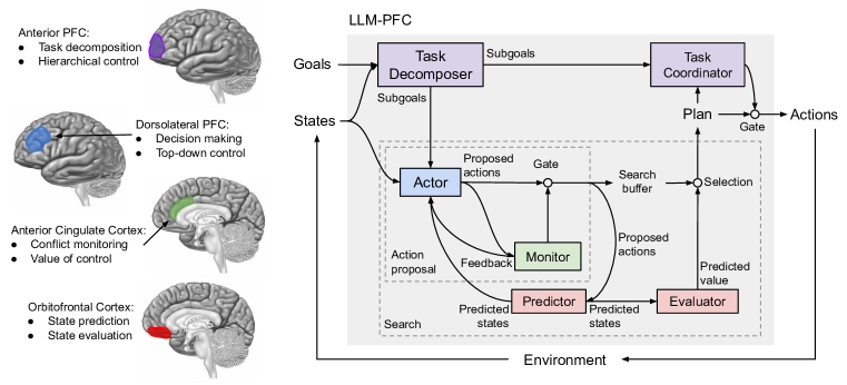
Figure 1: LLM-PFC architecture. The agent receives states from the environment and high-level goals. These are processed by a set of specialized LLM modules. The $\operatorname{TaskDecomposer}$ receives high-level goals and generates a series of subgoals. The $\operatorname{Actor}$ generates proposed actions given a state and a subgoal. The $\operatorname{Monitor}$ gates these proposed actions based on whether they violate certain constraints (e.g., task rules) and provides feedback to the $\operatorname{Actor}$. The $\operatorname{Predictor}$ predicts the next state given the current state and a proposed action. The $\operatorname{Evaluator}$ is used to estimate the value of a predicted state. The $\operatorname{Predictor}$ and $\operatorname{Evaluator}$ are used together to perform tree search. The $\operatorname{TaskCoordinator}$ determines when each subgoal has been achieved, and when the final goal has been achieved, at which point the plan is emitted to the environment as a series of actions. These modules are inspired by the specific PFC subregions depicted on the left.

An interesting observation is that LLMs often seem to display some of these capacities when probed in isolation, even though they are unable to reliably integrate and deploy these capacities in the service of a goal. For instance,  Momennejad et al. (2023) noted that LLMs often attempt to traverse invalid or hallucinated paths in planning problems (e.g., to move between rooms that are not connected), even though they can correctly identify these paths as invalid when probed separately. This suggests the possibility of a PFC-inspired approach, in which planning is carried out through the coordinated activity of multiple LLM modules, each of which is specialized to perform a distinct process.

With this goal in mind, we propose LLM-PFC (Figure 1), an architecture composed of modules that are specialized to perform specific PFC-inspired functions. Each module consists of an LLM instance (GPT-4), constructed through a combination of prompting and few-shot in-context learning. We specifically propose modules that perform error monitoring, action proposal, state prediction, state evaluation, task decomposition, and task coordination. It is suggested that the coordinated activity of multiple PFC subregions performs tree search during planning (Owen, 1997; Daw et al., 2005; Wunderlich et al., 2012; Doll et al., 2015). Thus, our approach combines action proposal, state prediction, and state evaluation to perform tree search.

We evaluate LLM-PFC on two challenging planning tasks. First, we performed controlled experiments on a set of graph traversal tasks using the CogEval protocol  (Momennejad et al., 2023). These tasks require navigation in novel environments based on natural language descriptions, and have been shown to be extremely challenging for LLMs, including GPT-4. Second, we investigate Tower of Hanoi (ToH), a classic problem solving task that requires multi-step planning (Simon, 1975), and for which performance is known to be heavily dependent on PFC function (Goel & Grafman, 1995; Fincham et al., 2002). We find that our approach significantly improves LLM performance on these planning tasks, yielding nearly perfect performance on the graph traversal tasks, and a nearly seven-fold improvement over zero-shot performance on Tower of Hanoi (74% vs. 11% accuracy). Ablation experiments further indicate that each of the individual modules plays an important role in the overall architecture’s performance. Taken together, these results indicate the potential of a PFC-inspired approach to improve the reasoning and planning capabilities of LLMs.

2 Approach

The LLM-PFC architecture is constructed from a set of a specialized LLM modules, each of which performs a specific PFC-inspired function. In the following sections, we first describe the functions performed by each module, and then describe how they interact to generate a plan.

2.1 Modules

LLM-PFC contains the following specialized modules, each constructed from a separate LLM instance through a combination of prompting and few-shot ($\leq 3$ examples) in-context learning (described in greater detail in section A.2):

$\bullet$ $\operatorname{\mathbf{TaskDecomposer}}$. The $\operatorname{TaskDecomposer}$ receives the current state $\displaystyle x$ and a goal $\displaystyle y$ and generates a set of subgoals $\displaystyle Z$ that will allow the agent to gradually work toward its final goal. This module is inspired by the anterior PFC (aPFC), which is known to play a key role in task decomposition through the generation and maintenance of subgoals (Ramnani & Owen, 2004). In the present work, the $\operatorname{TaskDecomposer}$ is only utilized to generate a single intermediate goal, though in future work we envision that it will be useful to generate a series of multiple subgoals.

$\bullet$ $\operatorname{\mathbf{Actor}}$. The $\operatorname{Actor}$ receives the current state $\displaystyle x$ and a subgoal $\displaystyle z$ and proposes $\displaystyle B$ potential actions $\displaystyle A=a_{b=1}\dots a_{b=B}$. The $\operatorname{Actor}$ can also receive feedback $\displaystyle\epsilon$ from the $\operatorname{Monitor}$ about its proposed actions. This module can be viewed as being analogous to the dorsolateral PFC (dlPFC) which plays a role in decision making through top-down control and guidance of lower-order premotor and motor regions (Miller & Cohen, 2001).

$\bullet$ $\operatorname{\mathbf{Monitor}}$. The $\operatorname{Monitor}$ assesses the actions proposed by the $\operatorname{Actor}$ to determine whether they are valid (e.g., whether they violate the rules of a task). It emits an assessment of validity $\displaystyle\sigma$, and also feedback $\displaystyle\epsilon$ in the event the action is deemed invalid. This module is inspired by the Anterior Cingulate Cortex (ACC), which is known to play a role in conflict monitoring (Botvinick et al., 1999), i.e., detecting errors or instances of ambiguity.

$\bullet$ $\operatorname{\mathbf{Predictor}}$. The $\operatorname{Predictor}$ receives the current state $\displaystyle x$ and a proposed action $\displaystyle a$ and predicts the resulting next state $\displaystyle\tilde{x}$. The $\operatorname{Predictor}$ is inspired by the Orbitofrontal cortex (OFC), which plays a role in estimating and predicting task states. In particular, it has been proposed that the OFC plays a key role in encoding cognitive maps: representations of task-relevant states and their relationships to one another (Schuck et al., 2016).

$\bullet$ $\operatorname{\mathbf{Evaluator}}$. The $\operatorname{Evaluator}$ receives a next-state prediction $\displaystyle\tilde{x}$ and produces an estimate of its value $\displaystyle v$ in the context of goal $\displaystyle y$. This is accomplished by prompting the $\operatorname{Evaluator}$ (and demonstrating via a few in-context examples) to estimate the minimum number of steps required to reach the goal (or subgoal) from the current state. The $\operatorname{Evaluator}$ is also inspired by the OFC which, in addition to predicting task states, plays a key role in estimating the motivational value of those states Wallis (2007).

$\bullet$ $\operatorname{\mathbf{TaskCoordinator}}$. The $\operatorname{TaskCoordinator}$ receives the current state $\displaystyle x$ and a subgoal $\displaystyle z$ and emits an assessment $\displaystyle\Omega$ of whether the subgoal has been achieved. When the $\operatorname{TaskCoordinator}$ determines that all subgoals (including the final goal) have been achieved, the plan is emitted to the environment as a series of actions. This module is also inspired by the aPFC, which is thought to both identify subgoals and coordinate their sequential execution (Ramnani & Owen, 2004).

2.2 Action proposal loop

The $\operatorname{Actor}$ and $\operatorname{Monitor}$ interact via the $\operatorname{ProposeAction}$ function (Algorithm 1). The $\operatorname{Actor}$ proposes actions which are then gated by the $\operatorname{Monitor}$. If the $\operatorname{Monitor}$ determines that the actions are invalid (e.g., they violate the rules of a task), feedback is provided to the $\operatorname{Actor}$, which then proposes an alternative action. In the brain, a similar process is carried out by interactions between the ACC and dorsolateral PFC (dlPFC). The ACC is thought to recruit the dlPFC under conditions of conflict (e.g., errors or ambiguity), which then acts to resolve the conflict through top-down projections to lower-order control structures (e.g., premotor and motor cortices) (Miller & Cohen, 2001; Shenhav et al., 2013).

Function $\operatorname{ProposeAction}$($\displaystyle x,y,B$):

       $\displaystyle\sigma\leftarrow$ false // Initialize validity

       $\displaystyle E\leftarrow$ $\{\}$ // Initialize feedback

       while $\displaystyle\sigma$ is false do

             $\displaystyle A\leftarrow\operatorname{Actor}(x,y,E,B)$ // Sample B actions

             $\displaystyle\sigma,\epsilon\leftarrow\operatorname{Monitor}(x,A)$ // Determine validity and provide feedback

             $\displaystyle E\leftarrow E\cup\{\epsilon\}$ // Accumulate feedback

            

       end while

      

return $\displaystyle A$

Algorithm 1 Action proposal loop. $\operatorname{ProposeAction}$ takes a state $\displaystyle x$ and a goal $\displaystyle y$ and generates $\displaystyle B$ potential actions $\displaystyle A=a_{b=1}\dots a_{b=B}$. This is implemented via a loop, in which the $\operatorname{Actor}$ first proposes potential actions, and the $\operatorname{Monitor}$ then assesses those actions according to certain constraints (e.g., task rules), providing feedback if any of the actions are deemed to be invalid. This continues until the proposed actions are considered valid. See Sections A.2.2 and A.2.3 for more details.

2.3 Search loop

$\operatorname{ProposeAction}$ is further embedded in a $\operatorname{Search}$ loop (Algorithm 2). The actions emitted by $\operatorname{ProposeAction}$ are passed to the $\operatorname{Predictor}$, which predicts the states that will result from these actions. A limited tree search is then performed, starting from the current state, and then exploring $\displaystyle B$ branches recursively to a depth of $\displaystyle L$ layers. Values are assigned to the terminal states of this search by the $\operatorname{Evaluator}$, and the action leading to the most valuable predicted state is selected. This approach mirrors that of the human brain, in which search is thought to be carried out through the coordinated activity of multiple regions within the PFC, including dlPFC, ACC, and OFC (Owen, 1997; Mattar & Lengyel, 2022).

Function $\operatorname{Search}$($\displaystyle l,L,B,x,y$):

       $\displaystyle V_{l}\leftarrow\{\}$ // Initialize value record

       $\displaystyle\tilde{X}_{l}\leftarrow\{\}$ // Initialize next-state record

       $\displaystyle A_{l}\leftarrow\operatorname{ProposeAction}(x,y,B)$ // Propose B actions

       for $b$ in $1\ldots B$ do

             $\displaystyle\tilde{x}_{lb}\leftarrow\operatorname{Predictor}(x,A_{lb})$ // Predict next state

             $\displaystyle\tilde{X}_{l}\leftarrow\tilde{X}_{l}\cup\{\tilde{x}_{lb}\}$ // Update next-state record

             $\displaystyle\Omega\leftarrow\operatorname{TaskCoordinator}(\tilde{x}_{lb},y)$ // Terminate search if goal achieved

             if $l<L$ and $\displaystyle\Omega$ is false then

                   $\displaystyle a_{l+1},\tilde{x}_{l+1},v_{l+1}\leftarrow\operatorname{Search}(l+1,L,B,\tilde{x}_{lb},y)$ // Advance search depth

                   $\displaystyle V_{l}\leftarrow V_{l}\cup\{v_{l+1}\}$ // Update value record

                  

            else

                   $\displaystyle v_{lb}\leftarrow\operatorname{Evaluator}(\tilde{x}_{lb},y)$ // Evaluate predicted state

                   $\displaystyle V_{l}\leftarrow V_{l}\cup\{v_{lb}\}$ // Update value record

                  

             end if

            

       end for

      $\displaystyle v_{l}\leftarrow\operatorname{max}(V_{l})$ // Maximum value (randomly sample if equal value)

       $\displaystyle a_{l}\leftarrow A_{l\operatorname{argmax}(V_{l})}$ // Select action

       $\displaystyle\tilde{x}_{l}\leftarrow\tilde{X}_{l{\operatorname{argmax}(V_{l})}}$ // Predicted next-state

      

return $\displaystyle a_{l},\tilde{x}_{l},v_{l}$

Algorithm 2 Search loop. Tree search with a depth of $\displaystyle L$ layers, with $\displaystyle B$ branches at each layer $\displaystyle l$. For each branch, a proposed action is sampled, and the $\operatorname{Predictor}$ predicts the next state $\displaystyle\tilde{x}$. This process continues resursively until the terminal layer $\displaystyle L$, at which point the value $\displaystyle v_{l=L}$ of the terminal states is estimated by the $\operatorname{Evaluator}$. The values are backpropogated to their parent states in the first layer, and the action that leads to the most valuable state is selected. In our implementation, we accelerate this process by caching the actions and predicted states from deeper search layers and then reusing them in subsequent searches. We also employ the $\operatorname{TaskCoordinator}$ to prematurely terminate search if the goal state is achieved.

Function $\operatorname{LLM-PFC}$($\displaystyle x,y,T,L,B$):

       $\displaystyle P\leftarrow[]$ // Initialize plan

       $\displaystyle Z\leftarrow\operatorname{TaskDecomposer}(x,y)$ // Generate subgoals

       for $g$ in $1\ldots\operatorname{length}(Z)+1$ do

             if $g\leq\operatorname{length}(Z)$ then

                   $\displaystyle z\leftarrow Z_{g}$ // Update current subgoal

                  

            else

                   $\displaystyle z\leftarrow y$ // Final goal

                  

             end if

            $\displaystyle\Omega\leftarrow\operatorname{TaskCoordinator}(x,z)$ // Initialize subgoal assessment

             while $\displaystyle\Omega$ is false and $\displaystyle\operatorname{length}(P)<T$ do

                   $\displaystyle a,x,v\leftarrow\operatorname{Search}(l=1,L,B,x,z)$ // Perform search

                   $\displaystyle P\leftarrow[P,a]$ // Update plan

                   $\displaystyle\Omega\leftarrow\operatorname{TaskCoordinator}(x,z)$ // Determine if subgoal is achieved

                  

             end while

            

       end for

      

return $\displaystyle P$

Algorithm 3 LLM-PFC. $\operatorname{LLM-PFC}$ takes a state $\displaystyle x$ and a goal $\displaystyle y$ and generates a plan $\displaystyle P$, a series of actions with a maximum length of $\displaystyle T$. The $\operatorname{TaskDecomposer}$ first generates a set of subgoals $\displaystyle Z$. The agent then pursues each individual subgoal $\displaystyle z$ in sequence, followed by the final goal $\displaystyle y$. At each time step, $\operatorname{Search}$ is called to generate an action and a predicted next-state. Actions are added to the plan until the $\operatorname{TaskCoordinator}$ determines that the goal has been achieved, or the plan reaches the maximum length $\displaystyle T$.

2.4 Plan generation

Algorithm 3 describes the complete LLM-PFC algorithm. To generate a plan, a set of subgoals is first generated by the $\operatorname{TaskDecomposer}$ based on the final goal and current state. These subgoals are then pursued one at a time, utilizing the $\operatorname{Search}$ loop to generate actions until the $\operatorname{TaskCoordinator}$ determines that the subgoal has been achieved. The actions are accumulated in a plan buffer $\displaystyle P$ until either the $\operatorname{TaskCoordinator}$ determines that the final goal has been reached, or the maximum allowable number of actions $\displaystyle T$ are accumulated. This approach is inspired by the role that aPFC plays in task decomposition. This involves the decomposition of tasks into smaller, more manageable tasks, and the coordinated sequential execution of these component tasks (Ramnani & Owen, 2004).

3 Experiments

3.1 Tasks

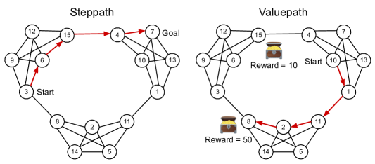
Figure 2: Graph Traversal. We investigated two graph traversal tasks utilizing a challenging graph with community structure. Steppath: Find shortest path between two nodes, e.g. node 3 and node 7. Valuepath: Find shortest path from starting location (e.g., node 10) to location with maximum reward (node 8 in depicted example).

Graph Traversal. We performed controlled experiments on two multi-step planning tasks based on graph traversal using the CogEval protocol (Momennejad et al., 2023). Natural language descriptions of a graph are provided with each node assigned to a room (e.g., ‘room 4 is connected to room 7’). We focused on a particular type of graph (Figure 2) with community structure (Schapiro et al., 2013) previously found to be challenging for a wide variety of LLMs. The first task, Valuepath, involves finding the shortest path from a given room that results in the largest reward possible. A smaller reward and a larger reward are located at two different positions in the graph. We fixed the two reward locations, and created 13 problems based on different starting locations. The second task, Steppath, involves finding the shortest path between a pair of nodes. We evaluated problems with an optimal shortest path of 2, 3, or 4 steps. We generated 20 problems for each of these conditions by sampling different starting and target locations.

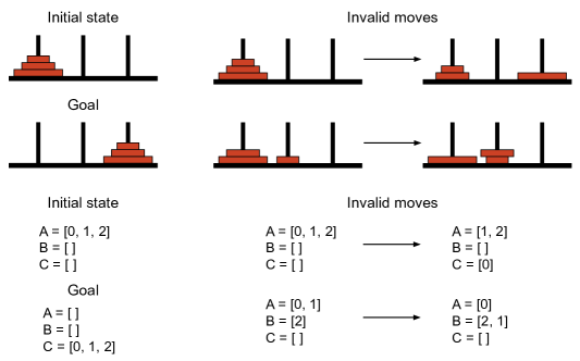
Figure 3: Tower of Hanoi. Top: Depiction of the Tower of Hanoi (ToH) puzzle. Disks are stacked in order of decreasing size on the leftmost peg. The goal is to move these disks so that they are stacked in order of decreasing size on the rightmost peg. Only the disk on the top of the stack may be moved, and a disk can only be placed on top of larger disks (or on an empty peg). The version shown involves three disks, but more disks can be used (making the task significantly more difficult). Bottom: Modified text-based version of ToH. Three lists are presented, labelled A, B and C. A set of integers is distributed amongst these lists. The goal is to move the numbers so that they are arranged in ascending order in list C. Only the number at the end of the list may be moved, and a number can only be placed in front of a smaller number. Multiple problem instances were created by varying the initial state.

Tower of Hanoi. We also investigated a classic multi-step planning task called the Tower of Hanoi (ToH) (Figure 3). In the original formulation, there are three pegs and a set of disks of different sizes. The disks are stacked in order of decreasing size on the leftmost peg. The goal is to move all disks to the rightmost peg, such that the disks are stacked in order of decreasing size. There are a couple of rules that determine which moves are considered valid. First, a disk can only be moved if it is at the top of its stack. Second, a disk can only be moved to the top of another stack if it is smaller than the disks in that stack (or if the peg is empty). More complex versions of the task can be created by using a larger number of disks.

We designed an alternative formulation of this task in which the inputs are text-based rather than visual. In this alternative formulation, three lists (A, B, and C) are used instead of the three pegs, and a set of numbers (0, 1, 2, and so on) is used instead of disks of different sizes. The goal is to move all numbers so that they are arranged in ascending order in list C. The rules are isomorphic to ToH. First, a number can only be moved if it is at the end of a list. Second, a number can only be moved to the end of a new list if it is larger than all the numbers in that list. Note that although this novel formulation is isomorphic to ToH (and equally complex), it does not share any surface features with the original ToH puzzle (disks, pegs, etc.), and thus GPT-4 cannot rely on exposure to descriptions of ToH in its training data to solve the problem. We created multiple problem instances by varying the initial state (the initial positions of the numbers). This resulted in 26 three-disk problems and 80 four-disk problems.

3.2 Baselines

We compared our model to two baseline methods. The first method involved asking GPT-4 (zero-shot) to provide the solution step by step. For the second method, in-context learning (ICL), we provided GPT-4 with a few in-context examples of a complete solution. We provided two examples for ToH and Valuepath, and 3 examples (one each for 2, 3, and 4 steps) for Steppath.

3.3 Experiment Details

We implemented each of the modules using a separate GPT-4 (32K context, ‘2023-03-15-preview’ model index, Microsoft Azure openAI service) instance through a combination of prompting and few-shot in-context examples. We set Top-p to 0 and temperature to 0, except for the $\operatorname{Actor}$ (as detailed in section A.2.2). The $\operatorname{Search}$ loop explored $B=2$ branches recursively for a depth $L=2$.

For ToH, we used two randomly selected in-context examples of three-disk problems, and a description of the problem in the prompts for all the modules. For the graph traversal tasks, we used two in-context examples for all modules, except for the $\operatorname{Actor}$ and $\operatorname{Evaluator}$ in the Steppath task, where we used three in-context examples, one each for 2-, 3-, and 4-step paths. The prompt also described the specific task that was to be performed by each module (e.g., monitoring, task decomposition). For more details about the prompts and specific procedures used for each module, see Section A.2.

For three-disk problems, we allowed a maximum of $\displaystyle T=10$ actions per problem, and evaluated on 24 out of 26 possible problems (leaving out the two problems that were used as in-context examples for the $\operatorname{Actor}$). We also evaluated on four-disk problems, for which we allowed a maximum of $\displaystyle T=20$ actions per problem. The same three-disk problems were used as in-context examples, meaning that the four-disk problems tested for out-of-distribution (OOD) generalization. For the graph traversal tasks, we allowed a maximum of $\displaystyle T=6$ actions per problem.

We didn’t use a separate $\operatorname{Predictor}$ for the graph traversal tasks, since the action proposed by the $\operatorname{Actor}$ gives the next state. We also did not include the $\operatorname{TaskDecomposer}$ for these tasks, and did not use the $\operatorname{Search}$ loop for the Steppath task, as the model’s performance was already at ceiling without the use of these components.

4 Results

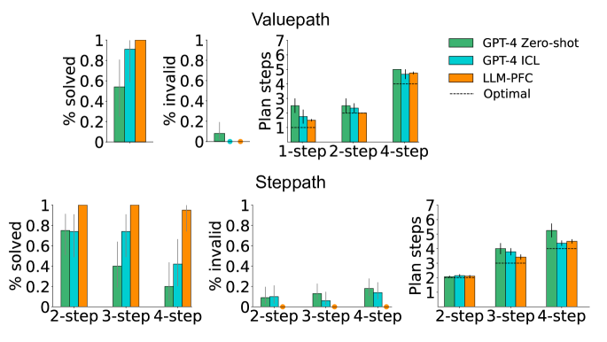
Figure 4: Graph traversal results. Top: Valuepath results. Bottom: Steppath results. Left: Fraction of solved problems (without proposing any invalid actions; $\uparrow$ better). Middle: fraction of invalid action proposals ($\downarrow$ better). Right: Plan length ($\downarrow$ better; note that these results only reflect problems that were successfully solved, and therefore exclude many problems for the baseline models). GPT-4 Zero-shot and ICL baselines are deterministic, and therefore a single run was performed on all problems. Note that LLM-PFC did not employ tree search on the Steppath task, and did not employ task decomposition on either task, as the performance of the model was already at ceiling without these components. Without tree search, LLM-PFC’s performance is deterministic, and therefore only a single run was performed on the Steppath task. Gray error bars reflect 95% binomial confidence intervals (for models evaluated on a single run). For Valuepath, we performed 5 runs with LLM-PFC, and present average performance $\pm$ the standard error of the mean (black error bars).

Figure 4 shows the results on the Valuepath and Steppath graph traversal tasks (see Section A.1 for all results in Table form). On the Valuepath task, LLM-PFC solved 100% of problems and proposed no invalid actions (e.g., it did not hallucinate the presence of non-existent edges), significantly outperforming both baselines. On the Steppath task, LLM-PFC displayed perfect performance for 2-step and 3-step paths, and near-perfect performance for 4-step paths, again significantly outperforming both baselines. The model also did not propose any invalid actions on this task. Notably, LLM-PFC’s proposed plans were close to the optimal number of steps for both tasks.

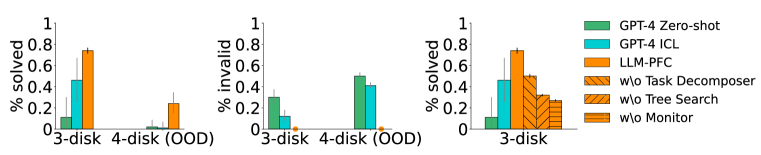
Figure 5: Tower of Hanoi (ToH) results. Left: Fraction of solved problems (without proposing any invalid actions; $\uparrow$ better). Middle: Fraction of invalid action proposals ($\downarrow$ better). Right: Ablation results for 3-disk problems ($\uparrow$ better). Note that 4-disk problems are out-of-distribution (OOD). GPT-4 Zero-shot and ICL baselines are deterministic and reflect a single run. Gray error bars reflect 95% binomial confidence intervals. Dots reflect values of 0%. LLM-PFC results for 3-disk problems reflect the average over 5 runs $\pm$ the standard error of the mean (black error bars). LLM-PFC results for 4-disk problems reflect a single run, due to the high computational cost of multiple runs.

Figure 5 shows the results on Tower of Hanoi (ToH). LLM-PFC demonstrated a significant improvement both in terms of the number of problems solved (left) and the number of invalid actions proposed (middle). On 3-disk problems, LLM-PFC yielded a nearly seven-fold improvement in the number of problems solved over zero-shot performance, and also significantly outperformed standard in-context learning (ICL). For the problems that LLM-PFC solved, the average plan length (5.4) was close to the optimal number of moves (4.4). The model also demonstrated some ability to generalize out-of-distribution (OOD) to more complex 4-disk problems (not observed in any in-context examples), whereas GPT-4 Zero-shot and GPT-4 ICL solved close to 0% of these problems. Notably, LLM-PFC did not propose any invalid actions, even on OOD 4-disk problems, whereas GPT-4 Zero-shot and ICL baselines both proposed a significant number of invalid actions.

4.1 Ablation Study

We also carried out an ablation study to determine the relative importance of each of LLM-PFC’s major components, focusing on the 3-disk ToH problems. Figure 5 (right) shows the results. We found that the $\operatorname{Monitor}$ was the most important component, as ablating this module resulted in significantly fewer solved problems, due primarily to an increased tendency to propose invalid moves (31% invalid moves vs. 0% for other ablation models). Ablating the tree search and $\operatorname{TaskDecomposer}$ module also resulted in significantly fewer solved problems. Overall, these results suggest that all major components played an important role in the model’s performance.

5 Related Work

Early work in AI formalized planning as a problem of search through a combinatorial state space, typically utilizing various heuristic methods to make this search tractable (Newell & Simon, 1956; Newell et al., 1959). Problems such as ToH figured prominently in this early research (Simon, 1975), as it affords the opportunity to explore ideas based on hierarchical or recursive planning (in which a larger problem is decomposed into a set of smaller problems). Our proposed architecture adopts some of the key ideas from this early work, including tree search and hierarchical planning.

A few recent studies have investigated planning in LLMs. These studies suggest that, although LLMs can perform relatively simple planning tasks (Huang et al., 2022), and can learn to make more complex plans given extensive domain-specific fine-tuning (Pallagani et al., 2022; Wu et al., 2023), they struggle on tasks that require zero-shot or few-shot generation of complex multi-step plans (Valmeekam et al., 2023; Momennejad et al., 2023). These results also align with studies that have found poor performance in tasks that involve other forms of extended multi-step reasoning, such as arithmetic (Dziri et al., 2023). Our approach is in large part motivated by the poor planning and reasoning performance exhibited by LLMs in these settings.

Some recent approaches have employed various forms of heuristic search to improve performance in LLMs (Lu et al., 2021; Zhang et al., 2023), but these approaches have generally involved search at the level of individual tokens. This is in contrast to our approach, in which search is performed at the more abstract level of task states (described in natural language). This is similar to other recently proposed black-box approaches in which ‘thoughts’ – meaningful chunks of natural language – are utilized as intermediate computations to solve more complex problems. These approaches include scratchpads (Nye et al., 2021), chain-of-thought (Wei et al., 2022b), tree-of-thoughts (Yao et al., 2023), reflexion (Shinn et al., 2023), Society of Mind (Du et al., 2023), and Describe-Explain-Plan-Select (Wang et al., 2023). All of these approaches can be viewed as implementing a form of controlled, or ‘system 2’, processing (as contrasted with automatic, or ‘system 1’, processing) (Schneider & Shiffrin, 1977; Sloman, 1996; Kahneman, 2011). In the brain, these controlled processes are strongly associated with the prefrontal cortex (Miller & Cohen, 2001). Therefore, in the present work, we leveraged knowledge from cognitive neuroscience about the modular properties of the PFC. The resulting architecture shares some components with other black box approaches (e.g., tree search (Yao et al., 2023)), but also introduces a number of new components (error monitoring, task decomposition, task coordination, state/action distinction), and combines these components in a novel manner inspired by the functional organization of the human brain.

There have also been a number of proposals for incorporating modularity into deep learning systems, including neural module networks (Andreas et al., 2016), and recurrent independent mechanisms (Goyal et al., 2019). Our approach is distinguished from these approaches by the proposal of modules that perform specific high-level component processes, based on knowledge of specific subregions within the PFC. Finally, our approach is closely related to a recent proposal to augment deep learning systems with PFC-inspired mechanisms (Russin et al., 2020). LLM-PFC can be viewed as a concrete framework for accomplishing this goal.

6 Conclusion and Future Directions

In this work, we have proposed the LLM-PFC architecture, an approach aimed at improving the planning ability of LLMs by taking inspiration from the modular architecture of the human PFC. In experiments on two challenging planning domains, graph traversal and Tower of Hanoi, we found that LLM-PFC significantly improved planning performance over standard LLM methods. While these results represent a significant step forward, there is still room for improvement: first, there are more challenging planning tasks (including shortcuts and detour) in Momennejad et al. (2023), which remain to be the topic of future applications of LLM-PFC; and second, the model has less than optimal performance on Tower of Hanoi. This may be due in part to the inherent limitations of prompting and in-context learning as methods for the specialization of LLM-PFC’s modules. A promising avenue for further improvement may be to jointly fine-tune the modules across a range of diverse tasks (which requires open-source models), rather than relying only on black box methods (our only option with GPT-4). A white-box approach would also eliminate the need for task-specific prompts, and potentially enable zero-shot planning on novel tasks. We look forward to investigating these possibilities in future work.

Appendix A Appendix

A.1 Results Tables

Table 1: Results on Valuepath task.

Model	Fraction solved problems	Fraction invalid actions	Avg plan steps
			1-step	2-step	4-step
GPT-4 Zero-shot	0.54	0.08	2.5	2.5	5
GPT-4 ICL	0.91	0.0	1.75	2.33	4.67
LLM-PFC	1.0	0.0	1.5	2	4.75

Table 2: Results on Steppath task.

Model	Fraction solved problems			Fraction invalid actions			Avg plan steps
	2-step	3 step	4-step	2-step	3-step	4-step	2-step	3-step	4-step
GPT-4 Zero-shot	0.75	0.4	0.2	0.09	0.13	0.18	2.07	4	5.25
GPT-4 ICL	0.74	0.74	0.42	0.10	0.06	0.14	2.14	3.78	4.38
LLM-PFC	1.0	1.0	0.95	0.0	0.0	0.0	2.1	3.42	4.5

Table 3: Results on ToH.

Model	Fraction solved problems		Fraction invalid actions
	3-disk	4-disk (OOD)	3-disk	4-disk (OOD)
GPT-4 Zero-shot	0.11	0.02	0.30	0.50
GPT-4 ICL	0.46	0.01	0.12	0.41
LLM-PFC	0.74	0.24	0.0	0.0

Table 4: Ablation study on ToH with 3 disks.

Model	Fraction solved problems	Fraction invalid actions
LLM-PFC	0.74	0.0
w/o Task Decomposer	0.50	0.0
w/o Tree Search	0.32	0.0
w/o Monitor	0.27	0.31

A.2 Prompts and in-context examples

A.2.1 Task Decomposer

For ToH, the $\operatorname{TaskDecomposer}$ generated a single subgoal per problem. The in-context examples included chain-of-thought reasoning (Wei et al., 2022b) based on the goal recursion strategy (Simon, 1975) (Section A.2.1), which is sometimes provided to human participants in psychological studies of problem solving (Carpenter et al., 1990). The specific prompt and in-context examples are shown below:

Consider the following puzzle problem:

Problem description:
- There are three lists labeled A, B, and C.
- There is a set of numbers distributed among those three lists.
- You can only move numbers from the rightmost end of one list to the rightmost end of another list.
Rule #1: You can only move a number if it is at the rightmost end of its current list.
Rule #2: You can only move a number to the rightmost end of a list if it is larger than the other numbers in that list.
A move is valid if it satisfies both Rule #1 and Rule #2.
A move is invalid if it violates either Rule #1 or Rule #2.

Goal: The goal is to generate a single subgoal from the current configuration, that helps in reaching the goal configuration using minimum number of moves.

To generate subgoal use the goal recursion strategy. First if the smallest number isn’t at the correct position in list C, then set the subgoal of moving the smallest number to its correct position in list C.But before that, the numbers larger than the smallest number and present in the same list as the smallest number must be moved to a list other than list C. This subgoal is recursive because in order to move the next smallest number to the list other than list C, the numbers larger than the next smallest number and present in the same list as the next smallest number must be moved to a list different from the previous other list and so on.

Note in the subgoal configuration all numbers should always be in ascending order in all the three lists.

Here are two examples:

Example 1:

This is the current configuration:
A = [0,1]
B = [2]
C = []

This is the goal configuration:
A = []
B = []
C = [0, 1, 2]

Answer:
I need to move 0 from list A to list C.
Step 1. Find the numbers to the right of 0 in list A. There is 1 to the right of 0.
Step 2. Find the numbers larger than 0 in list C. There are none.
I will move the numbers found in Step 1 and Step 2 to list B. Hence I will move 1 from list A to list B. Also numbers should be in ascending order in list B.
Subgoal:
A = [0]
B = [1, 2]
C = []

Example 2:

This is the current configuration:
A = [1]
B = [0]
C = [2]

This is the goal configuration:
A = []
B = []
C = [0, 1, 2]

Answer:
I need to move 0 from list B to list C.
Step 1. Find the numbers to the right of 0 in list B. There are none.
Step 2. Find the numbers larger than 0 in list C. There is 2 which is larger than 0.
I will move the numbers found in Step 1 and Step 2 to list A. Hence, I will move 2 from list C to list A. Also numbers should be in ascending order in list A.
Subgoal:
A = [1, 2]
B = [0]
C = []

Here is the task:

This is the current configuration:
A = [0, 1, 2]
B = []
C = []

This is the goal configuration:
A = []
B = []
C = [0, 1, 2]

Answer:

A.2.2 Actor

The $\operatorname{Actor}$ was prompted to propose $\displaystyle B=2$ distinct actions. In some instances, the $\operatorname{Actor}$ failed to propose two distinct actions. In those cases, we iteratively scaled the temperature by a factor of 0.1. This was done for a maximum of 10 attempts or until two distinct actions were produced. If the $\operatorname{Actor}$ was not able to propose two distinct actions even after 10 attempts, we then used only a single action. The specific prompt and in-context examples for the ToH task are shown below:

Consider the following puzzle problem:

Problem description:
- There are three lists labeled A, B, and C.
- There is a set of numbers distributed among those three lists.
- You can only move numbers from the rightmost end of one list to the rightmost end of another list.
Rule #1: You can only move a number if it is at the rightmost end of its current list.
Rule #2: You can only move a number to the rightmost end of a list if it is larger than the other numbers in that list.
A move is valid if it satisfies both Rule #1 and Rule #2.
A move is invalid if it violates either Rule #1 or Rule #2.

Goal: The goal is to end up in the goal configuration using minimum number of moves.

Here are two examples:

Example 1:

This is the starting configuration:
A = [0, 1]
B = [2]
C = []
This is the goal configuration:
A = []
B = []
C = [0, 1, 2]

Here is the sequence of minimum number of moves to reach the goal configuration from the starting configuration:

Move 2 from B to C.
A = [0, 1]
B = []
C = [2]

Move 1 from A to B.
A = [0]
B = [1]
C = [2]

Move 2 from C to B.
A = [0]
B = [1, 2]
C = []

Move 0 from A to C.
A = []
B = [1, 2]
C = [0]

Move 2 from B to A.
A = [2]
B = [1]
C = [0]

Move 1 from B to C.
A = [2]
B = []
C = [0, 1]

Move 2 from A to C.
A = []
B = []
C = [0, 1, 2]

Example 2:

This is the starting configuration:
A = [1]
B = [0]
C = [2]
This is the goal configuration:
A = []
B = []
C = [0, 1, 2]

Here is the sequence of minimum number of moves to reach the goal configuration from the starting configuration:

Move 2 from C to A.
A = [1, 2]
B = [0]
C = []

Move 0 from B to C.
A = [1, 2]
B = []
C = [0]

Move 2 from A to B.
A = [1]
B = [2]
C = [0]

Move 1 from A to C.
A = []
B = [2]
C = [0, 1]

Move 2 from B to C.
A = []
B = []
C = [0, 1, 2]

Here is the task:

This is the starting configuration:
A = [0, 1, 2]
B = []
C = []
This is the goal configuration:
A = [0]
B = [1, 2]
C = []

Give me only two different valid next moves possible from the starting configuration that would help in reaching the goal configuration using as few moves as possible.
Your answer should be in the format as below:
1. Move <N> from <src> to <trg>.

A.2.3 Monitor

The $\operatorname{Monitor}$ was prompted with chain-of-thought reasoning in which each of the rules of the task were checked before determining action validity. We stored the actions deemed valid by the $\operatorname{Monitor}$ in a separate buffer, and we terminated the action proposal loop (Algorithm  1) when there were two distinct actions in this buffer, or exceeded a maximum of 10 interactions with the $\operatorname{Monitor}$. After termination of the action proposal loop, if the buffer didn’t contain two distinct actions, we used the only action in the buffer. If the buffer was empty, we used the action(s) proposed by the $\operatorname{Actor}$ at the last attempt. The following text was used as a prompt and in-context examples in the ToH task:

Consider the following puzzle problem:

Problem description:
- There are three lists labeled A, B, and C.
- There is a set of numbers distributed among those three lists.
- You can only move numbers from the rightmost end of one list to the rightmost end of another list.
Rule #1: You can only move a number if it is at the rightmost end of its current list.
Rule #2: You can only move a number to the rightmost end of a list if it is larger than the other numbers in that list.
A move is valid if it satisfies both Rule #1 and Rule #2.
A move is invalid if it violates either Rule #1 or Rule #2.

Goal: The goal is to check if the proposed move satisfies or violates Rule #1 and Rule #2 and based on that if it is a valid or invalid move.

Here are two examples:

Example 1:

This is the initial configuration:
A = []
B = [1]
C = [0, 2]

Proposed move:
Move 0 from C to B.

Answer:
First check whether the move satisfies or violates Rule #1. Index of 0 in list C is 0. Length of list C is 2. The difference in length of list C and index of 0 in list C is 2, which is not equal to 1. Hence 0 is not at the rightmost end of list C, and the move violates Rule #1.
Next check whether the move satisfies or violates Rule #2. For that compute the maximum of list B, to which 0 is moved. Maximum of list B is 1. 0 is not larger than 1. Hence the move violates Rule #2.
Since the Move 0 from list C to list B violates both Rule #1 and Rule #2, it is invalid.

Example 2:

This is the initial configuration:
A = []
B = [1]
C = [0, 2]

Proposed move:
Move 2 from C to B.

Answer:
First check whether the move satisfies or violates Rule #1. Index of 2 in list C is 1. Length of list C is 2. The difference in length of list C and index of 2 in list C is 1. Hence 2 is at the rightmost end of list C, and the move satisfies Rule #1.
Next check whether the move satisfies or violates Rule #2. For that compute the maximum of list B, to which 2 is moved. Maximum of list B is 1. 2 is larger than 1. Hence the move satisfies Rule #2.
Since the Move 2 from list C to list B satisfies both Rule #1 and Rule #2, it is valid.

Here is the task:

This is the initial configuration:
A = []
B = [0, 1]
C = [2]

Proposed move:
Move 1 from B to A.

Answer:

A.2.4 Predictor

The $\operatorname{Predictor}$ was prompted to predict the next state, given the current state and the proposed action. The following text was used as a prompt and in-context examples in the ToH task:

Consider the following puzzle problem:

Problem description:
- There are three lists labeled A, B, and C.
- There is a set of numbers distributed among those three lists.
- You can only move numbers from the rightmost end of one list to the rightmost end of another list.
Rule #1: You can only move a number if it is at the rightmost end of its current list.
Rule #2: You can only move a number to the rightmost end of a list if it is larger than the other numbers in that list.

Goal: The goal is to predict the configuration of the three lists, if the proposed move is applied to the current configuration.

Here are two examples:

Example 1:

This is the current configuration:
A = []
B = [1]
C = [0, 2]

Proposed move:
Move 2 from list C to list B.

Answer:
A = []
B = [1, 2]
C = [0]

Example 2:

This is the current configuration:
A = []
B = [1]
C = [0, 2]

Proposed move:
Move 1 from list B to list A.

Answer:
A = [1]
B = []
C = [0, 2]

Here is the task:

This is the current configuration:
A = []
B = [0, 1]
C = [2]

Proposed move:
Move 1 from list B to list A.

Answer:

A.2.5 Evaluator

For the $\operatorname{Evaluator}$, in the ToH task, GPT-4 was prompted to generate a heuristic function that could be used to estimate the distance between the current state and the goal state. The description of this heuristic function was then included in the $\operatorname{Evaluator}$’s prompt. In the graph traversal tasks, we used only in-context examples, with no heuristic function prompt.

The following text shows prompt and in-context examples used in the ToH task. The first User message prompts GPT-4 to generate a heuristic function. After GPT-4’s response, another User message prompts the $\operatorname{Evaluator}$ to use this function:

USER: Consider the following puzzle problem:

Problem description:
- There are three lists labeled A, B, and C.
- There is a set of numbers distributed among those three lists.
- You can only move numbers from the rightmost end of one list to the rightmost end of another list.
Rule #1: You can only move a number if it is at the rightmost end of its current list.
Rule #2: You can only move a number to the rightmost end of a list if it is larger than the other numbers in that list.
A move is valid if it satisfies both Rule #1 and Rule #2.
A move is invalid if it violates either Rule #1 or Rule #2.

Goal: The goal is to predict the minimum number of valid moves required to reach the goal configuration from the current configuration.

Here are two examples:

Example 1:

This is the current configuration:
A = [0, 1, 2]
B = []
C = []

This is the goal configuration:
A = []
B = []
C = [0, 1, 2]

Answer:
The minimum number of valid moves required to reach the goal configuration from the current configuration is 7.

Example 2:

This is the current configuration:
A = [1, 2]
B = [0]
C = []

This is the goal configuration:
A = []
B = []
C = [0, 1, 2]

Answer:
The minimum number of valid moves required to reach the goal configuration from the current configuration is 4.

What heuristic function can be used to estimate the minimum number of valid moves required to reach the goal configuration from a given current configuration?

GPT-4: A suitable heuristic function for this problem is the "sum of the distances" heuristic. This heuristic estimates the minimum number of valid moves required to reach the goal configuration by calculating the sum of the distances each number needs to travel to reach its final position in the goal configuration.

Here’s how the heuristic function works:

1. For each number in the current configuration, determine its current position (list and index) and its goal position (list and index) in the goal configuration.
2. Calculate the distance between the current position and the goal position for each number. The distance can be calculated as the absolute difference between the indices of the current and goal positions, plus a penalty if the number needs to move to a different list.
3. Sum the distances calculated in step 2 for all numbers.

The heuristic function will return the sum of the distances, which is an estimate of the minimum number of valid moves required to reach the goal configuration from the current configuration.

This heuristic is admissible because it never overestimates the cost of reaching the goal configuration. It considers the minimum number of moves required for each number to reach its goal position, without taking into account the constraints imposed by the rules of the puzzle. Therefore, the actual number of moves required to reach the goal configuration will always be greater than or equal to the heuristic value.

USER: This is the current configuration:
A = [0]
B = []
C = [1, 2]
This is the goal configuration:
A = [0]
B = [1, 2]
C = []

Use the heuristic function to predict the minimum number of valid moves required to reach the goal configuration from the current configuration.

Please provide your answer according to the heuristic function in the format as below:
The minimum number of valid moves required to reach the goal configuration from the current configuration is <N>.

A.2.6 Task Coordinator

The $\operatorname{TaskCoordinator}$ was prompted to determine whether the current subgoal was achieved by the current state. The following text was used as a prompt and in-context examples in the ToH task:

Consider the following puzzle problem:

Problem description:
- There are three lists labeled A, B, and C.
- There is a set of numbers distributed among those three lists.
- You can only move numbers from the rightmost end of one list to the rightmost end of another list.
Rule #1: You can only move a number if it is at the rightmost end of its current list.
Rule #2: You can only move a number to the rightmost end of a list if it is larger than the other numbers in that list.

Goal: The goal is to predict whether the current configuraton matches the goal configuration or not.

Here are two examples:

Example 1:

This is the current configuration:
A = []
B = []
C = [0, 1, 2]

This is the goal configuration:
A = []
B = []
C = [0, 1, 2]

Answer: The current configuraton matches the goal configuration. Hence yes.

Example 2:

This is the current configuration:
A = [0, 1]
B = [2]
C = []

This is the goal configuration:
A = []
B = []
C = [0, 1, 2]

Answer: The current configuraton doesn’t match the goal configuration. Hence no.

Here is the task:

This is the current configuration:
A = []
B = [0, 1, 2]
C = []

This is the goal configuration:
A = []
B = []
C = [0, 1, 2]

Answer:

References

- Andreas et al. (2016) Jacob Andreas, Marcus Rohrbach, Trevor Darrell, and Dan Klein. Neural module networks. In Proceedings of the IEEE conference on computer vision and pattern recognition, pp. 39–48, 2016.
- Behrens et al. (2018) Timothy EJ Behrens, Timothy H Muller, James CR Whittington, Shirley Mark, Alon B Baram, Kimberly L Stachenfeld, and Zeb Kurth-Nelson. What is a cognitive map? organizing knowledge for flexible behavior. Neuron, 100(2):490–509, 2018.
- Botvinick et al. (1999) Matthew Botvinick, Leigh E Nystrom, Kate Fissell, Cameron S Carter, and Jonathan D Cohen. Conflict monitoring versus selection-for-action in anterior cingulate cortex. Nature, 402(6758):179–181, 1999.
- Brown et al. (2020) Tom Brown, Benjamin Mann, Nick Ryder, Melanie Subbiah, Jared D Kaplan, Prafulla Dhariwal, Arvind Neelakantan, Pranav Shyam, Girish Sastry, Amanda Askell, et al. Language models are few-shot learners. Advances in neural information processing systems, 33:1877–1901, 2020.
- Brunec & Momennejad (2022) Iva K Brunec and Ida Momennejad. Predictive representations in hippocampal and prefrontal hierarchies. Journal of Neuroscience, 42(2):299–312, 2022.
- Bubeck et al. (2023) Sébastien Bubeck, Varun Chandrasekaran, Ronen Eldan, Johannes Gehrke, Eric Horvitz, Ece Kamar, Peter Lee, Yin Tat Lee, Yuanzhi Li, Scott Lundberg, et al. Sparks of artificial general intelligence: Early experiments with gpt-4. arXiv preprint arXiv:2303.12712, 2023.
- Carpenter et al. (1990) Patricia A Carpenter, Marcel A Just, and Peter Shell. What one intelligence test measures: a theoretical account of the processing in the raven progressive matrices test. Psychological review, 97(3):404, 1990.
- Daw et al. (2005) Nathaniel D Daw, Yael Niv, and Peter Dayan. Uncertainty-based competition between prefrontal and dorsolateral striatal systems for behavioral control. Nature neuroscience, 8(12):1704–1711, 2005.
- Devlin et al. (2090) Jacob Devlin, Ming-Wei Chang, Kenton Lee, and Kristina Toutanova. Bert: Pre-training of deep bidirectional transformers for language understanding. Proceedings of NAACL-HLT, 17:4171–4186, 2090.
- Doll et al. (2015) Bradley B Doll, Katherine D Duncan, Dylan A Simon, Daphna Shohamy, and Nathaniel D Daw. Model-based choices involve prospective neural activity. Nature neuroscience, 18(5):767–772, 2015.
- Du et al. (2023) Yilun Du, Shuang Li, Antonio Torralba, Joshua B Tenenbaum, and Igor Mordatch. Improving factuality and reasoning in language models through multiagent debate. arXiv preprint arXiv:2305.14325, 2023.
- Dziri et al. (2023) Nouha Dziri, Ximing Lu, Melanie Sclar, Xiang Lorraine Li, Liwei Jian, Bill Yuchen Lin, Peter West, Chandra Bhagavatula, Ronan Le Bras, Jena D Hwang, et al. Faith and fate: Limits of transformers on compositionality. arXiv preprint arXiv:2305.18654, 2023.
- Fincham et al. (2002) Jon M Fincham, Cameron S Carter, Vincent van Veen, V Andrew Stenger, and John R Anderson. Neural mechanisms of planning: a computational analysis using event-related fmri. Proceedings of the National Academy of Sciences, 99(5):3346–3351, 2002.
- Goel & Grafman (1995) Vinod Goel and Jordan Grafman. Are the frontal lobes implicated in “planning” functions? interpreting data from the tower of hanoi. Neuropsychologia, 33(5):623–642, 1995.
- Goyal et al. (2019) Anirudh Goyal, Alex Lamb, Jordan Hoffmann, Shagun Sodhani, Sergey Levine, Yoshua Bengio, and Bernhard Schölkopf. Recurrent independent mechanisms. arXiv preprint arXiv:1909.10893, 2019.
- Huang et al. (2022) Wenlong Huang, Pieter Abbeel, Deepak Pathak, and Igor Mordatch. Language models as zero-shot planners: Extracting actionable knowledge for embodied agents. In International Conference on Machine Learning, pp. 9118–9147. PMLR, 2022.
- Kahneman (2011) Daniel Kahneman. Thinking, fast and slow. macmillan, 2011.
- Lu et al. (2021) Ximing Lu, Sean Welleck, Peter West, Liwei Jiang, Jungo Kasai, Daniel Khashabi, Ronan Le Bras, Lianhui Qin, Youngjae Yu, Rowan Zellers, et al. Neurologic a* esque decoding: Constrained text generation with lookahead heuristics. arXiv preprint arXiv:2112.08726, 2021.
- Mahowald et al. (2023) Kyle Mahowald, Anna A Ivanova, Idan A Blank, Nancy Kanwisher, Joshua B Tenenbaum, and Evelina Fedorenko. Dissociating language and thought in large language models: a cognitive perspective. arXiv preprint arXiv:2301.06627, 2023.
- Mattar & Lengyel (2022) Marcelo G Mattar and Máté Lengyel. Planning in the brain. Neuron, 110(6):914–934, 2022.
- Miller & Cohen (2001) Earl K Miller and Jonathan D Cohen. An integrative theory of prefrontal cortex function. Annual review of neuroscience, 24(1):167–202, 2001.
- Momennejad & Haynes (2012) I Momennejad and J D Haynes. Human anterior prefrontal cortex encodes the ‘what’and ‘when’of future intentions. Neuroimage, 2012.
- Momennejad et al. (2018) I Momennejad, A R Otto, N D Daw, and K A Norman. Offline replay supports planning in human reinforcement learning. Elife, 2018.
- Momennejad (2020) Ida Momennejad. Learning structures: Predictive representations, replay, and generalization. Current Opinion in Behavioral Sciences, 32:155–166, April 2020.
- Momennejad & Haynes (2013) Ida Momennejad and John-Dylan Haynes. Encoding of prospective tasks in the human prefrontal cortex under varying task loads. J. Neurosci., 33(44):17342–17349, October 2013.
- Momennejad et al. (2023) Ida Momennejad, Hosein Hasanbeig, Felipe Vieira Frujeri, Hiteshi Sharma, Robert Osazuwa Ness, Nebojsa Jojic, Hamid Palangi, and Jonathan Larson. Evaluating cognitive maps in large language models with cogeval: No emergent planning. In Advances in neural information processing systems, volume 37, 2023. URL https://arxiv.org/abs/2309.15129.
- Newell & Simon (1956) Allen Newell and Herbert Simon. The logic theory machine–a complex information processing system. IRE Transactions on information theory, 2(3):61–79, 1956.
- Newell et al. (1959) Allen Newell, John C Shaw, and Herbert A Simon. Report on a general problem solving program. In IFIP congress, volume 256, pp. 64. Pittsburgh, PA, 1959.
- Nye et al. (2021) Maxwell Nye, Anders Johan Andreassen, Guy Gur-Ari, Henryk Michalewski, Jacob Austin, David Bieber, David Dohan, Aitor Lewkowycz, Maarten Bosma, David Luan, et al. Show your work: Scratchpads for intermediate computation with language models. arXiv preprint arXiv:2112.00114, 2021.
- Owen (1997) Adrian M Owen. Cognitive planning in humans: neuropsychological, neuroanatomical and neuropharmacological perspectives. Progress in neurobiology, 53(4):431–450, 1997.
- Pallagani et al. (2022) Vishal Pallagani, Bharath Muppasani, Keerthiram Murugesan, Francesca Rossi, Lior Horesh, Biplav Srivastava, Francesco Fabiano, and Andrea Loreggia. Plansformer: Generating symbolic plans using transformers. arXiv preprint arXiv:2212.08681, 2022.
- Ramnani & Owen (2004) Narender Ramnani and Adrian M Owen. Anterior prefrontal cortex: insights into function from anatomy and neuroimaging. Nature reviews neuroscience, 5(3):184–194, 2004.
- Russin et al. (2020) Jacob Russin, Randall C O’Reilly, and Yoshua Bengio. Deep learning needs a prefrontal cortex. Work Bridging AI Cogn Sci, 107(603-616):1, 2020.
- Schapiro et al. (2013) Anna C Schapiro, Timothy T Rogers, Natalia I Cordova, Nicholas B Turk-Browne, and Matthew M Botvinick. Neural representations of events arise from temporal community structure. Nature neuroscience, 16(4):486–492, 2013.
- Schneider & Shiffrin (1977) Walter Schneider and Richard M Shiffrin. Controlled and automatic human information processing: I. detection, search, and attention. Psychological review, 84(1):1, 1977.
- Schuck et al. (2016) Nicolas W Schuck, Ming Bo Cai, Robert C Wilson, and Yael Niv. Human orbitofrontal cortex represents a cognitive map of state space. Neuron, 91(6):1402–1412, 2016.
- Shenhav et al. (2013) Amitai Shenhav, Matthew M Botvinick, and Jonathan D Cohen. The expected value of control: an integrative theory of anterior cingulate cortex function. Neuron, 79(2):217–240, 2013.
- Shinn et al. (2023) Noah Shinn, Beck Labash, and Ashwin Gopinath. Reflexion: an autonomous agent with dynamic memory and self-reflection. arXiv preprint arXiv:2303.11366, 2023.
- Simon (1975) Herbert A Simon. The functional equivalence of problem solving skills. Cognitive psychology, 7(2):268–288, 1975.
- Sloman (1996) Steven A Sloman. The empirical case for two systems of reasoning. Psychological bulletin, 119(1):3, 1996.
- Srivastava et al. (2022) Aarohi Srivastava, Abhinav Rastogi, Abhishek Rao, Abu Awal Md Shoeb, Abubakar Abid, Adam Fisch, Adam R Brown, Adam Santoro, Aditya Gupta, Adrià Garriga-Alonso, et al. Beyond the imitation game: Quantifying and extrapolating the capabilities of language models. arXiv preprint arXiv:2206.04615, 34:1877––1901, 2022.
- Tavares et al. (2015) Rita Morais Tavares, Avi Mendelsohn, Yael Grossman, Christian Hamilton Williams, Matthew Shapiro, Yaacov Trope, and Daniela Schiller. A map for social navigation in the human brain. Neuron, 87(1):231–243, 2015.
- Tolman (1948) Edward C Tolman. Cognitive maps in rats and men. Psychological review, 55(4):189, 1948.
- Valmeekam et al. (2023) Karthik Valmeekam, Matthew Marquez, Sarath Sreedharan, and Subbarao Kambhampati. On the planning abilities of large language models–a critical investigation. arXiv preprint arXiv:2305.15771, 2023.
- Wallis (2007) Jonathan D Wallis. Orbitofrontal cortex and its contribution to decision-making. Annu. Rev. Neurosci., 30:31–56, 2007.
- Wang et al. (2023) Zihao Wang, Shaofei Cai, Anji Liu, Xiaojian Ma, and Yitao Liang. Describe, explain, plan and select: Interactive planning with large language models enables open-world multi-task agents. arXiv preprint arXiv:2302.01560, 2023.
- Webb et al. (2023) Taylor Webb, Keith J Holyoak, and Hongjing Lu. Emergent analogical reasoning in large language models. Nature Human Behaviour, 7:1526––1541, 2023. URL https://doi.org/10.1038/s41562-023-01659-w.
- Wei et al. (2022a) Jason Wei, Yi Tay, Rishi Bommasani, Colin Raffel, Barret Zoph, Sebastian Borgeaud, Dani Yogatama, Maarten Bosma, Denny Zhou, Donald Metzler, Ed H. Chi, Tatsunori Hashimoto, Oriol Vinyals, Percy Liang, Jeff Dean, and William Fedus. Emergent abilities of large language models. Transactions on Machine Learning Research, 2022a. ISSN 2835-8856. URL https://openreview.net/forum?id=yzkSU5zdwD. Survey Certification.
- Wei et al. (2022b) Jason Wei, Xuezhi Wang, Dale Schuurmans, Maarten Bosma, Fei Xia, Ed Chi, Quoc V Le, Denny Zhou, et al. Chain-of-thought prompting elicits reasoning in large language models. Advances in Neural Information Processing Systems, 35:24824–24837, 2022b.
- Wu et al. (2023) Zhenyu Wu, Ziwei Wang, Xiuwei Xu, Jiwen Lu, and Haibin Yan. Embodied task planning with large language models. arXiv preprint arXiv:2307.01848, 2023.
- Wunderlich et al. (2012) Klaus Wunderlich, Peter Dayan, and Raymond J Dolan. Mapping value based planning and extensively trained choice in the human brain. Nature neuroscience, 15(5):786–791, 2012.
- Yao et al. (2023) Shunyu Yao, Dian Yu, Jeffrey Zhao, Izhak Shafran, Thomas L Griffiths, Yuan Cao, and Karthik Narasimhan. Tree of thoughts: Deliberate problem solving with large language models. arXiv preprint arXiv:2305.10601, 2023.
- Zhang et al. (2023) Shun Zhang, Zhenfang Chen, Yikang Shen, Mingyu Ding, Joshua B Tenenbaum, and Chuang Gan. Planning with large language models for code generation. arXiv preprint arXiv:2303.05510, 2023.