When is fast, implicit squaring of $A^{-1}B$ stable?

Abstract

We analyze Implicit Repeated Squaring (IRS) – an algorithm that implicitly computes $(A^{-1}B)^{2^{p}}$ for $A,B\in{\mathbb{C}}^{n\times n}$ and $p\in{\mathbb{N}}_{+}$. Originating with inverse-free divide-and-conquer eigensolvers, this routine uses only matrix multiplication and QR to produce $A_{p}$ and $B_{p}$ satisfying $A_{p}^{-1}B_{p}=(A^{-1}B)^{2^{p}}$. By offering the choice to work with $A_{p}$ and $B_{p}$ individually or form $A_{p}^{-1}B_{p}$, IRS is applicable to both implicit and explicit computations involving $(A^{-1}B)^{2^{p}}$. Moreover, it exhibits stability. In this paper, we present the first rigorous and general analysis of the algorithm, showing that a finite-arithmetic implementation of IRS – using any fast matrix multiplication routine – satisfies a mixed forward/backward stability bound provided $O(\log(1/\epsilon)+\log(\mu(n))+(p-1)\log(\kappa_{\text{IRS}}(A,B,p)))$ bits of precision are used, where $\epsilon$ is the desired (sufficiently small) forward error, $\mu(n)$ is a polynomial in $n$, and $\kappa_{\text{IRS}}$ is an appropriately chosen condition number. Hence, fast IRS is stable in relatively modest precision when $p$ is logarithmic in $n$ or smaller. We also demonstrate on a handful of examples that IRS offers improved accuracy over a naive algorithm that explicitly forms and squares $A^{-1}B$. Along the way, we develop a spectral norm perturbation bound for full QR that may be of independent interest.

Keywords: Repeated squaring, finite arithmetic, full QR, matrix exponential
  MSC Class: 65F60

1 Introduction

1.1 Motivation

We consider the task of computing $(A^{-1}B)^{2^{p}}$ for $A,B\in{\mathbb{C}}^{n\times n}$ and $p\in{\mathbb{N}}_{+}$, where $A$ is assumed to be invertible. This problem appears in a variety of computations in numerical linear algebra; we provide two examples as motivation.

1. Spectral Projectors. If $(A,B)$ is a regular matrix pencil, $(I+(A^{-1}B)^{2^{p}})^{-1}$ approaches a projector onto the eigenspace corresponding to eigenvalues that lie outside the unit disk. This can be seen by noting that $Av=\lambda Bv$ implies

   $$(I+(A^{-1}B)^{2^{p}})^{-1}v=\frac{\lambda^{2^{p}}}{\lambda^{2^{p}}+1}v.$$ (1.1.1)

   Provided $|\lambda|\neq 1$, squaring drives eigenvalues of $(I+(A^{-1}B)^{2^{p}})^{-1}$ to either zero or one, depending on their relation to the unit disk, without changing eigenvectors. This observation is the foundation of several divide-and-conquer solvers for the generalized eigenvalue problem [20, 3, 4, 13], each of which computes $(A^{-1}B)^{2^{p}}$ and subsequently a rank-revealing factorization of $(I+(A^{-1}B)^{2^{p}})^{-1}$.

2. Matrix Exponentials. The most commonly used algorithm for computing a matrix exponential is the scaling and squaring method [16]. This approach – implemented in Matlab as expm – is rooted in the observation

   $$e^{A}=(e^{(A/{2^{p}})})^{2^{p}}.$$ (1.1.2)

   By scaling $A$ so that $||A/2^{p}||_{2}$ is sufficiently small, a rational $[k/m]$ Padé approximation $e^{x}\approx\frac{p_{km}(x)}{q_{km}(x)}$ can be applied, where $p_{km}$ and $q_{km}$ are polynomials of degree $k$ and $m$ respectively. Using a diagonal approximation (meaning $k=m$), the exponential is then evaluated as

   $$e^{A}\approx\left[q_{mm}(A/2^{p})^{-1}p_{mm}(A/2^{p})\right]^{2^{p}}.$$ (1.1.3)

   While much effort has gone into evaluating the performance of scaling and squaring, and in particular devising best practices for choosing $p$ and the Padé approximation [2, 21, 1], the stability of the final squaring step of the algorithm has been largely overlooked.

The naive approach to computing $(A^{-1}B)^{2^{p}}$ involves explicitly forming $A^{-1}B$ and squaring it. Traditional numerical lore prompts some caution here; if $A$ is poorly conditioned, forming $A^{-1}B$ may introduce nontrivial error that will propagate as the resulting matrix is squared. With this in mind we ask: what other options for evaluating $(A^{-1}B)^{2^{p}}$ do we have and when are they stable?

1.2 Implicit Repeated Squaring (IRS)

In this paper, we focus on a QR-based alternative presented here as Algorithm 1 under the name Implicit Repeated Squaring (IRS). This routine originates with the spectral projector application discussed above, and in particular the divide-and-conquer algorithms of Bulgakov, Godunov, and Malyshev [9, 19, 20]. The name IRS is taken from Ballard, Demmel, and Dumitriu [4], who were the first to state it as a stand-alone subroutine as it appears here.

Algorithm 1 Implicit Repeated Squaring (IRS)
Input: $A,B\in{\mathbb{C}}^{n\times n}$ and $p$ a positive integer
Output: $A_{p},B_{p}\in{\mathbb{C}}^{n\times n}$ satisfying $A_{p}^{-1}B_{p}=(A^{-1}B)^{2^{p}}$

1:$A_{0}=A$

2:$B_{0}=B$

3:for $j=0:p-1$ do

4:     

$$\begin{pmatrix}B_{j}\\ -A_{j}\end{pmatrix} =\begin{pmatrix}Q_{11}&Q_{12}\\ Q_{21}&Q_{22}\end{pmatrix}\begin{pmatrix}R_{j}\\ 0\end{pmatrix}$$

$$A_{j+1} =Q_{12}^{H}A_{j}$$

$$B_{j+1} =Q_{22}^{H}B_{j}$$

5:end for

6:return $A_{p},B_{p}$

Each step of IRS is remarkably simple, consisting of one full QR factorization and two $n\times n$ matrix multiplications. Assuming invertibility where necessary, we can verify the squaring aspect of the algorithm by noting $Q_{12}^{H}B_{j}-Q_{22}^{H}A_{j}=0$, which implies $B_{j}A_{j}^{-1}=Q_{12}^{-H}Q_{22}^{H}$ and therefore

$$A_{j+1}^{-1}B_{j+1}=A_{j}^{-1}Q_{12}^{-H}Q_{22}^{H}B_{j}=A_{j}^{-1}(B_{j}A_{j}^{-1})B_{j}=(A_{j}^{-1}B_{j})^{2}.$$ (1.2.1)

Of course, IRS does not compute $(A^{-1}B)^{2^{p}}$ but rather two matrices $A_{p}$ and $B_{p}$ with $A_{p}^{-1}B_{p}=(A^{-1}B)^{2^{p}}$. For this reason, IRS is a particularly good candidate when the computation involving $(A^{-1}B)^{2^{p}}$ can be done without explicitly forming $A_{p}^{-1}B_{p}$. Such is the case in the spectral projector application, where $(A_{p}+B_{p})^{-1}A_{p}=(I+(A^{-1}B)^{2^{p}})^{-1}$ and an implicit rank-revealing factorization can be used (for example [5]). Even when this is not the case, IRS is still viable; while computing $A_{p}^{-1}B_{p}$ is subject to the same numerical stability concerns as computing $A^{-1}B$, the absence of further squaring means IRS may come out ahead in the long run. Framed another way, both IRS and the naive approach require one matrix inversion, though the placement of that inversion in the overall algorithm may improve/hinder performance.
Despite its broader applicability, IRS has to our knowledge exclusively been studied in terms of spectral projectors (most notably by Malyshev [20] and Bai, Demmel, and Gu [3]). We pursue a more rigorous and general error analysis in this paper in the hopes of filling this gap.

1.3 Model of Computation

To obtain a more comprehensive error bound, we work with IRS in finite arithmetic. Here, we review the basics of this model of computation as well as the notions of numerical stability that will be relevant.
Throughout, we assume a floating point (i.e., finite) arithmetic where

$$fl(x\circ y)=(x\circ y)(1+\Delta),\;\;|\Delta|\leq{\bf u}$$ (1.3.1)

for basic operations $\circ\in\left\{+,-,\times,\div\right\}$ and a machine precision ${\bf u}(\epsilon,n)$, which is a function of the desired accuracy $\epsilon$ and the size of the problem $n$. This is a standard formulation for finite-arithmetic computations (see for example [15]). Given ${\bf u}$, the number of bits of precision required to achieve (1.3.1) is $\log_{2}(1/{\bf u})$.
If $\text{alg}(x)$ is a finite-arithmetic implementation of an algorithm that computes $f(x)$, we distinguish between two measures of accuracy, which are also standard.

1. Forward Error: $||\text{alg}(x)-f(x)||$

2. Backward Error: $||x-\tilde{x}||$ for $\tilde{x}$ satisfying $\text{alg}(x)=f(\tilde{x})$.

Normwise stability for alg can defined by bounding these errors in terms of ${\bf u}$ for arbitrary $x$. Classical examples include forward stability (forward error bounded by $\mu(n){\bf u}||f(x)||$), backward stability (backward error bounded by $\mu(n){\bf u}||x||$), and logarithmic stability (backward error bounded by $\kappa_{f}(x)^{\chi(n)}\mu(n){\bf u}||x||$), where $\mu(n)$ and $\chi(n)$ are polynomials in $n$ and $\log(n)$, respectively, and $\kappa_{f}(x)$ is an appropriate condition number.
Logarithmic stability originates with Demmel, Dumitriu, and Holtz [11], who defined it in terms of the forward error bound

$$||\text{alg}(x)-f(x)||\leq\kappa_{f}(x)^{\chi(n)+1}\mu(n){\bf u}||f(x)||.$$ (1.3.2)

We justify borrowing terminology here by noting that any algorithm satisfying our logarithmic backward-error condition also satisfies (1.3.2). This is a consequence of standard perturbation theory, which similarly implies a forward-error bound of $\kappa_{f}(x)\mu(n){\bf u}||f(x)||$ for any backwards-stable algorithm. Comparing these forward-error bounds yields Table 1, which shows the correspondence between classical notions of stability and precision.

Type of stability	Required ${\bf u}$	Required bits of precision $\log_{2}(1/{\bf u})$
Forward	$\epsilon/\mu(n)$	$\log_{2}(1/\epsilon)+\log_{2}(\mu(n))$
Backward	$\epsilon/(\kappa_{f}(x)\mu(n))$	$\log_{2}(1/\epsilon)+\log_{2}(\mu(n))+\log_{2}(\kappa_{f}(x))$
Logarithmic [11]	$\epsilon/(\kappa_{f}(x)^{\chi(n)+1}\mu(n))$	$\log_{2}(1/\epsilon)+\log_{2}(\mu(n))+(\chi(n)+1)\log_{2}(\kappa_{f}(x))$

Table 1: Required precision for an algorithm of a given (normwise) stability to compute $f(x)$ with forward error $\epsilon||f(x)||$. As in (1.3.2), $\mu(n)$ and $\chi(n)$ are polynomials in $n$ and $\log(n)$ and $\kappa_{f}(x)$ is a condition number.

While backwards stability is typically considered the gold standard in numerical linear algebra, even its weaker, logarithmic counterpart is difficult to show for modestly complicated algorithms. This is the reality of working in finite arithmetic: forward stability is incredibly strict, implying that accuracy is independent of conditioning, while both backward and logarithmic stability require that $\text{alg}(x)=f(\tilde{x})$ for some $\tilde{x}$, which may not be possible depending on the context. For this reason, we set aside these definitions and pursue instead a bound on the precision ${\bf u}$ required for alg to satisfy the following mixed forward/backward stability bound:

$$||\text{alg}(x)-f(\tilde{x})||\leq\epsilon||x||\;\;\text{for some}\;\;||x-\tilde{x}||\leq\mu(n){\bf u}||x||.$$ (1.3.3)

Informally, our goal is to quantify the precision needed for alg to accurately compute $f$ on a nearby input $\tilde{x}$. We can draw a comparison between such a precision requirement and classical forward/backward/logarithmic stability via Table 1.

Remark 1.1.

The $||x||$ in the forward component of (1.3.3) is not a typo. While this is not a meaningful way to measure approximate forward error in general, as $||x||$ and $||f(x)||$ may differ significantly, it is usable here since the outputs of exact, implicit repeated squaring have norm at most that of the inputs. Said another way, $||f(x)||\leq||x||$ for repeated squaring, meaning the forward bound in (1.3.3) is simply a weaker version of $||\text{alg}(x)-f(\tilde{x})||\leq\epsilon||f(x)||$ for our purposes.

With this as a backdrop, we now state the finite-arithmetic black-box algorithms we assume access to in IRS alongside their error guarantees. Following the notation above, $\mu_{\text{MM}}(n)$ and $\mu_{\text{QR}}(n)$ are polynomials in $n$.

Assumption 1.2.

There exists a $n\times n$ matrix multiplication algorithm ${\bf MM}(\cdot,\cdot)$ satisfying

$$||{\bf MM}(A,B)-AB||_{2}\leq\mu_{\text{MM}}(n){\bf u}||A||_{2}||B||_{2}$$ (1.3.4)

in $T_{\text{MM}}(n)$ arithmetic operations.

Assumption 1.3.

There exists a full QR algorithm ${\bf QR}(\cdot)$ that satisfies the following in $T_{\text{QR}}(n)$ arithmetic operations.

1. $[Q,R]={\bf QR}(A)$ for $A,R\in{\mathbb{C}}^{2n\times n}$ and $Q\in{\mathbb{C}}^{2n\times 2n}$.

2. $R$ is exactly upper triangular with real diagonal entries.

3. There exist $A^{\prime}\in{\mathbb{C}}^{2n\times n}$ and unitary $Q^{\prime}\in{\mathbb{C}}^{2n\times 2n}$ such that $A^{\prime}=Q^{\prime}R$ with

   $$||Q-Q^{\prime}||_{2}\leq\mu_{\text{QR}}(n){\bf u}\;\;\text{and}\;\;||A-A^{\prime}||_{2}\leq\mu_{\text{QR}}(n){\bf u}||A||_{2}.$$ (1.3.5)

Once again, these black-box assumptions are somewhat standard [15, Section 3.5 and Chapter 19]. While we won’t be too particular about $\mu_{\text{MM}}(n)$ and $\mu_{\text{QR}}(n)$, we do note that they are compatible with fast matrix multiplication – i.e., QR can be implemented stably (in a mixed sense) using fast matrix multiplication [11], which itself can be formulated to satisfy the forward error bound given by 1.2 [12]. Consequently our analysis applies to IRS implemented with a variety of fast matrix multiplication routines [25, 10, 28], including the current fastest known algorithm of Williams et al. [29], and we may additionally assume $T_{\text{QR}}(n)=O(T_{\text{MM}}(n))$.

1.4 Results

Our main contribution – presented in full detail as 3.6 – can be summarized informally as follows.

Main Result.

Let $\mu(n)=\max\left\{\mu_{\text{MM}}(n),\mu_{\text{QR}}(n)\right\}$, $A,B\in{\mathbb{C}}^{n\times n}$, and $p\in{\mathbb{N}}_{+}$. The finite-arithmetic outputs $[A_{p},B_{p}]={\textbf{IRS}}(A,B,p)$ satisfy a mixed stability bound, as defined in (1.3.3), for $\epsilon>0$ sufficiently small (depending on $A$, $B$, and $p$) provided

$${\bf u}=O\left(\frac{\epsilon}{\mu(n)(\log(n)\kappa_{\text{IRS}}(A,B,p))^{p-1}}\right),$$

where $\kappa_{\text{IRS}}$ is the condition number defined in Section 2.2. Hence, finite-arithmetic IRS requires

$$\log\left(\frac{1}{\epsilon}\right)+\log(\mu(n))+(p-1)(\log(\kappa_{\text{IRS}}(A,B,p))+\log(\log(n)))$$

bits of precision to compute $A_{p}$ and $B_{p}$ stably.

This result allows us to distinguish regions of stability for IRS based on the number of steps taken: when $p$ is a small constant IRS exhibits an analog of backwards stability (up to $\log(\log(n))$ factors), while a logarithmic number of steps requires a corresponding logarithmic increase in the number of bits. In Section 4, we demonstrate on a handful of examples that this stability is inherited by $A_{p}^{-1}B_{p}$ in many cases.
The remainder of the paper is organized as follows. In Section 2 we lay the groundwork for our analysis by developing some intermediate results, most notably a QR perturbation bound (2.13). We follow that by proving our main result in Section 3 and exploring the aforementioned numerical examples in Section 4. In Appendix A, we consider how the mixed stability bound available to IRS can be extended to a theoretical forward error bound for computing $(A^{-1}B)^{2^{p}}$ explicitly.

2 Tools from Linear Algebra

In this section, we discuss a handful of intermediate results that will be useful in the subsequent analysis. Here and in the remainder of the paper, $||\cdot||_{2}$ and $||\cdot||_{F}$ denote the spectral and Frobenius norms, $\kappa_{2}(A)$ is the spectral norm condition number of $A$, and $\sigma_{i}(A)$ is the $i^{\text{th}}$ singular value of $A$. Additionally, $A^{H}$, $A^{-H}$, and $A^{\dagger}$ denote the Hermitian transpose, inverse Hermitian transpose, and pseudoinverse respectively.
Throughout, it will be convenient to make connections between the inputs of IRS and the eigenvalues of the corresponding pencil $(A,B)$. With this in mind, we note that $(A,B)$ is regular if $\det(A-\lambda B)$ is not identically zero and is singular otherwise. Standard background references for matrix pencils and the generalized eigenvalue problem include [24, 17].

2.1 Singular Value Inequalities

We begin with a few singular value inequalities. For completeness, we sketch the proofs.

Lemma 2.1.

Suppose $M=\binom{A\;\;B}{0\;\;C}\in{\mathbb{C}}^{m\times m}$ for $A\in{\mathbb{C}}^{n\times l}$ with $l\leq n$. Then $\sigma_{m}(M)\leq\sigma_{l}(A).$

Proof.

By the min-max theorem for singular values, we have

$$\sigma_{m}(M)=\min_{\begin{subarray}{c}x\in{\mathbb{C}}^{m}\\ ||x||_{2}=1\end{subarray}}||Mx||_{2}.$$ (2.1.1)

We obtain the desired inequality by restricting to the case where $x=(y^{T}\;\;0)^{T}$ for $y\in{\mathbb{C}}^{l}$ with $||y||_{2}=1$. ∎

Lemma 2.2.

Suppose $M=\binom{A\;\;B}{0\;\;C}\in{\mathbb{C}}^{m\times m}$ for $C\in{\mathbb{C}}^{k\times k}$. Then $\sigma_{m}(M)\leq\sigma_{k}(C).$

Proof.

This inequality can be obtained by showing $\sigma_{k}(C^{H})\leq\sigma_{k}(M^{H})$ via essentially the same argument used to prove 2.1. ∎

Note that these lemmas cannot apply simultaneously to the same $M$ unless $A$ is square. To wrap up, we state a perturbation result for singular values, which is consequence of Weyl’s inequality [24, §IV Corollary 4.9].

Lemma 2.3 (Stability of Singular Values).

For $M_{1},M_{2}\in{\mathbb{C}}^{n\times n}$,

$$|\sigma_{i}(M_{1})-\sigma_{i}(M_{2})|\leq||M_{1}-M_{2}||_{2}$$

for all $1\leq i\leq n$.

2.2 Condition Number

We next explore possible condition numbers for repeated squaring. Historically, IRS has been analyzed in terms of one of the following two quantities. First is $\omega_{(A,B)}$ – the “criterion of absence of eigenvalues of the pencil $\lambda B-A$ on the unit circle and within a small neighborhood of it” introduced by Malyshev [20]. While the formal definition of $\omega_{(A,B)}$ covers only regular pencils, it can be easily extended by setting $\omega_{(A,B)}=\infty$ when $(A,B)$ is singular.

Definition 2.4.

For a regular pencil $(A,B)$

$$\omega_{(A,B)}=\left|\left|\frac{1}{2}\int_{0}^{2\pi}(B-e^{i\phi}A)^{-1}(AA^{H}+BB^{H})(B-e^{i\phi}A)^{-H}d\phi\right|\right|_{2}.$$

Aiming to replace $\omega_{(A,B)}$ with something more straightforward (both computationally and conceptually) Bai, Demmel, and Gu [3] subsequently analyzed IRS in terms of distance to the nearest ill-posed problem $d_{(A,B)}$.

Definition 2.5.

The distance from $(A,B)$ to the nearest ill-posed problem is

$$d_{(A,B)}=\inf\left\{||E||_{2}+||F||_{2}:(A+E)-z(B+F)\;\;\text{is singular for some}\;\;|z|=1\right\}.$$

Both $\omega_{(A,B)}$ and $d_{(A,B)}$ are specialized to the setting where IRS is employed to compute spectral projectors. Indeed, Malyshev [20, Equation 23] and Bai, Demmel, and Gu [3, Theorem 1] bound the error in computing spectral projectors of $(A,B)$ via IRS in terms of $\omega_{(A,B)}$ and $\frac{1}{d_{(A,B)}}$ respectively. Moreover, $\omega_{(A,B)}$ and $\frac{1}{d_{(A,B)}}$ are infinite if $(A,B)$ is singular or has an eigenvalue on the unit circle, in which case squaring cannot successfully produce a projector by driving eigenvalues to zero and infinity. As a result, both have been cast as condition numbers for the procedure.
In general, $(A,B)$ having an eigenvalue on the unit circle is not necessarily a problem for IRS, where we are only interested in obtaining an approximation of $(A^{-1}B)^{2^{p}}$. With this in mind, letting $m=2^{p}$, we work instead with $\sigma_{\min}(M_{p}(A,B))$ for $M_{p}(A,B)$ the $mn\times mn$ block matrix

$$M_{p}(A,B)=\begin{pmatrix}-A&&&-B\\ B&-A&&\\ &\ddots&\ddots&\\ &&B&-A\end{pmatrix}.$$ (2.2.1)

Notably, it can be shown that $p$ steps of IRS is essentially equivalent to computing a block QR factorization of $M_{p}(A,B)$ [3, Section 7]. Moreover, $\sigma_{\min}(M_{p}(A,B))$ has a nice correspondence with both $d_{(A,B)}$ and $\omega_{(A,B)}$.

Lemma 2.6.

If $(A,B)$ is regular then

$$\sigma_{n}\binom{B}{-A}\geq\sigma_{\min}(M_{p}(A,B))\geq d_{(A,B)}>\frac{\sqrt{\sigma_{n}(AA^{H}+BB^{H})}}{14\omega_{(A,B)}}.$$

Proof.

The first inequality follows from 2.1 since $\sigma_{n}\binom{B}{-A}=\sigma_{n}\binom{-A}{B}$. The second is an observation of Bai, Demmel, and Gu. They show that $M_{p}(A,B)$ is unitarily equivalent to the $mn\times mn$ block diagonal matrix $\text{diag}(-A+e^{i\theta_{1}}B,\ldots,-A+e^{i\theta_{m}}B)$ for $e^{i\theta_{1}},\ldots e^{i\theta_{m}}$ the $m^{\text{th}}$ roots of $-1$. Consequently, since we also have $d_{(A,B)}=\min_{\theta}\sigma_{n}(-A+e^{i\theta}B)$,

$$\sigma_{\min}(M_{p}(A,B))=\min_{1\leq j\leq m}\sigma_{n}(-A+e^{i\theta_{j}}B)\geq\min_{\theta}\sigma_{n}(-A+e^{i\theta}B)=d_{(A,B)}.$$ (2.2.2)

The final inequality follows from [20, Theorem 3]. Letting $LL^{H}=AA^{H}+BB^{H}$ be a Cholesky factorization (which exists since $(A,B)$ is regular) and setting $A_{0}=L^{-1}A$ and $B_{0}=L^{-1}B$, we have

$$\frac{1}{14\omega_{(A,B)}}<\frac{1}{\max_{\phi}||(B_{0}-e^{i\phi}A_{0})^{-1}||_{2}}=\min_{\phi}\sigma_{n}(B_{0}-e^{i\phi}A_{0})\leq||L^{-1}||_{2}\min_{\phi}(B-e^{i\phi}A)=\frac{d_{(A,B)}}{\sigma_{n}(L)}.$$ (2.2.3)

We complete the proof by rearranging and recalling that $\sigma_{i}(L)^{2}=\sigma_{i}(AA^{H}+BB^{H})$ for all $i$. ∎

Importantly, 2.6 allows us to link our analysis to the previous work with only minor modifications. On top of this, $\sigma_{\min}(M_{p}(A,B))$ bounds the smallest singular value of the block matrix used at any step of exact-arithmetic IRS, meaning it can be used to control the condition number for each QR factorization.

Lemma 2.7.

Suppose $A_{j},B_{j}\in{\mathbb{C}}^{n\times n}$ is any pair of matrices obtained while applying $p$ steps of exact-arithmetic repeated squaring to $A$ and $B$. Then

$$\sigma_{n}\binom{B_{j}}{-A_{j}}\geq\sigma_{\min}(M_{p}(A,B)).$$

Proof.

In their analysis, Bai, Demmel, and Gu show that the block matrix

$$M_{p}^{(j)}(A,B)=\begin{pmatrix}\;\;\;\text{*}\;&\text{*}\\ \;\;\;0\;&\begin{pmatrix}-A_{j}&&&-B_{j}\\ B_{j}&-A_{j}&&\\ &\ddots&\ddots&\\ &&B_{j}&-A_{j}\end{pmatrix}\\ \end{pmatrix}$$ (2.2.4)

can be obtained from $M_{p}(A,B)$ by left multiplying by unitary matrices. Here, the lower right block is $nk\times nk$ for $k=2^{p-j}$ and the asterisk blocks are arbitrary (not necessarily zero). Since multiplying by unitary matrices does not change singular values, the result follows from applying, in order, 2.2 and 2.1. ∎

Like $d_{(A,B)}$, $\sigma_{\min}(M_{p}(A,B))$ is not invariant to scaling and is therefore not suitable to measure conditioning for repeated squaring on its own. Instead, we state our results in terms of

$$\kappa_{\text{IRS}}(A,B,p)\coloneqq\sigma_{\min}(M_{p}(A,B))^{-1}\left|\left|\binom{A}{B}\right|\right|_{2},$$ (2.2.5)

which is both invariant to scaling and satisfies $\kappa_{\text{IRS}}(A,B,p)=\kappa_{\text{IRS}}(B,A,p)$. It is also not difficult to show $\kappa_{\text{IRS}}(A,B,p)\geq 1$.
Recalling our motivation for defining a new condition number, we observe from the proof of 2.6 that $\kappa_{\text{IRS}}(A,B,p)$ is infinite if $(A,B)$ has an eigenvalue on the unit circle, though only if this eigenvalue is an $m^{\text{th}}$ root of $-1$. Unlike $\omega_{(A,B)}$ or $\frac{||(A\;B)||_{2}}{d_{(A,B)}}$, we can make sense of this without considering spectral projectors, as it indicates that the QR factorization of $M_{p}(A,B)$ computed by IRS is no longer uniquely determined.
We also note that, of the condition numbers considered here, $\kappa_{\text{IRS}}(A,B,p)$ is the only one to include an explicit dependence on $p$, the number of steps of squaring. While $\kappa_{\text{IRS}}(A,B,p)$ increases with $p$, 2.6 implies the $p$-independent upper bound

$$\kappa_{\text{IRS}}(A,B,p)\leq d_{(A,B)}^{-1}\left|\left|\binom{A}{B}\right|\right|_{2}.$$ (2.2.6)

Thinking of $p$ as an input to the procedure not only provides a sharper condition number – as shown here – but also allows us to quantify the stability of IRS in terms of the number of steps taken (and in particular its dependence on $n$).
To conclude this section, we verify a perturbation bound for $\sigma_{\min}(M_{p}(A,B))$ that will be useful later on.

Lemma 2.8.

Let $A,B$ and $\tilde{A},\tilde{B}$ be pairs of matrices with $||A-\tilde{A}||_{2},||B-\tilde{B}||_{2}\leq\delta$. Then for any $p\in{\mathbb{N}}_{+}$

$$\sigma_{\min}(M_{p}(\tilde{A},\tilde{B}))\geq\sigma_{\min}(M_{p}(A,B))-2\delta.$$

Proof.

Let $\tilde{A}=A+E$ and $\tilde{B}=B+F$ for $||E||_{2},||F||_{2}\leq\delta$. By 2.3 we have

$$\sigma_{\min}(M_{p}(\tilde{A},\tilde{B}))=\sigma_{\min}(M_{p}(A,B)+M_{p}(E,F))\geq\sigma_{\min}(M_{p}(A,B))-||M_{p}(E,F)||_{2}.$$ (2.2.7)

Recalling from the proof of 2.6 that $M_{p}(E,F)$ is unitarily equivalent to a block diagonal matrix of the form $\text{diag}(-E+e^{i\theta_{1}}F,\ldots,-E+e^{i\theta_{m}}F)$, we have

$$||M_{p}(E,F)||_{2}=\max_{1\leq j\leq m}||-E+e^{i\theta_{m}}F||_{2}\leq||E||_{2}+||F||_{2}=2\delta$$ (2.2.8)

and therefore $\sigma_{\min}(M_{p}(\tilde{A},\tilde{B}))\geq\sigma_{\min}(M_{p}(A,B))-2\delta$. ∎

2.3 Perturbation Theory for Full QR

With 2.7 in mind, we’ll next need some perturbation bounds for the $2n\times n$ QR factorizations computed by IRS. While perturbation theory for QR originates with Stewart [23], a standard result of Sun [26, Theorem 1.6] is our starting point.

Theorem 2.9 (Sun 1991).

Let $A\in{\mathbb{C}}^{m\times n}$ have rank $n$ and let $A=QR$ be a reduced QR factorization, where $Q\in{\mathbb{C}}^{m\times n}$ satisfies $Q^{H}Q=I_{n}$ and $R\in{\mathbb{C}}^{n\times n}$ has real, positive diagonal entries. If $E\in{\mathbb{C}}^{m\times n}$ satisfies $||A^{\dagger}||_{2}||E||_{2}<1$ then there exists a unique (reduced) QR factorization

$$(A+E)=(Q+W)(R+F)$$

such that

$$||W||_{F}\leq(1+\sqrt{2})\;\alpha(||A^{\dagger}||_{2}||E||_{2})\;\kappa_{2}(A)\;\frac{||E||_{F}}{||A||_{2}},$$

where $\alpha(\epsilon)=\frac{1}{\epsilon}\ln\left(\frac{1}{1-\epsilon}\right)$ for $0<\epsilon<1$.

There are two issues with using this result as is. First, it’s stated in terms of the Frobenius norm and is therefore less convenient than a spectral norm bound. We could convert between the two, but doing so naively will incur a factor of $\sqrt{n}$, which – as we will see – is more pessimistic than necessary. On top of this, 2.9 covers only reduced QR factorizations and therefore does not apply explicitly to those computed by IRS. Luckily, this can be addressed with the following lemma.

Lemma 2.10.

Let $Q=[Q_{1}\;Q_{2}]$ and $U=[U_{1},U_{2}]$ be two $2n\times 2n$ unitary matrices with $Q_{1},U_{1}\in{\mathbb{C}}^{2n\times n}$. If $||Q_{1}-U_{1}||_{2}\leq\delta$ then there exists a unitary $W\in{\mathbb{C}}^{n\times n}$ such that

$$||Q_{2}-U_{2}W||_{2}\leq 4\delta.$$

Proof.

Without loss of generality assume $\delta<\frac{1}{2}$ (the bound is trivial otherwise). We first note that we can use $||Q_{1}-U_{1}||_{2}$ to control the distance between the orthogonal projectors $Q_{1}Q_{1}^{H}$ and $U_{1}U_{1}^{H}$:

$$||Q_{1}Q_{1}^{H}-U_{1}U_{1}^{H}||_{2} =||Q_{1}Q_{1}^{H}-Q_{1}U_{1}^{H}+Q_{1}U_{1}^{H}-U_{1}U_{1}^{H}||_{2}$$ (2.3.1)

$$\leq||Q_{1}(Q_{1}-U_{1})^{H}||_{2}+||(Q_{1}-U_{1})U_{1}^{H}||_{2}$$

$$\leq 2||Q_{1}-U_{1}||_{2}$$

$$\leq 2\delta.$$

Since $Q_{2}Q_{2}^{H}=I-Q_{1}Q_{1}^{H}$ and $U_{2}U_{2}^{H}=I-U_{1}U_{1}^{H}$ this similarly implies $||Q_{2}Q_{2}^{H}-U_{2}U_{2}^{H}||_{2}\leq 2\delta$. With this in mind, let $Q_{1}Q_{1}^{H}=U_{1}U_{1}^{H}+E$ for some $E\in{\mathbb{C}}^{2n\times 2n}$ with $||E||_{2}\leq 2\delta$. Noting $Q_{2}Q_{2}^{H}=U_{2}U_{2}^{H}-E$ we observe

$$Q_{2}-U_{2}(U_{2}^{H}Q_{2})=-EQ_{2}.$$ (2.3.2)

Consider now $U_{2}^{H}Q_{2}$:

$$(U_{2}^{H}Q_{2})^{H}U_{2}^{H}Q_{2}=Q_{2}^{H}U_{2}U_{2}^{H}Q_{2}=Q_{2}^{H}(I-U_{1}U_{1}^{H})Q_{2}=I-Q_{2}^{H}(Q_{1}Q_{1}^{H}-E)Q_{2}=I+Q_{2}^{H}EQ_{2}.$$ (2.3.3)

(2.3.3) implies that each singular value of $U_{2}^{H}Q_{2}$ takes the form $\sqrt{1+\lambda}$ for $\lambda$ an eigenvalue of $Q_{2}^{H}EQ_{2}$ satisfying $|\lambda|\leq||Q_{2}^{H}EQ_{2}||_{2}\leq 2\delta$. Consequently, the SVD of $U_{2}^{H}Q_{2}$ can be written as

$$U_{2}^{H}Q_{2}=V_{1}(I+\Sigma)V_{2}^{H}$$ (2.3.4)

for $V_{1},V_{2}\in{\mathbb{C}}^{n\times n}$ unitary and $\Sigma$ diagonal with nonzero entries bounded in magnitude by $2\delta$. Letting $W=V_{1}V_{2}^{H}$ we have

$$Q_{2}-U_{2}W=-EQ_{2}+U_{2}V_{1}\Sigma V_{2}^{H}$$ (2.3.5)

where, by construction, $||-EQ_{2}+U_{2}V_{1}\Sigma V_{2}^{H}||_{2}\leq||E||_{2}+||\Sigma||_{2}\leq 4\delta.$ ∎

Informally, 2.10 says that the trailing columns of two full QR factorizations corresponding to nearby reduced ones are close to rotations/reflections of one another. Put another way, two nearby reduced factorizations can be built into similarly close full factorizations, which allows us to extend any reduced bound to full QR as it is used in IRS.
With this in mind, we now pursue a (sharper) spectral norm version of 2.9. Ostensibly, Sun’s result is written in terms of the Frobenius norm because it makes use of the following inequality: given $L\in{\mathbb{C}}^{n\times n}$ lower triangular with real diagonal entries,

$$||L||_{F}\leq\frac{1}{\sqrt{2}}||L+L^{H}||_{F}.$$ (2.3.6)

While no inequality of the form $||L||_{2}\leq C||L+L^{H}||_{2}$ for $C$ a positive constant can exist (multiply the matrix in [6, Example 3.3] by $i$ for a counterexample, as was pointed out to us by Anne Greenbaum [14]), we can prove the following alternative.

Lemma 2.11.

Let $L\in{\mathbb{C}}^{n\times n}$ be lower triangular with real diagonal entries. Then,

$$||L||_{2}\leq\left(\frac{1}{2}+L_{n+1}\right)||L+L^{H}||_{2}$$

for $L_{k}=\frac{1}{2\pi}\int_{-\pi}^{\pi}|D_{k}(\theta)|d\theta$ the $k^{\text{th}}$ Lebesgue constant and $D_{k}(\theta)$ the Dirichlet kernel.

Proof.

This follows from Bhatia [6]. Writing

$$L^{H}=\Delta_{U}(L+L^{H})-\frac{1}{2}{\mathcal{D}}_{0}(L+L^{H})$$ (2.3.7)

where $\Delta_{U}(A)$ and ${\mathcal{D}}_{0}(A)$ are obtained from $A$ be zeroing out the sub-diagonal and off-diagonal entries respectively, we have

$$||L||_{2}=||L^{H}||_{2}\leq||\Delta_{U}(L+L^{H})||_{2}+\frac{1}{2}||{\mathcal{D}}_{0}(L+L^{H})||_{2}\leq\left(\frac{1}{2}+L_{n+1}\right)||L+L^{H}||_{2}$$ (2.3.8)

after applying [6, Equations 3 and 15]. ∎

Remark 2.12.

It can be shown [7, Section 2.2] that

$$L_{k}\leq\ln(k)+\ln(\pi)+\frac{2}{\pi}\left(1+\frac{2}{k}\right).$$ (2.3.9)

In other words, $L_{k}$ grows (at most) like $\log(k)$ for large $k$ and 2.11 could be written generally as $||L||_{2}\leq O(\log(n))||L+L^{H}||_{2}$. In an effort to keep track of constants, we will use the explicit, though slightly looser,

$$||L||_{2}\leq(\ln(n+1)+3)||L+L^{H}||_{2}$$ (2.3.10)

going forward. Note that the counterexample mentioned above implies that the dependence on $\log(n)$ is tight.

Repeating the proof of [26, Theorem 1.6] with (2.3.10) in place of (2.3.6) yields the main perturbation bound we will use in the next section.

Theorem 2.13.

Let $A\in{\mathbb{C}}^{m\times n}$ have rank $n$ and let $A=QR$ be an reduced QR factorization, where $Q\in{\mathbb{C}}^{m\times n}$ satisfies $Q^{H}Q=I_{n}$ and $R\in{\mathbb{C}}^{n\times n}$ has real, positive diagonal entries. If $E\in{\mathbb{C}}^{m\times n}$ satisfies $||A^{\dagger}||_{2}||E||_{2}<1$ then there exists a unique (reduced) QR factorization

$$(A+E)=(Q+W)(R+F)$$

such that

$$||W||_{2}\leq(2\ln(n+1)+7)\ln\left(\frac{1}{1-||A^{\dagger}||_{2}||E||_{2}}\right)=(2\ln(n+1)+7)\;\alpha(||A^{\dagger}||_{2}||E||_{2})\;\kappa_{2}(A)\;\frac{||E||_{2}}{||A||_{2}},$$

for $\alpha(\epsilon)$ as in 2.9.

While to our knowledge this result is new, it not the only QR perturbation bound developed since 2.9. Sun himself provided improvements for real matrices only a few years later [27]. More general bounds were subsequently found by Bhatia and Mukherjea [8] and Li and Wei[18]. We also note a recent componentwise analysis done by Petkov [22], again for real matrices. Despite their improvements over 2.9, these results are not easily adaptable into a general, spectral norm bound – hence our choice to use 2.13 in the analysis to come.

3 Finite-Arithmetic Analysis

We now prove our main error bound for a finite-arithmetic implementation of IRS. To avoid any confusion, bold and capital letters always refer to finite-arithmetic computations in this section. In particular, we differentiate $AB$ – the exact-arithmetic product of $A$ and $B$ – from its finite-arithmetic counterpart $\textbf{MM}(A,B)$. Throughout, we also use the block notation $A=\binom{A_{11}\;A_{12}}{A_{21}\;A_{22}}$ to reference the main $n\times n$ blocks of any $2n\times 2n$ matrix $A$.
In terms of the black-box algorithms defined in Section 1.3, one iteration of IRS consists of the following three steps: 1. $[Q,R]=\textbf{QR}\binom{B_{j}}{-A_{j}}$; 2. $A_{j+1}=\textbf{MM}(Q_{12}^{H},A_{j})$; 3. $B_{j+1}=\textbf{MM}(Q_{22}^{H},B_{j})$. Note that we recycle the notation of $Q$ and $R$ here for simplicity; in practice these are different for each value of $j$. Throughout our analysis, we use the following pairs of matrices:

1. The inputs to IRS: $A_{0}=A$ and $B_{0}=B$.

2. The nearby inputs: $\tilde{A}_{0}$ and $\tilde{B}_{0}$. If $[Q,R]=\textbf{QR}\binom{B_{0}}{-A_{0}}$ is the first QR factorization computed by IRS, $\tilde{A}_{0}$ and $\tilde{B}_{0}$ are the pair satisfying

   $$\binom{\tilde{B}_{0}}{-\tilde{A}_{0}}=\tilde{Q}R$$ (3.0.1)

   for $||Q-\tilde{Q}||_{2}\leq\mu_{\text{QR}}(n){\bf u}$, which are guaranteed to exist by 1.3. Moreover,

   $$||A_{0}-\tilde{A}_{0}||_{2},||B_{0}-\tilde{B}_{0}||_{2}\leq\mu_{\text{QR}}(n){\bf u}\left|\left|\binom{A}{B}\right|\right|_{2}.$$ (3.0.2)

3. The outputs of IRS: $[A_{j},B_{j}]=\textbf{IRS}(A_{0},B_{0},j)$.

4. The nearby matrices at step $j$: $\tilde{A}_{j}$ and $\tilde{B}_{j}$. These satisfy the same guarantees as $\tilde{A}_{0}$ and $\tilde{B}_{0}$ for the QR factorization of $\binom{B_{j}}{-A_{j}}$. In particular,

   $$||A_{j}-\tilde{A}_{j}||_{2},||B_{j}-\tilde{B}_{j}||_{2}\leq\mu_{\text{QR}}(n){\bf u}\left|\left|\binom{A_{j}}{B_{j}}\right|\right|_{2},$$ (3.0.3)

   and a nearby, exact QR factorization of $\binom{\tilde{B}_{j}}{-\tilde{A}_{j}}$ shares the same R-factor as the finite-arithmetic QR of $\binom{B_{j}}{-A_{j}}$ found by IRS. Again, these matrices follow from 1.3.

5. The nearby exact result: $\overline{A}_{j}$ and $\overline{B}_{j}$. These matrices are the results of $j$ steps of exact-arithmetic repeated squaring applied to $\tilde{A}_{0}$ and $\tilde{B}_{0}$.

Our goal is to bound $||A_{p}-\overline{A}_{p}||_{2}$ and $||B_{p}-\overline{B}_{p}||_{2}$, thereby arguing that the outputs of IRS are close to the outputs of exact-arithmetic repeated squaring on a nearby problem. To simplify the analysis, we work with $\mu(n)=\max\left\{\mu_{\text{MM}}(n),\mu_{\text{QR}}(n)\right\}$ and $\tau=\mu(n){\bf u}$ rather than keeping track of $\mu_{\text{MM}}(n)$ and $\mu_{\text{QR}}(n)$ individually. We also include a schematic of the main inductive argument (Figure 1) to improve readability.

Figure 1: The main inductive argument used to prove 3.6.

Remark 3.1.

In contrast to IRS, which depends critically on 1.3, exact-arithmetic repeated squaring is agnostic to the QR factorization used; while in principle different exact QR factorizations yield different $\overline{A}_{p}$ and $\overline{B}_{p}$, they all satisfy $\overline{A}_{p}^{-1}\overline{B}_{p}=(\tilde{A}_{0}^{-1}\tilde{B}_{0})^{2^{p}}$. For our purposes, it will be sufficient to argue that $A_{p}$ and $B_{p}$ are close to one such $\overline{A}_{p}$ and $\overline{B}_{p}$; hence, we construct $\overline{A}_{p}$ and $\overline{B}_{p}$ as we go using (exact) QR factorizations of our choosing.

3.1 Preliminaries

Aiming to bound error inductively, we start with the $p=1$ case, which is straightforward.

Lemma 3.2.

After one step of IRS,

$$||A_{1}-\overline{A}_{1}||_{2}\leq(2\tau+\tau^{2})||A||_{2}+\tau\left|\left|\binom{A}{B}\right|\right|_{2}\;\;\text{and}\;\;\;||B_{1}-\overline{B}_{1}||_{2}\leq(2\tau+\tau^{2})||B||_{2}+\tau\left|\left|\binom{A}{B}\right|\right|_{2}.$$

Proof.

Using the same notation as above, let $[Q,R]=\textbf{QR}\binom{B_{0}}{-A_{0}}$ and, as guaranteed by 1.3, let $\binom{\tilde{B}_{0}}{-\tilde{A}_{0}}=\tilde{Q}R$, where $||Q-\tilde{Q}||_{2}\leq\tau$. Setting $\overline{A}_{1}=\tilde{Q}_{12}^{H}\tilde{A}_{0}$, we have

$$||A_{1}-\overline{A}_{1}||_{2} =||A_{1}-Q_{12}^{H}A_{0}+Q_{12}^{H}A_{0}-\tilde{Q}_{12}^{H}A_{0}+\tilde{Q}_{12}^{H}A_{0}-\tilde{Q}_{12}^{H}\tilde{A}_{0}||_{2}$$ (3.1.1)

$$\leq||A_{1}-Q_{12}^{H}A_{0}||_{2}+||Q_{12}-\tilde{Q}_{12}||_{2}||A_{0}||_{2}+||\tilde{Q}_{12}||_{2}||A_{0}-\tilde{A}_{0}||_{2}.$$

Since $A_{1}=\textbf{MM}(Q_{12}^{H},A_{0})$, 1.2 implies $||A_{1}-Q_{12}^{H}A_{0}||_{2}\leq\tau||Q_{12}||_{2}||A_{0}||_{2}$. Applying this to (3.1.1) along with $||Q_{12}||_{2}\leq||Q||_{2}\leq 1+\tau$, $||\tilde{Q}_{12}||_{2}\leq 1$, and $||Q_{12}-\tilde{Q}_{12}||_{2}\leq||Q-\tilde{Q}||_{2}\leq\tau$ yields

$$||A_{1}-\overline{A}_{1}||_{2}\leq\tau(1+\tau)||A_{0}||_{2}+\tau||A_{0}||_{2}+||A_{0}-\tilde{A}_{0}||_{2}.$$ (3.1.2)

We then obtain the desired inequality via (3.0.2) after recalling that $A_{0}=A$. A similar argument proves the corresponding bound for $||B_{1}-\overline{B}_{1}||_{2}$. ∎

To generalize beyond the first step of repeated squaring, we define the following error at step $j$:

$$e_{j}=\max\left\{||A_{j}-\overline{A}_{j}||_{2},\;||B_{j}-\overline{B}_{j}||_{2}\right\}.$$ (3.1.3)

Note that 3.2 implies $e_{1}\leq(3\tau+\tau^{2})||\binom{A}{B}||_{2}$. Before bounding $e_{j+1}$ in terms of $e_{j}$, we first verify that $||\binom{A_{j}}{B_{j}}||_{2}$ does not grow significantly as IRS runs.

Lemma 3.3.

At any step $j$ of IRS, $||\binom{A_{j+1}}{B_{j+1}}||_{2}\leq(1+2\tau)^{2}||\binom{A_{j}}{B_{j}}||_{2}$.

Proof.

By the definition of finite-arithmetic IRS, we know $A_{j+1}=\textbf{MM}(Q_{12}^{H},A_{j})$ and $B_{j+1}=\textbf{MM}(Q_{22}^{H},B_{j})$ for $Q_{12}$ and $Q_{22}$ blocks of a nearly unitary $Q$ obtained by computing a finite-arithmetic, full QR factorization of $\binom{B_{j}}{-A_{j}}$. With this in mind, write

$$\left|\left|\binom{A_{j+1}}{B_{j+1}}\right|\right|_{2}\leq\left|\left|\binom{A_{j+1}-Q_{12}^{H}A_{j}}{B_{j+1}-Q_{22}^{H}B_{j}}\right|\right|_{2}+\left|\left|\binom{Q_{12}^{H}A_{j}}{Q_{22}^{H}B_{j}}\right|\right|_{2}.$$ (3.1.4)

By 1.2, $||A_{j+1}-Q_{12}^{H}A_{j}||_{2}\leq\tau||Q_{12}||_{2}||A_{j}||_{2}$ and $||B_{j+1}-Q_{22}^{H}B_{j}||_{2}\leq\tau||Q_{22}||_{2}||B_{j}||_{2}$, so

$$\left|\left|\binom{A_{j+1}-Q_{12}^{H}A_{j}}{B_{j+1}-Q_{22}^{H}B_{j}}\right|\right|_{2}\leq\sqrt{2}\tau(1+\tau)\left|\left|\binom{A_{j}}{B_{j}}\right|\right|_{2}$$ (3.1.5)

since $Q_{12}$ and $Q_{22}$ satisfy $||Q_{12}||_{2},||Q_{22}||_{2}\leq||Q||_{2}\leq 1+\tau$ and $||A_{j}||_{2},||B_{j}||_{2}\leq||\binom{A_{j}}{B_{j}}||_{2}$. Similarly,

$$\left|\left|\binom{Q_{12}^{H}A_{j}}{Q_{22}^{H}B_{j}}\right|\right|_{2}=\left|\left|\begin{pmatrix}Q_{12}^{H}&0\\ 0&Q_{22}^{H}\end{pmatrix}\binom{A_{j}}{B_{j}}\right|\right|_{2}\leq\left|\left|\begin{pmatrix}Q_{12}^{H}&0\\ 0&Q_{22}^{H}\end{pmatrix}\right|\right|_{2}\left|\left|\binom{A_{j}}{B_{j}}\right|\right|_{2}\leq(1+\tau)\left|\left|\binom{A_{j}}{B_{j}}\right|\right|_{2}.$$ (3.1.6)

We obtain the final inequality by combining (3.1.5) and (3.1.6) and using the loose upper bound $(\sqrt{2}\tau+1)(1+\tau)\leq(1+2\tau)^{2}$. ∎

We can now bound the growth of $e_{j+1}$ provided our QR perturbation result applies. In essence, we argue that the exact QR factorization of $\binom{\tilde{B}_{j}}{-\tilde{A}_{j}}$ that exists by 1.3 is close to an exact QR factorization of $\binom{\overline{B}_{j}}{-\overline{A}_{j}}$.

Lemma 3.4.

Suppose that for $j>1$ the $2n\times n$ block matrix $\binom{\tilde{B}_{j}}{-\tilde{A}_{j}}$ is full rank with

$$\beta_{j}\coloneqq\sigma_{n}\binom{\tilde{B}_{j}}{-\tilde{A}_{j}}^{-1}\left|\left|\binom{\tilde{B}_{j}-\overline{B}_{j}}{-\tilde{A}_{j}+\overline{A}_{j}}\right|\right|_{2}<1.$$

Then error in IRS grows according to

$$e_{j+1}\leq e_{j}+\left[(4\tau+\tau^{2})(1+2\tau)^{2j}+(1+\tau)(8\ln(n+1)+28)\ln\left(\frac{1}{1-\beta_{j}}\right)\right]\left|\left|\binom{A}{B}\right|\right|_{2}.$$

Proof.

Let $[Q,R]=\textbf{QR}\binom{B_{j}}{-A_{j}}$ in IRS and let $\binom{\tilde{B}_{j}}{-\tilde{A}_{j}}=\tilde{Q}R$ for some $||Q-\tilde{Q}||_{2}\leq\tau$ (again, as guaranteed by 1.3). Writing $\tilde{Q}=[\tilde{Q}_{1}\;\tilde{Q}_{2}]$ and $R=\binom{R_{1}}{0}$ for $\tilde{Q}_{1}\in{\mathbb{C}}^{2n\times n}$ and $R_{1}\in{\mathbb{C}}^{n\times n}$, we note that $\tilde{Q}_{1}R_{1}$ is an reduced QR factorization of $\binom{\tilde{B}_{j}}{-\tilde{A}_{j}}$; since this matrix is full rank and $\beta_{j}<1$, 2.13 implies the existence of an reduced QR factorization $\binom{\overline{B}_{j}}{-\overline{A}_{j}}=U_{1}R^{\prime}$ with

$$||\tilde{Q}_{1}-U_{1}||_{2}\leq(2\ln(n+1)+7)\ln\left(\frac{1}{1-\beta_{j}}\right).$$ (3.1.7)

By 2.10, this reduced factorization can be extended to a full $\binom{\overline{B}_{j}}{-\overline{A}_{j}}=UR^{\prime}$ with unitary $U=[U_{1}\;U_{2}]$ satisfying

$$||\tilde{Q}_{2}-U_{2}||_{2}\leq(8\ln(n+1)+28)\ln\left(\frac{1}{1-\beta_{j}}\right).$$ (3.1.8)

With this in mind, let $\overline{A}_{j+1}=U_{12}^{H}\overline{A}_{j}$ and consider $||A_{j+1}-\overline{A}_{j+1}||_{2}$. Noting $||\tilde{Q}_{12}||_{2}\leq 1$ and $||\overline{A}_{j}||_{2}\leq||\tilde{A}_{0}||_{2}$, we observe

$$||A_{j+1}-\overline{A}_{j+1}||_{2} =||A_{j+1}-\tilde{Q}_{12}^{H}\tilde{A}_{j}+\tilde{Q}_{12}^{H}\tilde{A}_{j}-\tilde{Q}_{12}^{H}\overline{A}_{j}+\tilde{Q}_{12}^{H}\overline{A}_{j}-U_{12}^{H}\overline{A}_{j}||_{2}$$ (3.1.9)

$$\leq||A_{j+1}-\tilde{Q}_{12}^{H}\tilde{A}_{j}||_{2}+||\tilde{Q}_{12}||_{2}||\tilde{A}_{j}-\overline{A}_{j}||_{2}+||\tilde{Q}_{12}-U_{12}||_{2}||\overline{A}_{j}||_{2}$$

$$\leq||A_{j+1}-\tilde{Q}_{12}^{H}\tilde{A}_{j}||_{2}+||\tilde{A}_{j}-\overline{A}_{j}||_{2}+||\tilde{Q}_{12}-U_{12}||_{2}||\tilde{A}_{0}||_{2}.$$

Making essentially the same argument as in 3.2, we can bound the first term in this inequality as

$$||A_{j+1}-\tilde{Q}_{12}^{H}\tilde{A}_{j}||_{2}\leq(2\tau+\tau^{2})||A_{j}||_{2}+\tau\left|\left|\binom{A_{j}}{B_{j}}\right|\right|_{2}.$$ (3.1.10)

At the same time, (3.0.3) implies

$$||\tilde{A}_{j}-\overline{A}_{j}||_{2}\leq||\tilde{A}_{j}-A_{j}||_{2}+||A_{j}-\overline{A}_{j}||_{2}\leq\tau\left|\left|\binom{A_{j}}{B_{j}}\right|\right|_{2}+e_{j}.$$ (3.1.11)

Finally, (3.1.8) guarantees

$$||\tilde{Q}_{12}-U_{12}||_{2}\leq||\tilde{Q}_{2}-U_{2}||_{2}\leq(8\ln(n+1)+28)\ln\left(\frac{1}{1-\beta_{j}}\right).$$ (3.1.12)

Putting everything together, we have

$$||A_{j+1}-\overline{A}_{j+1}||_{2}\leq(2\tau+\tau^{2})||A_{j}||_{2}+2\tau\left|\left|\binom{A_{j}}{B_{j}}\right|\right|_{2}+e_{j}+(8\ln(n+1)+28)\ln\left(\frac{1}{1-\beta_{j}}\right)||\tilde{A}_{0}||_{2}.$$ (3.1.13)

To simplify, we use 3.3 with $||A_{j}||_{2}\leq||\binom{A_{j}}{B_{j}}||_{2}$ and $||\tilde{A}_{0}||_{2}\leq||A||_{2}+\tau||\binom{A}{B}||_{2}$ from (3.0.2) to obtain

$$||A_{j+1}-\overline{A}_{j+1}||_{2}\leq(2\tau +\tau^{2})(1+2\tau)^{2j}\left|\left|\binom{A}{B}\right|\right|_{2}+2\tau(1+2\tau)^{2j}\left|\left|\binom{A}{B}\right|\right|_{2}+e_{j}$$ (3.1.14)

$$+(8\ln(n+1)+28)\ln\left(\frac{1}{1-\beta_{j}}\right)\left[||A||_{2}+\tau\left|\left|\binom{A}{B}\right|\right|_{2}\right].$$

Repeating this argument for $||B_{j+1}-\overline{B}_{j+1}||_{2}$ with $\overline{B}_{j+1}=U_{22}^{H}\overline{B}_{j}$, applying $||A||_{2},||B||_{2}\leq||\binom{A}{B}||_{2}$, and rearranging yields the final bound on $e_{j+1}$ via (3.1.3). ∎

We wrap up this preliminaries section with one final inequality. For this result, we add minor assumptions on $\tau$ and $p$ which will ultimately hold for our choice of machine precision ${\bf u}$.

Lemma 3.5.

If $\tau\leq\frac{1}{24\kappa_{\text{IRS}}(A,B,p)}$ and $p\leq\frac{1}{4}\log_{1+2\tau}(2)$ then for all $1\leq j\leq p$, $e_{j}\leq\frac{1}{8\sqrt{2}}\sigma_{\min}(M_{p}(A,B))$ implies

$$2\sqrt{2}\left(e_{j}+\tau\left|\left|\binom{A_{j}}{B_{j}}\right|\right|_{2}\right)\leq\frac{1}{2}\sigma_{\min}(M_{p}(A,B))-2\tau\left|\left|\binom{A}{B}\right|\right|_{2}.$$

Proof.

We start by expanding $e_{j}\leq\frac{1}{8\sqrt{2}}\sigma_{\min}(M_{p}(A,B))$ as

$$e_{j}\leq\frac{1}{2\sqrt{2}}\left(\frac{1}{2}\sigma_{\min}(M_{p}(A,B))-\frac{1}{4}\sigma_{\min}(M_{p}(A,B))\right).$$ (3.1.15)

Since $\tau\leq\frac{1}{24\kappa_{\text{IRS}}(A,B,p)}$ guarantees $6\tau||\binom{A}{B}||_{2}\leq\frac{1}{4}\sigma_{\min}(M_{p}(A,B))$, (3.1.15) implies

$$e_{j} \leq\frac{1}{2\sqrt{2}}\left(\frac{1}{2}\sigma_{\min}(M_{p}(A,B))-6\tau\left|\left|\binom{A}{B}\right|\right|_{2}\right)$$ (3.1.16)

$$=\frac{1}{2\sqrt{2}}\left(\frac{1}{2}\sigma_{\min}(M_{p}(A,B))-2\tau\left|\left|\binom{A}{B}\right|\right|_{2}(1+(\sqrt{2})^{2})\right).$$

Expanding in terms of $\sqrt{2}$ allows us to apply $(1+2\tau)^{2j}\leq\sqrt{2}$, which follows from $j\leq p\leq\frac{1}{4}\log_{1+2\tau}(2))$, to obtain

$$e_{j} \leq\frac{1}{2\sqrt{2}}\left(\frac{1}{2}\sigma_{\min}(M_{p}(A,B))-2\tau\left|\left|\binom{A}{B}\right|\right|_{2}(1+\sqrt{2}(1+2\tau)^{2j})\right)$$ (3.1.17)

$$=\frac{1}{2\sqrt{2}}\left(\frac{1}{2}\sigma_{\min}(M_{p}(A,B))-2\tau\left|\left|\binom{A}{B}\right|\right|_{2}\right)-\tau(1+2\tau)^{2j}\left|\left|\binom{A}{B}\right|\right|_{2}.$$

Now by 3.3, $||\binom{A_{j}}{B_{j}}||_{2}\leq(1+2\tau)^{2j}||\binom{A}{B}||_{2}$, so (3.1.17) implies

$$e_{j}\leq\frac{1}{2\sqrt{2}}\left(\frac{1}{2}\sigma_{\min}(M_{p}(A,B))-2\tau\left|\left|\binom{A}{B}\right|\right|_{2}\right)-\tau\left|\left|\binom{A_{j}}{B_{j}}\right|\right|_{2},$$ (3.1.18)

which is equivalent to the listed inequality. ∎

3.2 Main Error Bound

We are now ready to prove our main result.

Theorem 3.6.

Let $\mu(n)=\max\left\{\mu_{\text{MM}}(n),\mu_{\text{QR}}(n)\right\}$. Given $A,B\in{\mathbb{C}}^{n\times n}$ and $0<\epsilon<1$ with

$$\epsilon\leq\frac{1}{8\sqrt{2}}\sigma_{\min}(M_{p}(A,B)),$$

let $[A_{p},B_{p}]=\textbf{IRS}(A,B,p)$ for $p>1$. If machine precision ${\bf u}$ satisfies

$${\bf u}=O\left(\frac{\epsilon}{\mu(n)(\log(n)\kappa_{\text{IRS}}(A,B,p))^{p-1}}\right)$$

then there exist matrices $\tilde{A},\tilde{B},\overline{A}_{p},\overline{B}_{p}\in{\mathbb{C}}^{n\times n}$ such that the following hold:

1. $\overline{A}_{p}$ and $\overline{B}_{p}$ are obtained by applying $p$ steps of exact-arithmetic implicit repeated squaring to $\tilde{A}$ and $\tilde{B}$.

2. $||A-\tilde{A}||_{2},||B-\tilde{B}||_{2}\leq\mu(n){\bf u}||\binom{A}{B}||_{2}$ .

3. $||A_{p}-\overline{A}_{p}||_{2},||B_{p}-\overline{B}_{p}||_{2}\leq\epsilon||\binom{A}{B}||_{2}$.

Proof.

Choose

$${\bf u}=\frac{\epsilon}{14\mu(n)\left(1+4\sqrt{2}(8\ln(n+1)+28)\kappa_{\text{IRS}}(A,B,p)\right)^{p-1}}$$ (3.2.1)

and set $\tau=\mu(n){\bf u}$. Let $A_{j}$, $B_{j}$, $\tilde{A}_{j}$, $\tilde{B}_{j}$, $\overline{A}_{j}$, $\overline{B}_{j}$, and $e_{j}$ as in the previous section for $\tilde{A}=\tilde{A}_{0}$ and $\tilde{B}=\tilde{B}_{0}$. The bound on $||A-\tilde{A}||_{2}$ and $||B-\tilde{B}||_{2}$ is (3.0.2). Suppose now $e_{j}\leq\epsilon$. Our choice of ${\bf u}$ ensures both $\tau\leq\frac{1}{24\kappa_{\text{IRS}}(A,B,p)}$ and $\frac{1}{4}\log_{1+2\tau}(2)\geq p$, so 3.5 implies

$$\sqrt{2}\left(e_{j}+\tau\left|\left|\binom{A_{j}}{B_{j}}\right|\right|_{2}\right)\leq\frac{1}{2}\sigma_{\min}(M_{p}(A,B))-2\tau\left|\left|\binom{A}{B}\right|\right|_{2}-\sqrt{2}\left(e_{j}+\tau\left|\left|\binom{A_{j}}{B_{j}}\right|\right|_{2}\right).$$ (3.2.2)

We argue that (3.2.2) guarantees $\beta_{j}<1$ in 3.4. To do this, note

$$\sigma_{n}\binom{\tilde{B}_{j}}{-\tilde{A}_{j}}\geq\sigma_{n}\binom{\overline{B}_{j}}{-\overline{A}_{j}}-\left|\left|\binom{\tilde{B}_{j}-\overline{B}_{j}}{-\tilde{A}_{j}+\overline{A}_{j}}\right|\right|_{2}\geq\sigma_{\min}(M_{p}(\tilde{A},\tilde{B}))-\left|\left|\binom{\tilde{B}_{j}-\overline{B}_{j}}{-\tilde{A}_{j}+\overline{A}_{j}}\right|\right|_{2},$$ (3.2.3)

where the first inequality follows from 2.3 and the latter from 2.7. Bounding both $||\tilde{A}_{j}-\overline{A}_{j}||_{2}$ and $||\tilde{B}_{j}-\overline{B}_{j}||_{2}$ by $e_{j}+\tau||\binom{A_{j}}{B_{j}}||_{2}$ as done in the proof of 3.4 and applying our perturbation bound for $\sigma_{\min}(M_{p}(A,B))$, we obtain

$$\sigma_{n}\binom{\tilde{B}_{j}}{-\tilde{A}_{j}}\geq\sigma_{\min}(M_{p}(A,B))-2\tau\left|\left|\binom{A}{B}\right|\right|_{2}-\sqrt{2}\left(e_{j}+\tau\left|\left|\binom{A_{j}}{B_{j}}\right|\right|_{2}\right),$$ (3.2.4)

which, by (3.2.2), becomes

$$\sigma_{n}\binom{\tilde{B}_{j}}{-\tilde{A}_{j}}\geq\frac{1}{2}\sigma_{\min}(M_{p}(A,B))+\sqrt{2}\left(e_{j}+\tau\left|\left|\binom{A_{j}}{B_{j}}\right|\right|_{2}\right).$$ (3.2.5)

Since we assume $\sigma_{\min}(M_{p}(A,B))>0$, this not only guarantees that $\binom{\tilde{B}_{j}}{-\tilde{A}_{j}}$ is full rank but also that

$$\beta_{j}\leq\frac{\sqrt{2}\left(e_{j}+\tau||\binom{A_{j}}{B_{j}}||_{2}\right)}{\frac{1}{2}\sigma_{\min}(M_{p}(A,B))+\sqrt{2}\left(e_{j}+\tau||\binom{A_{j}}{B_{j}}||_{2}\right)}<1.$$ (3.2.6)

Moreover, it implies

$$\ln\left(\frac{1}{1-\beta_{j}}\right)\leq\ln\left(1+\frac{2\sqrt{2}\left(e_{j}+\tau||\binom{A_{j}}{B_{j}}||_{2}\right)}{\sigma_{\min}(M_{p}(A,B))}\right)\leq\frac{2\sqrt{2}\left(e_{j}+\tau||\binom{A_{j}}{B_{j}}||_{2}\right)}{\sigma_{\min}(M_{p}(A,B))},$$ (3.2.7)

meaning we can apply 3.4 to bound $e_{j+1}$ as

$$e_{j+1}\leq e_{j}+\left[\sqrt{2}(4\tau+\tau^{2})+4\sqrt{2}(8\ln(n+1)+28)\frac{e_{j}+\tau||\binom{A_{j}}{B_{j}}||_{2}}{\sigma_{\min}(M_{p}(A,B))}\right]\left|\left|\binom{A}{B}\right|\right|_{2},$$ (3.2.8)

where we simplify $(1+2\tau)^{2j}$ and $1+\tau$ by loosely bounding them as $\sqrt{2}$ and $2$, respectively. Rearranging and applying 3.3, we obtain

$$e_{j+1}\leq \left[1+4\sqrt{2}(8\ln(n+1)+28)\kappa_{\text{IRS}}(A,B,p)\right]e_{j}$$ (3.2.9)

$$\;\;\;+\left[4\sqrt{2}+\tau+8(8\ln(n+1)+28)\kappa_{\text{IRS}}(A,B,p)\right]\tau\left|\left|\binom{A}{B}\right|\right|_{2}.$$

To simplify, let $\gamma=1+4\sqrt{2}(8\ln(n+1)+28)\kappa_{\text{IRS}}(A,B,p)$ and rewrite (3.2.9) in slightly looser terms as

$$e_{j+1}\leq\gamma e_{j}+5\gamma\tau\left|\left|\binom{A}{B}\right|\right|_{2}\leq\gamma^{j}\left[e_{1}+5\left(\sum_{k=0}^{j-1}\frac{1}{\gamma^{k}}\right)\tau\left|\left|\binom{A}{B}\right|\right|_{2}\right].$$ (3.2.10)

Bounding the geometric series in this expression by $\gamma/(\gamma-1)\leq 2$ and recalling from 3.2 that $e_{1}\leq(3\tau+\tau^{2})||\binom{A}{B}||_{2}\leq 4\tau||\binom{A}{B}||_{2}$, we conclude

$$e_{j+1}\leq 14\gamma^{j}\tau\left|\left|\binom{A}{B}\right|\right|_{2}=14\left[1+4\sqrt{2}(8\ln(n+1)+28)\kappa_{\text{IRS}}(A,B,p)\right]^{j}\tau\left|\left|\binom{A}{B}\right|\right|_{2}.$$ (3.2.11)

Given that this error bound was derived under the assumption $e_{j}\leq\epsilon$, which is satisfied for $e_{1}$, our choice of ${\bf u}$ yields $e_{p}\leq\epsilon||\binom{A}{B}||_{2}$ inductively. ∎

3.6 implies that $\log(1/\epsilon)+\log(\mu(n))+(p-1)(\log(\kappa_{\text{IRS}}(A,B,p))+\log(\log(n)))$ bits of precision are required to compute $A_{p}$ and $B_{p}$ to within $\epsilon$ of the exact-arithmetic outputs of implicit repeated squaring on a nearby problem. This makes precise the impact of $p$ on the stability of IRS. When $p$ is constant, we have a precision requirement akin to backwards stability (up to $\log(\log(n))$ factors) while $p=O(\log(n))$ requires a logarithmic increase in the bits to obtain the same forward error, mirroring logarithmic stability. In this way, 3.6 implies that finite-arithmetic IRS is stable provided $p=O(\log(n))$, in which case precision requirements are relatively modest unless the inputs are poorly-conditioned.
Note that the requirement on $\epsilon$ here is essentially a consequence of 2.7, which allows us to bound $\beta_{j}$ in 3.4 provided $\left|\left|\binom{\tilde{B}_{j}-\overline{B}_{j}}{-\tilde{A}_{j}+\overline{A}_{j}}\right|\right|_{2}$, and therefore $\epsilon$, is sufficiently small. Of course, this is also a result of our QR perturbation bound, meaning a tighter alternative to 2.13 could provide improvements. Regardless, we can still obtain a guarantee like 3.6 for larger $\epsilon$, just with higher precision than desired – i.e., a number of bits linear in $\log(1/\sigma_{\min}(M_{p}(A,B)))$ rather than $\log(1/\epsilon)$.

4 Numerical Examples

Ideally, we would like to translate 3.6 into a forward error bound on $||A_{p}^{-1}B_{p}-(A^{-1}B)^{2^{p}}||_{2}$. While we do produce such a result in Appendix A, it is not particularly usable or informative, depending on $\kappa_{2}(A_{p})$ in addition to $A,B$, and $p$. Since a nicer bound would likely still be pessimistic, we consider instead a number of numerical examples to explore how IRS compares with explicit squaring – i.e., the naive algorithm that forms $A^{-1}B$ and squares it – in the setting where $A_{p}^{-1}B_{p}$ must be computed.
Here, we construct examples by assuming access to a diagonalization $A^{-1}B=VDV^{-1}$. This provides a minimally corrupted stand-in for the exact product $(A^{-1}B)^{2^{p}}$ to measure error against via

$$(A^{-1}B)^{2^{p}}=VD^{2^{p}}V^{-1}$$ (4.0.1)

while also allowing us to quantify performance in terms of the spectral information of $A^{-1}B$ (equivalently of $(A,B)$). Throughout, our experiments are done in Matlab R2023a; hence, the QR, matrix multiplication, and inversion algorithms used are those intrinsic to Matlab.

4.1 Stand Alone Squaring

First, we consider random choices of $A^{-1}B$ with varying $p$, where $A$ and $B$ are constructed as follows:

1. $A$ is complex Gaussian (possibly adjusted to guarantee that it is ill-conditioned).

2. $B=AC$ where $C=VDV^{H}$ for $V$ a Haar unitary matrix and $D$ diagonal.

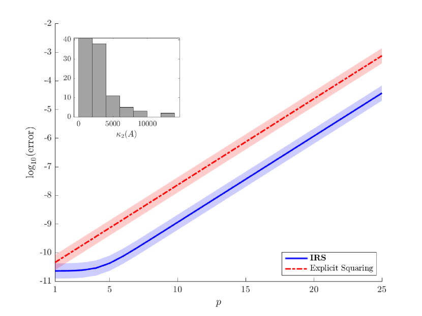
(a) Well-conditioned $A$.

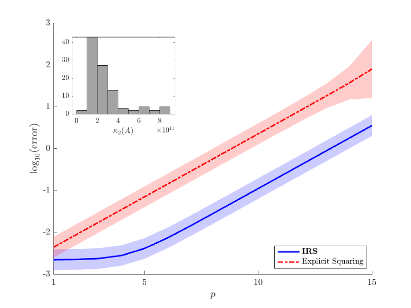
(b) Poorly-conditioned $A$

Figure 2: Log error for computing $(A^{-1}B)^{2^{p}}$ via IRS and explicit squaring when $A=B$. In (a) $A$ is a complex Gaussian while in (b) $A$ is a complex Gaussian modified to be close to singular. 100 trials (i.e., 100 draws of $A$) were used to produce both, with the average error for each algorithm plotted within a band whose width is twice the standard deviation of the population errors (computed via the unbiased $N-1$ estimator). For reference, we also include a histogram of the condition number of the input matrix $A$. Fewer steps of squaring are applied when $A$ is ill-conditioned to avoid exploding error at large $p$.

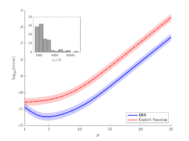
(a) Eigenvalues on $|z|=1$; $A$ well-conditioned.

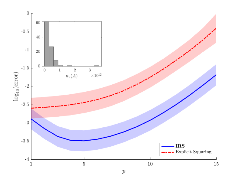
(b) Eigenvalues on $|z|=1$; $A$ poorly-conditioned.

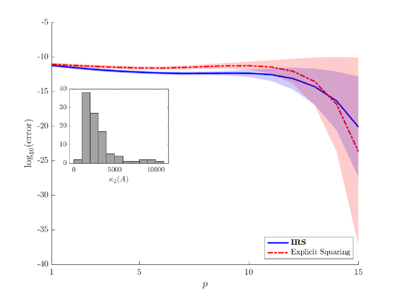
(c) Eigenvalues in $|z|\leq 1$; $A$ well-conditioned.

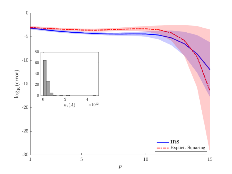
(d) Eigenvalues in $|z|\leq 1$; $A$ poorly-conditioned.

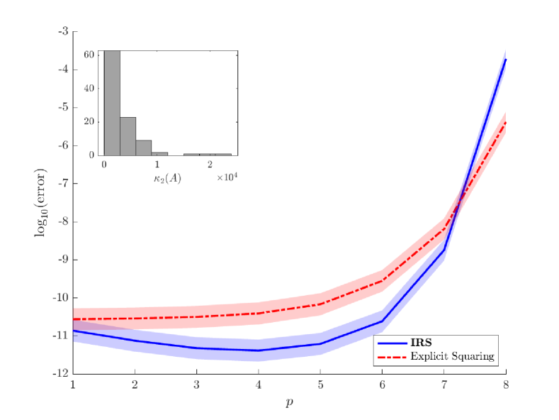
(e) Eigenvalues initially in $0.95\leq|z|\leq 1.05$; $A$ well-conditioned.

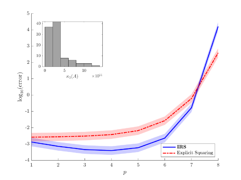
(f) Eigenvalues initially in $0.95\leq|z|\leq 1.05$; $A$ poorly-conditioned.

Figure 3: A repeat of Figure 2, this time with $B=AVDV^{H}$ for $V$ Haar and $D$ diagonal. In plots (a) and (b) the diagonal entries of $D$ (equivalently the eigenvalues of $A^{-1}B$) are sampled from the unit circle, in (c) and (d) they are sampled from the unit disk, while in (e) and (f) they are sampled from the annulus $0.95\leq|z|\leq 1.05$. Here, we cut off squaring when error begins to explode ((b), (e), and (f)) or becomes negligible ((c) and (d)) .

We start with the toy example $A=B$ (i.e., $D=I$). This is a nice initial test since $(A^{-1}B)^{2^{p}}=I$ is readily available (exactly) for any $p$. We consider a $1000\times 1000$ version of this problem in two regimes – one in which $A$ is a standard Gaussian and considered to be well-conditioned and another in which $A$ is drawn randomly and modified to ensure it is poorly-conditioned. Figure 2 plots average error in both squaring algorithms on this example for $100$ draws of $A$ (with both conditionings).
While these results look good – IRS outperforms naive, explicit squaring regardless of the conditioning of $A$ – we should be cautious given how structured the toy example is. With this in mind, we move next to general $C=VDV^{H}$, where the diagonal entries of $D$ are sampled from either the unit circle, unit disk, or the annulus $0.95\leq|z|\leq 1.05$. The latter allows us to test the situation where $A^{-1}B$ has eigenvalues outside the unit circle without having them blow up so quickly that computing even (4.0.1) becomes ill-conditioned.
Figure 3 reproduces Figure 2 for these more general problems, again with $n=1000$. When $A^{-1}B$ has eigenvalues on the unit circle or within the unit disk, we see roughly the same behavior as in the toy example: IRS outperforms explicit squaring whether or not $A$ is well-conditioned. When $A^{-1}B$ has eigenvalues in the annulus, on the other hand, IRS does better only to a certain point, after which its error outpaces the naive approach.
Intuitively, this should be tied to the conditioning of $A_{p}$. When $A^{-1}B$ has eigenvalues in the annulus $0.95\leq|z|\leq 1.05$ – and in particular outside of the unit circle – the corresponding pencil $(A,B)$ has an eigenvalue inside the unit disk, which translates to an eigenvalue near zero for $(A_{p},B_{p})$. It is not difficult to show

$$\sigma_{n}(A_{p})\leq|\lambda|||B_{p}||_{2}$$ (4.1.1)

for $\lambda$ any eigenvalue of $(A_{p},B_{p})$, which (recalling that $||B_{p}||_{2}$ grows by at most small constants) implies that $A_{p}$ is likely to become ill-conditioned for large values of $p$ in this setting. This is verified in Figure 4, which plots the evolution of $\kappa_{2}(A_{p})$ depending on the initial location of the eigenvalues of $A^{-1}B$. Interestingly, we observe a sort of regularization in these plots; regardless of the conditioning of $A$ or the location of eigenvalues of $A^{-1}B$, the first few steps of IRS appear to decrease the condition number of $A_{p}$. This is the likely explanation for the initial decrease in error in each plot of Figure 3.

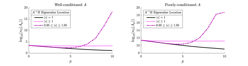
Figure 4: Evolution of $\kappa_{2}(A_{p})$ in IRS. In each case, $n=1000$ and $B=AVDV^{H}$, where $V$ is Haar unitary and $D$ is diagonal with nonzero entries sampled from the corresponding eigenvalue location. Each curve is the average of 50 trials, each using independently drawn $A$ and $V$.

4.2 Matrix Exponentials

We turn next to one of the applications discussed in Section 1 – the scaling and squaring method for evaluating matrix exponentials. Recall that this algorithm computes $e^{M}$ by selecting a value of $s$ and squaring a Padé approximation of $e^{M/2^{s}}$, which is itself a rational function of $M/2^{s}$. At its core, the method computes $(A^{-1}B)^{2^{s}}$ for $A$ and $B$ polynomials of the scaled matrix $M/2^{s}$.

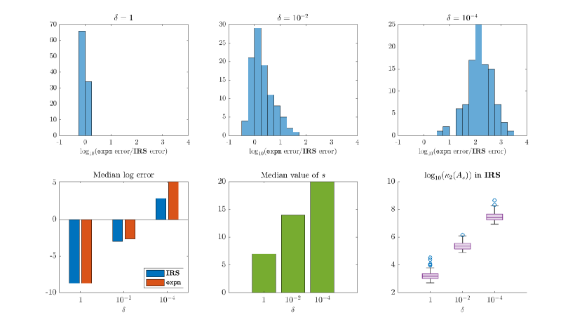
Figure 5: Performance data for standard scaling and squaring (i.e., expm) and an IRS-based alternative when used to compute a $1000\times 1000$ exponential $e^{M}$. In each case, $M=VDV^{-1}$ for $D$ a diagonal matrix (with nonzero entries samples from $|z|\leq 1$) and $V$ constructed according to (4.2.2). For each value of $\delta$, results are shown for 100 draws of $D$ and $V$. Error for both algorithms is measured as the spectral norm difference between the computed exponential and $Ve^{D}V^{-1}$. For each run, $s$ is the number of steps of squaring applied and $A_{s}$ is the output of IRS that must be inverted to compute the exponential.

Matlab implements scaling and squaring as the default for computing a dense matrix exponential via the intrinsic expm, meaning we can test a version of scaling and squaring that incorporates IRS by editing the source code of expm accordingly. For our purposes we change only the final squaring step; while we could explore how different choices of $s$ impact the accuracy of each method, we leave that to future work and instead consider $s$ to be more or less a black box.
Once again, we construct our examples via a diagonalization $M=VDV^{-1}$, in which case

$$A^{-1}B=e^{M/2^{s}}=Ve^{D/2^{s}}V^{-1}.$$ (4.2.1)

Here, $D$ has diagonal entries randomly sampled from the unit disk while $V$ is assembled by drawing a complex Gaussian $G$, computing a singular value decomposition $G=U\Sigma W^{H}$, and setting

$$V=G-(1-\delta)\sigma_{n}(G)uw^{H}$$ (4.2.2)

for $\delta\in\left\{1,10^{-2},10^{-4}\right\}$ and $u,w$ the last columns of $U$ and $W$ respectively. Changing the value of $\delta$ allows us to test problems with ever more ill-conditioned eigenvectors. As we will see, this corresponds to a larger value of $s$; in particular, we forgo the unitary $V$ from the previous examples since such problems often prompt expm to select $s=0$.
Before applying either version of scaling and squaring, we pause to note that, for this application, $A^{-1}B$ always fits squarely into the annulus example from the previous section. That is, the eigenvalues of $A^{-1}B$ are the diagonal entries of $e^{D/2^{s}}$, which are by construction only slightly larger than one in modulus. Unlike the general setting, however, we also know that squaring (which here functions to undo the initial scaling) cannot drive eigenvalues to be arbitrarily large. In particular, the eigenvalues of $(A^{-1}B)^{2^{s}}$ are bounded in modulus by the exponential of the spectral radius of $A^{-1}B$ (which in our case is one). Hence, we might hope that IRS can avoid the ill-conditioning observed in the previous section.
We now evaluate $e^{M}$ for all three values of $\delta$ using both versions of scaling and squaring. For each choice of $\delta$, Figure 5 presents data for both standard and IRS-based scaling and squaring with $100$ draws of $V$ and $D$ and $n=1000$. Here, error is measured as $||e^{M}-Ve^{D}V^{-1}||_{2}$, where $e^{M}$ stands in for the computed exponential (coming from either algorithm). We need to be a bit careful about how we interpret this error: $Ve^{D}V^{-1}$ may come with additional roundoff error itself, particularly as $V$ becomes more ill-conditioned, and moreover a certain loss of accuracy is attributable to the choice of the Padé approximation, which neither squaring approach may be able to overcome.
The first row of Figure 5 presents histograms of relative error for different values of $\delta$. We see here that IRS-based scaling and squaring reliably outperforms expm as the condition number of $V$ grows. Looking to the second row, this appears to be a consequence of the corresponding increase in $s$, and in particular the fact that the condition number of $A_{s}$ – the output of IRS that must eventually be inverted – stays relatively manageable, as we anticipated. Said another way, the lack of ill-conditioning of $A_{s}$ appears to allow IRS to better mitigate error growth when the number of squaring steps is large. While IRS is essentially equivalent to standard scaling and squaring when $\delta=1$ and neither version is particularly accurate when $\delta=10^{-4}$, we note a sweet spot around $\delta=10^{-2}$, where scaling and squaring is fairly accurate and IRS is capable of extending that to an extra digit or more.
The examples presented in this section should be taken as a proof of concept, indicating that IRS outperforms explicit squaring on certain problems, including the matrix exponential application considered here. While we might postulate that IRS is likely to do better when the eigenvalues of $(A^{-1}B)^{2^{p}}$ stay relatively small – either because the initial eigenvalues of $A^{-1}B$ belong to the unit disk or because the number of squaring steps is not too large – more testing is needed to obtain robust guidelines for its use.

5 Conclusion

In this paper, we have shown that an implicit algorithm for computing $(A^{-1}B)^{2^{p}}$ exhibits stability in finite arithmetic, both theoretically and empirically. Given these results, we make the case that IRS is deserving of further study outside the realm of divide-and-conquer eigensolvers. As demonstrated here, it has broader applicability than, and may outperform, a naive squaring algorithm at small additional arithmetic cost.
Future work could pursue improvements in the QR perturbation bound and the suboptimal forward error result presented in Appendix A. More generally we might ask, can the behavior in Figure 4 be codified theoretically?

6 Acknowledgements

This work was supported by Graduate Fellowships for STEM Diversity (GFSD) and NSF grant DMS 2154099. Special thanks to Anne Greenbaum for helpful correspondence and for suggesting the work of Bhatia used in Section 2. Thanks also to Ioana Dumitriu and James Demmel for guidance and feedback on earlier drafts of this paper.

Appendix A Comparison with Explicit Squaring

In this appendix, we compare IRS with the naive squaring algorithm in the setting where $(A^{-1}B)^{2^{p}}$ is needed explicitly (meaning the outputs $A_{p}$ and $B_{p}$ of IRS are not sufficient on their own). As in Section 3, the analysis here is presented in finite arithmetic. With this in mind, we introduce a third black-box algorithm to handle $n\times n$ matrix inversion. Note that a logarithmically stable inversion algorithm is necessitated here if we wish to continue working with fast matrix multiplication [11, Section 3].

Assumption A.1.

There exists a $(\mu_{\text{INV}}(n),c_{\text{INV}})$-stable matrix inversion algorithm $\textbf{INV}(\cdot)$ satisfying

$$||\textbf{INV}(A)-A^{-1}||_{2}\leq\kappa_{2}(A)^{c_{\text{INV}}\log(n)}\mu_{\text{INV}}(n){\bf u}||A^{-1}||_{2}$$ (A.0.1)

in $T_{\text{INV}}(n)$ operations.

Building off INV and 1.2, we can state Algorithm 2 – our finite-arithmetic, explicit algorithm for computing $(A^{-1}B)^{2^{p}}$.

Algorithm 2 Finite-Arithmetic Explicit Squaring (ES)
Input: $A,B\in{\mathbb{C}}^{n\times n}$ and $p$ a positive integer
Output: $(A^{-1}B)^{2^{p}}$

1:$C=\textbf{INV}(A)$

2:$D_{0}=\textbf{MM}(C,B)$

3:for $j=1:p$ do

4:     $D_{j}=\textbf{MM}(D_{j-1},D_{j-1})$

5:end for

6:return $D_{p}$

Our goal in this section is to explore situations where IRS (combined with a post-processing step that computes $A_{p}^{-1}B_{p}$) exhibits comparable or even better (theoretical) stability than ES, if there are any.

A.1 Flop Count

Before quantifying forward error, we do a quick flop count. $\textbf{ES}(A,B,p)$ requires only one matrix inversion and $p+1$ matrix multiplications, meaning it uses $T_{\text{INV}}(n)+(p+1)T_{\text{MM}}(n)$ arithmetic operations overall. IRS, on the other hand, requires $p(T_{\text{QR}}(n)+2T_{\text{MM}}(n))$ operations just to computes $A_{p}$ and $B_{p}$. Adding in the $T_{\text{INV}}(n)+T_{\text{MM}}(n)$ flops required to compute $A_{p}^{-1}B_{p}$ yields a final count of

$$T_{\text{INV}}(n)+pT_{\text{QR}}(n)+(2p+1)T_{\text{MM}}(n).$$ (A.1.1)

As expected, IRS requires significantly more arithmetic operations, a consequence of the costly block QR factorizations. We do note, however, that since our black-box assumptions accommodate fast matrix multiplication (see work of Demmel and collaborators [12, 11]) we can assume $T_{\text{QR}}(n)=O(T_{\text{MM}}(n))$ and $T_{\text{INV}}(n)=O(T_{\text{MM}}(n))$, meaning both algorithms have the same asymptotic flop count of $O(pT_{\text{MM}}(n))$.

A.2 Forward Error

We are now ready to bound forward error for IRS. We start with two intermediate results, the first of which concerns a simple, two step algorithm for computing $A^{-1}B$. We follow that with perturbation bounds for $A^{-1}B$ and $A^{2^{p}}$.

Lemma A.2.

Given $A,B\in{\mathbb{C}}^{n\times n}$, consider the two step, finite-arithmetic algorithm

1. $C={\textbf{INV}}(A)$

2. $D={\textbf{MM}}(C,B)$

where INV and MM satisfy A.1 and 1.2 respectively. Then

$$||D-A^{-1}B||_{2}\leq\left[\mu_{\text{MM}}(n){\bf u}+(1+\mu_{\text{MM}}(n){\bf u})\kappa_{2}(A)^{c_{\text{INV}}\log(n)}\mu_{\text{INV}}(n){\bf u}\right]||A^{-1}||_{2}||B||_{2}.$$

Proof.

We start by expanding $||D-A^{-1}B||_{2}$ as

$$||D-A^{-1}B||_{2}=||D-CB+CB-A^{-1}B||_{2}\leq||D-CB||_{2}+||C-A^{-1}||_{2}||B||_{2}.$$ (A.2.1)

Applying (1.3.4) and (A.0.1), this becomes

$$||D-A^{-1}B||_{2}\leq\mu_{\text{MM}}(n){\bf u}||C||_{2}||B||_{2}+\kappa_{2}(A)^{c_{\text{INV}}\log(n)}\mu_{\text{INV}}(n){\bf u}||A^{-1}||_{2}||B||_{2}.$$ (A.2.2)

We obtain the final inequality by simplifying with $||C||_{2}\leq||A^{-1}||_{2}+\kappa_{2}(A)^{c_{\text{INV}\log(n)}}\mu_{\text{INV}}(n){\bf u}||A^{-1}||_{2}$. ∎

Lemma A.3.

Suppose $A,B,\tilde{A},\tilde{B}\in{\mathbb{C}}^{n\times n}$ satisfy $||A-\tilde{A}||_{2},||B-\tilde{B}||_{2}\leq\delta$. Then,

$$||A^{-1}B-\tilde{A}^{-1}\tilde{B}||_{2}\leq\delta||A^{-1}||_{2}\left(\frac{\sigma_{n}(A)+||B||_{2}}{\sigma_{n}(A)-\delta}\right).$$

Proof.

We first observe

$$||A^{-1}B-\tilde{A}^{-1}\tilde{B}||_{2} =||A^{-1}B-A^{-1}\tilde{B}+A^{-1}\tilde{B}-\tilde{A}^{-1}\tilde{B}||_{2}$$ (A.2.3)

$$\leq||A^{-1}||_{2}||B-\tilde{B}||_{2}+||A^{-1}-\tilde{A}^{-1}||\tilde{B}||_{2}$$

$$\leq\delta||A^{-1}||_{2}+||A^{-1}(\tilde{A}-A)\tilde{A}^{-1}||_{2}||\tilde{B}||_{2}$$

$$\leq\delta||A^{-1}||_{2}(1+||\tilde{A}^{-1}||_{2}||\tilde{B}||_{2}).$$

Since 2.3 implies

$$||\tilde{A}^{-1}||_{2}=\frac{1}{\sigma_{n}(\tilde{A})}\leq\frac{1}{\sigma_{n}(A)-\delta}$$ (A.2.4)

and similarly $||\tilde{B}||_{2}\leq||B||_{2}+\delta$, we obtain

$$||A^{-1}B-\tilde{A}^{-1}\tilde{B}||_{2}\leq\delta||A^{-1}||_{2}\left(1+\frac{||B||_{2}+\delta}{\sigma_{n}(A)-\delta}\right),$$ (A.2.5)

which is equivalent to the listed inequality. ∎

Lemma A.4.

Suppose $A,\tilde{A}\in{\mathbb{C}}^{n\times n}$ satisfy $||A-\tilde{A}||_{2}\leq\delta$. Then for any integer $p\geq 1$

$$||A^{2^{p}}-\tilde{A}^{2^{p}}||_{2}\leq\delta\prod_{j=1}^{p}\left(||A||_{2}^{2^{j-1}}+(||A||_{2}+\delta)^{2^{j-1}}\right).$$

Proof.

This follows inductively from

$$||A^{2^{p}}-\tilde{A}^{2^{p}}||_{2} =||A^{2^{p}}-A^{2^{p-1}}\tilde{A}^{2^{p-1}}+A^{2^{p-1}}\tilde{A}^{2^{p-1}}-\tilde{A}^{2^{p}}||_{2}$$ (A.2.6)

$$\leq||A^{2^{p-1}}(A^{2^{p-1}}-\tilde{A}^{2^{p-1}})||_{2}+||(A^{2^{p-1}}-\tilde{A}^{2^{p-1}})\tilde{A}^{2^{p-1}}||_{2}$$

$$\leq||A^{2^{p-1}}-\tilde{A}^{2^{p-1}}||_{2}\left(||A||_{2}^{2^{p-1}}+||\tilde{A}||_{2}^{2^{p-1}}\right)$$

$$\leq||A^{2^{p-1}}-\tilde{A}^{2^{p-1}}||_{2}\left(||A||_{2}^{2^{p-1}}+(||A||_{2}+\delta)^{2^{p-1}}\right)$$

noting that the base case is $||A-\tilde{A}||_{2}\leq\delta$. ∎

With these lemmas, we can now extend 3.6 to bound the forward error in an IRS-based algorithm for computing $(A^{-1}B)^{2^{p}}$.

Theorem A.5.

For $\mu(n)=\max\left\{\mu_{\text{MM}}(n),\mu_{\text{QR}}(n),\mu_{\text{INV}}(n)\right\}$ let $\epsilon$ and ${\bf u}$ as in 3.6. Given $A,B\in{\mathbb{C}}^{n\times n}$ and $p\in{\mathbb{N}}_{+}$, suppose $(A^{-1}B)^{2^{p}}$ is computed according to the three-step algorithm

1. $[A_{p},B_{p}]={\textbf{IRS}}(A,B,p)$

2. $C={\textbf{INV}}(A_{p})$

3. $D={\textbf{MM}}(C,B_{p})$.

Then,

$$||D-(A^{-1}B)^{2^{p}}||_{2}\leq\mu(n){\bf u} \left[1+(1+\mu(n){\bf u})\kappa_{2}(A_{p})^{c_{\text{INV}}\log(n)}\right]||A_{p}^{-1}||_{2}||B_{p}||_{2}$$

$$+\epsilon\left|\left|\binom{A}{B}\right|\right|_{2}||A_{p}^{-1}||_{2}\left(\frac{\sigma_{n}(A_{p})+||B_{p}||_{2}}{\sigma_{n}(A_{p})-\epsilon||\binom{A}{B}||_{2}}\right)$$

$$+\delta\prod_{j=1}^{p}\left(||A^{-1}B||_{2}^{2^{j-1}}+(||A^{-1}B||_{2}+\delta)^{2^{j-1}}\right)$$

where $\delta=\mu(n){\bf u}||\binom{A}{B}||_{2}||A^{-1}||_{2}\left(\frac{\sigma_{n}(A)+||B||_{2}}{\sigma_{n}(A)-\mu(n){\bf u}||\binom{A}{B}||_{2}}\right)$.

Proof.

Set $\tau=\mu(n){\bf u}$ and let $\tilde{A},\tilde{B},\overline{A}_{p},\overline{B}_{p}\in{\mathbb{C}}^{n\times n}$ be the matrices guaranteed by 3.6, where $\overline{A}_{p}^{-1}\overline{B}_{p}=(\tilde{A}^{-1}\tilde{B})^{2^{p}}$ and $||A-\tilde{A}||_{2},||B-\tilde{B}||_{2}=\tau||\binom{A}{B}||_{2}$. Expanding $||D-(A^{-1}B)^{2^{p}}||_{2}$ as

$$||D-(A^{-1}B)^{2^{p}}||_{2} =||D-A_{p}^{-1}B_{p}+A_{p}^{-1}B_{p}-\overline{A}_{p}^{-1}\overline{B}_{p}+(\tilde{A}^{-1}\tilde{B})^{2^{p}}-(A^{-1}B)^{2^{p}}||_{2}$$ (A.2.7)

$$\leq||D-A_{p}^{-1}B_{p}||_{2}+||A_{p}^{-1}B_{p}-\overline{A}_{p}^{-1}\overline{B}_{p}||_{2}+||(\tilde{A}^{-1}\tilde{B})^{2^{p}}-(A^{-1}B)^{2^{p}}||_{2}$$

we bound each term individually. First, A.2 implies

$$||D-A_{p}^{-1}B_{p}||_{2}\leq\left[\tau+(1+\tau)\kappa_{2}(A_{p})^{c_{\text{INV}}\log(n)}\tau\right]||A_{p}^{-1}||_{2}||B_{p}||_{2}.$$ (A.2.8)

Next, 3.6 and A.3 combine to give

$$||A_{p}^{-1}B_{p}-\overline{A}_{p}^{-1}\overline{B}_{p}||_{2}\leq\epsilon\left|\left|\binom{A}{B}\right|\right|_{2}||A_{p}^{-1}||_{2}\left(\frac{\sigma_{n}(A_{p})+||B_{p}||_{2}}{\sigma_{n}(A_{p})-\epsilon||\binom{A}{B}||_{2}}\right)$$ (A.2.9)

and similarly

$$||\tilde{A}^{-1}\tilde{B}-A^{-1}B||_{2}\leq\tau\left|\left|\binom{A}{B}\right|\right|_{2}||A^{-1}||_{2}\left(\frac{\sigma_{n}(A)+||B||_{2}}{\sigma_{n}(A)-\tau||\binom{A}{B}||_{2}}\right)=\delta.$$ (A.2.10)

Applying A.4 then yields

$$||(\tilde{A}^{-1}\tilde{B})^{2^{p}}-(A^{-1}B)^{2^{p}}||_{2}\leq\delta\prod_{j=1}^{p}\left(||A^{-1}B||_{2}^{2^{j-1}}+(||A^{-1}B||_{2}+\delta)^{2^{j-1}}\right).$$ (A.2.11)

We obtain the final bound on $||D-(A^{-1}B)^{2^{p}}||_{2}$ by combining (A.2.8), (A.2.9), and (A.2.11). ∎

This result is not particularly useful because of its dependence on $A_{p}$, and in particular $||A_{p}^{-1}||_{2}$. While we know both $||A_{p}||_{2}$ and $||B_{p}||_{2}$ are at most a constant multiple of $||A||_{2}$ and $||B||_{2}$ respectively, we have no bound on $||A_{p}^{-1}||_{2}$. In fact, (4.1.1) implies that $||A_{p}^{-1}||_{2}$ is guaranteed to become arbitrarily large in some cases.
Nevertheless, we can still compare this result with error propagation in ES. To do this, let $\delta_{j}=||D_{j}-(A^{-1}B)^{2^{j}}||_{2}$ for $D_{j}$ the matrix obtained after $j$ steps of squaring in ES. Recalling $D_{j}=\textbf{MM}(D_{j-1},D_{j-1})$, it is not too hard to see

$$\delta_{j} =||D_{j}-(A^{-1}B)^{2^{j}}||_{2}$$ (A.2.12)

$$=||D_{j}-D_{j-1}^{2}+D_{j-1}^{2}-D_{j-1}(A^{-1}B)^{2^{j-1}}+D_{j-1}(A^{-1}B)^{2^{j-1}}-(A^{-1}B)^{2^{j}}||_{2}$$

$$\leq||D_{j}-D_{j-1}^{2}||_{2}+||D_{j-1}||_{2}||D_{j-1}-(A^{-1}B)^{2^{j-1}}||_{2}+||D_{j-1}-(A^{-1}B)^{2^{j-1}}||_{2}||(A^{-1}B)^{2^{j-1}}||_{2}$$

$$\leq\mu_{\text{MM}}(n){\bf u}||D_{j-1}||_{2}^{2}+\left(||D_{j-1}||_{2}+||(A^{-1}B)^{2^{j-1}}||_{2}\right)\delta_{j-1}.$$

Bounding $||D_{j-1}||_{2}$ by $||(A^{-1}B)^{2^{j-1}}||_{2}+\delta_{j-1}$ and rearranging, we conclude

$$\delta_{j}\leq\left[(1+\mu_{\text{MM}}(n){\bf u})\left(2||A^{-1}B||_{2}^{2^{j-1}}+\delta_{j-1}\right)\right]\delta_{j-1}+\mu_{\text{MM}}(n){\bf u}||A^{-1}B||_{2}^{2^{j}}.$$ (A.2.13)

This inequality allows us to bound error inductively, where the base case

$$\delta_{0}\leq\left[\mu_{\text{MM}}(n){\bf u}+(1+\mu_{\text{MM}}(n){\bf u})\kappa_{2}(A)^{c_{\text{INV}}\log(n)}\mu_{\text{INV}}(n){\bf u}\right]||A^{-1}||_{2}||B||_{2}$$ (A.2.14)

is given by A.2. Assuming a regime where $\delta_{j}<1$ and using $\mu(n)$ as in A.5, ES error can be roughly bounded as

$$\delta_{p}\leq O\left(\prod_{j=1}^{p}2(1+\mu(n){\bf u})||A^{-1}B||_{2}^{2^{j-1}}\right)\mu(n){\bf u}\left[1+(1+\mu(n){\bf u})\kappa_{2}(A)^{c_{\text{INV}}\log(n)}\right]||A^{-1}||_{2}||B||_{2}.$$ (A.2.15)

For fixed ${\bf u}$, this bound is likely to be looser than our corresponding result for IRS only if $\kappa_{2}(A_{p})$ is not too large, and in particular close to, or even smaller than, $\kappa_{2}(A)$. In this case, the third term in A.5 dominates and may come out ahead of (A.2.15) since $\delta$ depends only on $||A^{-1}||_{2}$ instead of $\kappa_{2}(A)^{\log(n)}$.
In Section 4, we saw that this was indeed the case for certain problems, though we have no way to guarantee when it occurs theoretically. It is possible that adding additional conditions to 1.3, for example that the main $n\times n$ blocks of $Q$ are all minimally well-conditioned, could allow us to bound $\kappa_{2}(A_{p})$ in terms of $\kappa_{2}(A)$ and therefore remove the dependence of A.5 on $A_{p}$. It is still an open question whether such a condition is viable at all

let alone available via some black-box algorithm compatible with fast matrix multiplication.

References

- [1] Awad H. Al-Mohy and Nicholas J. Higham. A new scaling and squaring algorithm for the matrix exponential. SIAM Journal on Matrix Analysis and Applications, 31(3):970–989, 2010.
- [2] Mario Arioli, B. Codenotti, and Claudia Fassino. The Padé method for computing the matrix exponential. Linear Algebra and its Applications, 240, 06 1996.
- [3] Zhaojun Bai, James Demmel, and Ming Gu. An inverse free parallel spectral divide and conquer algorithm for nonsymmetric eigenproblems. Numerische Mathematik, 76:279–308, 1997.
- [4] Grey Ballard, James Demmel, and Ioana Dumitriu. Minimizing communication for eigenproblems and the singular value decomposition. ArXiv, abs/1011.3077, 2010.
- [5] Grey Ballard, James Demmel, Ioana Dumitriu, and Alexander Rusciano. A generalized randomized rank-revealing factorization. ArXiv, abs/1909.06524, 2019.
- [6] Rajendra Bhatia. Pinching, trimming, truncating, and averaging of matrices. The American Mathematical Monthly, 107(7):602–608, 2000.
- [7] Rajendra Bhatia. Fourier Series. Classroom Resource Materials. Mathematical Association of America, 2005.
- [8] Rajendra Bhatia and Kalyan Mukherjea. Variation of the unitary part of a matrix. SIAM Journal on Matrix Analysis and Applications, 15(3):1007–1014, 1994.
- [9] A. Ya. Bulgakov and S.K. Godunov. Circular dichotomy of the spectrum of a matrix. Siberian Mathematical Journal, 29:734–744, 1988.
- [10] Don Coppersmith and Shmuel Winograd. Matrix multiplication via arithmetic progressions. Journal of Symbolic Computation, 9(3):251–280, 1990.
- [11] James Demmel, Ioana Dumitriu, and Olga Holtz. Fast linear algebra is stable. Numerische Mathematik, 108:59–91, Oct 2007.
- [12] James Demmel, Ioana Dumitriu, Olga Holtz, and Robert Kleinberg. Fast matrix multiplication is stable. Numerische Mathematik, 106, 04 2006.
- [13] James Demmel, Ioana Dumitriu, and Ryan Schneider. Generalized pseudospectral shattering and inverse-free matrix pencil diagonalization. ArXiv, abs/2306.03700, 2023.
- [14] Anne Greenbaum. Personal communication.
- [15] Nicholas J. Higham. Accuracy and Stability of Numerical Algorithms. Society for Industrial and Applied Mathematics, Second edition, 2002.
- [16] Nicholas J. Higham. The scaling and squaring method for the matrix exponential revisited. SIAM Review, 51(4):747–764, 2009.
- [17] Roger A. Horn and Charles R. Johnson. Matrix Analysis. Cambridge University Press, 2 edition, 2012.
- [18] Hanyu Li and Yimin Wei. Improved rigorous perturbation bounds for the LU and QR factorizations. Numerical Linear Algebra with Applications, 22(6):1115–1130, 2015.
- [19] A. N. Malyshev. Computing invariant subspaces of a regular linear pencil of matrices. Siberian Mathematical Journal, 30:559–567, 1989.
- [20] Alexander N. Malyshev. Parallel algorithm for solving some spectral problems of linear algebra. Linear Algebra and its Applications, 188-189:489–520, 1993.
- [21] Cleve Moler and Charles Van Loan. Nineteen dubious ways to compute the exponential of a matrix, twenty-five years later. SIAM Review, 45(1):3–49, 2003.
- [22] Petko H. Petkov. Componentwise perturbation analysis of the QR decomposition of a matrix. Mathematics, 10(24), 2022.
- [23] G. W. Stewart. Perturbation bounds for the QR factorization of a matrix. SIAM Journal on Numerical Analysis, 14(3):509–518, 1977.
- [24] G.W. Stewart and J. Sun. Matrix Perturbation Theory. Computer Science and Scientific Computing. Elsevier Science, 1990.
- [25] V. Strassen. Gaussian elimination is not optimal. Numerische Mathematik, 13:354–356, 1969.
- [26] Ji-Guang Sun. Perturbation bounds for the Cholesky and QR factorizations. BIT Numerical Mathematics, 31(2):341–352, jun 1991.
- [27] Ji-Guang Sun. On perturbation bounds for the QR factorization. Linear Algebra and its Applications, 215:95–111, 1995.
- [28] Virginia Vassilevska Williams. Multiplying matrices faster than coppersmith-winograd. In Proceedings of the Forty-Fourth Annual ACM Symposium on Theory of Computing, STOC ’12, page 887–898. Association for Computing Machinery, 2012.
- [29] Virginia Vassilevska Williams, Yinzhan Xu, Zixuan Xu, and Renfei Zhou. New bounds for matrix multiplication: from alpha to omega. ArXiv, abs/2307.07970, 2023.