Pólya urns on hypergraphs

Abstract.

We study Pólya urns on hypergraphs and prove that, when the incidence matrix of the hypergraph is injective, there exists a point $v=v(H)$ such that the random process converges to $v$ almost surely. We also provide a partial result when the incidence matrix is not injective.

1. Introduction

In 1923, George Pólya introduced a simple urn model that has attracted attention to probabilists. Nowadays called classical Pólya urn or simply Pólya urn, the simplicity of this random process with reinforcement allows for many variations and adaptations to more complicated settings, some of which model concrete situations in areas such as neuroscience, population dynamics, and social networks.

We are interested in Pólya urns on hypergraphs, as introduced in [BBCL15]. Consider a hypergraph $H=(G,E)$ with $V=[m]=\{1,2,\ldots,m\}$ and $|E|=N$, where every vertex $v\in G$ belongs to at least one hyperedge $I\in E$. Place a bin at each vertex, and assume that on vertex $i$ the bin contains initially $B_{i}(0)\geq 1$ balls. We consider the following random process of adding $N$ balls to the bins at each step: if the numbers of balls after step $n-1$ are $B_{1}(n-1),\ldots,B_{m}(n-1)$, step $n$ consists of adding, to each hyperedge $I\in E$, one ball to one of its vertices according to the following probability:

$${\mathbb{P}}\left[{i\text{ is chosen among }I\text{ at step }n}\right]=\dfrac{B_{i}(n-1)}{\sum\limits_{j\in I}B_{j}(n-1)}\,\cdot$$

We study the assymptotic behavior of the proportion of balls in the bins of $G$, as the number of steps grows. More specifically, let $N_{0}=\sum_{i=1}^{m}B_{i}(0)$ denote the initial total number of balls, let $x_{i}(n)=\tfrac{B_{i}(n)}{N_{0}+nN}$, $i\in[m]$, be the proportion of balls at vertex $i$ after step $n$, and let $x(n)=(x_{1}(n),\ldots,x_{m}(n))$. We characterize the limiting behavior of $x(n)$ using a combinatorial information of the hypergraph, given by its incidence matrix $I(H)$, see the definition in Section 1.1. Also, let $\Gamma=\{(x_{1},\ldots,x_{m})\in\mathbb{R}^{m}:x_{1}+\cdots+x_{m}=0\}$.

Theorem 1.1.

Let $H$ be a finite hypergraph. If the restriction of $I(H)$ to $\Gamma$ is injective, then there exists a point $v=v(H)$ such that $x(n)$ converges to $v$ almost surely.

This result is more general than the one stated in the abstract, since it only requires the restriction $I(H)\restriction_{\Gamma}$ to be injective. We also provide a partial answer when the restriction is not injective. Let $\Delta^{m-1}=\{(x_{1},\ldots,x_{m})\in\mathbb{R}^{m}:x_{i}\geq 0\text{ and }x_{1}+\cdots+x_{m}=1\}$ be the $(m-1)$–th dimensional simplex.

Theorem 1.2.

Let $H$ be a finite hypergraph. There exists a closed connected subset $\mathscr{J}=\mathscr{J}(H)$ of an affine subspace of $\mathbb{R}^{m}$ such that the limit set of $x(n)$ is contained in $\mathscr{J}$ almost surely. If the limit set of $x(n)$ does not intersect $\partial\Delta^{m-1}$ almost surely, then $x(n)$ converges to a point of $\mathscr{J}$ almost surely.

As a motivation for studying Pólya urns on hypergraphs, consider a market containing $m$ companies and $N$ products. Each product is sold by a subset of the companies. We can represent the market by an hypergraph $H=(V,E)$ where $V$ is the set of companies and each $I\in E$ represents a product. The companies try to use their size and reputation to boost their sales. Assuming that each client wants to buy one unit of each of the $N$ products at a moment, his/her choice of a company that sells the product $I$ corresponds to adding a ball to the respective company of the hyperedge $I$. Therefore, the Pólya urn on $H$ describes in broad strokes the long-term evolution of the market.

We can also enhance the model studied in [SP00], which considers a network of agents that play repeated games in pairings and then improve their skill by gaining experience. If the games are played by more than two agents according to an underlying hypergraph, then the experience of the agents can be represented by a Pólya urn on a hypergraph, where the numbers of balls in the bins represent the skill levels gained by the agents.

There are many recent variant and developments in the theory of Pólya urn schemes and related topics, see e.g. [ACG19, ACG20, SAG22, AMR16, BC22, CDPLM19, CH21, CJ22, HHK21, HHK23, vdHHKR16, KMS22, RPP22, Sah16]. Prior to its introduction in [BBCL15], Pemantle considered a Pólya urn model on $V=[m]$ with a single hyperedge $\{1,2,\ldots,m\}$, which is the same as a classical Pólya urn with balls of $m$ color [Pem92]. Up to this particular setting and to the authors’ knowledge, the present article gives the first general result for Pólya urns on hypergraphs.

For us, there are two reasons to study Pólya urns on hypergraphs. On the theoretical side, hypergraphs are more complex than graphs, hence their study introduces new technical difficulties and requires new ideas. On the practical side, it is possible to model a much larger class of situations with hypergraph-based interactions.

The case of Pólya urns on graphs introduced in [BBCL15] actually considers, for a fixed $\alpha>0$, the model of adding balls to the bins with probability proportional to the $\alpha$–th power of its current number of balls. Here, we only consider the case $\alpha=1$, which we call the linear case. For graphs, the limiting behavior in the linear case has been completely solved in the series of works [BBCL15, CL14, Lim16]. The final result is the following.

Theorem 1.3 ([BBCL15, CL14, Lim16]).

Let $G$ be a finite connected graph.

1. If $G$ is not balanced bipartite, then there is a point $v=v(G)$ such that $x(n)$ converges to $v$ almost surely.

2. If $G$ is balanced bipartite, then there is a closed interval $\mathfs J=\mathfs J(G)$ such that $x(n)$ converges to a point of $\mathfs J$ almost surely.

The proofs of Theorems 1.1 and 1.2 follow very closely the approach used to prove Theorem 1.3, which consists of writing $x(n)$ as a stochastic approximation algorithm, i.e. as a small perturbations of a vector field $F$, see Section 2. By the work of Benaïm [Ben96, Ben99], it is possible to relate the limiting behavior of $x(n)$ with dynamical properties of $F$.

One contribution of our work is to identify the combinatorial object that is related to the equilibria set of $F$, which is the incidence matrix of the hypergraph, see Section 1.1 for the definition. When restricted to $\Gamma$ (which is the tangent space of the simplex $\Delta^{m-1}$), this matrix provides the space of candidates for limits of $x(n)$, which is a subset $\mathfs J$ of an affine subspace of $\mathbb{R}^{m}$. We point out that our result applies, in particular, to Pólya urns on graphs, in which the role of the incidence matrix was not evident, and rather the adjacency matrix was used.

Another contribution of our work is to show that, for points in the interior of $\mathfs J$, the behavior of $F$ in the transverse direction to $\mathfs J$ is contractive, see Lemma 4.1. The proof of this fact for graphs was wrongly obtained in [Lim16], so we take the chance to correct this issue.

We believe that Theorem 1.2 can be improved to show that $x(n)$ converges almost surely, even when its limit set is contained in $\partial\Delta^{m-1}$ with positive probability. There are indeed cases when the limit set is contained in $\partial\Delta^{m-1}$ almost surely, see Section 5.

1.1. Notation

We consider a hypergraph $G=(V,E)$ where $V=[m]=\{1,2,\ldots,m\}$ and $|E|=N$. An element $I\in E$ is called an hyperedge. We assume that every $i\in[m]$ belongs to at least one hyperedge.

Simplex $\Delta^{m-1}$: We let

$$\Delta^{m-1}=\{(x_{1},\ldots,x_{m})\in\mathbb{R}^{m}:x_{i}\geq 0\text{ and }x_{1}+\cdots+x_{m}=1\}$$

denote the $(m-1)$–dimensional simplex, which is a manifold with boundary.

Tangent space $\Gamma$: We let

$$\Gamma=\{(x_{1},\ldots,x_{m})\in\mathbb{R}^{m}:x_{1}+\cdots+x_{m}=0\},$$

which is the tangent space of $\Delta^{m-1}$ at every $v\in{\rm int}(\Delta^{m-1})$.

Given a hyperedge $I\in E$ and $v\in\mathbb{R}^{m}$, we write

$$v_{I}:=\sum_{i\in I}v_{i}.$$

Recall that we start with $B_{1}(0),\ldots,B_{m}(0)\geq 1$ balls in the vertices $1,\ldots,m$ respectively, and that $N_{0}=\sum_{i=1}^{m}B_{i}(0)$ denotes the initial total number of balls. After $n$ steps, $B_{1}(n),\ldots,B_{m}(n)$ denote the number of balls in the vertices $1,\ldots,m$ respectively. The total number of balls after step $n$ is $N_{0}+nN=\sum_{i=1}^{m}B_{i}(n)$.

Incidence matrix $I(H)$: The incidence matrix of $H$ is the matrix $I(H)$ with dimensions $N\times m$, indexed by $E\times V$, whose entry $(I,i)$ is 1 if $i\in I$ and 0 otherwise.

Subspace $K$: We let $K={\rm ker}(I(H)\restriction_{\Gamma})$.

In the sequel, we fix a hypergraph $H$.

2. Stochastic approximation algorithms

Pólya urns on graphs are examples of stochastic approximation algorithms [BBCL15, §2]. In this section, we show that the same occurs to Pólya urns on hypergraphs.

Stochastic approximation algorithm: A stochastic approximation algorithm is a discrete time process $\{x(n)\}_{n\geq 0}\subset\mathbb{R}^{m}$ of the form

$$x(n+1)-x(n)=\gamma_{n}\left[F(x(n))+u_{n}\right]$$

where $\{\gamma_{n}\}_{n\geq 0}$ is a sequence of nonnegative scalars, $F:\mathbb{R}^{m}\to\mathbb{R}^{m}$ is a vector field, and $u_{n}\in\mathbb{R}^{m}$ is a random vector that depends on $x(n)$ only.

For simplicity, we just write $x(n)$ for the sequence $\{x(n)\}_{n\geq 0}$. Let $\mathfs F_{n}$ be the sigma-algebra generated by the process up to step $n$. Since $u_{n}$ only depends on $x(n)$ we can assume, after changing $F$, that ${\mathbb{E}}\left[{u_{n}}|{\mathfs F_{n}}\right]=0$. Recall that we are fixing a hypergraph $H$, and letting $x(n)$ denote the discrete process of Pólya urns on $H$.

Lemma 2.1.

The process $x(n)$ is a stochastic approximation algorithm.

Proof.

Consider a family of $0,1$–valued random variables $\{\delta_{I\to i}(n+1)\}_{I\in E,i\in I}$ such that:

1. If $I_{1}\neq I_{2}$, then $\delta_{I_{1}\to i_{1}}(n+1)$ and $\delta_{I_{2}\to i_{2}}(n+1)$ are independent for all $i_{1}\in I_{1},i_{2}\in I_{2}$;

2. $\sum_{i\in I}\delta_{I\to i}(n+1)=1$ for every $I\in E$;

3. ${\mathbb{E}}\left[{\delta_{I\to i}(n+1)}|{\mathscr{F}_{n}}\right]=\dfrac{x_{i}(n)}{x_{I}(n)}$ for every $i\in I$.

The random variable $\delta_{I\to i}(n+1)$ represents the addition or not, at step $n+1$, of the ball thrown at the hyperedge $I$ to the vertex $i$. Then $C_{i}(n+1)=\sum_{I\ni i}\delta_{I\to i}(n+1)$ is the number of balls added to the vertex $i$ at step $n+1$. Therefore

$$\ x_{i}(n+1)-x_{i}(n)=\frac{B_{i}(n)+C_{i}(n+1)}{N_{0}+(n+1)N}-\frac{B_{i}(n)}{N_{0}+nN}$$

$$=\frac{B_{i}(n)}{N_{0}+(n+1)N}\left(1-\frac{N_{0}+(n+1)N}{N_{0}+nN}\right)+\frac{C_{i}(n+1)}{N_{0}+(n+1)N}$$

$$=\frac{N}{N_{0}+(n+1)N}\left(-\frac{B_{i}(n)}{N_{0}+nN}\right)+\frac{C_{i}(n+1)}{N_{0}+(n+1)N}$$

$$=\frac{1}{\frac{N_{0}}{N}+(n+1)}\left(-x_{i}(n)+\frac{1}{N}C_{i}(n+1)\right).$$

Letting $\gamma_{n}=\frac{1}{\frac{N_{0}}{N}+(n+1)}$, $\xi_{i}(n)=\frac{1}{N}C_{i}(n+1)$ and $\xi(n)=(\xi_{1}(n),\ldots,\xi_{m}(n))$, we get that

$$x(n+1)-x(n)=\gamma_{n}(-x(n)+\xi(n)).$$

Hence $x(n)$ is a stochastic approximation algorithm. To finish the proof, we adjust $\xi(n)$ to have zero expectation. We have

$${\mathbb{E}}\left[{\xi_{i}(n)}|{\mathscr{F}_{n}}\right]=\mathbb{E}\left[\frac{1}{N}C_{i}(n+1)\Biggr{|}\mathscr{F}_{n}\right]=\frac{1}{N}\sum_{I\ni i}{\mathbb{E}}\left[{\delta_{I\to i}(n+1)}|{\mathscr{F}_{n}}\right]=\frac{1}{N}\sum_{I\ni i}\frac{x_{i}(n)}{x_{I}(n)}\,\cdot$$

Defining the vector field $F=(F_{1},\ldots,F_{m})$ by $F_{i}(v)=-v_{i}+\frac{1}{N}\sum\limits_{I\ni i}\frac{v_{i}}{v_{I}}$ and the vector $u_{n}=\xi(n)-{\mathbb{E}}\left[{\xi(n)}|{\mathscr{F}_{n}}\right]$, we obtain that

$$x(n+1)-x(n)=\gamma_{n}\left[F(x(n))+u_{n}\right],$$

with ${\mathbb{E}}\left[{u_{n}}|{\mathfs F_{n}}\right]=0$. This concludes the proof. ∎

Since $F$ involves fractions which can have zero denominator, we now give its proper definition. Fix $c<\tfrac{1}{N}$.

Set $\Delta$: We let $\Delta=\{x_{1},\ldots,x_{m})\in\Delta^{m-1}:x_{I}\geq c,\forall I\in E\}$.

Vector field $F$: We define $F=(F_{1},\ldots,F_{m}):\Delta\to\mathbb{R}^{m}$ where

$$F_{i}(v)=-v_{i}+\frac{1}{N}\sum_{I\ni i}\frac{v_{i}}{v_{I}}\,\cdot$$

Note that $F(v)\in\Gamma$ for every $v\in\Delta$ and that $F$ is Lipschitz. Now we prove that $F$ defines a semiflow. For that, we consider the ODE

$$\frac{dv(t)}{dt}=F(v(t))$$

and prove that $\Delta$ is positively invariant under this ODE (we will also say that $\Delta$ is positively invariant under $F$). Given $I\in E$, we have

$$\frac{dv_{I}}{dt}=\sum_{i\in I}F_{i}(v)=\sum_{i\in I}\left(-v_{i}+\frac{1}{N}\sum_{J\ni i}\frac{v_{i}}{v_{J}}\right)\geq-v_{I}+\frac{1}{N}\sum_{i\in I}\frac{v_{i}}{v_{I}}=-v_{I}+\frac{1}{N}\,\cdot$$

If $v\in\partial\Delta$ with $v_{I}=c$, then

$$\frac{dv_{I}}{dt}=-c+\frac{1}{N}>0$$

and so $F$ points inwards $\Delta$ at its boundary.

2.1. The vector field $F$ is gradient-like

Now we prove that $F$ is gradient-like. The proof is similar to the one for Pólya urns on graphs [BBCL15, Lemma 4.1]. Let us recall some definitions.

Equilibria set: A point $v\in\Delta$ is called an equilibrium for $F$ if $F(v)=0$. The equilibria set of $F$ is denoted by $\Lambda=\{v\in\Delta:v\text{ is an equilibrium}\}$.

Lyapunov function: A continuous map $L:\Delta\to\mathbb{R}$ is called a Lyapunov function for $F$ if it is strictly monotone along any integral curve of $F$ outside of $\Lambda$. In this case, we call $F$ gradient-like.

Let $L:\Delta\rightarrow\mathbb{R}$ be the function

$$L(v_{1},\dots,v_{m})=-\sum_{i=1}^{m}v_{i}+\frac{1}{N}\sum_{I\in E}\log v_{I}.$$

This is the version for hypergraphs of the Lyapunov function used for Pólya urns on graphs in [BBCL15]. The next lemma is the version for hypergraphs of [BBCL15, Lemma 4.1].

Lemma 2.2.

The function $L$ is a Lyapunov function for $F$. Therefore, $F$ is gradient-like.

Proof.

By direct calculation,

$$\frac{\partial L}{\partial v_{i}}=-1+\frac{1}{N}\sum_{I\ni i}\frac{1}{v_{I}}$$ (2.1)

and so

$$\frac{dv_{i}}{dt}=F_{i}(v(t))=v_{i}\left(-1+\frac{1}{N}\sum_{I\ni i}\frac{1}{v_{I}}\right)=v_{i}\frac{\partial L}{\partial v_{i}}\,\cdot$$

If $v=(v_{1}(t),\dots,v_{m}(t))$, $t\geq 0$, is an integral curve of $F$, then

$$\frac{d}{dt}(L\circ v)=\sum_{i=1}^{m}\frac{\partial L}{\partial v_{i}}\frac{dv_{i}}{dt}=\sum_{i=1}^{m}v_{i}\left(\frac{\partial L}{\partial v_{i}}\right)^{2}\geq 0.$$

The equality occurs if and only if $v_{i}\left(\frac{\partial L}{\partial v_{i}}\right)^{2}=0$ for all $i\in[m]$. This holds if and only if $F(v)=0$, hence $L$ is a Lyapunov function for $F$. ∎

2.2. Relation between $x(n)$ and $F$

In the sequel, we state a result of Benaïm that allows to relate asymptotic properties of $x(n)$ with dynamical properties of $F$. The theorem is not stated in its whole generality, but instead specialized to our situation.

Theorem 2.3 ([Ben96, Ben99]).

Let $F:\mathbb{R}^{m}\to\mathbb{R}^{m}$ be a gradient-like continuous vector field with unique integral curves, let $\Lambda$ be its equilibria set, let $L$ be a strict Lyapunov function, and let $x(n)$ be a solution to the recursion

$$x(n+1)-x(n)=\gamma_{n}[F(x(n))+u_{n}],$$

where $\gamma_{n}$ is a decreasing sequence satisfying $\lim\limits_{n\to\infty}\gamma_{n}=0$ and $\sum\limits_{n\geq 0}\gamma_{n}=\infty$, and $u_{n}\in\mathbb{R}^{m}$. Assume that:

1. the sequence $x(n)$ is bounded,
   

2. for each $T>0$,

   $$\lim_{n\to\infty}\left(\sup_{\{k:0\leq\tau_{k}-\tau_{n}\leq T\}}\left\lVert\sum_{i=n}^{k-1}\gamma_{i}u_{i}\right\rVert\right)=0,$$

   where $\tau_{n}=\sum\limits_{i=0}^{n-1}\gamma_{i}$, and

3. $L(\Lambda)\subset\mathbb{R}$ has empty interior.

Then the limit set of $x(n)$ is a connected subset of $\Lambda$.

Above, the $u_{n}$’s are fixed. Not every realization of the Pólya urn on hypergraphs satisfies the above conditions, but it does almost surely, as we will show in the next proposition. First, we need some notation.

Faces of $\Delta$: For each $S\subset[m]$, we let

$$\Delta_{S}=\{v\in\Delta:v_{i}=0\text{ iff }i\notin S\}$$

denote the face of $\Delta$ determined by $S$. Each $\Delta_{S}$ is a manifold with corners, positively invariant under $F$.

$S$–singularity for $L$: We call $v\in\Delta_{S}$ an $S$–singularity for $L$ or simply $S$–singularity if

$$\dfrac{\partial L}{\partial v_{i}}(v)=0\text{ for all }i\in S.$$

Let $\Lambda_{S}$ denote the set of $S-$singularities. Clearly, $\Lambda=\bigcup\limits_{S\subset[m]}\Lambda_{S}$.

Proposition 2.4.

Let $x(n)$ be the random process of Pólya urn on $H$. Then the limit set of $x(n)$ is a connected subset of $\Lambda$ almost surely.

Proof.

The sequence $\gamma_{n}=\frac{1}{\frac{N_{0}}{N}+(n+1)}$ is decreasing with $\lim\limits_{n\to\infty}\gamma_{n}=0$ and $\sum\limits_{n\geq 0}\gamma_{n}=\infty$. Note that $x(n)$ is bounded and so (1) always holds. We show that (2) holds almost surely. For each $n\geq 0$, let

$$M_{n}=\sum_{i=0}^{n-1}\gamma_{i}u_{i}.$$

The sequence of random variables $\{M_{n}\}_{n\geq 0}$ is a martingale adapted to the filtration $\{\mathscr{F}_{n}\}_{n\geq 0}$:

$${\mathbb{E}}\left[{M_{n+1}}|{\mathscr{F}_{n}}\right]=\sum_{i=0}^{n-1}\gamma_{i}u_{i}+{\mathbb{E}}\left[{\gamma_{n}u_{n}}|{\mathscr{F}_{n}}\right]=\sum_{i=0}^{n-1}\gamma_{i}u_{i}=M_{n}.$$

Furthermore, since $|u_{n}|\leq 1$, we have

$$\sum_{i=0}^{n}{\mathbb{E}}\left[{\|M_{i+1}-M_{i}\|^{2}}|{\mathfs F_{i}}\right]\leq\sum_{i=0}^{n}\gamma_{i}^{2}\leq\sum_{i\geq 0}\gamma_{i}^{2}<\infty.$$

This latter estimate implies that $\{M_{n}\}_{n\geq 0}$ converges almost surely to a finite random vector, see e.g. [Dur10, Theorem 5.4.9]. In particular, $\{M_{n}\}_{n\geq 0}$ is a Cauchy sequence almost surely, and so condition (2) holds almost surely.

It remains to check condition (3). Let $S\subset[m]$. The restriction $L\restriction_{\Delta_{S}}$ is a $C^{\infty}$ function, thus by the Sard theorem $L(\Lambda_{S})$ has zero Lebesgue measure. This implies that $L(\Lambda)=\bigcup\limits_{S\subset[m]}L(\Lambda_{S})$ has zero Lebesgue measure as well. In particular, it has empty interior. ∎

We note that $L$ is a (not necessarily strictly) concave function, hence so is its restriction $L\restriction_{\Delta_{S}}$. This implies that $\Lambda_{S}$ is equal to the set of global maxima of $L\restriction_{\Delta_{S}}$.

3. Unstable and non-unstable equilibria

In this section, we restrict the possible limits of $x(n)$. The idea, following [Pem92], is very similar to the one developed in [BBCL15], and consists of showing that there is zero probability of converging to an unstable equilibrium (we will define this notion shortly). The sole difference is that, contrary to the referred works, here we can have an uncountable number of unstable equilibria. Recall that $K={\rm ker}(I(H)\restriction_{\Gamma})$. The next lemma characterizes $\Lambda_{S}$, when it is non-empty.

Lemma 3.1.

Let $S\subset[m]$ and assume that $\Lambda_{S}\neq\emptyset$. For every $v\in\Lambda_{S}$, it holds that

$$\Lambda_{S}=\Delta_{S}\cap(v+K)=\{v+w\in\Delta_{S}:w\in K\}.$$

In other words, $\Lambda_{S}$ is the part of the affine subspace $v+K$ that intersects $\Delta_{S}$. Therefore, $\Lambda$ is contained in a finite union of translates of $K$.

Proof.

Fix $v\in\Lambda_{S}$ and let $w\in\Delta_{S}\cap(v+K)$. Since $v-w\in K$, we have $v_{I}=w_{I}$ for all $I\in E$, and so $\frac{\partial L}{\partial v_{i}}(w)=\frac{\partial L}{\partial v_{i}}(v)=0$ for every $i\in S$. Therefore, $w\in\Lambda_{S}$.

Conversely, let $w\in\Lambda_{S}$. Since $L\restriction_{\Delta_{S}}$ attains its global maxima in every point of $\Lambda_{S}$, we get $L(w)=L(v)$. Now, by the strict concavity of the logarithm, necessarily $w_{I}=v_{I}$ for all $I\in E$, and so $v-w\in K$. ∎

Now we analyze the dynamical type of equilibria.

3.1. Unstable equilibria

Let $S\subset[m]$, and fix $w\in\Lambda_{S}$. Consider the derivative $DF(w):T_{w}\Delta\to T_{w}\Delta$. In coordinates $v_{1},\ldots,v_{m}$, this linear transformation is represented by $JF(w)=\left(\frac{\partial F_{i}}{\partial v_{j}}\right)_{i,j}$ with:

$$\frac{\partial F_{i}}{\partial v_{j}}=\left\{\begin{array}[]{ll}w_{i}\dfrac{\partial^{2}L}{\partial v_{i}\partial v_{j}}&\text{if }i\not=j,\\ &\\ \dfrac{\partial L}{\partial v_{i}}+w_{i}\dfrac{\partial^{2}L}{\partial v_{i}^{2}}&\text{if }i=j.\\ \end{array}\right.$$ (3.1)

Without loss of generality, assuming that $S=\{k+1,\ldots,m\}$, we have that

$$JF(w)=\left[\begin{array}[]{cc}A&0\\ C&B\\ \end{array}\right]$$ (3.4)

where $A$ is a $k\times k$ diagonal matrix with diagonal entries $a_{ii}=\frac{\partial L}{\partial v_{i}}(w)$, $i\in[k]$. The spectrum of $JF(w)$ is equal to the union of the spectra of $A$ and $B$. Introducing the inner product $(x,y)=\sum_{i=k+1}^{m}x_{i}y_{i}/w_{i}$, we have $(Bx,y)=\langle Dx,y\rangle$, where $D$ is the Hessian matrix of $L$ restricted to the coordinates $v_{k+1},\ldots,v_{m}$ and $\langle\cdot,\cdot\rangle$ is the canonical inner product. Since $D$ is symmetric, $B$ is self-adjoint. Since $L$ is concave, $B$ is negative semidefinite. Therefore, the eigenvalues of $B$ are real and nonpositive, and so $JF(w)$ has a real positive eigenvalue if and only if $a_{ii}>0$ for some $i\in[k]$, which justifies the following definition.

Unstable equilibrium: We call $w\in\Lambda$ an unstable equilibrium if there exists $i\in[m]$ such that $w_{i}=0$ and $\frac{\partial L}{\partial v_{i}}(w)>0$. If $w$ is not unstable, we call $w$ a non-unstable equilibrium.

By definition, every equilibrium in the interior of $\Delta$ is non-unstable. The next lemma, proved in the Appendix, is the version for hypergraphs of [BBCL15, Lemma 5.2]. We let $L\{x(n)\}$ denote the limit set of $\{x(n):n\geq 0\}$.

Lemma 3.2.

Let $H$ be a finite hypergraph. If $v\in\Lambda$ is an unstable equilibrium, then

$$\mathds{P}\left[L\{x(n)\}\cap(v+K)\neq\emptyset\right]=0.$$

In particular, $\mathds{P}\left[\lim x(n)=v\right]=0$.

This formulation will be particularly important in the proof of Theorem 1.2.

3.2. Non-unstable equilibria and Lyapunov functions

The existence of non-unstable equilibria provides extra information on the behavior of $F$. This is the content of the next lemma, which is a version for hypergraphs of [CL14, Lemmas 3.1 and 3.2]. Given $w\in\Delta_{S}$ and $\chi\in(0,\min_{i\in S}w_{i}]$, let $\Delta^{w,\chi}=\{v\in\mathbb{R}^{n}:v_{i}\geq\chi,\forall i\in S\}$. Given $U\subset\Delta^{w,\chi}$, call $P:\Delta^{w,\chi}\to\mathbb{R}$ a Lyapunov function for $U$ if it is strictly monotone along the integral curves of $F$ outside $U$.

Lemma 3.3.

Let $w$ be a non-unstable equilibrium. There exists a set $J=J(w,\chi)\subset w+K$ such that $P:\Delta^{w,\chi}\to\mathbb{R}$ given by $P(v)=\sum_{i=0}^{m}w_{i}\log v_{i}$ is a Lyapunov function for $J$. In particular, $L\{x(n)\}\subset J$ almost surely.

Proof.

Inside $\Delta^{w,\chi}$ the function $P$ is differentiable, with

$$\frac{d}{dt}(P\circ v)=\sum_{i\in S}w_{i}\frac{1}{v_{i}}\frac{dv_{i}}{dt}=\sum_{i\in S}w_{i}\frac{\partial L}{\partial v_{i}}=\sum_{i=1}^{m}w_{i}\frac{\partial L}{\partial v_{i}}=-1+\frac{1}{N}\sum_{I\in E}\frac{w_{I}}{v_{I}}\,\cdot$$

Let $f:\Delta^{w,\chi}\to\mathbb{R}$ be given by $f(v)=-1+\frac{1}{N}\sum\limits_{I\in E}\frac{w_{I}}{v_{I}}$. Observe that $f(w)=0$. We will show that $f(v)\geq 0$, with equality if and only if $v\in J$ (to be defined below).

Step 1: $f$ is convex.

Since $x>0\mapsto\frac{1}{x}$ is convex, each $v\in\Delta^{w,\chi}\mapsto\frac{w_{I}}{v_{I}}$ is convex, thus $f$ is the sum of convex functions.

Step 2: $w$ is a global minimum of $f$.

Since $f$ is convex, it is enough to prove that $w$ is a local minimum of $f$. Let $v=w+(\varepsilon_{1},\ldots,\varepsilon_{m})$ with $\varepsilon_{1},\ldots,\varepsilon_{m}$ small enough. Of course, $\varepsilon_{i}\geq 0$ for $i\not\in S$. Applying the inequality $\frac{x}{x+\varepsilon}-1\geq-\frac{\varepsilon}{x}$ for $x,x+\varepsilon>0$, we have

$$\ f(v)-f(w)=\frac{1}{N}\sum_{I\in E}\left[\frac{w_{I}}{v_{I}}-1\right]\geq\frac{1}{N}\sum_{I\in E}-\frac{\varepsilon_{I}}{w_{I}}=-\sum_{i=1}^{m}\varepsilon_{i}\frac{1}{N}\sum_{I\ni i}\frac{1}{w_{I}}$$

$$=-\sum_{i=1}^{m}\varepsilon_{i}\left[1+\frac{\partial L}{\partial v_{i}}(w)\right]=-\sum_{i=1}^{m}\varepsilon_{i}\frac{\partial L}{\partial v_{i}}(w)\geq 0,$$

since $\varepsilon_{i}\frac{\partial L}{\partial v_{i}}(w)=0$ for $i\in S$, and $\varepsilon_{i}\frac{\partial L}{\partial v_{i}}(w)\leq 0$ for $i\not\in S$. Hence $w$ is a local minimum of $f$.

Step 3: The set of global minima of $f$ is $J=J(w,\chi):=\Delta^{w,\chi}\cap(w+K)$.

The set of global minima of a convex function is convex. Thus if $v\in\Delta^{w,\chi}$ with $f(v)=f(w)$, then $f(tv+(1-t)w)=tf(v)+(1-t)f(w)$ for all $t\in[0,1]$. Because $x>0\mapsto\frac{1}{x}$ is strictly convex, we get $v_{I}=w_{I}$ for all $I\in E$, and so $v-w\in K$. This shows that the set of global minima of $f$ is contained in $J$. Conversely, if $v\in J$, then $v_{I}=w_{I}$ for all $I\in E$, and so $f(v)=0$, which proves the reverse inclusion. ∎

4. Proof of Theorems 1.1 and 1.2

In this section, we prove the main theorems.

4.1. Proof of Theorem 1.1

The proof of this theorem is very similar to the proofs in [BBCL15, CL14, Lim16]. We start observing that, since $K=\{0\}$, each $\Lambda_{S}$ is either empty or a singleton. By Theorem 2.3, we conclude that $\lim x(n)\in\Lambda$ is a singleton almost surely. By Lemma 3.2, there is at least one non-unstable equilibrium $w\in\Lambda$. By Lemma 3.3, there is at most one non-unstable equilibrium. Therefore, $w$ is the only non-unstable equilibrium, and so $\lim x(n)=w$ almost surely.

4.2. Proof of Theorem 1.2

If $K=\{0\}$, then Theorem 1.1 provides the stronger result, hence we assume that $K\neq\{0\}$. By Lemma 3.2, there is at least one non-unstable equilibrium $w\in\Lambda$.

The set $\mathfs J$: We define $\mathfs J=\Delta^{m-1}\cap(w+K)$.

Clearly, $\mathfs J\subset\Lambda$ and every $v\in\mathfs J$ is non-unstable. We claim that $\mathfs J$ is the set of non-unstable equilibria. By contradiction, assume that there is $v\in\Lambda\backslash\mathfs J$ non-unstable. Then $(v+K)\cap(w+K)=\emptyset$. By Lemma 3.3, $L\{x(n)\}$ is contained in both $v+K$ and $w+K$ almost surely, a contradiction. Thus $\mathfs J$ is the set of non-unstable equilibria. Again by Lemma 3.2, $L\{x(n)\}$ is contained in $\mathfs J$ almost surely. This proves the first part of Theorem 1.2.

Now we prove the second part. Assume that $L\{x(n)\}\subset\Delta_{[m]}$ almost surely. This implies that $\Lambda_{[m]}\neq\emptyset$, so we can take $w$ above belonging to $\Lambda_{[m]}$. In particular, $\Lambda_{[m]}\subset\mathfs J$. We will show that $x(n)$ converges to a point of $\Lambda_{[m]}$ almost surely. We begin calculating the dynamical nature of $F$ transversely to $\Lambda_{[m]}$. Let $k={\rm dim}(K)$. Given $v\in\Lambda_{[m]}$, recall that $DF(v):T_{v}\Delta\to T_{v}\Delta$ has non-positive eigenvalues, due to the concavity of the Lyapunov function $L$.

Lemma 4.1.

For every $v\in\Lambda_{[m]}$, the derivative $DF(v)$ has $m-1-k$ negative eigenvalues, and 0 is an eigenvalue with multiplicity $k$.

Proof.

Consider the jacobian matrix $JF(v)$. We claim that ${\rm ker}(JF(v))={\rm ker}(I(H))$. This will conclude the proof, since it implies that ${\rm ker}(DF(v))=K$, which has dimension $k$ and $DF(v)$ has non-positive eigenvalues. The vector field $F$ is zero on $v+{\rm ker}(I(H))$, thus ${\rm ker}(I(H))\subset{\rm ker}(JF(v))$, so it is enough to prove that $I(H)$ and $JF(v)$ have the same rank.

Since $v\in\Delta_{[m]}$, we have $\frac{\partial L}{\partial v_{i}}(v)=0$ for all $i\in[m]$. From equation (3.1), $JF(v)=\left(v_{i}\frac{\partial^{2}L}{\partial v_{i}\partial v_{j}}(v)\right)_{i,j}$. Letting $B={\rm Hess}(L(v))$, this implies that $JF(v)=DB$ where $D$ is an invertible diagonal matrix with entries $v_{1},\ldots,v_{n}$, thus ${\rm rank}(JF(v))={\rm rank}(DB)={\rm rank}(B)$. We now relate $B$ with $I(H)$. By equality (2.1),

$$\frac{\partial L}{\partial v_{i}}=-1+\frac{1}{N}\sum_{I\ni i}\frac{1}{v_{I}}\ \ \Longrightarrow\ \ \frac{\partial^{2}L}{\partial v_{i}\partial v_{j}}=-\frac{1}{N}\sum_{I\ni i,j}\frac{1}{(v_{I})^{2}}\,\cdot$$

Let $E$ be the matrix $I(H)$ with the line relative to the hyperedge $I$ multiplied by $\tfrac{1}{v_{I}}$. Then ${\rm rank}(E)={\rm rank}(I(H))$ and the $(i,j)$–th entry of $E^{t}E$ is exactly $\sum_{I\ni i,j}\frac{1}{(v_{I})^{2}}$. Therefore $B=-\frac{1}{N}E^{t}E$, so that ${\rm rank}(B)={\rm rank}(E^{t}E)={\rm rank}(E)={\rm rank}(I(H))$. The conclusion is that ${\rm rank}(JF(v))={\rm rank}(I(H))$, which proves the lemma. ∎

Remark 4.2.

We take the chance to use Lemma 4.1 to correct a mistake in [Lim16], where one of the authors claims that, for Pólya urns on graphs, a result similar to Lemma 4.1 holds simply because the restriction $L\restriction_{\Delta_{[m]}}$ is concave and $\Lambda_{[m]}$ is the set of global maxima of this restriction. These conditions are not enough to ensure that no other zero eingevalue appears.

We are now in position to prove that $x(n)$ converges to a point of $\Lambda_{[m]}$ almost surely. The idea is to use the arguments of [CL14], which we will recast the main ideas. First, we introduce some notation. Let $\{\Phi_{t}\}_{t\geq 0}$ be the semiflow induced by $F$ and $\tau_{n}=\sum_{i=0}^{n}\gamma_{i}$. Let $\{X(t)\}_{t\geq 0}$ be the interpolation of $\{x(n)\}_{n\geq 0}$, defined by $X(\tau_{n})=x(n)$ and $X\restriction_{[\tau_{n},\tau_{n+1}]}$ linear, and let $d$ be the euclidean distance on $\Delta^{m-1}$.

Theorem 4.3 ([Ben99]).

Almost surely, the interpolated process satisfies

$$\sup_{T>0}\limsup_{t\to+\infty}\frac{1}{t}\log\left(\sup_{0\leq h\leq T}d\big{(}X(t+h),\Phi_{h}(X(t))\big{)}\right)\leq-\frac{1}{2}\,\cdot$$

For Pólya urns on graphs, this result is stated in [CL14, Lemma 4.1]. The proof for hypergraphs is the same, following from shadowing techniques that relate the rate of convergence of the interpolated process and the vector field, see [Ben99, Prop. 8.3]. The right-hand side of the inequality is the log-convergence rate $\frac{1}{2}\limsup\frac{\log\gamma_{n}}{\tau_{n}}=-\frac{1}{2}$.

We wish to show that $x(n)$ converges to a point of $\Lambda_{[m]}$ almost surely. It is enough to prove that the interpolated process $X(t)$ satisfies this property. Consider a foliation $\{\mathfs F_{x}\}_{x\in\Lambda_{[m]}}$ such that:

1. $\mathfs F_{x}$ is a submanifold with $\mathfs F_{x}\pitchfork\Lambda_{[m]}$ at the single point $x$.

2. $x$ is a hyperbolic attractor for $F\restriction_{\mathfs F_{x}}$. The speed of convergence depends on the negative eigenvalues of $DF(x)$.

The existence of this foliation follows from the theory of invariant manifolds for normally hyperbolic sets, see e.g. [HPS77, Theorem 4.1]. The leaves $\mathfs F_{x}$ depend smoothly on $x$. We let $\pi$ be the projection map such that $\pi\restriction_{\mathfs F_{x}}\equiv x$.

Fix one realization of the process $x(n)$ whose limit set does not intersect $\partial\Delta^{m-1}$ (by assumption, this holds almost surely). Then the limit set of $X(t)$ also does not intersect $\partial\Delta^{m-1}$, and so $X(t)$ has an accumulation point $y\in\Lambda_{[m]}$. Fix a compact neighborhood $V\subset\Lambda_{[m]}$ of $y$, and let $U\subset\Delta$ be a neighborhood of $V$. Taking $U$ small enough, the projection $\pi$ is 2–Lipschitz:

$$d(\pi(x),\pi(y))\leq 2d(x,y),\forall\,x,y\in U.$$ (4.1)

Fix a small parameter $\varepsilon>0$ and reduce $U$, if needed, so that

$$U=\{x\in\Delta:\pi(x)\in V\text{ and }d(x,\pi(x))<\varepsilon\}.$$ (4.2)

Let $a=\max\{\lambda:\lambda\not=0\text{ is eigenvalue of }DF(x),x\in V\}$. By Lemma 4.1, we have $a<0$, thus there is $C>0$ such that

$$d(\Phi_{t}(x),\pi(x))\leq Ce^{at}d(x,\pi(x)),\forall\,x\in U,\forall\,t\geq 0.$$

Lemma 4.4.

Assume that $X(t)\in U$. If $t,T$ are large enough, then

1. $d(\pi(X(t+T)),\pi(X(t)))<2e^{-\frac{t}{4}}$.

2. $X(t+T)\in U$.

Proof.

Same as [CL14, Lemma 4.4], using Theorem 4.3 and estimates (4.1), (4.2). ∎

Now, we repeat ipsis literis the arguments of [CL14], see also [Lim16], which consists of:

1. Fix large $t,T$, and let $X_{k}=X(t+kT)$, $k\geq 0$. Applying Lemma 4.4, prove that $\pi(X_{k})$ converges, say $\lim\pi(X_{k})=\widetilde{x}\in V$.

2. Prove that $\lim d(X_{k},\pi(X_{k}))=0$, hence $\lim X_{k}=\widetilde{x}$.

3. Prove that $X(t)$ also converges to $\widetilde{x}$.

Therefore $x(n)$ converges to $\widetilde{x}$. Since $V\subset\Lambda_{[m]}$, the proof of Theorem 1.2 is complete.

5. Examples and concluding remarks

Every solid $S$ can be viewed as an hypergraph $H$, whose hyperedges are the faces of $S$. For example, a tetrahedron is a hypergrah with $V=\{1,2,3,4\}$ and hyperedges $E=\{\{1,2,3\},\{1,2,4\},\{1,3,4\},\{2,3,4\}\}$. For the platonic solids, the kernel of $I(H)$ coincides with $K$, and their dimensions are:

Platonic solid	$\dim K$
Tetrahedron	$0$
Cube	4
Octahedron	2
Icosahedron	$0$
Dodecahedron	8

In all cases, the uniform measure $\left(\tfrac{1}{m},\ldots,\tfrac{1}{m}\right)$ is a non-unstable equilibrium. In particular, for the tetrahedron and the icosahedron the process $x(n)$ converges to the uniform measure almost surely.

As mentioned in the Introduction, we believe in the following conjecture.

Conjecture: For any finite hypergraph, $x(n)$ converges almost surely.

We are currently not able to prove this due to the behavior of $DF$ at $\partial\Delta^{m-1}$. As shown in Lemma 4.1, in the interior of the simplex the eigenvalues associated to directions transverse to $K$ are negative, but as we approach $\partial\Delta^{m-1}$ these eigenvalues can approach zero. Even worse: in $\partial\Delta^{m-1}$ the rank of $DF$ can decrease, thus creating zero eigenvalues in directions transverse to $K$. For example, consider the Pólya urn in the cube, with the following enumeration of vertices:

We have $\mathfs J=\Delta^{7}\cap(w+K)$, where $w=\left(\tfrac{1}{8},\ldots,\tfrac{1}{8}\right)$ and $K$ has dimension 4. On $w+K$, we have $v_{I}=\tfrac{1}{2}$ for all $I\in E$, hence

$$\tfrac{\partial^{2}L}{\partial v_{i}\partial v_{j}}=-\tfrac{1}{6}\tfrac{1}{\left(\tfrac{1}{2}\right)^{2}}\#\{I\in E:i,j\in I\}=-\tfrac{2}{3}\#\{I\in E:i,j\in I\}\,\cdot$$

The set $\mathfs J$ has points with different behavior for $F$:

1. For $v=\left(0,\tfrac{1}{4},0,\tfrac{1}{4},\tfrac{1}{8},\tfrac{1}{8},\tfrac{1}{8},\tfrac{1}{8}\right)$, the matrix

   $$JF(v)=-\tfrac{1}{12}\begin{bmatrix}0&0&0&0&0&0&0&0\\ 4&6&4&2&2&4&2&0\\ 0&0&0&0&0&0&0&0\\ 4&2&4&6&2&0&2&4\\ 2&1&0&1&3&2&1&2\\ 1&2&1&0&2&3&2&1\\ 0&1&2&1&1&2&3&2\\ 1&0&1&2&2&1&2&3\\ \end{bmatrix}$$

   has rank 4, hence no new eingevectors of 0 are created.

2. For $v=\left(\tfrac{1}{4},0,0,\tfrac{1}{4},0,\tfrac{1}{4},\tfrac{1}{4},0\right)$, the matrix

   $$JF(v)=-\tfrac{1}{6}\begin{bmatrix}3&2&1&2&2&1&0&1\\ 0&0&0&0&0&0&0&0\\ 0&0&0&0&0&0&0&0\\ 2&1&2&3&1&0&1&2\\ 0&0&0&0&0&0&0&0\\ 1&2&1&0&2&3&2&1\\ 0&1&2&1&1&2&3&2\\ 0&0&0&0&0&0&0&0\\ \end{bmatrix}$$

   has rank 3, and five eigenvectors of 0 in $\Gamma$. Hence, a new eingevalue 0 was created.

We believe that in this case, the limiting distribution is fully supported on $\mathfs J$ and depends on the initial condition $x(0)$. See the simulations in Figure 1 below, each consisting of 10000 iterations. The resulting points $\{(n,x(n)):0\leq n\leq 10000\}$ are plotted as a graph. Notice that, as $B_{1}(0)$ grows, $\lim x_{1}(n)$ tends to dominate the other limits.

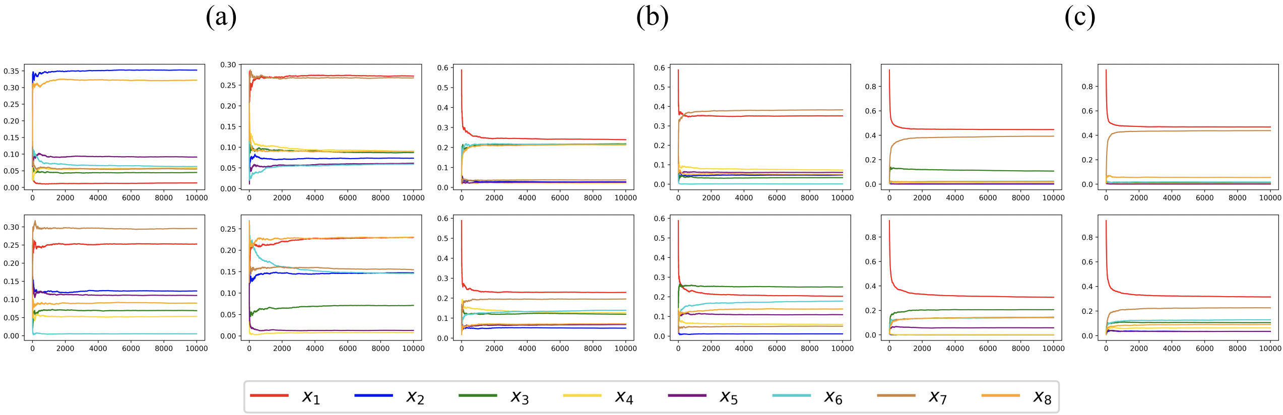
Figure 1. (a) Four simulations on the cube with initial condition $(1,1,1,1,1,1,1,1)$. (b) Four simulations on the cube with initial condition $(10,1,1,1,1,1,1,1)$. (c) Four simulations on the cube with initial condition $(100,1,1,1,1,1,1,1)$. The almost vertical components in the graphs in the first iterations are due to large oscillations in the beginning of the process.

Certainly, the hypothesis of Theorem 1.2 are not global, as the next lemma shows. Given a vertex $i\in[m]$, we let $E^{i}=\{I\in E:i\in I\}$ denote the set of hyperedges containing $i$.

Lemma 5.1.

Assume that there are $I\in E$ and $i,j\in I$ such that $E^{i}=\{I\}$ and $|E^{j}|>1$. If $w\in\Lambda$ with $w_{i}>0$, then $w$ is unstable. In particular, the limit set of $x(n)$ converges to $\partial\Delta^{m-1}$ almost surely.

Proof.

Since $w_{i}>0$, we have $\frac{\partial L}{\partial v_{i}}(w)=0$, then

$$0=\frac{\partial L}{\partial v_{i}}(w)=-1+\frac{1}{N}\cdot\frac{1}{w_{I}}\ \ \Longrightarrow\ \ w_{I}=\frac{1}{N}\,\cdot$$

Now,

$$\frac{\partial L}{\partial v_{j}}(w)=-1+\frac{1}{N}\left(\frac{1}{w_{I}}+\sum_{\begin{subarray}{c}J\ni j\atop{J\neq I}\end{subarray}}\frac{1}{w_{J}}\right)=\frac{1}{N}\sum_{J\ni j\atop{J\neq I}}\frac{1}{w_{J}}>0.$$

Since $w_{j}\frac{\partial L}{\partial v_{j}}(w)=0$, we have $w_{j}=0$, thus proving that $w$ is unstable. Therefore, every non-unstable equilibrium $w\in\Lambda$ must satisfy $w_{i}=0$. Applying Lemma 3.2, the proof is complete. ∎

This shows that there is a large class of hypergraphs that require a finer analysis of equilibria in $\partial\Delta^{m-1}$.

6. Acknowledgements

This work started during the undergraduate research program “Jornadas de Pesquisa para Graduação”, held at ICMC-USP in January 2023, which was partially supported by Centro de Ciências Matemáticas Aplicadas à Industria (CeMEAI - CEPID) under FAPESP Grant #2013/07375-0. The authors are grateful to Ali Tahzibi, Gracyella Salcedo, Guilherme Silva, Marcelo Tabarelli and Rafael Zorzetto for the discussions and support. MB was supported by CAPES and CNPq. YL was supported by CNPq and Instituto Serrapilheira, grant “Jangada Dinâmica: Impulsionando Sistemas Dinâmicos na Região Nordeste”.

Appendix A Non-convergence to unstable equilibria

In this appendix we prove Lemma 3.2, with methods similar to [BBCL15, Lemma 5.2]. Recall that $E^{i}=\{I\in E:i\in I\}$ is the set of hyperedges containing $i$.

Lemma A.1.

Let $v\in\Lambda$ with $v_{1}=0$ and $\tfrac{\partial L}{\partial v_{i}(v)}>3\delta$. Then there exists a neighborhood $\mathcal{N}$ of $v+K$ not containing any other equilibrium, an element $u\in\mathcal{N}$ and $\epsilon_{0}>0$ such that

1. $\frac{\partial L}{\partial v_{i}}(u)>3\delta+\frac{|E^{1}|\epsilon_{0}}{N}$, and

2. for all $w\in\mathcal{N}$ and $I\in E^{1}$ it holds

   $$\frac{1}{w_{I}}>\frac{1}{u_{I}}-\epsilon_{0}.$$

Proof.

Fix $\epsilon_{0}\in\left(0,\left(\frac{\partial L}{\partial v_{i}}(v)-3\delta\right)\frac{N}{|E^{1}|}\right)$, then $\frac{\partial L}{\partial v_{i}}(v)>3\delta+\frac{|E^{1}|\epsilon_{0}}{N}$. Since $\frac{\partial L}{\partial v_{i}}$ is continuous and equal to $\frac{\partial L}{\partial v_{i}}(v)$ along $v+K$, there exists a neighborhood $\mathcal{N}$ of $v+K$ small enough such that it does not contain any other equilibrium and also satisfies condition (1).

Given $I\in E^{1}$, the function $w\in\overline{\mathcal{N}}\mapsto\frac{1}{w_{I}}$ is uniformly continuous and therefore there exists $\overline{\delta}_{I}$ such that

$$|w-\widetilde{w}|<\overline{\delta}_{I}\implies\left|\frac{1}{w_{I}}-\frac{1}{\widetilde{w}_{I}}\right|<\epsilon_{0},\ \forall w,\widetilde{w}\in\overline{\mathcal{N}}.$$

Thus, if we take $\operatorname{diam}(\mathcal{N})<\max\limits_{I\in E^{1}}\overline{\delta}_{I}$, then condition (2) is also satisfied. ∎

Proof of Lemma 3.2.

Since $v$ is an unstable equilibrium, there exists $i\in[m]$ such that $v_{i}=0$ and $\frac{\partial L}{\partial v_{i}}(v)>0$. Without loss of generality, assume $i=1$. Since $L\{x(n)\}$ is a connected subset of $\Lambda$ (Theorem 2.3), if $v\in L\{x(n)\}$, then $L\{x(n)\}\subset v+K$. Firstly, we claim that

$$\mathds{P}\left[\lim\limits_{n\to\infty}B_{1}(n)=\infty\right]=1.$$ (A.1)

Fix an edge $I\in E^{1}$ and let $Z_{n}$ be the event that the vertex 1 is the chosen from hyperedge $I$ at step $n+1$. Because $1\leq B_{i}(n)\leq N_{0}+nN$ for all $i\in[m]$,

$$\mathds{P}\left[Z_{n}|Z_{k}^{\mathsf{c}},\ldots,Z_{n-1}^{\mathsf{c}}\right]\geq\dfrac{1}{|I|(N_{0}+nN)}$$

for every $k<n$. Then (A.1) follows by an adaptation of the Borel-Cantelli lemma.

Let $\delta>0$ and $\mathcal{N}$ be as in Lemma A.1, and fix $B$ large enough (to be specified later). We define the event $\mathcal{Y}_{n}=\{x(k)\in\mathcal{N},\forall k\geq n\}\cap\{B_{1}(n)\geq B\}$. Observing that $\{L\{x(n)\}\subset v+K\}\subset\bigcup_{m\geq n}\mathcal{Y}_{m}$ for every $n>0$, it is enough to prove that there is $n_{0}>0$ such that

$$\mathds{P}\left[\mathcal{Y}_{n}\right]=0,\ \forall n>n_{0}.$$

Let $\mathcal{G}_{n}=\mathcal{F}_{n}\cap\mathcal{Y}_{n}$. Define $c=\frac{\delta(1+2\delta)}{1+\frac{3}{2}\delta}>0$. We claim that, if $B$ is large enough, then there exists $n_{0}>0$ such that

$$\mathds{E}\left[\log x_{1}((1+\delta)n)|\mathcal{G}_{n}\right]\geq\log x_{1}(n)+\frac{1}{2}\log(1+c),\ \forall n>n_{0}.$$ (A.2)

Once we have this, suppose there exists $n>n_{0}$ such that $\mathds{P}[\mathcal{Y}_{n}]>0$ and define $T_{k}=(1+\delta)^{k}n$ and $X_{k}=\log x_{1}(T_{k})$. By (A.2),

$$\mathds{E}\left[X_{k+1}|\mathcal{G}_{n}\right]=\mathds{E}\left[\mathds{E}\left[X_{k+1}|\mathcal{G}_{T_{k}}\right]|\mathcal{G}_{n}\right]\geq\mathds{E}\left[X_{k}|\mathcal{G}_{n}\right]+\frac{1}{2}\log(1+c)$$

and so by induction

$$\mathds{E}\left[X_{k}|\mathcal{G}_{n}\right]\geq\mathds{E}[X_{0}|\mathcal{G}_{n}]+\frac{k}{2}\log(1+c)\geq-\log\left(N_{0}+nN\right)+\frac{k}{2}\log(1+c).$$

Since the left hand side is nonpositive, we obtain a contradiction when $k$ is large enough.

Now we prove (A.2). Let $t\in\{n+1,\ldots,(1+\delta)n\}$. Restricted to $\mathcal{Y}_{n_{0}}$, for every $I\in E^{1}$ we have

$$\ \mathds{P}[1\text{ is chosen in }I\text{ at step }t]=\dfrac{B_{1}(t-1)}{B_{I}(t-1)}\geq\dfrac{B_{1}(n)}{N_{0}+(t-1)N}\cdot\dfrac{1}{x_{I}(t-1)}$$

$$\geq\dfrac{B_{1}(n)}{N_{0}+(t-1)N}\left(\dfrac{1}{u_{I}}-\epsilon_{0}\right).$$

Define a family of independent Bernoulli random variables $\{E_{t,I}\}$, $t=n+1,\ldots,(1+\delta)n$, $I\in E^{1}$ such that

$$\mathds{P}[E_{t,I}=1]=\dfrac{B_{1}(n)}{N_{0}+(t-1)N}\left(\dfrac{1}{u_{I}}-\epsilon_{0}\right).$$

Now couple $\{E_{t,I}\}$ to our model as follows: if $E_{t,I}=1$, then $1$ is chosen in $I$ at step $t$. Then

$$\mathds{E}\left[\sum_{\begin{subarray}{c}n+1\leq t\leq(1+\delta)n\\ I\in E^{1}\end{subarray}}E_{t,I}\right]=\sum_{I\in E^{1}}\left(\sum_{t=n+1}^{(1+\delta)n}\dfrac{B_{1}(n)}{N_{0}+(t-1)N}\left(\dfrac{1}{u_{I}}-\epsilon_{0}\right)\right)$$

$$=B_{1}(n)\left[\sum_{I\in E^{1}}\left(\dfrac{1}{u_{I}}-\epsilon_{0}\right)\right]\left[\sum_{t=n+1}^{(1+\delta)n}\dfrac{1}{N_{0}+(t-1)N}\right]\geq B_{1}(n)(1+3\delta)\log\left(1+\dfrac{\delta nN}{N_{0}+nN}\right).$$

If $n_{0}$ is large enough (such that $\frac{n_{0}N}{N_{0}+n_{0}N}>\frac{1}{1+\frac{1}{2}\delta}$), we get

$$\mathds{E}\left[\sum_{\begin{subarray}{c}n+1\leq t\leq(1+\delta)n\\ I\in E^{1}\end{subarray}}E_{t,I}\right]\geq B_{1}(n)\dfrac{\delta(1+3\delta)}{1+\frac{3}{2}\delta}.$$

By Chernoff bounds, if $\epsilon_{1}>0$, then there is $B_{0}$ large enough such that

$$\mathds{P}\left[\sum_{\begin{subarray}{c}n+1\leq t\leq(1+\delta)n\\ I\in E^{1}\end{subarray}}E_{t,I}>B_{1}(n)\dfrac{\delta(1+2\delta)}{1+\frac{3}{2}\delta}\right]>1-\epsilon_{1}$$

for every $B_{1}(n)>B_{0}$. Whenever the previous event holds, the coupling gives us

$$B_{1}((1+\delta)n)-B_{1}(n)\geq\sum_{\begin{subarray}{c}n+1\leq t\leq(1+\delta)n\\ I\in E^{1}\end{subarray}}E_{t,I}>B_{1}(n)\dfrac{\delta(1+2\delta)}{1+\frac{3}{2}\delta},$$

thus, $\mathds{P}[x_{1}((1+\delta)n)>x_{1}(n)(1+c)|\mathscr{G}_{n}]>1-\epsilon_{1}$. Now, because $x_{1}((1+\delta)n)>\frac{x_{1}(n)}{1+\delta}$, we get

$$\mathds{E}[\log x_{1}((1+\delta)n)|\mathscr{G}_{n}]>(1-\epsilon_{1})\log(x_{1}(n)(1+c))+\epsilon_{1}\log\left(\dfrac{x_{1}(n)}{1+\delta}\right).$$

For large $B_{0}$, $\epsilon_{1}$ can be made small enough such that

$$\mathds{E}[\log x_{1}((1+\delta)n)|\mathscr{G}_{n}]>\log x_{1}(n)+\dfrac{1}{2}\log(1+c),$$

thus proving (A.2), and hence Lemma 3.2. ∎

References

- [ACG19] Giacomo Aletti, Irene Crimaldi, and Andrea Ghiglietti. Networks of reinforced stochastic processes: asymptotics for the empirical means. Bernoulli, 25(4B):3339–3378, 2019.
- [ACG20] Giacomo Aletti, Irene Crimaldi, and Andrea Ghiglietti. Interacting reinforced stochastic processes: statistical inference based on the weighted empirical means. Bernoulli, 26(2):1098–1138, 2020.
- [AMR16] Tonći Antunović, Elchanan Mossel, and Miklós Z. Rácz. Coexistence in preferential attachment networks. Combin. Probab. Comput., 25(6):797–822, 2016.
- [BBCL15] Michel Benaim, Itai Benjamini, Jun Chen, and Yuri Lima. A generalized Pólya’s urn with graph-based interactions. Random Structures & Algorithms, 46(4):614–634, 2015.
- [BC22] Jacopo Borga and Benedetta Cavalli. Quenched law of large numbers and quenched central limit theorem for multiplayer leagues with ergodic strengths. Ann. Appl. Probab., 32(6):4398–4425, 2022.
- [Ben96] Michel Benaim. A dynamical system approach to stochastic approximations. SIAM J. Control Optim., 34(2):437–472, 1996.
- [Ben99] Michel Benaïm. Dynamics of stochastic approximation algorithms. In Séminaire de Probabilités, XXXIII, volume 1709 of Lecture Notes in Math., pages 1–68. Springer, Berlin, 1999.
- [CDPLM19] Irene Crimaldi, Paolo Dai Pra, Pierre-Yves Louis, and Ida G. Minelli. Synchronization and functional central limit theorems for interacting reinforced random walks. Stochastic Process. Appl., 129(1):70–101, 2019.
- [CH21] Yannick Couzinié and Christian Hirsch. Weakly reinforced Pólya urns on countable networks. Electron. Commun. Probab., 26:Paper No. 35, 10, 2021.
- [CJ22] Marcelo Costa and Jonathan Jordan. Phase transitions in non-linear urns with interacting types. Bernoulli, 28(4):2546–2562, 2022.
- [CL14] Jun Chen and Cyrille Lucas. A generalized pólya’s urn with graph based interactions: convergence at linearity. Electronic Communications in Probability, 19:1–13, 2014.
- [Dur10] Rick Durrett. Probability: theory and examples, volume 31 of Cambridge Series in Statistical and Probabilistic Mathematics. Cambridge University Press, Cambridge, fourth edition, 2010.
- [HHK21] Christian Hirsch, Mark Holmes, and Victor Kleptsyn. Absence of WARM percolation in the very strong reinforcement regime. Ann. Appl. Probab., 31(1):199–217, 2021.
- [HHK23] Christian Hirsch, Mark Holmes, and Victor Kleptsyn. Infinite WARM graphs III: strong reinforcement regime. Nonlinearity, 36(6):3013–3042, 2023.
- [HPS77] M. W. Hirsch, C. C. Pugh, and M. Shub. Invariant manifolds. Lecture Notes in Mathematics, Vol. 583. Springer-Verlag, Berlin-New York, 1977.
- [KMS22] Daniel Kious, Cécile Mailler, and Bruno Schapira. The trace-reinforced ants process does not find shortest paths. J. Éc. polytech. Math., 9:505–536, 2022.
- [Lim16] Yuri Lima. Graph-based pólya’s urn: completion of the linear case. Stochastics and Dynamics, 16(02):1660007, 2016.
- [Pem92] Robin Pemantle. Vertex-reinforced random walk. Probab. Theory Related Fields, 92(1):117–136, 1992.
- [RPP22] Rafael A. Rosales, Fernando P. A. Prado, and Benito Pires. Vertex reinforced random walks with exponential interaction on complete graphs. Stochastic Process. Appl., 148:353–379, 2022.
- [SAG22] Somya Singh, Fady Alajaji, and Bahman Gharesifard. A finite memory interacting Pólya contagion network and its approximating dynamical systems. SIAM J. Control Optim., 60(2):S347–S369, 2022.
- [Sah16] Neeraja Sahasrabudhe. Synchronization and fluctuation theorems for interacting Friedman urns. J. Appl. Probab., 53(4):1221–1239, 2016.
- [SP00] B. Skyrms and R. Pemantle. A dynamic model of social network formation. Proceedings of the National Academy of Sciences of the United States of America, 97(16):9340–9346, 2000.
- [vdHHKR16] Remco van der Hofstad, Mark Holmes, Alexey Kuznetsov, and Wioletta Ruszel. Strongly reinforced Pólya urns with graph-based competition. Ann. Appl. Probab., 26(4):2494–2539, 2016.