Feedback-guided data synthesis for
imbalanced classification

Abstract

Current status quo in machine learning is to use static datasets of real images for training, which often come from long-tailed distributions. With the recent advances in generative models, researchers have started augmenting these static datasets with synthetic data, reporting moderate performance improvements on classification tasks. We hypothesize that these performance gains are limited by the lack of feedback from the classifier to the generative model, which would promote the usefulness of the generated samples to improve the classifier’s performance. In this work, we introduce a framework for augmenting static datasets with useful synthetic samples, which leverages one-shot feedback from the classifier to drive the sampling of the generative model. In order for the framework to be effective, we find that the samples must be close to the support of the real data of the task at hand, and be sufficiently diverse. We validate three feedback criteria on a long-tailed dataset (ImageNet-LT) as well as a group-imbalanced dataset (NICO++). On ImageNet-LT, we achieve state-of-the-art results, with over $4\%$ improvement on underrepresented classes while being twice efficient in terms of the number of generated synthetic samples. NICO++ also enjoys marked boosts of over $5\%$ in worst group accuracy. With these results, our framework paves the path towards effectively leveraging state-of-the-art text-to-image models as data sources that can be queried to improve downstream applications.

1 Introduction

In the recent year, we have witnessed unprecedented progress in image generative models (Ho et al., 2020; Nichol et al., 2022; Ramesh et al., 2021; Rombach et al., 2022; Ramesh et al., 2022; Saharia et al., 2022; Balaji et al., 2022; Kang et al., 2023). The photo-realistic results achieved by these models has propelled an arms race towards their widespread use in content creation applications, and as a byproduct, the research community has focused on developing models and techniques to improve image realism (Kang et al., 2023) and conditioning-generation consistency (Hu et al., 2023; Yarom et al., 2023; Xu et al., 2023). Yet, the potential for those models to become sources of data to train machine learning models is still under debate, raising intriguing questions about the qualities that the synthetic data must possess to be effective in training downstream representation learning models.

Several recent works have proposed using generative models as either data augmentation or sole source of data to train machine learning models (He et al., 2023; Sariyildiz et al., 2023; Shipard et al., 2023; Bansal & Grover, 2023; Dunlap et al., 2023; Gu et al., 2023; Astolfi et al., 2023; Tian et al., 2023), reporting moderate model performance gains. These works operate in a static scenario, where the models being trained do not provide any feedback to the synthetic data collection process that would ensure the usefulness of the generated samples. Instead, to achieve performance gains, the proposed approaches often rely on laborious ’prompt engineering’ (Gu et al., 2023) to promote synthetic data to be close to the support of the real data distribution on which the downstream representation learning model is to be deployed (Shin et al., 2023). Moreover, recent studies have highlighted the limited conditional diversity in the samples generated by state-of-the-art image generative models (Hall et al., 2023; Cho et al., 2022; Luccioni et al., 2023; Bianchi et al., 2022), which may hinder the promise of leveraging synthetic data at scale. From these perspectives, synthetic data still falls short of real data.

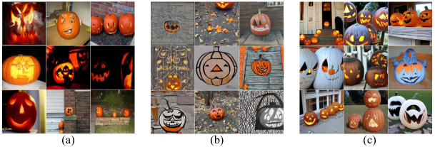
Figure 1: Exemplary samples from different distributions. Subfigures show random samples for Jack-o-lantern class coming from: (a) ImageNet-LT; (b) Latent Diffusion Model (LDM-unclip v2-1), conditioned on the text prompt Jack-o-lantern; (c) our pipeline.

Yet, the generative model literature has implicitly encouraged generating synthetic samples that are close to the support of the real data distribution by developing methods to increase the controllability of the generation process (Vendrow et al., 2023). For example, researchers have explored image generative models conditioned on images instead of only text (Casanova et al., 2021; Blattmann et al., 2022; Bordes et al., 2022). These approaches inherently offer more control over the generation process, by providing the models with rich information from a real image without relying on ’prompt engineering’ (Wei et al., 2022; Zhang et al., 2022; Lester et al., 2021). Similarly, the generative models literature has aimed to increase sample diversity by devising strategies to encourage models to sample from the tails of their distribution (Sehwag et al., 2022; Um & Ye, 2023). However, the promise of the above-described strategies to improve representation learning is yet to be shown.

In this work, we propose to leverage the recent advances in the generative models to address the shortcomings of synthetic data in representation learning, and introduce feedback from the downstream classifier model to guide the data generation process. In particular, we devise a framework which leverages a pre-trained image generative model to provide useful, and diverse synthetic samples that are close to the support of the real data distribution, to improve on representation learning tasks. Since real world data is most often characterized by long tail and open-ended distributions, we focus on imbalanced classification-scenarios, in which different classes or groups are unequally represented, to demonstrate the effectiveness of our framework. More precisely, we conduct experiments on ImageNet Long-Tailed (ImageNet-LT) (Liu et al., 2019) and NICO++ (Zhang et al., 2023) and show consistent performance gains w.r.t. prior art. Our contributions can be summarized as:

• We devise a diffusion model sampling strategy which leverages feedback from a pretrained classifier in order to generate samples that are useful to improve its own performance.

• We find that for the classifier’s feedback to be effective, the synthetic data must lie close to the support of the downstream task data distribution, and be sufficiently diverse.

• We report state-of-the-art results (1) on ImageNet-LT, with an improvement of $4\%$ on underrepresented classes while using half the amount of synthetic data than the previous state-of-the-art; and (2) on NICO++, with improvements of over $5\%$ in worst group accuracy.

Through experiments, we highlight how our proposed approach can be effectively implemented to enhance the utility of synthetic data. See Figure 1 for samples from our framework.

2 Background

Diffusion models.

Diffusion models (Sohl-Dickstein et al., 2015; Song & Ermon, 2019) learn data distributions $p({\bm{x}})$ or $p({\bm{x}}|y)$ by simulating the diffusion process in forward and reverse directions. In particular, Denoising Diffusion Probabilistic Models (DDPM) (Ho et al., 2020) add noise to data points in the forward process and remove it in the reverse process. The continuous-time reverse process in DDPM is given by, $\mathrm{d}\mathbf{x}_{t}=\left[\mathbf{f}(\mathbf{x}_{t},t)-g^{2}(t)\nabla\log{p^{t}(\mathbf{x}_{t})}\right]\mathrm{d}t+g(t)\mathrm{d}\mathbf{w}_{t},$ where $t$ indexes time, and $\mathbf{f}(\mathbf{x}_{t},t)$ and $g(t)$ are drift and volatility coefficients. A neural network $\epsilon_{\theta}^{(t)}({\bm{x}}_{t})$ is trained to predict noise in DDPM, aligning with the score function $\nabla\log{p^{t}(\mathbf{x}_{t})}$. Given a trained model $\epsilon_{\theta}^{(t)}({\bm{x}}_{t})$, Denoising Diffusion Implicit Models (DDIM) (Song et al., 2020), a more generic form of diffusion models, can generate an image ${\bm{x}}_{0}$ from pure noise ${\bm{x}}_{T}$ by repeatedly removing noise, getting ${\bm{x}}_{t-1}$ given ${\bm{x}}_{t}$ (from Song et al. (2020)):

$${\bm{x}}_{t-1} =\sqrt{\alpha_{t-1}}\underbrace{\left(\frac{{\bm{x}}_{t}-\sqrt{1-\alpha_{t}}\epsilon_{\theta}^{(t)}({\bm{x}}_{t})}{\sqrt{\alpha_{t}}}\right)}_{\text{`` predicted ${\bm{x}}_{0}$ ''}}+\underbrace{\sqrt{1-\alpha_{t-1}-\sigma_{t}^{2}}\cdot\epsilon_{\theta}^{(t)}({\bm{x}}_{t})}_{\text{``direction pointing to ${\bm{x}}_{t}$ ''}}+\underbrace{\sigma_{t}\epsilon_{t}}_{\text{random noise}},$$ (1)

with $\alpha_{t}$ and $\sigma_{t}$ as time-dependent coefficients and $\epsilon_{t}\sim{\mathcal{N}}({\bm{0}},{\bm{I}})$ being standard Gaussian noise.

Classifier-guidance in diffusion models.

Guidance in latent diffusion models involves leveraging additional information, such as class labels or text prompts, to condition the generated samples on. This modifies the score function as follows:

$$\nabla_{x}\log p_{\gamma}(x|y)=\nabla_{x}\log p(x)+\gamma\nabla_{x}\log p(y|x),$$ (2)

where $\gamma$ is a scaling factor. The term $\nabla_{x}\log p(y|x)$ is generally modeled either as classifier-guidance (Dhariwal & Nichol, 2021) or classifier-free guidance (Ho & Salimans, 2022). In the Latent Diffusion Model (LDM) used in this paper, $\nabla_{x}\log p(y|x)$ is modeled in a classifier-free approach and $\gamma$ controls its guidance strength.

3 Methodology

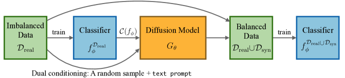
Figure 2: Overview of our framework. Given an imbalanced dataset, $\mathcal{D}_{\text{real}}$, a classifier $f_{\phi}(x)$ is initially trained. Knowing that the validation and test sets are balanced, the goal is to create a balanced training set using synthetic data. The Diffusion Model, $G_{\theta}$, is conditioned on a randomly selected real image and a label-containing text prompt. The model’s generation is also guided by feedback, $\mathcal{C}(f_{\phi})$, from the classifier to increase usefulness of the synthetic samples. Subsequently, $f_{\phi}(x)$ is retrained on the combined real and synthetic samples.

Figure 2 presents an overview of our proposed approach. We assume access to a pre-tained diffusion model, which takes as input an image and a text prompt, and produces an image consistent with the inputs. We train a classifier $f_{\phi}$ on an imbalanced dataset of real images, $\mathcal{D}_{\text{real}}$. This initial classifier serves as a foundation for the subsequent generation of synthetic samples. We then collect a dataset of synthetic data, $\mathcal{D}_{\text{syn}}$, by conditioning the pre-trained diffusion model on text prompts formatted as class-label and random images from the corresponding class. We leverage feedback signals from the pre-trained classifier to guide the sampling process of the pre-trained diffusion model, promoting useful samples for $f_{\phi}$. Finally, we train the classifier from scratch on the union of the original real data and the generated synthetic data, $\mathcal{D}_{\text{real}}\cup\mathcal{D}_{\text{syn}}$.

3.1 Increasing the usefulness of synthetic data: feedback-guided synthesis

Feedback-guided synthesis.

Inspired by the literature in active learning (Wang et al., 2016; Wu et al., 2022), we propose to generate useful samples by leveraging feedback from our pre-trained classifier $f_{\phi}$. More precisely, we use the classifier feedback to steer the generation process towards generating useful synthetic data. Leveraging classifier feedback allows for a systematic approach for generating useful samples that provide gradient for the classification task at hand.

Our proposed feedback-guidance might be reminiscent of classifier-guidance in diffusion models (Dhariwal & Nichol, 2021; Ho et al., 2020), which drives the sampling process of the generative model to produce images that are close to the distribution modes. The proposed feedback-guidance is also related to the literature aiming to increase sample diversity in diffusion models (Sehwag et al., 2022; Um & Ye, 2023), whose goal is to drive the sampling process of the generative model towards low density regions of the learned distribution. Instead, the goal of our proposed feedback-guidance is to synthesize samples which are useful for a classifier to improve its performance.

Formally, let $\mathcal{D}_{real}$ be a training dataset of real data, $f_{\phi}$ a classifier, and $G_{\theta}$ a state-of-the-art pre-trained diffusion model. We start by training $f_{\phi}$ on $\mathcal{D}_{real}$, and define $h\in\{0,1\}$ as a binary variable that describes whether a sample is useful for the classifier $f_{\phi}$ or not. Our goal is to generate samples from a specific class that are informative, i.e. from the distribution of $p(x|h,y)$. To generate samples using the reverse sampling process defined in section 2, we need to compute $\nabla_{x}\log p(x|h,y)$. Following Eq. 2, we have:

$$\nabla_{x}\log\hat{p}_{\gamma,\omega}(x|h,y)=\nabla_{x}\log\hat{p}_{\theta}(x)+\gamma\nabla_{x}\log\hat{p}_{\theta}(y|x)+\omega\nabla_{x}\mathcal{C}(x,y,f_{\phi}),$$ (3)

where $\mathcal{C}(x,y,f_{\phi})$ is a criterion function approximating the sample usefulness ($h$), and $\omega$ is a scaling factor that controls the strength of the signal from our criterion function. Note that by using a pre-trained diffusion model, we have access to the estimated class conditional score function $\nabla_{x}\log\ \hat{p}_{\theta}(x|y)$ as well as the estimated unconditional score function $\nabla_{x}\log\hat{p}_{\theta}(x)$. The derivation of Eq. 3 is presented in Appendix A.1.

3.1.1 Feedback criteria $\mathcal{C}(x,y,f_{\phi})$

We examine three feedback criteria: (1) classifier loss, (2) prediction entropy on generated samples, and (3) hardness score (Sehwag et al., 2022). We explore criteria functions that promote generating samples which are informative and challenging for the classifier.

Classifier Loss.

To focus on generating samples that pose a challenge for the classifier $f_{\phi}$, we use the classifier’s loss as the criterion function for the feedback guided sampling. Formally, we define $\mathcal{C}(x,y,f_{\phi})$ in terms of the loss function $\mathcal{L}$ as:

$$\mathcal{C}(x,y,f_{\phi})=\mathcal{L}(f_{\phi}(x),y).$$ (4)

Since $\mathcal{L}$ is the negative log-likelihood, and following Eq. 3, we have:

$$\nabla_{x}\log\hat{p}_{\omega}(x|h,y)=\nabla_{x}\log\hat{p}_{\theta}(x)+\gamma\nabla_{x}\log\hat{p}_{\theta}(y|x)-\omega\nabla_{x}\log\hat{p}_{\phi}(y|x).$$ (5)

Note that $\hat{p}_{\theta}$ is the probability distribution modeled by the generative model and $\hat{p}_{\phi}$ is the probability distribution modeled by the classifier $f_{\phi}$. We are effectively moving towards space where under the classifier $f_{\phi}$ the samples have lower probability, but simultaneously the term $\nabla_{x}\log\hat{p}_{\theta}(y|x)$ which is modeled by the generative model, ensures that the samples belong to class $y$. Figure 13 shows a grid of images as the scaling factor $\omega$ and $\gamma$ is varied.

Entropy.

Another measure for the usefulness of the generated samples is the entropy (Shannon, 2001) of the output class distributions for $x$ predicted by $f_{\phi}(x)$. Entropy is a common measure that quantifies the uncertainty of the classifier on a sample $x$ (Wang et al., 2016; Sorscher et al., 2022; Simsek et al., 2022). We adopt entropy as a criterion, $\mathcal{C}=H(f_{\phi}(x))$, as higher entropy leads to generating more informative samples. Following Eq. 3, we have,

$$\nabla_{x}\log\hat{p}_{\omega}(x|h,y)=\nabla_{x}\log\hat{p}_{\theta}(x)+\gamma\nabla_{x}\log\hat{p}_{\theta}(y|x)+\omega\nabla_{x}H(f_{\phi}(x)).$$ (6)

This sampling method encourages the generation of samples for which the classifier $f_{\phi}$ has low confidence in its predictions. Figure 12 shows a grid of images with varying scaling factors $\omega$ and $\gamma$.

Hardness Score.

In Sehwag et al. (2022), authors introduce the Hardness score that quantifies how difficult or informative a sample $(x,y)$ is for a given classifier $f_{\phi}$. Hardness score is defined as:

$$\begin{split}\mathcal{HS}(x,y,f_{\phi})=\frac{1}{2}\Bigl{[}\bigl{(}f_{\phi}(x)&-\mu_{y}\bigr{)}^{T}\Sigma_{y}^{-1}\bigl{(}f(x)-\mu_{y}\bigr{)}+\ln\bigl{(}\det(\Sigma_{y})\bigr{)}+k\,\ln(2\pi)\Bigr{]},\end{split}$$ (7)

where $\mu_{y}$ and $\Sigma_{y}$ are the sample mean and sample covariance for embeddings of class $y$ and $k$ is the dimension of embedding space. We directly adopt the Hardness score as a criterion;

$$\nabla_{x}\log\hat{p}_{\omega}(x|h,y)=\nabla_{x}\log\hat{p}_{\theta}(x)+\gamma\nabla_{x}\log\hat{p}_{\theta}(y|x)+\omega\nabla_{x}\mathcal{HS}(x,y,f_{\phi}).$$ (8)

This sampling procedure promotes generating samples that are challenging for the classifier $f_{\phi}$. Figure 14 shows a grid of images as the scaling factor $\omega$ and $\gamma$ is varied.

3.1.2 Feedback-guided synthesis in LDM

To apply feedback-guided synthesis in latent diffusion models, we need to compute the criteria function $\mathcal{C}(f_{\phi}(x_{t}))$ at each step of the reverse sampling process with the minor change that the diffusion is applied on the latent variables $z$. However, the classifier $f_{\phi}$ operates on the pixel space $x$. Consequently, a naive implementation of feedback-guided sampling would require a full reverse chain to find $z_{0}$, which would then be decoded to find $x_{0}$ to finally compute $\mathcal{C}(f(x_{0}))$. Therefore, to reduce the computational cost, instead of applying the full reverse chain, we use the DDIM predicted $z_{0}$ (or equivalently predicted $x_{0}$ in Eq. 1) at each step of the reverse process. We find that this approach is computationally much cheaper and is highly effective.

3.2 Towards synthetic generations lying within the distribution of real data

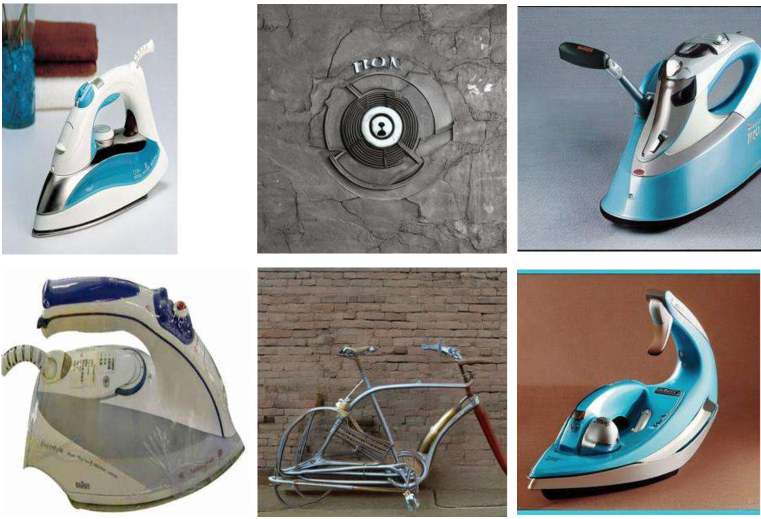
(a) iron

(b) carpenter’s plane

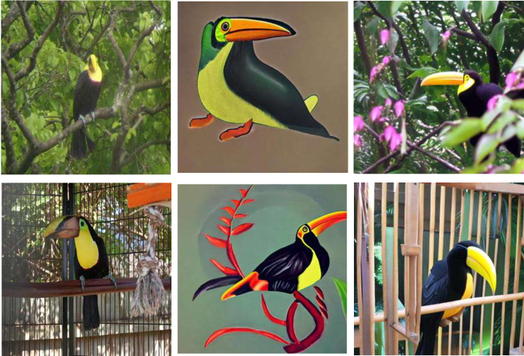
(c) tucan

Figure 3: Examples highlighting synthetic samples that are not close to the real data distribution and the need for dual text-image conditioning. Each subfigure depicts columns of images from left to right: ImageNet-LT, LDM (text), LDM(text and image). See also Figures 7, 8.

We identify three scenarios where using only text prompt results in synthetic samples that are not close to the real data used to train machine learning downstream models:

• Homonym ambiguity. A single text prompt can have multiple meanings. For example, consider generating data for the class iron that could either refer to the ironing machine or the metal element. See Figure 3 (a) for further illustrations.

• Text misinterpretation. The text-to-image generative model can produce images which are semantically inconsistent or partially consistent with the input prompt. An example of that is the class carpenter’s plane from ImageNet-LT. When prompted with this term, the diffusion model generated images of wooden planes instead of the intended carpentry tools. See Figure 3 (b) for further illustrations.

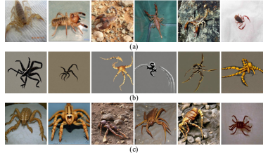
Figure 7: Here we plot more samples from Imagenet-LT where stylistic bias appears in synthetic generations. This scenario arises when the generative model produces images with a particular style for some prompts, which does not match the style of the real data. See Section 3.2 for more details. (a) real samples from class scorpian, (b) synthtic samples using LDM, (c) synthetic samples with image and text conditioning.

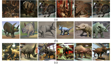
Figure 8: Here we plot more samples from Imagenet-LT where stylistic bias appears in synthetic generations. This scenario arises when the generative model produces images with a particular style for some prompts, which does not match the style of the real data. See Section 3.2 for more details. (a) real samples from class triceratops, (b) synthetic samples using LDM, (c) synthetic samples with image and text conditioning.

• Stylistic Bias. The generative model can produce images with a particular style for some prompts, which does not match the style of the real data. For instance, the Toucan images in the ImageNet-LT dataset are mostly real photographs, but the generative model frequently outputs drawings of this species of bird. See Figure 3 (c) for further illustrations. Also see more samples in Figures 7, 8.

To alleviate the above-described issues, we borrow from the generative models’ literature a dual-conditioning technique. In this approach, the generator is conditioned on both a text descriptor containing the class label and a randomly selected real image from the same class in the real training dataset. This additional layer of conditioning steers the diffusion model to generate samples which are more similar to those in the real training data; see Figure 3, to contrast samples from text-conditional models with those of text-and-image-conditional models. Using the unCLIP model in Rombach et al. (2022), the noise prediction network $\epsilon_{\theta}^{(t)}(\mathbf{x}_{t})$ in Equation 1 is extended to be a function of the conditioning image’s embedding, denoted as $\epsilon_{\theta}^{(t)}(\mathbf{x}_{t},\mathbf{z}_{\text{cond}})$, where $\mathbf{z}_{\text{cond}}$ is the CLIP embedding of the conditioning image.

3.3 Increasing the conditional diversity of synthetic data

As discussed in Section 3.2 leveraging conditioning from real images to synthesize data results in generating samples that are closer to the real data distribution. However, this comes at the cost of limiting the generative model’s ability to produce diverse images. Yet, such diversity is essential to train downstream classification models. We propose to apply random dropout on image embdding. Dropout is a technique used for preventing overfitting by randomly setting a fraction of input units to 0 at each update during training time (Srivastava et al., 2014). In this setup, the application of dropout serves a different yet equally crucial purpose: enhancing the diversity of generated images.

By applying random dropout to the embedding of the conditioning image, we effectively introduce variability into the information that guides the generative model. This stochasticity breaks the deterministic link between the conditioning image and the generated sample, thereby promoting diversity in the generated images. For instance, if the conditioning image contains a Persian Cat with a specific set of features (e.g., shape, color, background), dropout might nullify some of these features in the embedding, leading the generative model to explore other plausible variations of Persian Cat in Figure 4 (a, b). Intuitively, this diverse set of generated samples, which now contain both the core characteristics of the class and various incidental features, better prepares the downstream classification models for real-world scenarios where data can be highly heterogeneous..

Figure 4: Impact of dropout and Feedback-Guided (FG) sampling. Subfigures (a), (b) and (c) depicts regular sampling, sampling with dropout, and sampling with dropout and Feedback Guidance (Entropy), respectively. All samples are generated with the same seed. Also see Figures 9, 10.

4 Experiments

We explore two classification scenarios: (1) class-imbalanced classification, where we generate synthetic samples to create a balanced representation across classes; and (2) group-imbalanced classification, where we leverage synthetic data to achieve a balanced distribution across groups.

4.1 Class-imbalanced classification

Dataset. The ImageNet-LongTail (ImageNet-LT) dataset (Liu et al., 2019) is a subset of the original ImageNet (Deng et al., 2009) consisting of 115.8K images distributed non-uniformly across 1,000 classes. In this dataset, the number of images per class ranges from a minimum of 5 to a maximum of 1,280. However, the test and validation sets are balanced. In line with related literature (Shin et al., 2023), our goal is to synthesize missing data points in a way that, when combined with the real data, results in a uniform distribution of examples across all classes.

Experimental setup. We leverage the pre-trained state-of-the-art image-and-text conditional LDM v2-1-unclip (Rombach et al., 2022) to sample from. We adopt the widely used ResNext50 architecture as the classifier for all our experiments on ImageNet-LT. Our classifier is trained for 150 epochs. To improve model scaling with synthetic data, we modify the training process to include 50% real and 50% synthetic samples in each mini-batch.  We apply a balanced mini-batch approach when training all LDM methods. We also use the balanced Softmax (Ren et al., 2020) loss when training the classifier. For additional experimental details see Appendix G.

Metrics. We follow the standard protocol and report the overall average accuracy across classes, and the stratified accuracy across classes Many (any class with over 100 samples), Medium (any class with 100-20 samples), and Few (any class with less than 20 samples).

Baselines. We compare the proposed approach with prior art which does not leverage synthetic data from pre-trained generative models and with recent literature which does. We also compare the proposed approach with a vanilla sampling LDM that uses only the text prompts as conditioning. We report the results of our proposed framework for the three feedback guidance techniques introduced in section 3, namely, Loss, Hardness and Entropy. When leveraging synthetic data, we balance ImageNet-LT by generating as many samples as required to obtain 1,300 examples per class.

Method	# Syn. data	ImageNet-LT
		Overall	Many	Medium	Few
ERM (43)	✗	43.43	65.31	36.46	8.15
Decouple-cRT (32)	✗	47.3	58.8	44.0	26.1
Decouple-LWS (32)	✗	47.7	57.1	45.2	29.3
Remix (14)	✗	48.6	60.4	46.9	30.7
Balanced Softmax (49)	✗	51.0	60.9	48.8	32.1
Mix-Up GLMC  (18)	✗	57.21	64.76	55.67	42.19
Fill-Up (61)	2.6M	63.7	69.0	62.3	54.6
LDM (txt)	1.3M	57.90	64.77	54.62	50.30
LDM (txt and img)	1.3M	58.92	56.81	64.46	51.10
LDM-FG (Loss)	1.3M	60.41	66.14	57.68	54.1
LDM-FG (Hardness)	1.3M	56.70	58.07	55.38	57.32
LDM-FG (Entropy)	1.3M	64.7	69.8	62.3	59.1

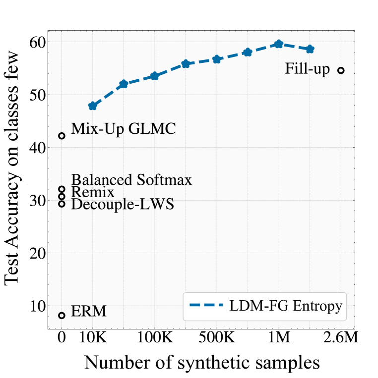
Figure 5: Classification accuracy on ImageNet-LT using ResNext50 backbone. In the table on the left we compare the performances of our model LDM-FG with respect to the current state-of-the art. In the figure on the right, we plot the performances on the class Few with respect to the number of synthetic data added during the classifier’s training.

Discussion. Figure  5 presents the results. We observe that approaches which do not leverage generated data exhibit the lowest accuracies across all groups, and overall, with Mix-Up obtaining the best results. It is worth noting that Mix-Up leverages advanced data augmentation strategies on the real data, which result in new samples. When comparing frameworks which use generated data from state of the art generative models, our framework surpasses the LDM baseline. Notably, the LDM with Feedback-Guidance (LDM-FG) based on the entropy criteria increases the LDM baseline performance $\sim 5$ points overall and, perhaps more interestingly, these improvements translate into a $\sim 9$ points boost on classes Few. Our best LDM-FG also surpasses the most recent competitor, Fill-Up  Shin et al. (2023), by $1\%$ accuracy point overall while using a half the amount of synthetic images. This highlights the importance of generating samples that are close to the real data distribution—as Fill-Up does— but also improving their diversity and usefulness.

4.2 Group-imbalanced classification

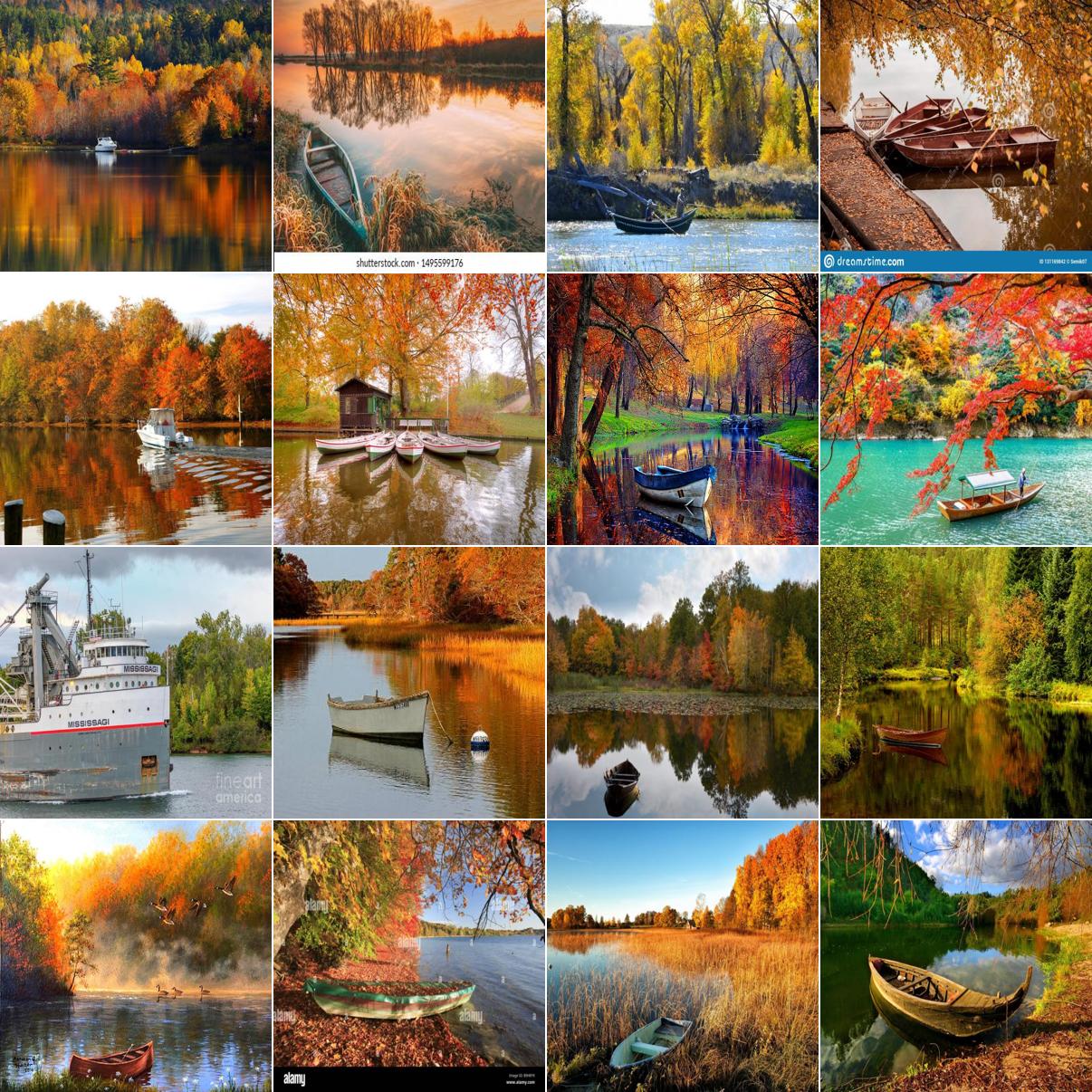
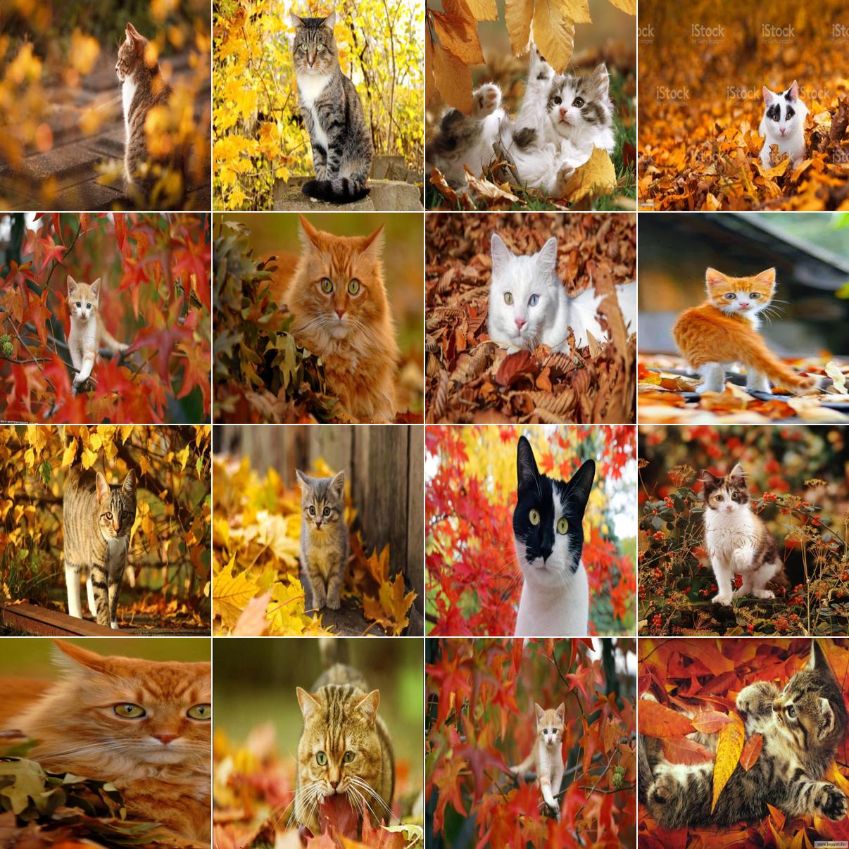
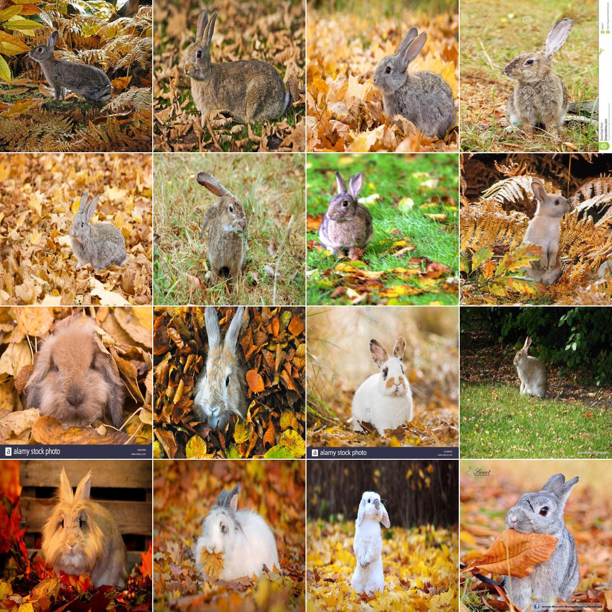
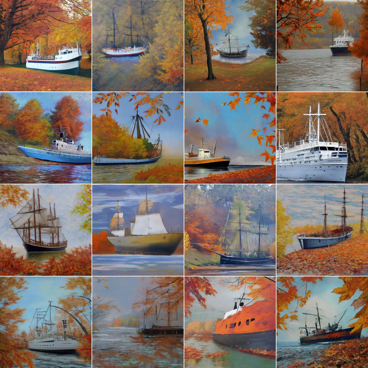
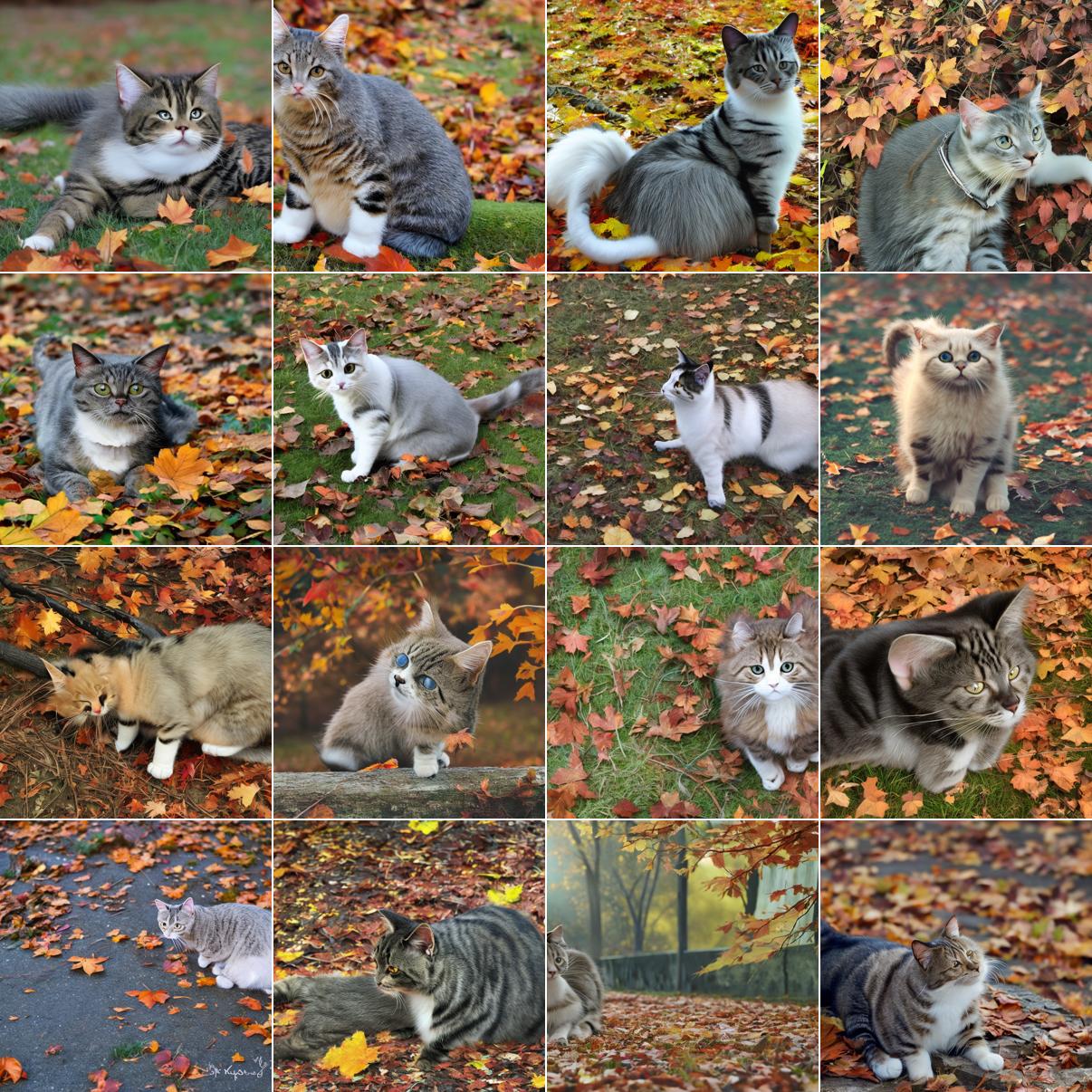
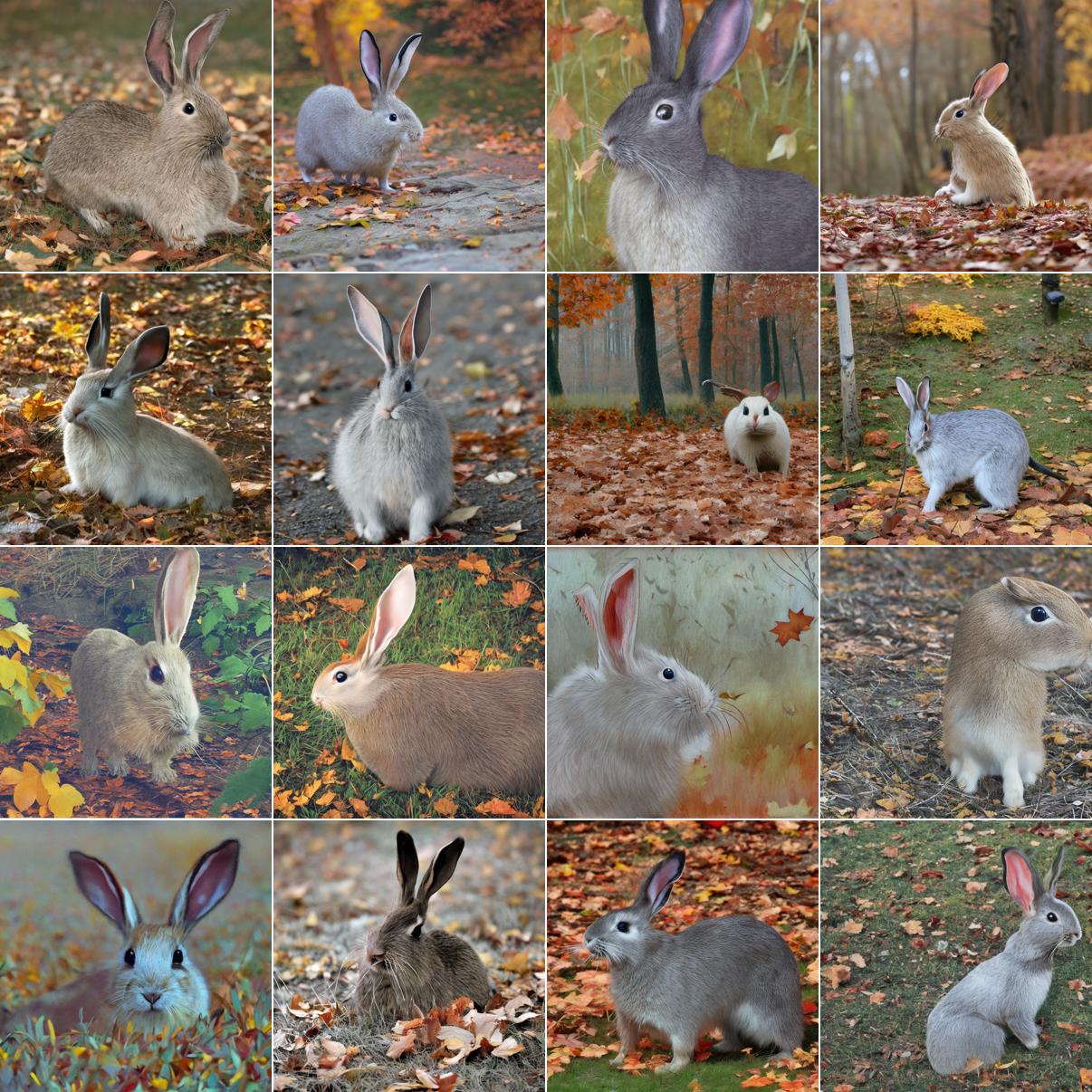
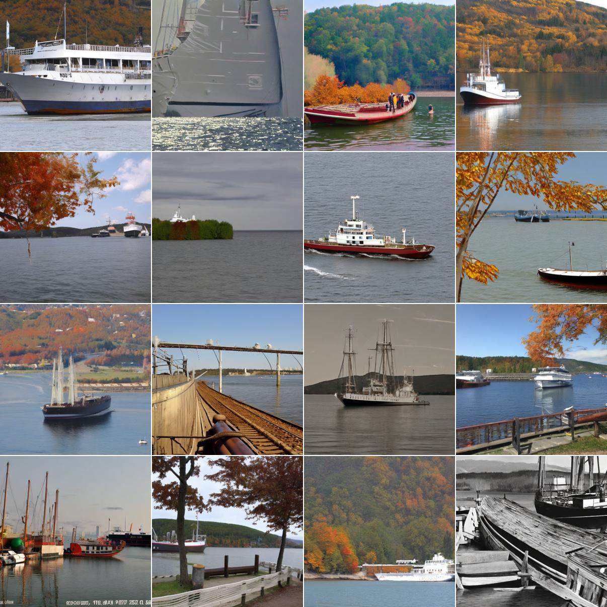
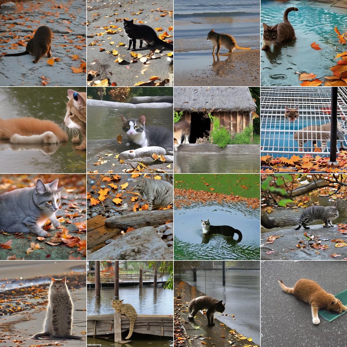
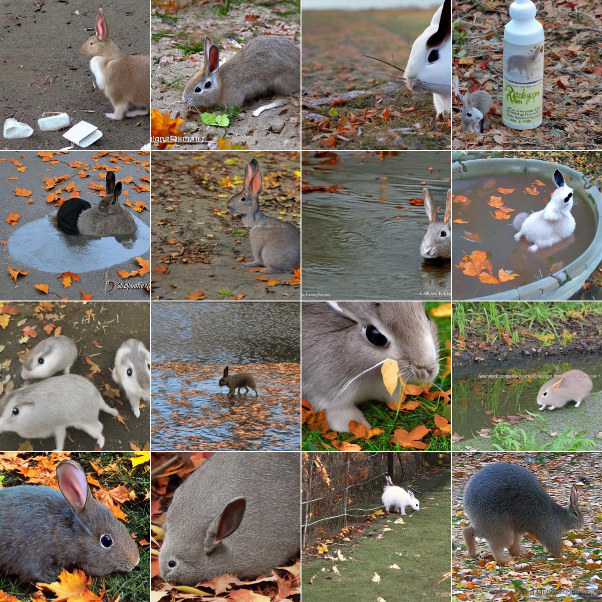
Figure 11: Synthetic samples of three different classes of NICO++. Column 1: class ship in context autumn, Column 2: class cat in context autumn , Column 3: class rabbit in autumn. First row: Real samples from NICO++, Second row: synthetic samples LDM. Third row: synthetic samples using Entropy as the guidance and dropout.

Dataset. We follow the sub-population shift setup of NICO++(Zhang et al., 2023) dataset introduced in Yang et al. (2023) which contains 62,657 training examples, 8,726 validation and 17,483 test examples. This dataset contains 60 classes of animals and objects within 6 different contexts (autumn, dim, grass, outdoor, rock, water). The pair of class-context is called a group, and the dataset is imbalanced accross groups. In the training set, the maximum number of examples in a group is 811 and the minimum is 0. For synthetic samples generated using our framework see Figure 11.

Experimental setup. We again leverage the pre-trained state-of-the-art image-and-text conditional LDM v2-1-unclip (Rombach et al., 2022) as high performant generative model to sample from. Since some groups in the dataset do not contain any real examples, we cannot condition the LDM model on random images from group, and so instead, we condition the LDM on random in-class examples. We adopt the ResNet50 (He et al., 2016) architecture as the classifier, given its ubiquitous use in prior literature. For each baseline, we train the classifier with five different random seeds.

Metrics. Following prior work on sub-population shift (Yang et al., 2023; Sagawa et al., 2019), we report worst-group accuracy (WGA) as the benchmark metric. We also report overall accuracy.

Baselines. We compare our framework against the NICO++ benchmark suite introduced in  Zhang et al. (2023); Yang et al. (2023). These state-of-the-art methods may leverage data augmentation but do not rely on synthetic data from generative models. We also consider a vanilla LDM baselines conditioned on text prompt, and report results for all three criteria. We generate the text prompts as class-label in context. We balance the NICO++ dataset such that each group has 811 samples, overall we generate 229k samples.

Table 1: Classification average and worst group accuracy on NICO++ dataset using ResNet50 pretrained on Imagenet.

Algorithm	# Syn. data	Avg. Accuracy	Worst Group Accuracy
ERM (Yang et al., 2023)	✗	85.3 $\pm$ 0.3	35.0 $\pm$ 4.1
Mixup (Zhang et al., 2017)	✗	84.0 $\pm$ 0.6	42.7 $\pm$ 1.4
GroupDRO (Sagawa et al., 2019)	✗	82.2 $\pm$ 0.4	37.8 $\pm$ 1.8
IRM (Arjovsky et al., 2019)	✗	84.4 $\pm$ 0.7	40.0 $\pm$ 0.0
LISA (Yao et al., 2022)	✗	84.7 $\pm$ 0.3	42.7 $\pm$ 2.2
BSoftmax (Ren et al., 2020)	✗	84.0 $\pm$ 0.5	40.4 $\pm$ 0.3
CRT (Kang et al., 2019)	✗	85.2 $\pm$ 0.3	43.3 $\pm$ 2.7
LDM	229k	86.02 $\pm$ 1.14	32.66 $\pm$ 1.33
LDM FG (Loss)	229k	84.55 $\pm$ 0.20	45.60$\pm$ 0.54
LDM FG (Hardness)	229k	84.66 $\pm$ 0.34	40.80 $\pm$ 0.97
LDM FG (Entropy)	229k	85.31 $\pm$ 0.30	49.20 $\pm$ 0.97

Discussion. Table 1 presents the average performance across five random seeds of our method in contrast with previous works. As shown in the table, our method achieves remarkable improvements over prior art which does not leverage synthetic data from generative models. More precisely, we observe notable WGA improvements of $\sim 6\%$ over the best previously reported results on the ResNet architecture. When comparing against baselines which do leverage synthetic data from state-of-the-art generative models, our framework remains competitive in terms of average accuracy, and importantly, surpasses the ERM baseline in terms of WGA by over $14\%$. The improvements over LDM further emphasize the benefit of generating samples that are close to the real data distribution, are diverse and useful when leveraging generated data for representation learning. Notably, the improvements achieved by our framework are observed for all the explored criteria, although entropy consistently yields the best results.

Also note that our framework tackles the group-imbalanced problem from the data perspective. Any algorithmic approach such as Bsoftmax (Ren et al., 2020), IRM (Arjovsky et al., 2019), or GroupDRO (Sagawa et al., 2019) can be applied on top of our approach.

4.3 Ablations

To validate the effect of dual image-text conditioning, dropout on the image conditioning embedding, and feedback-guidance, we perform an ablation study and report Fréchet Inception Distance (FID) (Heusel et al., 2017), density and coverage (Naeem et al., 2020), and average accuracy overall and on the classes Few. FID and density serve as a proxy to measure how close the generated samples are to the real data distribution. Coverage serves as proxy for diversity, and accuracy improvement for usefulness. FID, density and coverage are computed by generating 20 samples per class and using the ImageNet-LT validation set (20,000 samples) as reference. The accuracies are computed on the ImageNet-LT validation set. As shown in the Table 2, leveraging the vanilla sampling strategy of an LDM conditioned on text only (row 1) results in the worse performance across metrics. By leveraging image and text conditioning simultaneously (row 2) , we improve both FID and density, suggesting that generated samples are closer to the ImageNet-LT validation set. When applying dropout to the image embedding (row 3), we observe a positive effect on both FID and coverage, indicating a higher diversity of the generated samples. Finally, when adding feedback signals (rows 4–6), we notice the highest accuracy improvements (comparing to the model trained only on real data) both on average (except for hardness) and on the classes Few, highlighting the importance of leveraging feedback-guidance to improve the usefulness of the samples for representation learning downstream tasks. It is important to note that quality and diversity metrics such as FID, density and coverage may not be reflective of the usefulness of the generated synthetic samples (compare Hardness row with the Entropy row in Table 2).

Table 2: Ablation of our framework based on LDM. Results are computed w.r.t. the real balanced validation set of the ImageNetLT. All hyper-parameters for each setup are tuned.

Text	Img	dropout	FG	FID$\downarrow$	Density $\uparrow$	Coverage$\uparrow$	Avg. / Few validation acc. $\uparrow$
✓	✗	✗	✗	18.46	0.962	0.690	59.52 / 50.74
✓	✓	✗	✗	14.24	1.019	0.676	59.95 / 49.5
✓	✓	✓	✗	13.63	1.06	0.722	60.16 / 54.79
✓	✓	✓	Loss	18.48	0.8672	0.6398	62.19 / 54.78
✓	✓	✓	Hardness	10.84	1.07	0.82005	57.7 / 56.57
✓	✓	✓	Entopy	21.36	0.8217	0.6148	65.7 / 57.7

5 Related work

Synthetic Data for Training.

Synthetic data serves as a readily accessible source of data in the absence of real data. One line of previous works have used graphic-based synthetic datasets that are usually crafted through pre-defined pipelines using specific data sources such as 3D models or game engines Peng et al. (2017); Richter et al. (2016); Bordes et al. (2023); Richter et al. (2016); Peng et al. (2017) as synthetic data to train downstream models. Despite their utility, these methods suffer from multiple limitations, such as a quality gap with real-world data. Another set of prior work has considered using pre-trained GANs as data generators to yield augmentations to improve representation learning Astolfi et al. (2023); Chai et al. (2021); with only moderate success as the generated samples still exhibited limited diversity (Jahanian et al., 2021). More recent studies have begun to leverage pre-trained text-to-image diffusion models for improved classification (He et al., 2023; Sariyildiz et al., 2023; Shipard et al., 2023; Bansal & Grover, 2023; Dunlap et al., 2023) or other downstream tasks (Wu et al., 2023; You et al., 2023; Lin et al., 2023; Tian et al., 2023). For example, Imagen model (Saharia et al., 2022) was fine-tuned by Azizi et al. (2023) to improve Imagenet (Deng et al., 2009) per-class accuracy. Li et al. (2023) proposed ’diffusion classifier’, a pre-trained diffusion model adapted for the task of classification. He et al. (2023) adapted a diffusion model to generate images for fine-tuning CLIP Radford et al. (2021). Sariyildiz et al. (2023) showed that prompt-engineering can lead to a training data from which transferable representations can be learned. These studies suggest that it is possible to use features extracted from synthetic data for several downstream tasks. However, consistent with our findings, He et al. (2023) and Shin et al. (2023) argue that these methods may produce noisy, non-representative samples when applied to data-limited scenarios, such as those with long-tailed and open-ended distributions. Shin et al. (2023) uses textual inversion (Dhariwal & Nichol, 2021) in an image synthesis pipeline for long-tailed scenarios for improved domain alignment and classification accuracy. For related work on real data balancing methods for imbalanced datasets, see Appendix A.2.

6 Conclusion

We introduced a framework that leverages a pre-trained classifier together with a state-of-the-art text-and-image generative model to extend challenging long-tailed datasets with useful, diverse synthetic samples that are close to the real data distribution, with the goal of improving on downstream classification tasks. We achieved usefulness by incorporating feedback signals from the downstream classifier into the generative model; we employed dual image-text conditioning to generate samples that are close to the real data manifold and we improved the diversity of the generated samples by applying dropout to the image conditioning embedding. We substantiated the effect of each of the components in our framework through ablation studies. We validated the proposed framework on ImageNet-LT and NICO++, consistently surpassing prior art with notable improvements.

Limitations. Our approach inherits the limitations of the state-of-the-art generative models, namely the image realism and representation diversity are determined by the abilities of current generative model – our guidance mechanism can only explore the data manifold already captured by the generative model. In our work, we consider only one feedback cycle from a fully trained classifier. We leave for future exploration a setup where the feedback from the classifier is being sent to the generator online while the representation learning model is being trained.

Acknowledgement The authors would like to thank Mattie Tesfaldet, Pietro Astolfi, Oscar Mañas and other members of the FAIR team at Meta for useful discussions, feedback and support.

Appendix A Appendix

A.1 Derivation of equation 3

Simply writing the Bayes rule, we have:

$$\nabla_{x}\log p(x|h,y) =\nabla_{x}\log\left[\frac{p(x,h,y)}{p(h,y)}\right]=\nabla_{x}\log\left[\frac{p(h|x,y)p(x|y)p(y)}{p(h|y)p(y)}\right]$$

$$=\nabla_{x}\log\left[p(h|x,y)p(x|y)\right]=\nabla_{x}\log p(x|y)+\nabla_{x}\log p(h|x,y).$$ (9)

Note that by using a pre-trained diffusion model, we have access to the estimated class conditional score function $\nabla_{x}\log\ \hat{p}_{\theta}(x|y)$. We then assume there exists a criterion function $\mathcal{C}(x,y,f_{\phi})$ that evaluates the usefulness of a sample $x$ based on the classifier $f_{\phi}$. Consequently, we model $p(h|x,y)$ as:

$$p(h|x,y)=\frac{\exp\left(\mathcal{C}(x,y,f_{\phi})\right)}{\mathcal{Z}},$$ (10)

where $\mathcal{Z}$ is a normalizing constant. As a result, we can generate useful samples based on the criteria function $\mathcal{C}(x,y,f_{\phi})$, and following Eq. A.1, we have:

$$\nabla_{x}\log\hat{p}_{\omega}(x|h,y)=\nabla_{x}\log\ \hat{p}_{\theta}(x|y)+\omega\nabla_{x}\mathcal{C}(x,y,f_{\phi}),$$ (11)

where $\omega$ is a scaling factor that controls the strength of the signal from our criterion function $\mathcal{C}$. Following Eq. 2, we have,

$$\nabla_{x}\log\hat{p}_{\omega}(x|h,y)=\nabla_{x}\log\hat{p}_{\theta}(x)+\gamma\nabla_{x}\log\hat{p}_{\theta}(y|x)+\omega\nabla_{x}\mathcal{C}(x,y,f_{\phi}).$$ (12)

A.2 Related Work: Balancing Methods for Imbalanced Datasets.

An effective strategy for mitigating class imbalance include balancing the dataset (Shelke et al., 2017; Idrissi et al., 2022; Shen et al., 2016; Park et al., 2022; Liu et al., 2019). Dataset balancing can either involve up-sampling the minority classes to bring about a uniform class/group distribution or sub-sampling the majority classes to match the size of the smallest class/group. Traditional up-sampling methods usually involve either replicating minority samples or through simple methods such as linearly interpolating between them. However, such simple up-sampling techniques have been found to be less effective in scenarios with limited data (Hu et al., 2015). Sub-sampling is generally more effective, but it carries the risk of overfitting due to reduced dataset size. Another line of research focuses on re-weighting techniques (Sagawa et al., 2019; Samuel & Chechik, 2021; Cao et al., 2019; Ren et al., 2020; Cui et al., 2019). These methods scale the importance of underrepresented classes or groups according to specific criterion, such as their count in the dataset or the loss incurred during training (Liu et al., 2021). Some approaches adapt the loss function itself or introduce a regularization technique to achieve a more balanced classification performance (Ryou et al., 2019; Lin et al., 2017; Pezeshki et al., 2021). Another effective method is the Balanced Softmax (Ren et al., 2020) that adjusts the biases in the softmax layer of the classifier to counteract imbalances in class distribution.

A.3 A Toy 2-dimensional Example of Criteria Guidance

Figure 6 illustrates the experimental results of using a simple 2-dimensional dataset for a classification task. The dataset contains two classes represented by blue and red data points. Within each class, the data consists of two modes: the majority mode, containing 90% of the data points, and the minority mode, which holds the remaining 10%. We initially train a diffusion model on this dataset. Sampling from the trained diffusion model generates synthetic data that closely follows the distribution of the original training data, showing an imbalance between the modes of each class (see Figure 6 (b)).

To encourage generation of data from the mode with lower density, we introduce a binary variable $h$ into the model. In this context, $h=0$ indicates the minority mode, while $h=1$ signifies the majority mode. Following the criteria guidance discussed in Section 3.1.1, without retraining the model, we modify the sampling process so that the generator is guided towards generating samples of higher entropy. To that end, we train a linear classifier for several epochs until it effectively classifies the majority mode, but the decision boundary intersects the minority mode, resulting in misclassification of those points. Leveraging the classifier’s uncertainty around this decision boundary, we guide the generative model to produce higher entropy samples. This results in more synthetic samples being generated from the minority modes of each class (see Figure 6 (c)).

Integrating this synthetic data with the original data produces a more uniform distribution across modes, leading to a more balanced classifier. This is desirable in our context as it mitigates the biases inherent in the original dataset and improves the model’s generalization.

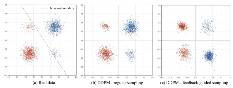
Figure 6: Experimental results on a 2-dimensional classification dataset showcasing the effect of feedback-guided sampling. Panel (a): Real data consists of two classes represented by blue and red data points. Within each class, two modes are identified: a majority mode comprising 90% of the data and a minority mode containing the remaining 10%. Panel (b): The synthetic data generated by regular sampling of a DDPM replicates the imbalances of the original dataset. Panel (c): Synthetic data generated after modifying the diffusion model guided by feedback from a linear classifier. Feedback-guided sampling leads to more samples being generated from the minority modes. Combining with real data, it results in more balanced data with increased representation from the minority mode, ultimately improving classifier performance.

Appendix B Samples Stylistic Bias

Stylistic Bias is one of the challenges in synthetic data generation where the generative model consistently produces images with a particular style for some prompts, which does not correspond to the style of the real data. This results in a mismatch between synthetic and real data, potentially impacting the performance of machine learning models trained on such data.

Appendix C Samples for Dropout on Image Embedding

Dropout introduces variability into the information that guides the generative model by randomly omitting certain features from the conditioning image embedding. This stochasticity breaks the deterministic relationship between the conditioning image and the generated sample, leading to increased diversity in the generated images. See Figure 9.

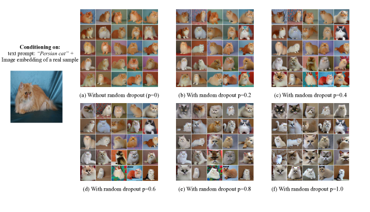
Figure 9: Synthetic sample generation using text prompt and image embedding. We plot different levels of dropout. We condition on a single random real sample (plotted on the left most). As observed, using only image conditioning and text (a), we observe very low diversity in the generations. As we increase the dropout probability, we observe more diversity. If we only condition on the text prompt (f), we also observe low diversity.

Appendix D Samples Feedback Guided Sampling

In this section we provide more synthetic samples using Feedback guided sampling. See Figure 10 and 11 for more details.

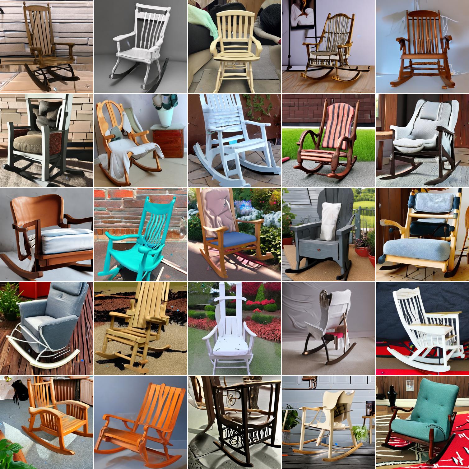
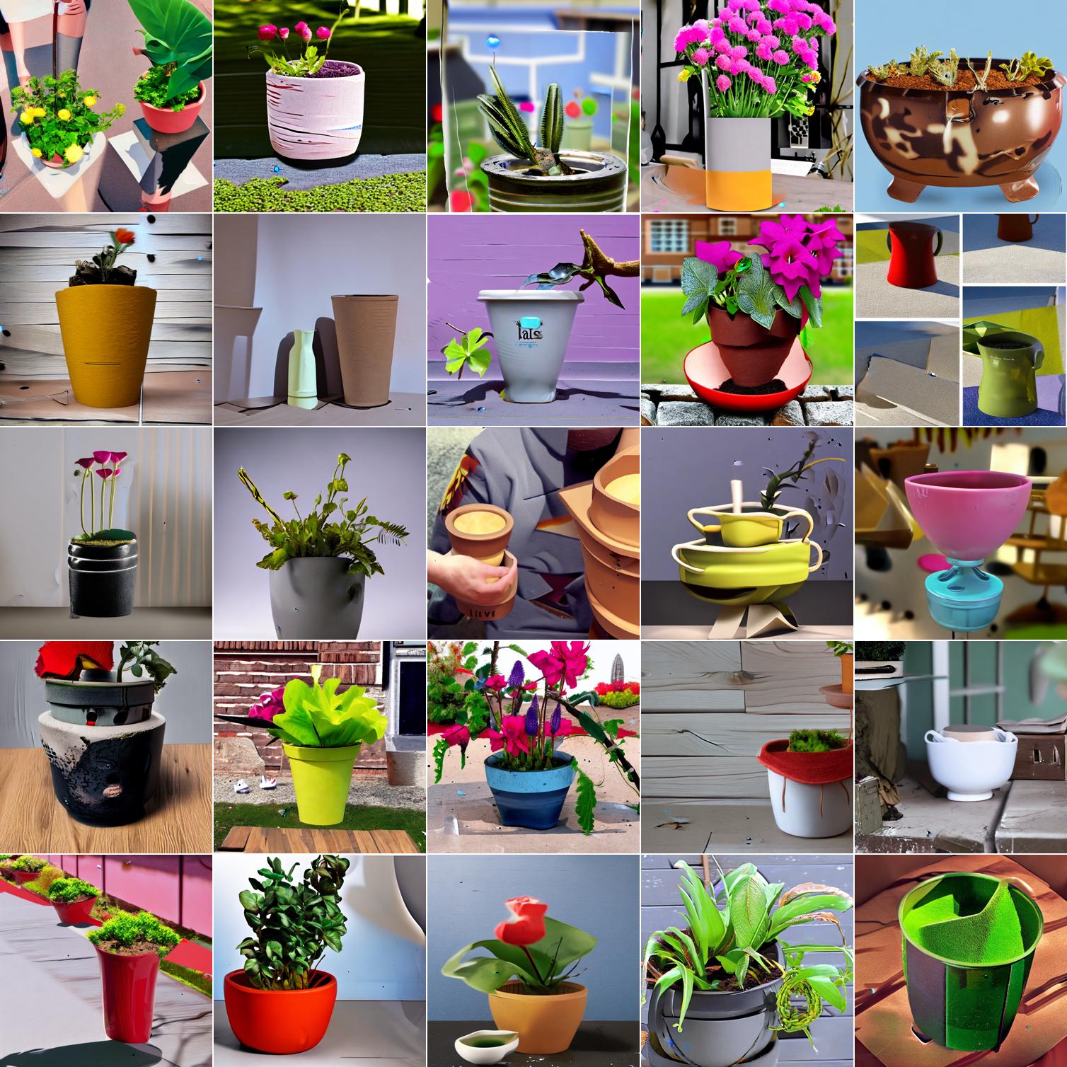
Figure 10: Synthetic samples of three different classes of Imagenet-LT. Column 1: class rocking chair, Column 2: class flower pot. First row: Real samples from Imagenet-LT, Second row: synthetic samples vanilla LDM. Third row: synthetic samples using Entropy as the guidance.

D.1 The interplay between clip-guidance and feedback-guidance

Figures 12, 13, and 14 display grids of synthetically generated images. Each is conditioned to generate the class ”African Chameleon”, with variations in feedback-guidance scales based on three different criteria: entropy, loss, and hardness. The grids are organized such that rows and columns correspond to varying levels of two distinct guidance scales: clip-guidance and feedback-guidance. Clip-guidance serves the role of ensuring that the generated images are faithful to the visual characteristics of an ”African Chameleon”, such as color patterns, skin details, or posture. On the other hand, feedback-guidance relies on the uncertainties in the classifier’s predictions to guide the generative model.

As we move from left to right along the columns, the clip-guidance scale increases, thereby leading to images that become increasingly accurate and recognizable as chameleons. These images would likely be easier for both humans and classifiers to correctly identify as representing the African Chameleon class.

Conversely, when we move from the top row to the bottom, the feedback-guidance scale increases. This change leads to the generative model generating more challenging images. These images diverge from the standard or typical depictions of a chameleon, thus posing a greater challenge for the classifier.

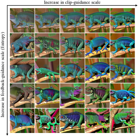
Figure 12: A grid of images generated for the class ”African Chameleon”. Along the x-axis, from left to right, the clip-guidance scale is increased, while along the y-axis, from top to bottom, the classifier-feedback guidance scale is increased. The random seed is consistent across all images, ensuring that any observed variations are only due to changes in the guidance scales. Moving from left to right, it is evident that increasing the clip guidance scale results in samples that more faithful to the ”African Chameleon” class. However, this comes at the cost of generating very typical, easily classifiable images. Conversely, as we move from top to bottom, increasing the classifier-feedback guidance results in the generation of more ’challenging’ or atypical images of African chameleon.

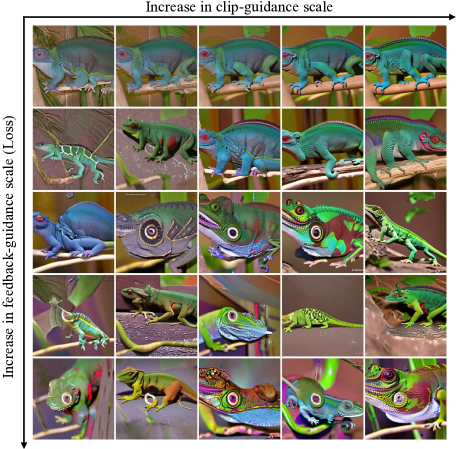
Figure 13: A grid of images generated based on the ’loss’ criterion for the class ”African Chameleon”. Like Figure 12, as the clip guidance scale increases from left to right, images become more faithful to the class, while increasing the classifier-feedback guidance from top to bottom produces more atypical images.

Figure 14: A grid of images generated based on the ’hardness’ criterion for the class ”African Chameleon”. As with Figures 12 and 13, variations in the images are due to changes in the clip and classifier-feedback guidance scales.

Appendix E Impact of the number of generated images

Figure 15 shows the performances on a classifier trained on ImageNet-LT when using a different amount of generated images. We show that adding generated synthetic data significantly help to increase the overall performance of the model. In addition, we observe significant gain on the few classes which highlight that generated images are well-suited for imbalanced real data scenarios.

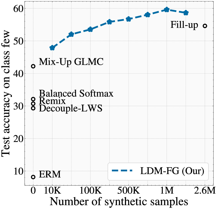
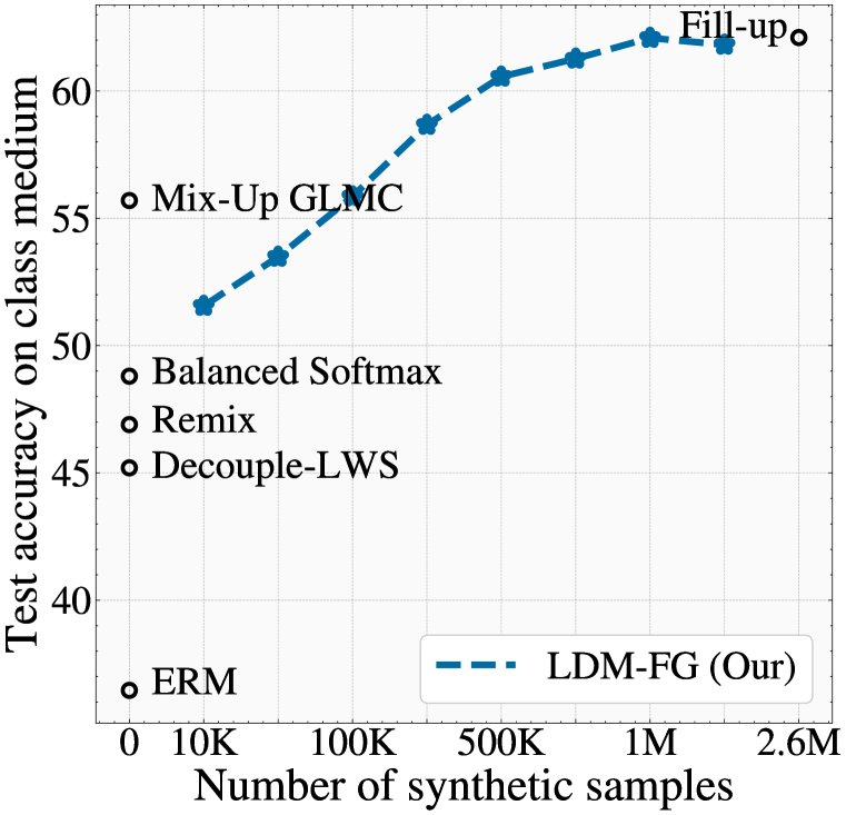
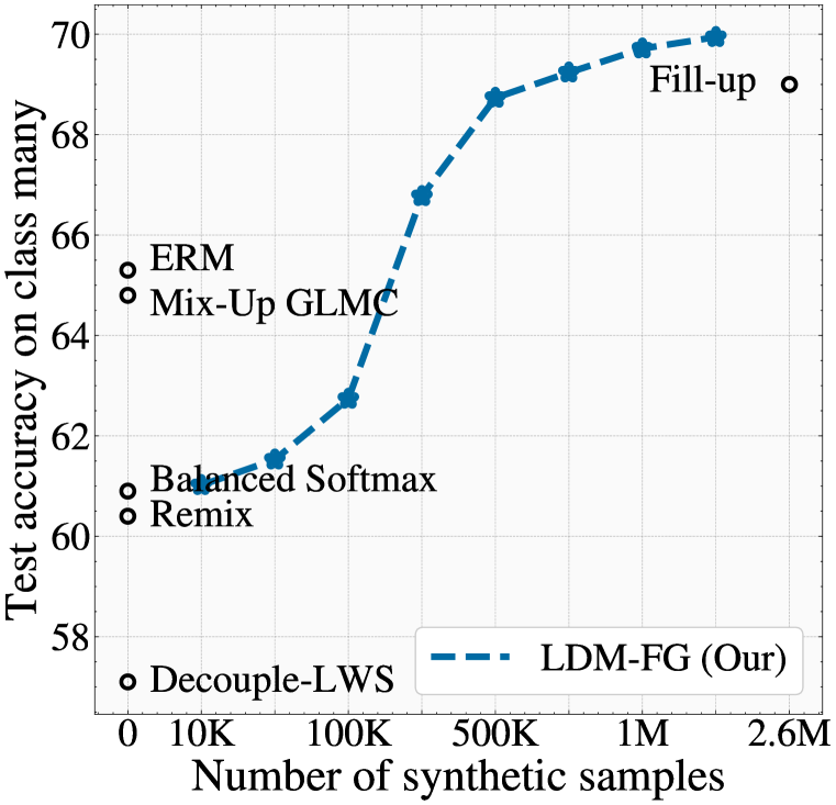
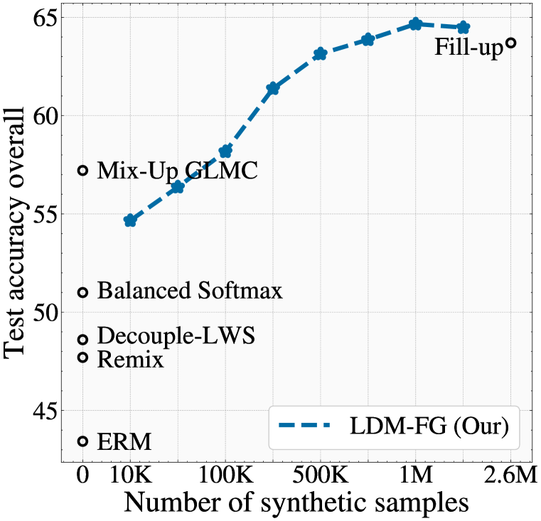
Figure 15: Test accuracy depending on the number of generated synthetic data used to train the classifier. The first curve shows the accuracy on the class Few, while the second one shows the accuracy on the class Medium and the last one shows the accuracy on class Many. Our method significantly outperforms Fill-Up(Shin et al., 2023) while using less synthetic data.

Appendix F Impact of using balanced softmax with synthetic data

In our experiments, we have used balanced softmax to train our classifier to increase the performances on class Few. We also ran experiments using a weighted average of a traditional cross-entropy loss using balanced softmax with the same loss without balanced softmax. In this experiment, we added a scalar coefficient $\alpha$ which controls the weight of the balanced softmax loss in contrast to the standard loss. In Figure 16, we plot the test accuracy with respect to this balanced softmax weight. Without balanced softmax, the accuracy on the class many is extremely high while the accuracy on class few is much lower. However by increasing the balanced softmax coefficient, we significantly increase the performances on class few and medium as well as the overall accuracy. However, this comes at the price of lower performance for classes Many.

Figure 16: Test accuracy on Few, Medium, Many and Overall with respect to the balanced softmax coefficient. All the models use 1.3M synthetic samples.

Appendix G Experimental Details

General setup in sample generation

We use the LDM v2-1-unclip (Rombach et al., 2022) as the state-of-the-art latent diffusion model that supports dual image-text conditioning. We use a pretrained classifier on the real data to guide the sampling process of the LDM. For Imagenet-LT, the classifier is trained using ERM with learning rate of $0.1$ (decaying) and weight-decay of $0.0005$ and batch-size of $32$. For NICO++ we use a pre-trained classifier on Imagnet and then fine-tune it on NICO++.

We apply 30 steps of reverse diffusion during the sampling. To apply different criteria in the sampling process, we use the pretrained classifier on the real data. For lower computational complexity, we use float16 datatype in PyTorch. Furthermore, we apply the gradient of the criterion function every 5 steps. So for 30 reverse steps, we only compute and apply the criterion 6 times. Through experiments we find that 5 is optimal as the generated samples look very similar to applying the criterion in every step.

For the hardness criterion in Eq. 3.1.1 where we need the $\mu_{y}$ and $\Sigma_{y}^{-1}$ for each class, we pre-compute these values. We compute the mean and covariance inverse of the feature representation of the classifier over all real samples. These values are then loaded and used during the sampling process.

G.1 ImageNet-LT

We follow the setup in Kang et al. (2019) and use a ResNext50 architecture. We apply the balanced softmax for all the LDM models reported for Imagenet-LT. We train the classifier for 150 epochs with a batch size of 512. We also use standard data augmentations such a random cropping, color-jittering, blur and grayscale during training.

G.2 NICO++

We follow the setup in Yang et al. (2023), where a pre-trained ResNet50 model on ImageNet is used for all the methods. We assume access to the attributes labels (contexts). For training our LDM model we only apply ERM without any extra algorithmic changes. We use the SGD with momentum of 0.9 and train for 50 epochs. We apply standard data augmentation such as resize and center crop and apply ImageNet statistics normalization.

Following the setup in Yang et al. (2023), for every method, we try 10 sets of hyper-parameters (learning rate, batch-size). We perform model selection and early stopping based on average validation accuracy. We then train the selected model on 5 random seeds and report the test performance.

References

- Arjovsky et al. (2019) Martin Arjovsky, Léon Bottou, Ishaan Gulrajani, and David Lopez-Paz. Invariant risk minimization. arXiv preprint arXiv:1907.02893, 2019.
- Astolfi et al. (2023) Pietro Astolfi, Arantxa Casanova, Jakob Verbeek, Pascal Vincent, Adriana Romero-Soriano, and Michal Drozdzal. Instance-conditioned gan data augmentation for representation learning, 2023.
- Azizi et al. (2023) Shekoofeh Azizi, Simon Kornblith, Chitwan Saharia, Mohammad Norouzi, and David J Fleet. Synthetic data from diffusion models improves imagenet classification. arXiv preprint arXiv:2304.08466, 2023.
- Balaji et al. (2022) Yogesh Balaji, Seungjun Nah, Xun Huang, Arash Vahdat, Jiaming Song, Karsten Kreis, Miika Aittala, Timo Aila, Samuli Laine, Bryan Catanzaro, et al. ediffi: Text-to-image diffusion models with an ensemble of expert denoisers. arXiv preprint arXiv:2211.01324, 2022.
- Bansal & Grover (2023) Hritik Bansal and Aditya Grover. Leaving Reality to Imagination: Robust Classification via Generated Datasets. In International Conference on Learning Representations (ICLR) Workshop, 2023.
- Bianchi et al. (2022) Federico Bianchi, Pratyusha Kalluri, Esin Durmus, Faisal Ladhak, Myra Cheng, Debora Nozza, Tatsunori Hashimoto, Dan Jurafsky, James Zou, and Aylin Caliskan. Easily accessible text-to-image generation amplifies demographic stereotypes at large scale, 2022.
- Blattmann et al. (2022) Andreas Blattmann, Robin Rombach, Kaan Oktay, Jonas Müller, and Björn Ommer. Semi-parametric neural image synthesis. Advances in Neural Information Processing Systems, 11, 2022.
- Bordes et al. (2022) Florian Bordes, Randall Balestriero, and Pascal Vincent. High fidelity visualization of what your self-supervised representation knows about. Transactions on Machine Learning Research, 2022. URL https://openreview.net/forum?id=urfWb7VjmL.
- Bordes et al. (2023) Florian Bordes, Shashank Shekhar, Mark Ibrahim, Diane Bouchacourt, Pascal Vincent, and Ari S Morcos. Pug: Photorealistic and semantically controllable synthetic data for representation learning. arXiv preprint arXiv:2308.03977, 2023.
- Cao et al. (2019) Kaidi Cao, Colin Wei, Adrien Gaidon, Nikos Arechiga, and Tengyu Ma. Learning imbalanced datasets with label-distribution-aware margin loss. Conference on Neural Information Processing Systems (NeurIPS), 2019.
- Casanova et al. (2021) Arantxa Casanova, Marlene Careil, Jakob Verbeek, Michal Drozdzal, and Adriana Romero Soriano. Instance-conditioned gan. Advances in Neural Information Processing Systems, 34:27517–27529, 2021.
- Chai et al. (2021) Lucy Chai, Jun-Yan Zhu, Eli Shechtman, Phillip Isola, and Richard Zhang. Ensembling with deep generative views. In IEEE Conference on Computer Vision and Pattern Recognition (CVPR), 2021.
- Cho et al. (2022) Jaemin Cho, Abhay Zala, and Mohit Bansal. Dall-eval: Probing the reasoning skills and social biases of text-to-image generative transformers. 2022.
- Chou et al. (2020) Hsin-Ping Chou, Shih-Chieh Chang, Jia-Yu Pan, Wei Wei, and Da-Cheng Juan. Remix: rebalanced mixup. In European Conference on Computer Vision (ECCV) Workshop, 2020.
- Cui et al. (2019) Yin Cui, Menglin Jia, Tsung-Yi Lin, Yang Song, and Serge Belongie. Class-balanced loss based on effective number of samples. In IEEE Conference on Computer Vision and Pattern Recognition (CVPR), 2019.
- Deng et al. (2009) Jia Deng, Wei Dong, Richard Socher, Li-Jia Li, Kai Li, and Fei-Fei Li. ImageNet: A large-scale hierarchical image database. In IEEE Conference on Computer Vision and Pattern Recognition (CVPR), 2009.
- Dhariwal & Nichol (2021) Prafulla Dhariwal and Alex Nichol. Diffusion models beat gans on image synthesis. In Conference on Neural Information Processing Systems (NeurIPS), 2021.
- Du et al. (2023) Fei Du, Peng Yang, Qi Jia, Fengtao Nan, Xiaoting Chen, and Yun Yang. Global and local mixture consistency cumulative learning for long-tailed visual recognitions. In Proceedings of the IEEE/CVF Conference on Computer Vision and Pattern Recognition, pp. 15814–15823, 2023.
- Dunlap et al. (2023) Lisa Dunlap, Alyssa Umino, Han Zhang, Jiezhi Yang, Joseph E Gonzalez, and Trevor Darrell. Diversify your vision datasets with automatic diffusion-based augmentation. arXiv preprint arXiv:2305.16289, 2023.
- Gu et al. (2023) Jindong Gu, Zhen Han, Shuo Chen, Ahmad Beirami, Bailan He, Gengyuan Zhang, Ruotong Liao, Yao Qin, Volker Tresp, and Philip Torr. A systematic survey of prompt engineering on vision-language foundation models. arXiv preprint arXiv:2307.12980, 2023.
- Hall et al. (2023) Melissa Hall, Candace Ross, Adina Williams, Nicolas Carion, Michal Drozdzal, and Adriana Romero Soriano. Dig in: Evaluating disparities in image generations with indicators for geographic diversity, 2023.
- He et al. (2016) Kaiming He, Xiangyu Zhang, Shaoqing Ren, and Jian Sun. Deep residual learning for image recognition. In Proceedings of the IEEE conference on computer vision and pattern recognition, pp. 770–778, 2016.
- He et al. (2023) Ruifei He, Shuyang Sun, Xin Yu, Chuhui Xue, Wenqing Zhang, Philip Torr, Song Bai, and XIAOJUAN QI. IS SYNTHETIC DATA FROM GENERATIVE MODELS READY FOR IMAGE RECOGNITION? In International Conference on Learning Representations (ICLR), 2023.
- Heusel et al. (2017) Martin Heusel, Hubert Ramsauer, Thomas Unterthiner, Bernhard Nessler, Günter Klambauer, and Sepp Hochreiter. Gans trained by a two time-scale update rule converge to a nash equilibrium. CoRR, abs/1706.08500, 2017. URL http://arxiv.org/abs/1706.08500.
- Ho & Salimans (2022) Jonathan Ho and Tim Salimans. Classifier-free diffusion guidance. arXiv preprint arXiv:2207.12598, 2022.
- Ho et al. (2020) Jonathan Ho, Ajay Jain, and Pieter Abbeel. Denoising diffusion probabilistic models. In Conference on Neural Information Processing Systems (NeurIPS), 2020.
- Hu et al. (2015) Yong Hu, Dongfa Guo, Zengwei Fan, Chen Dong, Qiuhong Huang, Shengkai Xie, Guifang Liu, Jing Tan, Boping Li, Qiwei Xie, et al. An improved algorithm for imbalanced data and small sample size classification. Journal of Data Analysis and Information Processing, 3(03):27, 2015.
- Hu et al. (2023) Yushi Hu, Benlin Liu, Jungo Kasai, Yizhong Wang, Mari Ostendorf, Ranjay Krishna, and Noah A Smith. Tifa: Accurate and interpretable text-to-image faithfulness evaluation with question answering. arXiv preprint arXiv:2303.11897, 2023.
- Idrissi et al. (2022) Badr Youbi Idrissi, Martin Arjovsky, Mohammad Pezeshki, and David Lopez-Paz. Simple data balancing achieves competitive worst-group-accuracy. In Conference on Causal Learning and Reasoning, pp. 336–351. PMLR, 2022.
- Jahanian et al. (2021) Ali Jahanian, Xavier Puig, Yonglong Tian, and Phillip Isola. Generative models as a data source for multiview representation learning. arXiv preprint arXiv:2106.05258, 2021.
- Kang et al. (2019) Bingyi Kang, Saining Xie, Marcus Rohrbach, Zhicheng Yan, Albert Gordo, Jiashi Feng, and Yannis Kalantidis. Decoupling representation and classifier for long-tailed recognition. arXiv preprint arXiv:1910.09217, 2019.
- Kang et al. (2020) Bingyi Kang, Saining Xie, Marcus Rohrbach, Zhicheng Yan, Albert Gordo, Jiashi Feng, and Yannis Kalantidis. Decoupling Representation and Classifier for Long-Tailed Recognition. In International Conference on Learning Representations (ICLR), 2020.
- Kang et al. (2023) Minguk Kang, Jun-Yan Zhu, Richard Zhang, Jaesik Park, Eli Shechtman, Sylvain Paris, and Taesung Park. Scaling up GANs for Text-to-Image Synthesis. In Proceedings of the IEEE Conference on Computer Vision and Pattern Recognition (CVPR), 2023.
- Lester et al. (2021) Brian Lester, Rami Al-Rfou, and Noah Constant. The power of scale for parameter-efficient prompt tuning. arXiv preprint arXiv:2104.08691, 2021.
- Li et al. (2023) Alexander C Li, Mihir Prabhudesai, Shivam Duggal, Ellis Brown, and Deepak Pathak. Your Diffusion Model is Secretly a Zero-Shot Classifier. arXiv preprint arXiv:2303.16203, 2023.
- Lin et al. (2023) Shaobo Lin, Kun Wang, Xingyu Zeng, and Rui Zhao. Explore the Power of Synthetic Data on Few-shot Object Detection. arXiv preprint arXiv:2303.13221, 2023.
- Lin et al. (2017) Tsung-Yi Lin, Priya Goyal, Ross Girshick, Kaiming He, and Piotr Dollár. Focal loss for dense object detection. In IEEE International Conference on Computer Vision (ICCV), 2017.
- Liu et al. (2021) Evan Z Liu, Behzad Haghgoo, Annie S Chen, Aditi Raghunathan, Pang Wei Koh, Shiori Sagawa, Percy Liang, and Chelsea Finn. Just train twice: Improving group robustness without training group information. In International Conference on Machine Learning, pp. 6781–6792. PMLR, 2021.
- Liu et al. (2019) Ziwei Liu, Zhongqi Miao, Xiaohang Zhan, Jiayun Wang, Boqing Gong, and Stella X Yu. Large-scale long-tailed recognition in an open world. In IEEE Conference on Computer Vision and Pattern Recognition (CVPR), 2019.
- Luccioni et al. (2023) Alexandra Sasha Luccioni, Christopher Akiki, Margaret Mitchell, and Yacine Jernite. Stable bias: Analyzing societal representations in diffusion models, 2023.
- Naeem et al. (2020) Muhammad Ferjad Naeem, Seong Joon Oh, Youngjung Uh, Yunjey Choi, and Jaejun Yoo. Reliable fidelity and diversity metrics for generative models. 2020.
- Nichol et al. (2022) Alexander Quinn Nichol, Prafulla Dhariwal, Aditya Ramesh, Pranav Shyam, Pamela Mishkin, Bob Mcgrew, Ilya Sutskever, and Mark Chen. GLIDE: Towards Photorealistic Image Generation and Editing with Text-Guided Diffusion Models. In International Conference on Machine Learning (ICML), 2022.
- Park et al. (2022) Seulki Park, Youngkyu Hong, Byeongho Heo, Sangdoo Yun, and Jin Young Choi. The majority can help the minority: Context-rich minority oversampling for long-tailed classification. In IEEE Conference on Computer Vision and Pattern Recognition (CVPR), 2022.
- Peng et al. (2017) Xingchao Peng, Ben Usman, Neela Kaushik, Judy Hoffman, Dequan Wang, and Kate Saenko. Visda: The visual domain adaptation challenge. arXiv preprint arXiv:1710.06924, 2017.
- Pezeshki et al. (2021) Mohammad Pezeshki, Oumar Kaba, Yoshua Bengio, Aaron C Courville, Doina Precup, and Guillaume Lajoie. Gradient starvation: A learning proclivity in neural networks. Advances in Neural Information Processing Systems, 34:1256–1272, 2021.
- Radford et al. (2021) Alec Radford, Jong Wook Kim, Chris Hallacy, Aditya Ramesh, Gabriel Goh, Sandhini Agarwal, Girish Sastry, Amanda Askell, Pamela Mishkin, Jack Clark, et al. Learning transferable visual models from natural language supervision. In International Conference on Machine Learning (ICML), 2021.
- Ramesh et al. (2021) Aditya Ramesh, Mikhail Pavlov, Gabriel Goh, Scott Gray, Chelsea Voss, Alec Radford, Mark Chen, and Ilya Sutskever. Zero-shot text-to-image generation. In International Conference on Machine Learning (ICML), 2021.
- Ramesh et al. (2022) Aditya Ramesh, Prafulla Dhariwal, Alex Nichol, Casey Chu, and Mark Chen. Hierarchical Text-Conditional Image Generation with CLIP Latents. arXiv preprint arXiv:2204.06125, 2022.
- Ren et al. (2020) Jiawei Ren, Cunjun Yu, Xiao Ma, Haiyu Zhao, Shuai Yi, et al. Balanced meta-softmax for long-tailed visual recognition. Advances in neural information processing systems, 33:4175–4186, 2020.
- Richter et al. (2016) Stephan R Richter, Vibhav Vineet, Stefan Roth, and Vladlen Koltun. Playing for data: Ground truth from computer games. In European Conference on Computer Vision (ECCV), 2016.
- Rombach et al. (2022) Robin Rombach, Andreas Blattmann, Dominik Lorenz, Patrick Esser, and Björn Ommer. High-resolution image synthesis with latent diffusion models. In IEEE Conference on Computer Vision and Pattern Recognition (CVPR), 2022.
- Ryou et al. (2019) Serim Ryou, Seong-Gyun Jeong, and Pietro Perona. Anchor loss: Modulating loss scale based on prediction difficulty. In IEEE International Conference on Computer Vision (ICCV), 2019.
- Sagawa et al. (2019) Shiori Sagawa, Pang Wei Koh, Tatsunori B Hashimoto, and Percy Liang. Distributionally robust neural networks for group shifts: On the importance of regularization for worst-case generalization. arXiv preprint arXiv:1911.08731, 2019.
- Saharia et al. (2022) Chitwan Saharia, William Chan, Saurabh Saxena, Lala Li, Jay Whang, Emily Denton, Seyed Kamyar Seyed Ghasemipour, Burcu Karagol Ayan, S Sara Mahdavi, Rapha Gontijo Lopes, et al. Photorealistic Text-to-Image Diffusion Models with Deep Language Understanding. arXiv preprint arXiv:2205.11487, 2022.
- Samuel & Chechik (2021) Dvir Samuel and Gal Chechik. Distributional robustness loss for long-tail learning. In IEEE International Conference on Computer Vision (ICCV), 2021.
- Sariyildiz et al. (2023) Mert Bulent Sariyildiz, Karteek Alahari, Diane Larlus, and Yannis Kalantidis. Fake it till you make it: Learning transferable representations from synthetic ImageNet clones. In IEEE Conference on Computer Vision and Pattern Recognition (CVPR), 2023.
- Sehwag et al. (2022) Vikash Sehwag, Caner Hazirbas, Albert Gordo, Firat Ozgenel, and Cristian Canton Ferrer. Generating high fidelity data from low-density regions using diffusion models, 2022.
- Shannon (2001) Claude Elwood Shannon. A mathematical theory of communication. ACM SIGMOBILE mobile computing and communications review, 5(1):3–55, 2001.
- Shelke et al. (2017) Mayuri S Shelke, Prashant R Deshmukh, and Vijaya K Shandilya. A review on imbalanced data handling using undersampling and oversampling technique. Int. J. Recent Trends Eng. Res, 3(4):444–449, 2017.
- Shen et al. (2016) Li Shen, Zhouchen Lin, and Qingming Huang. Relay backpropagation for effective learning of deep convolutional neural networks. In European Conference on Computer Vision (ECCV), 2016.
- Shin et al. (2023) Joonghyuk Shin, Minguk Kang, and Jaesik Park. Fill-up: Balancing long-tailed data with generative models. arXiv preprint arXiv:2306.07200, 2023.
- Shipard et al. (2023) Jordan Shipard, Arnold Wiliem, Kien Nguyen Thanh, Wei Xiang, and Clinton Fookes. Diversity is Definitely Needed: Improving Model-Agnostic Zero-shot Classification via Stable Diffusion, 2023.
- Simsek et al. (2022) Berfin Simsek, Melissa Hall, and Levent Sagun. Understanding out-of-distribution accuracies through quantifying difficulty of test samples. arXiv preprint arXiv:2203.15100, 2022.
- Sohl-Dickstein et al. (2015) Jascha Sohl-Dickstein, Eric Weiss, Niru Maheswaranathan, and Surya Ganguli. Deep unsupervised learning using nonequilibrium thermodynamics. In International Conference on Machine Learning (ICML), 2015.
- Song et al. (2020) Jiaming Song, Chenlin Meng, and Stefano Ermon. Denoising Diffusion Implicit Models. In International Conference on Learning Representations (ICLR), 2020.
- Song & Ermon (2019) Yang Song and Stefano Ermon. Generative modeling by estimating gradients of the data distribution. Advances in neural information processing systems, 32, 2019.
- Sorscher et al. (2022) Ben Sorscher, Robert Geirhos, Shashank Shekhar, Surya Ganguli, and Ari Morcos. Beyond neural scaling laws: beating power law scaling via data pruning. Advances in Neural Information Processing Systems, 35:19523–19536, 2022.
- Srivastava et al. (2014) Nitish Srivastava, Geoffrey Hinton, Alex Krizhevsky, Ilya Sutskever, and Ruslan Salakhutdinov. Dropout: a simple way to prevent neural networks from overfitting. The journal of machine learning research, 15(1):1929–1958, 2014.
- Tian et al. (2023) Yonglong Tian, Lijie Fan, Phillip Isola, Huiwen Chang, and Dilip Krishnan. Stablerep: Synthetic images from text-to-image models make strong visual representation learners, 2023.
- Um & Ye (2023) Soobin Um and Jong Chul Ye. Don’t play favorites: Minority guidance for diffusion models. arXiv preprint arXiv:2301.12334, 2023.
- Vendrow et al. (2023) Joshua Vendrow, Saachi Jain, Logan Engstrom, and Aleksander Madry. Dataset interfaces: Diagnosing model failures using controllable counterfactual generation. arXiv preprint arXiv:2302.07865, 2023.
- Wang et al. (2016) Keze Wang, Dongyu Zhang, Ya Li, Ruimao Zhang, and Liang Lin. Cost-effective active learning for deep image classification. IEEE Transactions on Circuits and Systems for Video Technology, 27(12):2591–2600, 2016.
- Wei et al. (2022) Jason Wei, Xuezhi Wang, Dale Schuurmans, Maarten Bosma, Fei Xia, Ed Chi, Quoc V Le, Denny Zhou, et al. Chain-of-thought prompting elicits reasoning in large language models. Advances in Neural Information Processing Systems, 35:24824–24837, 2022.
- Wu et al. (2022) Jiaxi Wu, Jiaxin Chen, and Di Huang. Entropy-based active learning for object detection with progressive diversity constraint. In Proceedings of the IEEE/CVF Conference on Computer Vision and Pattern Recognition, pp. 9397–9406, 2022.
- Wu et al. (2023) Weijia Wu, Yuzhong Zhao, Mike Zheng Shou, Hong Zhou, and Chunhua Shen. Diffumask: Synthesizing images with pixel-level annotations for semantic segmentation using diffusion models. arXiv preprint arXiv:2303.11681, 2023.
- Xu et al. (2023) Jiazheng Xu, Xiao Liu, Yuchen Wu, Yuxuan Tong, Qinkai Li, Ming Ding, Jie Tang, and Yuxiao Dong. Imagereward: Learning and evaluating human preferences for text-to-image generation. arXiv preprint arXiv:2304.05977, 2023.
- Yang et al. (2023) Yuzhe Yang, Haoran Zhang, Dina Katabi, and Marzyeh Ghassemi. Change is hard: A closer look at subpopulation shift. arXiv preprint arXiv:2302.12254, 2023.
- Yao et al. (2022) Huaxiu Yao, Yu Wang, Sai Li, Linjun Zhang, Weixin Liang, James Zou, and Chelsea Finn. Improving out-of-distribution robustness via selective augmentation. In International Conference on Machine Learning, pp. 25407–25437. PMLR, 2022.
- Yarom et al. (2023) Michal Yarom, Yonatan Bitton, Soravit Changpinyo, Roee Aharoni, Jonathan Herzig, Oran Lang, Eran Ofek, and Idan Szpektor. What you see is what you read? improving text-image alignment evaluation. arXiv preprint arXiv:2305.10400, 2023.
- You et al. (2023) Zebin You, Yong Zhong, Fan Bao, Jiacheng Sun, Chongxuan Li, and Jun Zhu. Diffusion Models and Semi-Supervised Learners Benefit Mutually with Few Labels. arXiv preprint arXiv:2302.10586, 2023.
- Zhang et al. (2017) Hongyi Zhang, Moustapha Cisse, Yann N Dauphin, and David Lopez-Paz. mixup: Beyond empirical risk minimization. arXiv preprint arXiv:1710.09412, 2017.
- Zhang et al. (2023) Xingxuan Zhang, Yue He, Renzhe Xu, Han Yu, Zheyan Shen, and Peng Cui. Nico++: Towards better benchmarking for domain generalization. In Proceedings of the IEEE/CVF Conference on Computer Vision and Pattern Recognition, pp. 16036–16047, 2023.
- Zhang et al. (2022) Zhuosheng Zhang, Aston Zhang, Mu Li, and Alex Smola. Automatic chain of thought prompting in large language models. arXiv preprint arXiv:2210.03493, 2022.