MixQuant: Mixed Precision Quantization with a Bit-width Optimization Search

Abstract

Quantization is a technique for creating efficient Deep Neural Networks (DNNs), which involves performing computations and storing tensors at lower bit-widths than f32 floating point precision. Quantization reduces model size and inference latency, and therefore allows for DNNs to be deployed on platforms with constrained computational resources and real-time systems. However, quantization can lead to numerical instability caused by roundoff error which leads to inaccurate computations and therefore, a decrease in quantized model accuracy. Similarly to prior works, which have shown that both biases and activations are more sensitive to quantization and are best kept in full precision or quantized with higher bit-widths, we show that some weights are more sensitive than others which should be reflected on their quantization bit-width. To that end we propose MixQuant, a search algorithm that finds the optimal custom quantization bit-width for each layer weight based on roundoff error and can be combined with any quantization method as a form of pre-processing optimization. We show that combining MixQuant with BRECQ, a state-of-the-art quantization method, yields better quantized model accuracy than BRECQ alone. Additionally, we combine MixQuant with vanilla asymmetric quantization to show that MixQuant has the potential to optimize the performance of any quantization technique.

1 Introduction

Quantization is a method for mapping continuous values to a set of discrete values. The goal of neural network quantization is to perform computations and store tensors at lower bit-widths than floating point precision to reduce model size and inference latency while maintaining model accuracy, which allows for deploying DNNs on platforms with constrained computational resources, e.g.: real time inference on mobile devices. Quantization can be performed during training or inference. In this paper we focus on quantized inference, specifically post-training quantization, which quantizes a full precision trained model without the need for re-training or fine-tuning.

Quantized inference can be either simulated or integer-only, and in this paper we focus on simulated quantization, where the quantized model parameters are stored in low-precision, but the mathematical operations on them (e.g. matrix multiplications and additions) are performed with floating point arithmetic [1]. In Tensorflow, PyTorch, and HuggingFace (QDQBERT model), simulated quantization is referred to as fake quantization. This means that the DNN parameters are first quantized from f32 to, for example, int4, and then dequantized back to f32 to perform the forward pass executed during inference. We show that the roundtrip process of quantizing and dequantizing the model parameters leads to roundoff error, which may lead to numerical instability.

Similarly to prior works, which have shown that both biases and activations are more sensitive to quantization and are best kept in full precision or quantized with higher bit-widths [2], we show that some weights are more sensitive than others which should be reflected on their quantization bit-width. To that end we propose MixQuant, a search algorithm that finds the optimal quantization bit-width from int2, int3, int4, int5, int6, int7, and int8 for each layer weight based on roundoff error and can be combined with any quantization method as a form of pre-processing optimization. We show that combining MixQuant with BRECQ [3], a state-of-the-art quantization method, yields better quantized model accuracy than BRECQ alone. Additionally, we combine MixQuant with vanilla asymmetric quantization to show that MixQuant has the potential to optimize the performance of any quantization technique.

MixQuant has three main benefits. First, MixQuant is a component of the quantization process, which can be leveraged to find optimal quantization mixed precision bit-widths that can be plugged into any quantization method to optimize its performance. Second, MixQuant is linear and runs in a matter of seconds, which makes it practical. Third, combining MixQuant with BRECQ, a state-of-the-art quantization method yields better quantized model accuracy than BRECQ alone, OMSE [4], AdaRound [5], AdaQuant [6], and Bit-Split [7].

2 Related Work

2.1 Neural Network Quantization

Neural network quantization can be applied to training [8, 2, 9, 10, 11] or inference. There are two paradigms in quantized DNN inference: post-training quantization (PTQ) and quantization-aware training (QAT) [12, 13]. In contrast to PTQ, QAT requires that the f32 model is retrained while simulating quantized inference in the forward pass. While MixQuant can be integrated with either, we focus on PTQ which does not require any re-training.

[14] and [3] are amongst the recent state-of-the-art post training quantization works. [14] introduce AdaQuant, which finds optimal quantization for both weights and activations and is based on minimizing the error between quantized layer outputs and f32 layer outputs. This approach is similar to MixQuant; however, MixQuant finds the optimal quantization bit-widths based on quantization error (QE) minimization, while AdaQuant treats the bit-width as a constant and quantizes all weights and activations using the same bit-width (either int8 or int4). [3] propose BRECQ, a quantization method based on DNN block reconstruction. [5] propose AdaRound, adaptive rounding for weights, which achieves better accuracy than rounding to the nearest. They formulate the rounding procedure as an optimization problem that minimizes the expected difference between model loss with and without weights quantization perturbation. [15] develop a method based on constraining all quantization levels as the sum of Powers-of-Two terms, [7] propose a Bit-Split and Stitching framework (Bit-split), [16] study the effect of quantization on the structure of the loss landscape, [17] develop ACIQ-Mix, a 4 bit convolutional neural network quantization, and [18] perform zero-shot quantization ZeroQ based on distilling a dataset that matches the input data distribution.

Quantization originated with convolutional neural networks, but it has been extended to natural language processing neural networks as well. [19] propose differentiable product quantization, a learnable compression for embedding layers in DNNs. [20] study an integer-only quantization scheme for transformers, where the entire inference is performed with pure integer arithmetic.

Other works studied hardware optimization for quantization or the relationship between quantization and adversarial robustness. [21] focus on performance optimization for Low-bit Convolution on ARM CPU and NVIDIA GPU. [22] investigate quantized models’ adversarial robustness. They find that when an adversarially trained model is quantized to different precisions in a post-training manner, the associated adversarial attacks transfer poorly between different precisions.

2.2 Mixed Precision Quantization

In this paper we focus on mixed precision quantization. There are only a few prior works that focus on mixed precision quantization since most focus on single precision quantization, where the quantization bit-width of all weights are uniform and therefore; treated as a constant. [23] propose a framework for determining the quantization policy with mixed precision and reinforcement learning, but compared to MixQuant it requires significantly more overhead (hardware simulators and reinforcement learning). [24] focuses on mixed precision quantization of activations and distinguishes between key and non-key activations to assign 8-bit and 4-bit precision respectively. In contrast to MixQuant, which searches for weights mixed precision from 8 to 2 bits, [24] is limited to a choice between 4 and 8 bits and applies only to activations while all weights are quantized with 8-bit precision. The primary focus of [25] is neural architecture search, which can also be used for mixed precision quantization. However, their search on ResNet 18 for ImageNet takes 5 hours, while MixQuant runs in order of a few seconds. [26] use single precision for weights, where the mixed precision is represented only by selecting a different bit-width for weights than activations. [26] is the most most recent, and we show that MixQuant yields better accuracy.

Another mixed precision quantization work that we build on is [27], who identify optimal bit-width allocation across DNN layers. However, there are two primary differences between [27] and our work: (1) [27] focus on fixed-point precision, not integer precision, (2) [27] a different method for finding layer bit-widths based on predicted signal-quantization-to-noise -ratio. Moreover, while they find that on CIFAR-10 convolutional DNN is able to achieve 20 % model size reduction; their AlexNet experiments on ImageNet-1000 achieve less than 1% model reduction. In this work we are able to successfully leverage mixed precision optimal bit-width allocation on ImageNet-1000 models.

3 Quantization and Numerical Instability

Quantization involves lowering the bit-width of a numeric tensor representation, which can cause numerical instability that leads to inaccurate outputs [28]. In general, numerical instability arises due to two types of numerical errors: (1) roundoff errors and (2) truncation errors. Roundoff errors are caused by approximating real numbers with finite precision, while truncation errors are caused by approximating an a mathematical process such as the Taylor series. We argue that quantization can significantly amplify the roundoff error, which leads to a degradation in quantized DNN accuracy.

DNN training and inference is typically performed in f32 precison, which already introduces roundoff errors, because it has only 32 bits to represent real numbers. Specifically, f32 can represent a zero and numbers from -3.40282347E+38 to -1.17549435E-38 and from 1.17549435E-38 to 3.40282347E+38, but numbers outside of this range are not representable in f32. In simulated quantization the process of quantizing DNN parameters from f32 to int (e.g.: int4) and dequantizing them back to f32 to perform matrix multiply and add (e.g.: inputs * weights + biases) can lead to a loss of precision.

Listing 1 shows an example of a simple simulated quantized inference, where the weights tensor is quantized to int2 and its subsequent dequantization back to f32 has a roundoff error. The roundoff error occurs in the second element of the weight tensor, which becomes 0.0 (line 40) while its true original value is 0.01 (line 38). This error caused by quantization then propagates further - the computation $inputs*weights+biases$ returns 1.0000e-05 (line 43) instead of 1.2000e-05 (line 42) in the second element of the result tensor.

Listing 1: Loss of Precision due to Quantization Example

⬇

1def scale(r, bits):

2 min_r = r.min()

3 max_r = r.max()

4 qmin = -1 * (2 ** (bits - 1))

5 qmax = 2 ** (bits - 1) - 1

6 scale_r = (max_r - min_r) / (qmax - qmin)

7 return scale_r

8

9def zero_point(r, bits):

10 scale_r = scale(r, bits)

11 min_r = r.min()

12 qmin = -1 * (2 ** (bits - 1))

13 zpt_r = qmin - int(min_r / scale_r)

14 return zpt_r

15

16def quant(r, bits):

17 z = zero_point(r, bits)

18 s = scale(r, bits)

19 q = (torch.round(r/s) + z).int()

20 return q

21

22def dequant(q, z, s):

23 r = (q - z) * s

24 return r.float()

25

26input = torch.tensor([0.005, 0.0002, 0.01, 0.003])

27bias = torch.tensor([0.00001])

28weight = torch.tensor([-1.0, 0.01, 1.0, 2.0]) # original weight

29

30S = scale(weight, 2) # quantization scale

31Z = zero_point(weight, 2) # quantization zero point

32q_weight = quant(weight, 2) # quantized weight

33dq_weight = dequant(q, Z, S) # dequantized weight

34

35result = input * weight + bias

36dq_result = input * dq_weight + bias

37

38f32 weight: tensor([-1.0000, 0.0100, 1.0000, 2.0000])

39quantized weight: tensor([-2, -1, 0, 1], dtype=torch.int32)

40dequantized weight: tensor([-1., 0., 1., 2.])

41

42f32 result: tensor([-4.9900e-03, 1.2000e-05, 1.0010e-02, 6.0100e-03])

43simulated quantization result: tensor([-4.9900e-03, 1.0000e-05, 1.0010e-02, 6.0100e-03])

4 MixQuant

MixQuant is a quantization scheme that relies on mixed precision to find the bit-widths of individual layer weights that minimize roundoff error and therefore, minimize model accuracy degradation due to quantization. Specifically, MixQuant is a search algorithm that finds optimal bit-widths that minimize model accuracy degradation caused by quantization. Prior works have shown that biases and activations are more sensitive to quantization than weights, and are therefore typically kept in higher precision. In this paper we argue some weights are more sensitive to quantization than others, which we show in our ablation studies. This warrants a careful bit-width allocation to individual weights and serves as motivation for MixQuant. In essence, MixQuant can be viewed as an additional pre-processing optimization component of the quantization process, which can be combined with any quantization method optimize its performance.

MixQuant is described in Algorithm 1. The optimal weight layer bit-widths search has two primary components: layer-wise QE minimization and a QE multiplier (QEM). The layer-wise QE is calculated as the mean squared error (MSE) between the f32 model weights and the weights that have been dequantized following an int quantization (any quantization method can be used at line 8 in Algorithm 1) to capture the information loss due to roundoff error caused by quantization. This error is calculated for each layer for each bit-width from the following list: 8, 7, 6, 5, 4, 3, and 2 (lines 4-11 in Algorithm 1). Following that, MixQuant searches for the optimal bit-width for each layer by comparing the QE of each bit-width from this list with an int8 error, which serves as a baseline (lines 12-13 in Algorithm 1). To push MixQuant to select bit-widths lower than int8, MixQuant leverages the QEM. If the QE at a bit-width b is less or equal to int8 QE multiplied by the QEM, b becomes the optimal bit-width for that layer. This can be expressed as an optimization problem:

$$\begin{split}optBit&={\arg\min}_{optBit}\ quantErrors\\ \text{Subject to}&\ quantErrors\leq 8bit_{q}Error*QEM\\ &optBit\in B\end{split}$$ (1)

Because the QEM is an input parameter into MixQuant, it allows the user to specify a custom trade-off between quantization bit-width and model accuracy; and therefore, it allows the user to find their optimal layer bit-width.

Algorithm 1 MixQuant

1:  Input: full precision weights $W$, bit-widths $B$, QE multiplier $QEM$

2:  Initialize $optimalBitWidths$ /* Iterate over all layers */

3:  for $l$ in $layers$ do

4:     $8bit_{W}$ = Quantize($W$, $bitWidth=8$) /* Compute int8 quantization error in layer l */

5:     $8bit_{q}Error$ = $W$ - Dequantize($8bit_{W}$) /* For every bit-width in $B$ compute quantization error in layer l */

6:     Initialize $quantErrors$

7:     for $bitWidth$ in $B$ do

8:        $quantizedW$ = Quantize($W$, $bitWidth$)

9:        $qError$ = $W$ - Dequantize($quantizedW$)

10:        Append $qError$ to $quantErrors$

11:     end for/* Select optimal bit-width at layer l */

12:     $optBit$ = ${\arg\min}_{optBit}$ quantErrors  s.t.  quantErrors $\leq$ $8bit_{q}Error$ * $QEM$, $optBit$ $\in$ $B$

13:     Append $optBit$ to $optimalBitWidths$

14:  end for

15:  return $optimalBitWidths$

Weights Mixed Precision Quantization

We focus on weights quantization for three reasons. First, weights account for majority of parameters in a DNN and therefore, have the greatest impact on model size and inference time. Second, model accuracy is more sensitive to quantized activations than weights [2]. Third, we guided our algorithm design with the state-of-the art results in [3], who introduced BRECQ which shows weight-only quantization.

Approximating Roundoff Error

We use the quantization error, QE, (measured as the MSE between f32 and dequantized weights) to approximate the impact of quantization on model accuracy for three reasons. First, prior works have leveraged QE as a proxy for quantized model accuracy - [17] used quantization MSE to approximate optimal clipping value (ACIQ) and optimal bit-width for each channel. Second, we provide empirical evidence that there is a negative relationship between model accuracy and QE (see Figure 1). Third, computing layer-wise QE instead of determining the model accuracy with respect to each layer and each possible layer bit-width has the advantage of linear time complexity. An exhaustive combinatorial search runs in exponential time [25].

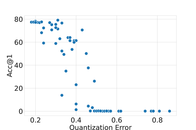
(a) Top 1 accuracy vs. quantization error

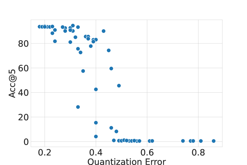
(b) Top 5 accuracy vs. quantization error

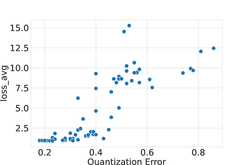
(c) Average model loss vs. quantization error

Figure 1: Relationship between quantization error and model accuracy & loss

Time Complexity Analysis

We analyze the algorithm’s time complexity by considering its two logical components - the error calculations and the bit-width search based on them. Let L be the total number of layers, B the total number of bit-widths, and M the total of QEMs. We calculate the QE of each layer for each bit-width. Thus, the time complexity of MixQuant’s error calculations (line 4-11 in Algorithm 1) is $\mathcal{O}(L*B)$. The bit-width search (line 12-13 in Algorithm 1) compares the QE of each bit-width to the baseline int8 QE for each layer and can be performed for M number of QEMs, which takes $\mathcal{(}L*(B*M))$. Therefore, the overall time complexity is $\mathcal{O}(L*B)+\mathcal{O}(L(B*M))=\mathcal{O}(L(B+B*M))$. This is linear with respect to the number of layers. If we used model loss instead of layer QE to search for optimal bits, we would need to consider all the models generated via the combinations of B number of bit-widths over L number of layers. The time complexity would be $\mathcal{O}(B^{L})$, which is exponential.

5 Results

We implement MixQuant using Python and combine it with two types of quantization techniques: (1) BRECQ [3], a state-of-the-art quantization method, and (2) vanilla asymmetric quantization [12] and evaluate it on the validation set of the Imagenet ILSVRC2012 dataset. Our results demonstrate that MixQuant can optimize the performance of existing quantization techniques.

MixQuant with BRECQ

BRECQ is a state-of-the art quantization method that has been shown to outperform OMSE [4], AdaRound [5], AdaQuant [6], and Bit-Split [7], and in Table 1, we demonstrate in that when MixQuant is combined with BRECQ, we achieve better quantized accuracy than BRECQ alone. Additionally, Table 1 also compares our results with [26], a state of the art mixed precision quantization technique, and shows that the accuracy degradation is significantly greater in [26].

Table 1: Comparison of MixQuant combined with BRECQ, BRECQ, and [26]

	Bits W/A	MixQuant + BRECQ	Bits W/A	BRECQ	Bits W/A	Liu et al. (2021)
ResNet-18	32/32	69.76	32/32	71.08	32/32	74.24
	4, 5, 6/32	70.69	4/32	70.7	4/8	61.68
	4, 5, 6/32	70.69	3/32	69.81	4/8	61.68
	2, 5, 6/32	68.93	2/32	66.3	4/8	61.68
MobileNetV2	32/32	71.88	32/32	72.49		71.78
	4, 5, 6, 7/32	71.92	4/32	71.66	8/8	70.7
	4, 5, 6, 7/32	71.92	3/32	69.5	8/8	70.7
	2, 5, 6/32	59.53	2/32	59.67	8/8	70.7

MixQuant with Asymmetric Quantization

In addition to BRECQ, we combine MixQuant with asymmetric quantization and compare its quantized model accuracy with f32 and int8 baselines. Table 2 shows the set of bit-widths found via MixQuant for various QEMs and various ResNet architectures along with model top-1 and top-5 accuracy. A user can flexibly select the quantization solution based on their requirements with the QEM. For higher QEMs the bit-widths are lower and the model accuracy decreases, while for lower QEMs the bit-widths and quantized model accuracy are higher. Therefore, MixQuant allows its user to flexibly select the trade-off between model accuracy and lowering the quantization bit-width. For example, the highlighted lines in Table 2 satisfy the requirement of selecting the minimum quantization bit-widths such that the model top-1 accuracy degradation is $\leq$ 3%.

Table 2: MixQuant with vanilla asymmetric quantization

Architecture	Experiment	QEM	layers_bit_widths	Top-1 Acc	Top-5 Acc	Avg Loss	QMSE
resnet18	baseline: f32	N/A	all layers are float 32	69.76	89.08	1.25	N/A
resnet18	baseline: int8	N/A	all layers are int 8	69.63	89.07	1.25	N/A
resnet18	MixQuant	2	6, 7	68.20	88.30	1.31	0.23
resnet18		3	5, 6, 7	63.96	85.58	1.51	0.36
resnet18		3.25	5, 6	64.00	85.54	1.51	0.37
resnet18		3.3	4, 5, 6	61.29	83.81	1.64	0.37
resnet18		3.5	4, 6	53.67	77.78	2.04	0.38
resnet34	baseline: f32	N/A	all layers are float 32	73.31	91.42	1.08	N/A
resnet34	baseline: int8	N/A	all layers are int 8	73.24	91.39	1.08	N/A
resnet34	MixQuant	2	6, 7	72.35	90.91	1.12	0.24
resnet34		3	4, 5, 6, 7	61.21	82.93	1.70	0.39
resnet34		3.25	4, 6	61.36	83.05	1.68	0.40
resnet34		3.3	4, 6	61.36	83.05	1.68	0.40
resnet50	baseline: f32	N/A	all layers are float 32	76.13	92.86	0.96	N/A
resnet50	baseline: int8	N/A	all layers are int 8	75.99	92.81	0.97	N/A
resnet50	MixQuant	2	6, 7	75.18	92.52	1.00	0.28
resnet50		3	4, 5, 6	70.58	90.04	1.19	0.43
resnet50		3.25	4, 5, 6	50.13	74.29	2.30	0.45
resnet101	baseline: f32	N/A	all layers are float 32	77.37	93.55	0.91	N/A
resnet101	baseline: int8	N/A	all layers are int 8	77.21	93.51	0.92	N/A
resnet101	MixQuant	1.3	5, 6, 7, 8	76.96	93.42	0.92	0.22
resnet101		1.5	2, 5, 6, 7, 8	59.23	81.74	1.83	0.24
resnet101		1.7	2, 3, 4, 5, 6, 7, 8	58.86	81.05	1.86	0.30
resnet101		1.8	2, 3, 5, 6, 7	52.32	75.61	2.25	0.33
resnet101		1.9	2, 4, 5, 6, 7	49.36	72.63	2.44	0.34
resnet152	baseline: f32	N/A	all layers are float 32	78.31	94.05	0.88	N/A
resnet152	baseline: int8	N/A	all layers are int 8	78.31	94.02	0.88	N/A
resnet152	MixQuant	1.1	7, 8	78.20	94.01	0.88	0.20
resnet152		1.3	6, 7, 8	78.15	94.01	0.89	0.20
resnet152		1.5	5, 6, 7, 8	77.58	93.76	0.91	0.23
resnet152		1.7	3, 5, 6, 7, 8	70.68	90.11	1.22	0.28
resnet152		1.8	2, 5, 6, 7	71.48	90.16	1.19	0.31
resnet152		1.9	2, 4, 5, 6, 7	62.99	85.01	1.66	0.32
resnext50_32x4d	baseline: f32	N/A	all layers are float 32	77.62	93.70	0.94	N/A
resnext50_32x4d	baseline: int8	N/A	all layers are int 8	77.40	93.63	0.95	N/A
resnext50_32x4d	MixQuant	1.3	7, 8	77.43	93.52	0.95	0.19
resnext50_32x4d		1.5	6, 7, 8	77.21	93.51	0.95	0.20
resnext50_32x4d		1.7	5, 6, 7, 8	76.93	93.29	0.98	0.27
resnext50_32x4d		1.8	5, 6, 7	75.43	92.60	1.05	0.30
resnext50_32x4d		1.9	5, 6, 7	75.43	92.60	1.05	0.30
resnext50_32x4d		2	4, 5, 6, 7	72.60	90.79	1.18	0.30
resnext101_32x8d	baseline: f32	N/A	all layers are float 32	79.31	94.53	0.93	N/A
resnext101_32x8d	baseline: int8	N/A	all layers are int 8	79.11	94.51	0.93	N/A
resnext101_32x8d	MixQuant	1.1	7, 8	79.12	94.51	0.93	0.31
resnext101_32x8d		1.3	4, 6, 7, 8	76.61	93.26	1.04	0.33
resnext101_32x8d		1.5	2, 4, 5, 6, 7, 8	59.91	81.46	2.05	0.39
resnext101_32x8d		1.7	2, 4, 5, 6, 7, 8	37.65	59.52	3.84	0.46
resnext101_32x8d		1.8	2, 3, 4, 5, 6, 7	26.14	45.57	5.02	0.49

Runtime Analysis

Table 3 reports the runtime in seconds of MixQuant for various ResNet architectures, where MixQuant considers the bit-widths of 8, 7, 6, 5, 4, 3, and 2, and one or ten different QEMs. It can be observed that the runtime grows with the number of layers since higher number of layers imply a larger search space. For one QEM, the MixQuant search takes between 0.1 and 0.5 seconds. If it is combined with asymmetric per-layer quantization using the optimal bit-widths returned by the search, it takes between 1.0 and 3.2 seconds. If the number of QEMs is increased from one to ten the MixQuant search takes between 0.9 and 5.5 seconds, which represents a linear increase in runtime.

Table 3: Runtime of MixQuant for (a) 1 QEM and (b) 10 QEMs

(a)

Architecture	search	search + quantization
resnet18	0.1 s	1 s
resnet34	0.2 s	1.1 s
resnet50	0.2 s	1.3 s
resnet101	0.4 s	1.7 s
resnet152	0.5 s	2 s
resnext50_32x4d	0.2 s	1.4 s
resnext101_32x8d	0.5 s	3.2 s

(b)

Architecture	search	search+quantization
resnet18	0.9 s	1.8 s
resnet34	1.5 s	2.5 s
resnet50	2 s	3.1 s
resnet101	3.6 s	4.9 s
resnet152	5.2 s	6.8 s
resnext50_32x4d	2 s	3.2 s
resnext101_32x8d	5.5 s	8.2 s

6 Quantization Sensitivity of Weights Ablation Studies

To demonstrate that quantizing DNN weights warrants a search for optimal bit-widths as opposed to uniform precision quantization, we perform two ablation studies to show that different weight layers have different sensitivity to quantization based on their type and position.

Weights Quantization Sensitivity by Layer Type

First, we investigate if different layer types have different sensitivity to quantization. We consider four layer types in the ResNet architecture: (1) first conv layer, (2) conv layers with a 3x3 kernel, (3) conv layers with a 1x1 kernel, and (4) final fully connected layer. For each type of layer, we perform asymmetric quantization and vary its bit-width while keeping the bit-width of all other layer types constant at int8. We calculate the model accuracy, loss, and quantization error for the following quantization bit-widths: 8, 7, 6, 5, 4, 3, and 2.

In Figure 2, we show the impact of varying the bit-width of one layer type at a time on the model top-1 accuracy. Lowering the quantization bit-width of conv layers with a 3x3 kernel has the most adverse impact on top-1 accuracy in shallower ResNet architectures, while in deeper ones it is the conv layers with a 1x1 kernel followed by conv layers with a 3x3 kernel that impacts model accuracy the most. The first conv layer and conv layers with a 1x1 kernel have approximately the same sensitivity to varying bit-width in the shallower architectures. Finally, the quantization bit-width of the final fully connected layer has the smallest impact on model accuracy for all ResNet architectures. In general, starting at 5 bits the model accuracy begins to degrade; however, the deeper architectures are less sensitive to decreasing bit-width. While the reason that the conv layers with a 3x3 kernel and 1x1 kernel are the most sensitive is the fact that those layer types account for the highest number of layers in ResNet, we can still conclude that different layer types have different sensitivity to quantization bit-width measured as the impact on the overall model quality. Therefore, different layer types will benefit from different quantization bit-widths, which motivates MixQuant. Similar results can also be found by measuring layer type sensitivity using the model average loss and quantization mean squared error.

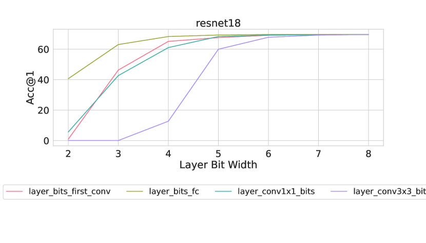
(a) ResNet18

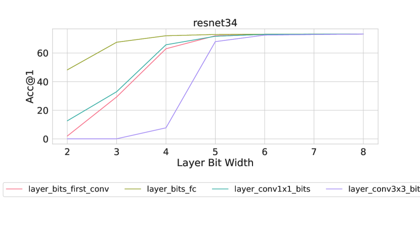
(b) ResNet34

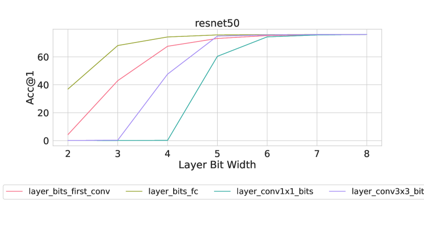
(c) ResNet50

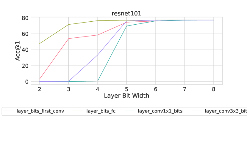
(d) ResNet101

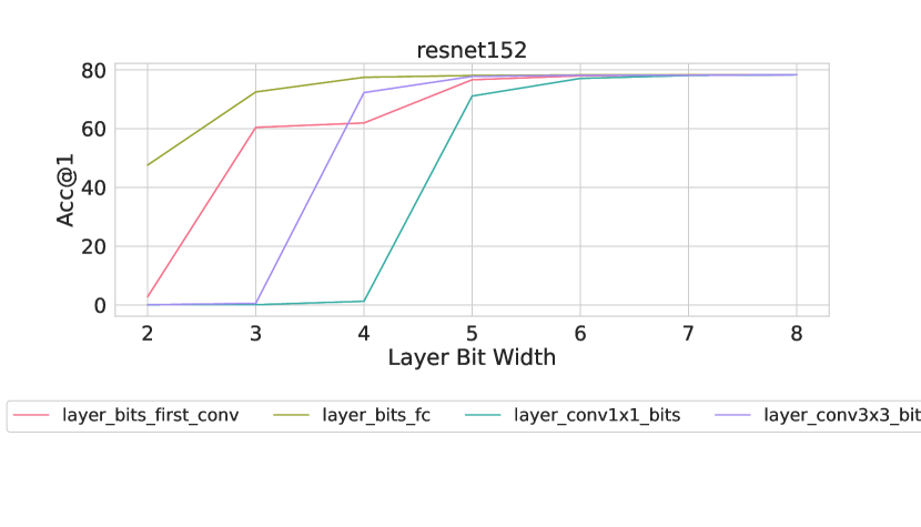
(e) ResNet152

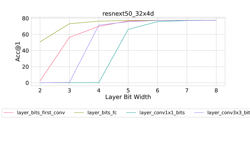
(f) ResNeXt50_32x4d

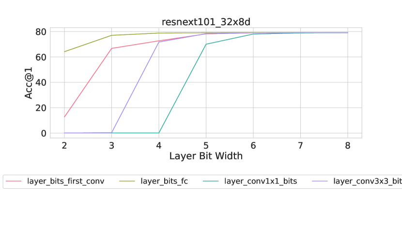
(g) ResNeXt101_32x8d

Figure 2: Sensitivity of different layer types to quantization

Weights Quantization Sensitivity by Layer Position

In addition to the layer type, we investigate if the position of a layer has an impact on quantization sensitivity of weights. We measure the relative quantization error (RQE) of individual layers for the following bit-widths: 8, 7, 6, 5, 4, 3, 2, and define the RQE as $RQE=avg((\vec{f32\,w}-\vec{dequantized\,w})/\vec{f32\,w})$, where $\vec{w}$ is the weights vector and the $avg$ operation returns a scalar that represents the mean of all elements in a vector.

Table 4: The most sensitive layer positions in a DNN measured as a relative quantization error with respect to varying quantization bit-width

Architecture	int8	int7	int6	int5	int4	int3	int2
resnet18	1	1	1	17	17	17	16
resnet34	1	1	20	20	20	33	35
resnet50	46	46	46	46	46	47	44
resnet101	6	6	6	6	97	97	99
resnet152	1	45	45	148	148	148	152
resnet50_32x4d	1	1	1	52	45	45	45
resnet101_32x8d	1	1	49	49	49	96	96

Table 4 identifies the most sensitive layers across various bit-widths and architectures, where layers are indexed from 0 through n, and n equals is the total number of layers minus one. For example, for int8, it is the 1st layer in resnet18 that has the highest relative QE compared to all other resnet18 layers while for resnet50 it is the 46th layer. We can see that the quantization bit-width has a significant impact on the position of the most sensitive layer with the exception of ResNet50. While ResNet50’s most sensitive layer is located towards the end of the network for all bit-widths, other architectures’s most sensitive layer position varies based on the bit-width. For higher bit-widths 8, 7, and 6 it is located at the beginning while for lower bit-widths 2, 3, and 4 it is at the end. The most sensitive layers of ResNet34 and ResNeXt101_32x8d at bit-widths 4, 5, and 6 are in the middle of the network. Based on these experiments, we can conclude that different layer positions have different sensitivity to varying bit-width.

7 Conclusion

In this paper we propose MixQuant, a search algorithm that finds the optimal quantization bit-width for each layer weight and can be combined with any quantization method as a form of pre-processing optimization. We show that combining MixQuant with BRECQ [3], a state-of-the-art quantization method, yields better quantized model accuracy than BRECQ alone. Additionally, we combine BREQ with asymmetric quantization [12] to show that MixQuant has the potential to optimize the performance of any quantization technique. Our code is open-sourced and available at: https://anonymous.4open.science/r/qantizedImagenet-43C5.

References

- [1] Gholami, A., Kim, S., Dong, Z., Yao, Z., Mahoney, M.W., & Keutzer, K. (2021). A Survey of Quantization Methods for Efficient Neural Network Inference. ArXiv, abs/2103.13630.
- [2] Zhou, Shuchang et al. “DoReFa-Net: Training Low Bitwidth Convolutional Neural Networks with Low Bitwidth Gradients.” ArXiv abs/1606.06160 (2016): n. pag.
- [3] Li, Y., Gong, R., Tan, X., Yang, Y., Hu, P., Zhang, Q., Yu, F., Wang, W., & Gu, S. (2021). BRECQ: Pushing the Limit of Post-Training Quantization by Block Reconstruction. ArXiv, abs/2102.05426.
- [4] Choukroun, Y., Kravchik, E., & Kisilev, P. (2019). Low-bit Quantization of Neural Networks for Efficient Inference. 2019 IEEE/CVF International Conference on Computer Vision Workshop (ICCVW), 3009-3018.
- [5] Nagel, M., Amjad, R.A., Baalen, M.V., Louizos, C., & Blankevoort, T. (2020). Up or Down? Adaptive Rounding for Post-Training Quantization. ArXiv, abs/2004.10568.
- [6] Hubara, I., Nahshan, Y., Hanani, Y., Banner, R., & Soudry, D. (2020). Improving Post Training Neural Quantization: Layer-wise Calibration and Integer Programming. ArXiv, abs/2006.10518.
- [7] Wang, P., Chen, Q., He, X., & Cheng, J. (2020). Towards Accurate Post-training Network Quantization via Bit-Split and Stitching. International Conference on Machine Learning.
- [8] Gupta, S., Agrawal, A., Gopalakrishnan, K., & Narayanan, P. (2015). Deep Learning with Limited Numerical Precision. International Conference on Machine Learning.
- [9] Hubara, I., Courbariaux, M., Soudry, D., El-Yaniv, R., & Bengio, Y. (2016). Quantized Neural Networks: Training Neural Networks with Low Precision Weights and Activations. ArXiv, abs/1609.07061.
- [10] Bartan, B., & Pilanci, M. (2021). Training Quantized Neural Networks to Global Optimality via Semidefinite Programming. International Conference on Machine Learning.
- [11] Elthakeb, A.T., Pilligundla, P., & Esmaeilzadeh, H. (2019). Divide and Conquer: Leveraging Intermediate Feature Representations for Quantized Training of Neural Networks. ArXiv, abs/1906.06033.
- [12] Jacob, B., Kligys, S., Chen, B., Zhu, M., Tang, M., Howard, A.G., Adam, H., & Kalenichenko, D. (2017). Quantization and Training of Neural Networks for Efficient Integer-Arithmetic-Only Inference. 2018 IEEE/CVF Conference on Computer Vision and Pattern Recognition, 2704-2713.
- [13] Tailor, S.A., Fernández-Marqués, J., & Lane, N.D. (2020). Degree-Quant: Quantization-Aware Training for Graph Neural Networks. ArXiv, abs/2008.05000.
- [14] Hubara, I., Nahshan, Y., Hanani, Y., Banner, R., & Soudry, D. (2021). Accurate Post Training Quantization With Small Calibration Sets. International Conference on Machine Learning.
- [15] Li, Y., Dong, X., & Wang, W. (2019). Additive Powers-of-Two Quantization: An Efficient Non-uniform Discretization for Neural Networks. International Conference on Learning Representations.
- [16] Nahshan, Y., Chmiel, B., Baskin, C., Zheltonozhskii, E., Banner, R., Bronstein, A.M., & Mendelson, A. (2019). Loss aware post-training quantization. Machine Learning, 110, 3245 - 3262.
- [17] Banner, R., Nahshan, Y., & Soudry, D. (2018). Post training 4-bit quantization of convolutional networks for rapid-deployment. Neural Information Processing Systems.
- [18] Cai, Y., Yao, Z., Dong, Z., Gholami, A., Mahoney, M.W., & Keutzer, K. (2020). ZeroQ: A Novel Zero Shot Quantization Framework. 2020 IEEE/CVF Conference on Computer Vision and Pattern Recognition (CVPR), 13166-13175.
- [19] Chen, T., & Sun, Y. (2019). Differentiable Product Quantization for End-to-End Embedding Compression. International Conference on Machine Learning.
- [20] Kim, S., Gholami, A., Yao, Z., Mahoney, M.W., & Keutzer, K. (2021). I-BERT: Integer-only BERT Quantization. ArXiv, abs/2101.01321.
- [21] Han, Q., Hu, Y., Yu, F., Yang, H., Liu, B., Hu, P., Gong, R., Wang, Y., Wang, R., Luan, Z., & Qian, D. (2020). Extremely Low-bit Convolution Optimization for Quantized Neural Network on Modern Computer Architectures. Proceedings of the 49th International Conference on Parallel Processing.
- [22] Fu, Y., Yu, Q., Li, M., Chandra, V., & Lin, Y. (2021). Double-Win Quant: Aggressively Winning Robustness of Quantized Deep Neural Networks via Random Precision Training and Inference. International Conference on Machine Learning.
- [23] Wang, K., Liu, Z., Lin, Y., Lin, J., & Han, S. (2018). HAQ: Hardware-Aware Automated Quantization With Mixed Precision. 2019 IEEE/CVF Conference on Computer Vision and Pattern Recognition (CVPR), 8604-8612.
- [24] Liang, L. (2020). Post Training Mixed-Precision Quantization Based on Key Layers Selection. ECCV Workshops.
- [25] Wu, B., Wang, Y., Zhang, P., Tian, Y., Vajda, P., & Keutzer, K. (2018). Mixed Precision Quantization of ConvNets via Differentiable Neural Architecture Search. ArXiv, abs/1812.00090.
- [26] Liu, X., Ye, M., Zhou, D., & Liu, Q. (2020). Post-training Quantization with Multiple Points: Mixed Precision without Mixed Precision. AAAI Conference on Artificial Intelligence.
- [27] Lin, D.D., Talathi, S.S., & Annapureddy, V.S. (2015). Fixed Point Quantization of Deep Convolutional Networks. International Conference on Machine Learning.
- [28] Kloberdanz, E., Kloberdanz, K., & Le, W. (2022). DeepStability: A Study of Unstable Numerical Methods and Their Solutions in Deep Learning. 2022 IEEE/ACM 44th International Conference on Software Engineering (ICSE), 586-597.