Outage-Watch: Early Prediction of Outages using Extreme Event Regularizer

Abstract.

Cloud services are omnipresent and critical cloud service failure is a fact of life. In order to retain customers and prevent revenue loss, it is important to provide high reliability guarantees for these services. One way to do this is by predicting outages in advance, which can help in reducing the severity as well as time to recovery. It is difficult to forecast critical failures due to the rarity of these events. Moreover, critical failures are ill-defined in terms of observable data. Our proposed method, Outage-Watch, defines critical service outages as deteriorations in the Quality of Service (QoS) captured by a set of metrics. Outage-Watch detects such outages in advance by using current system state to predict whether the QoS metrics will cross a threshold and initiate an extreme event. A mixture of Gaussian is used to model the distribution of the QoS metrics for flexibility and an extreme event regularizer helps in improving learning in tail of the distribution. An outage is predicted if the probability of any one of the QoS metrics crossing threshold changes significantly. Our evaluation on a real-world SaaS company dataset shows that Outage-Watch significantly outperforms traditional methods with an average AUC of $0.98$. Additionally, Outage-Watch detects all the outages exhibiting a change in service metrics and reduces the Mean Time To Detection (MTTD) of outages by up to $88\%$ when deployed in an enterprise cloud-service system, demonstrating efficacy of our proposed method.

1. Introduction

The use of cloud services for deploying applications has seen a tremendous growth. According to a recent report (clo, 2022), about 94% of enterprises already use cloud services. However, these cloud services, with numerous components, are complex and prone to failures (readitquik, 2023; crn, 2023) and outages (informationweek, 2023b, a) due to frequent updates, changes in operation, repairs, and device mobility. Cloud providers offer services with specific Quality of Service (QoS) requirements, which are technical specifications defining various aspects of system quality, such as performance, availability, scalability, and serviceability. These QoS requirements are driven by business needs outlined in the business requirements. Any failure to meet these predefined QoS standards can lead to Service Level Agreement (SLA) violations, resulting in revenue loss and customer dissatisfaction (Google, 2023b). A study found that a 3-6 day outage by a leading cloud provider in the US could result in $15 billion loss. As a result, cloud system reliability is critical for business success, as outages can severely impact QoS metrics (resource availability, latency, etc.) resulting in compromised system availability and a poor user experience.

Several monitoring and alerting tools (refer §3) are employed to monitor and ensure the performance of cloud services. Automating system troubleshooting has been found to improve reliability, efficiency, and agility for enterprises (Chen et al., 2020a; Dang et al., 2019; Lou et al., 2013). Despite these efforts, cloud systems still experience incidents and outages (Amazon, 2023; Azure, 2023; Google, 2023a). Timely detection and remediation of outages is essential for reducing system downtime. However, a reactive approach to incident detection is often used in practice, hindering effective outage management (Li et al., 2021; Chen et al., 2019a; Zhao et al., 2020b). With a possible innovation in being able to predict the outages well in advance, the time to detect these outages can be reduced significantly.

Consider a real-world scenario in Figure 1 showing the timeline of an outage caused by a flawed configuration change in a Storage service. In this scenario, a 3:54 am (A) failure sparked a sequence of problems, including SQL errors at 4:10 am and an increase in latency that starts affecting the QoS at 4:18 am (B). Alerts were triggered at 5:08 am when latency exceeded pre-defined thresholds. It took nearly 55 minutes (from 4:18 am (B)) to realize it was a cross-service issue and declare an outage at 5:12 am (C). An experienced Site Reliability Engineer (SRE) (Google, 2023b; Atlassian, 2023) was engaged to mitigate the issue, which was resolved at 6:15 am (D) with all services back to normal. Here, the flawed change impacted several SQL databases and spread to other services. The current reactive approach relying on alerts showed significant delay in detecting the outage, as seen by the ramp up in underlying metrics affecting QoS between 4:18 am (B) and 5:12 am (C). This example highlights the potential to predict a substantial fraction of outages in advance by utilizing the information available during the ramp-up phase. In consideration of the strict downtime constraints, with only 500 to 50 minutes of allowable downtime per year corresponding to the uptime guarantees of 99.9% and 99.99% respectively, the early detection of outages, even minutes in advance, can result in significant benefits. The objective of this paper is to present a comprehensive solution aimed at reducing the mean time to detection (MTTD) through early detection of outages.

Outages manifest in two major ways, (i) as degradation in QoS and other metrics, (ii) detected only through user reports and do not manifest in observable metrics. The first type of outages, accounting for 50-70% of the incidents as observed from our data (see §6), exhibit characteristics that allow for prediction. However, outage prediction in cloud systems is a complex task due to the vast number of interdependent metrics. An SRE, who traditionally detect outages using rule-based alerts, often only have a limited view of the overall system, leading to difficulties in quickly and accurately identifying issues. Such approaches rely on human knowledge and is insufficient for large-scale production cloud systems, which have a vast number of complex and ever-changing rules. Our interviews with engineers from various service teams revealed that detection could take hours, particularly in cases where there are multiple concurrent alerts. This highlights the importance of developing a more efficient method for predicting outages in cloud systems.

Previous works (Chen et al., 2019a; Li et al., 2021; Ikram et al., 2022) on failure prediction through runtime monitoring which requires a substantial amount of data from the faulty state of the system are not applicable in this scenario, as outages are rare events (Jus, 2021) and hence, data is not available in the faulty state in plenty. In addition, using alerts to detect outages takes a toll on MTTD since they are fired after a significant ramp-up in metrics has been identified. Failure detection literature from other domains (Anantharaman et al., 2018; Lu et al., 2020) are not extensible to our case since the nature and the quantity of failures is very different in an enterprise service. Our scenario has very few outages and directly extending those works fail.

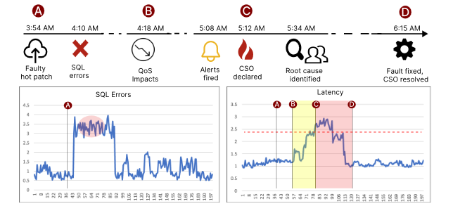
Figure 1. Illustration of the life-cycle of an outage. A refers to the point when the root cause of a fault occurred, B represents the time when it started affecting the performance metrics. When the metrics crossed their respective thresholds, alerts fired which led to an outage being declared at C. The time between C to D is when the engineers diagnose and resolve the issue. The plots below show the variation in the root cause metric and the QoS metric at these times.

In this work, we propose a novel system (Outage-Watch) for predicting outages in cloud services to enhance early detection. We define outages as extreme events where deterioration in the QoS captured by a set of metrics goes beyond control. Outage-Watch models the variations of QoS metrics as a mixture of Gaussian to predict their distribution. We also introduce a classifier that is trained in a multi-task setting with extreme value loss to learn the distribution better at the tail, thus acting as a regularizer (Schölkopf and Smola, 2002). Outage-Watch predicts an outage if there is a significant change in the probability of the QoS metrics exceeding the threshold. Our evaluation on real-world data from an enterprise system shows significant improvement over traditional methods with an average AUC of 0.98. Furthermore, we deployed Outage-Watch in a cloud system to predict outages, which resulted in a 100% recall and reduced MTTD by up to 88% (20 - 60 minutes reduction).

Our major contributions can be summarized as follows:

1. We propose a novel approach Outage-Watch to predict outages in advance, which are manifested as large deteriorations in a chosen set of metrics (QoS) reflecting customer experience degradation. Outage-Watch works even in the absence of actual outages in training data.

2. Outage-Watch generates the probability of a metric crossing any threshold, making it flexible to define the threshold, unlike classification tasks. It predicts the distribution of QoS metric values in future given current system state, and improves learning the tail distribution via extreme value loss to capture outages before they happen.

3. An evaluation of the approach on real service data shows an improvement of $7-15\%$ over the baselines in terms of AUC, while its deployment in a real setting was able to predict all the outages which exhibited any change in the observable metrics, thus reducing the MTTD.

The rest of the paper is organized as follows. We briefly talk about related works in Section 2 followed by the background and problem formulation in Section 3. In Section 4 and 5 we outline the motivation and describe Outage-Watch. With Section 7 analyzing its performance, we conclude in Section 8.

2. Related Work

Service reliability has been a well-researched area in both academia and industry (Chen et al., 2019a; Li et al., 2021; Ikram et al., 2022; Chakraborty et al., 2023a; Chen et al., 2016). Several works have attempted to address the problems of detecting, localizing, and mitigating outages and failures. Alerts are often used in detecting outages (Lin et al., 2014; Jiang et al., 2009; Zhao et al., 2020c), which are triggered when a system fault occurs and metric values crosses a threshold. Recent approaches such as AirAlert (Chen et al., 2019a), Fog of War (Li et al., 2021), and eWarn (Zhao et al., 2020b) compute features based on alerts and predict outages using tree-based models. However, alerts only trigger when a system is already in a critical state, thus incurring low reduction in MTTD.

Previous research in the area of time series forecasting constitutes a relevant body of literature since changes in metric value time series can be forecasted to detect outages. Classical auto-regressive models (Gurland, 1954; Adhikari and Agrawal, 2013) to predict future metric values have limitations that have been overcome by recent advancements in deep neural network (DNN) based models, such as RNNs, LSTMs and GRUs, which have proven to be more effective in modelling time series data (Siami Namini et al., 2018; Dasgupta and Osogami, 2017; Yang et al., 2015; Lin et al., 1996; Hochreiter and Schmidhuber, 1997; Cho et al., 2014). Empirical evidence supports the use of these deep recurrent models for time series prediction (Lin et al., 2017b; Qin et al., 2017; Zhu et al., 2017). However, they perform poorly (Laptev et al., 2017) in predicting rare events like outages due to imbalanced data (Laptev et al., 2017; Lin et al., 2017a), also known as extreme events (Albeverio et al., 2006; Ghil et al., 2011). Predicting extreme events remains a challenging and active area of research (Friederichs and Thorarinsdottir, 2012; Haan and Ferreira, 2006).

Recent studies (Laptev et al., 2017; Ding et al., 2019) have attempted to address the challenge of forecasting extreme events in time series data through innovative DNN architectures. (Laptev et al., 2017) employs an auto-encoder for feature extraction while (Ding et al., 2019) uses an Extreme Value Loss (EVL) function. However, modelling point prediction of extreme events as classification task would need re-estimation of the model if the threshold definition changes for defining such events. However, Outage-Watch sets itself apart by combining the EVL function with LSTM and predicting the future distribution of events using a mixture normal network, thus allowing a flexible change of threshold.

In the domain of reliability engineering, prior studies have concentrated on detecting anomalies in time series data for monitoring systems (Chen et al., 2022). Supervised anomaly detection models like (Chen et al., 2019b; Park et al., 2019; Li et al., 2021) are effective in predicting anomalies, but they require a substantial amount of labelled data, making them unsuitable for our application. On the other hand, unsupervised methods (Zhang et al., 2019) can be used to identify anomalies in data without the need for labelled data. More recently, ML-based models including autoencoders and transformers are used for anomaly detection in seasonal metric time series (Tuli et al., 2022; Su et al., 2019; Park et al., 2018). However, they are limited to detecting events as they happen and lack interpretability to distinguish significant service degradation. Our approach differs by predicting the probability of metric exceeding threshold through its probability distribution analysis, instead of simply detecting whether the actual metric crosses a threshold or not, as in traditional anomaly detection.

In related literature of failure detection, several efforts have been made to predict specific types of failures, utilizing large sets of system logs and metrics (Zhang et al., 2018; Oki et al., 2018; Xu et al., 2018). Our approach differs in predicting general incidents based on a limited set of relevant metrics, determined by domain knowledge. Previous works like (Anantharaman et al., 2018; dos Santos Lima et al., 2017; Lu et al., 2020) have used ML and DNN techniques to predict disk failures. A comparison of disk failure prediction methods was presented in (Lu et al., 2020). However, they are not suitable for predicting rare and extreme outages. Our approach, based on distribution forecasting, is flexible and outperforms some of the baselines discussed in (Lu et al., 2020).

3. Background and Problem Definition

In this section, we briefly describe basic monitoring system concepts, followed by the problem formulation.

Monitoring Metrics: In any enterprise level service deployment, reliability engineers monitor the performance of these deployed services. Various monitoring tools like grafana (gra, 2023), new-relic (new, 2023), splunk (spl, 2023), etc. are employed to monitor the services and collect service metrics that can be used to measure the performance of the system. Monitoring metrics provide the most granular information, with these tools recording them at specific time intervals.

Alerts: Alerts are defined on monitoring metrics. Whenever these metrics cross a certain pre-defined threshold defined by the reliability engineers, an alert is triggered. They represent system events that require attention, such as API timeouts, exceeding response latencies, service errors and network jitters. An alert contains several fields like the alert definition, time of alert, which service fired the alert, text description of the alert, datacenter region where the alert was fired and severity level which can be ”high”, ”medium” or ”low”.

Extreme Events: An extreme event is characterized by a set of monitoring metrics exceeding their respective thresholds (95%-ile metric threshold based on our data), causing unusual system behaviour. This results in multiple alerts with varying levels of severity being triggered, prompting engineers to take action. It’s important to note that not all extreme events lead to outages, as they may not necessarily indicate a fault in the system. Extreme events which lead to outages cause violations in Service Level Agreements (SLAs). Extreme events can be perceived as situations when the system starts showing signs of degradation, and the metric values surpass their 95 or 99%-ile thresholds. In addition, it is important to note that extreme events are not recorded as separate incidents. We generate proxy labels (see §5.1.3) to identify the extreme events.

Outage: In general, outages are declared under severe situations, when extreme events persist for a long time, leading to a degradation in the service quality and often leading to a customer impact. Often, outages affect multiple services where a fault propagates based on service dependency. Mitigating outages require cross-team collaboration. An outage usually triggers correlated alerts (Chen et al., 2020b; Zhao et al., 2020a) and escalates from a single or a group of alerts. Not all extreme events manifest as an outage since engineers manage these systems through constant monitoring, and they identify and intervene in the system during potential issues even before they escalate into full-scale outage.

3.1. Problem Formulation

We now formally define our problem statement. Metrics $\mathcal{M}_{tot}$ are continuously monitored in the system, essentially forming a time series. The task is to understand the trends in some or all of the metrics in $\mathcal{M}_{tot}$ and predict an impending outage, with the goal of predicting it as early as possible. It is obvious that a change in the metrics will show up only when a fault has occurred. Thus, the goal of an outage forecasting solution is to minimize the lag time between the actual occurrence of the fault and its identification as an extreme event, while also minimizing false positive cases.

With $t$ as the wall-clock time, the input to the outage forecasting module is a set of relevant metrics (see §5.1.1) from $[t-w,t]$ where $w$ is the window length. More details on the pre-processing of metrics is elucidated in §5.1.2. With ground-truth labels generated based on the occurrence of extreme events, the supervised ML model Outage-Watch aims to forecast an outage by learning the distribution of the relevant metrics at a certain time in the future. A distribution of metrics is essentially a probability density function of the metric values at a certain time.

4. Solution Motivation

In this section, we present the rationale behind our solution design and provide a concise overview of how it functions.

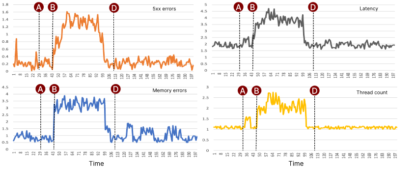
Figure 2. Multiple performance metrics, some of which are QoS metric gets impacted during an outage. The collective information from all these metrics help in detecting the outage. A, B and D corresponds to the time defined in Fig. 1

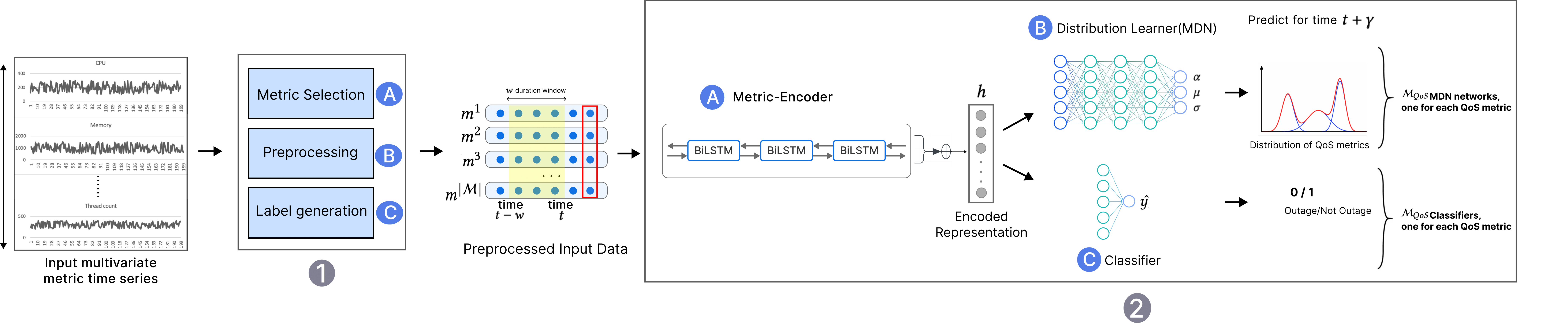
Figure 3. Overall Architecture of Outage-Watch, comprising of (1) metric processing phase and the (2) distribution learning phase. The distribution and label prediction generated from (2) at time step $t$ are evaluated against ground-truth metric value and labels from a future time step $t+\gamma$, which we get from (1B) and (1C) respectively.

4.1. Design Motivation

As discussed in §1, outage prediction models should aim to predict the probability of an outage in advance to ensure timely recovery during a fault. One way to achieve this is to monitor the system metrics for deviations from their regular trend, as these deviations are often indicative of an outage. However, the current system monitoring tools often fail to detect deviations until they surpass a specific threshold and activate an alert, provided that an alert has been defined for those system metrics. However, proactive monitoring of system metrics allows for earlier and more efficient identification of outages. This motivates the design of our proposed approach, Outage-Watch.

We have observed from the data (Figure 2) that during an outage, multiple metrics (Ana, 2016) show disturbances and deviations from trends simultaneously. These metrics progressively become more extreme and affect multiple interdependent services. Outage-Watch takes multiple monitoring metrics as input and aims to predict the future behaviour or change in the values of certain metrics (which we refer to as Quality of Service (QoS) metrics, and will be further defined in §5.1.1). By predicting the distribution of these metrics in advance, we can compute the probability of an upcoming outage based on the likelihood of the metric value crossing a certain threshold. These thresholds can be dynamic and may be defined by Service Level Agreements (SLAs) on QoS metrics for each service.

Why do we need to learn the distribution of metrics? Outages are often scarce in any established production-level service. Hence, if the outage prediction task is modelled as a simple classification problem, a machine learning model will tend to fail even after the imbalance in the dataset is addressed, because of the extremely skewed distribution of data points coming from one class (outage occurrences). For example, it is often the case that one observes only two outages over a period of 6 months. However, one way to circumvent this issue is to design our problem as a distribution learning task. We then have a corresponding metric value at every timestamp of the data, and a learned regression model can predict a metric value at any other time stamp. We can also use the same strategy to learn a more accurate distribution in the tail, where extreme events are often manifested. This allows the flexibility of constructing the entire distribution and using variable threshold based on Service Level Agreements (SLA) requirements.

We provide further technical details on how the model predicts the distribution of the relevant metrics and how it can be used to predict outages in subsequent sections.

4.2. Architecture Overview

The proposed framework of Outage-Watch (Fig. 3) comprises two main phases: a metric processing phase (denoted as in Fig. 3 and a distribution learning phase (denoted as in Fig. 3). Module first selects the relevant metrics that will be used to forecast the outages, pre-processes them and then generates proxy labels. What we mean by labels here and why do we need to generate them will be elucidated in details in §5.1.3. On the other hand, module forecasts the outage by predicting the distribution of the relevant metrics selected from phase at a future time.

In order for the distribution learner to predict outages at a future time $t+\gamma$ where $\gamma$ is the prediction look-ahead, the machine learning algorithm must learn from the appropriate ground truth. Thus, with input data at $t$, the ground truth is constructed such that our method can predict the distribution of the metrics at time $t+\gamma$ and hence predict potential outages. The distribution learner framework first uses a metric encoder to encode the system state in the past trend of monitoring metrics, and then the distribution of the relevant metrics is forecasted using a Mixture Density Network (MDN). MDN aims to predict the parameters of the forecasted distribution. Additionally, the framework uses a classifier as an extreme value regularizer for better learning in the tail of the distribution. The technical details are presented in §5.2.

Though the pipeline is trained to predict the parametric distribution of metrics, inference on whether and when the outage is being detected need to be developed. §5.4 focuses on identifying the likelihood of outages by evaluating the probability of each of the relevant metric crossing a defined threshold. If there is a sudden increase in the probability of exhibiting extreme values based on the distribution learnt, Outage-Watch takes this as an indication of an outage. A thresholding mechanism is employed on the probability value to predict an outage.

5. Outage-Watch

In §4.2, we have discussed the overall architecture of Outage-Watch and talked about its two main components briefly. We shall now delve into the details of each component.

5.1. Metric Processing

5.1.1. Metric Selection and Quality of Service (QoS) Metrics (Fig. 3[1A])

The monitoring tools collect a large set of service metrics $\mathcal{M}_{tot}$ for a system. However, many such metrics recorded by these tools are often never used by the SREs (Met, 2019). Also, storage and handling of metrics data is non-scalable and gets expensive over time. Consequently, we derived a condensed subset of metrics, denoted as $\mathcal{M}$. In our specific scenario, we filtered down the number of metrics from $\sim$2000 in $\mathcal{M}_{tot}$ (Met, 2023) to 42 using a step-wise procedure.

We employed established techniques (Pudjihartono et al., 2022) for feature selection process. Firstly, features were filtered using correlation analysis and rank coefficient tests. Then, time series features that were constant throughout the time series or exhibited low variance were omitted due to their limited informational value. To refine our feature set further, we incorporated domain-specific knowledge: retaining only those metrics that either trigger alerts or have been emphasized in previous outage analysis reports that are generated post-identification and mitigation of outages by engineers. This process yielded a focused feature set well-suited for effective service monitoring and analysis.

However, only a fraction of $\mathcal{M}$ directly reflects the service quality as perceived by the customer, for example, latency of a service, number of service failure errors, resource availability, etc. These metrics, known as Quality of Service (QoS) metrics $\mathcal{M}_{QoS}$ or the golden metrics (Beyer et al., 2016), are used by the SRE to define outages. These metrics are crucial to monitor because cloud service providers face revenue loss if QoS is not met due to violations of Service Level Agreements (SLAs). Based on the alert severity used by the SRE team and the SLA definitions, we select five golden metrics comprising of (i) Workload, (ii) CPU Utilization, (iii) Memory Utilization (iv) Latency, and (v) Errors. These metrics are often used for system monitoring in industries and have been utilized in prior works (Li et al., 2022; Chakraborty et al., 2023b). The golden signals can often refer to different metrics based on service components. For example, the latency metric refer to disk I/O latency for storage service, web transaction time for web services, query latency for databases, etc.

Outage-Watch uses the entire set of metrics $\mathcal{M}$, to forecast the likelihood that $\mathcal{M}_{QoS}$ metrics will surpass a threshold in the future. We do not specifically forecast the likelihood of metric values of $\mathcal{M}\setminus\mathcal{M}_{QoS}$ crossing the threshold since these capture small issues which propagates within the system and gets manifested into the QoS metrics. Also, QoS metrics capture the user impact directly. It should be noted that our choice of $\mathcal{M}_{QoS}$ is based on system domain knowledge which we gathered from the inputs from reliability engineers on the most important metrics that define an outage. Nonetheless, our approach will work in the same way for a different set of $\mathcal{M}_{QoS}$ metrics.

5.1.2. Pre-processing (Fig. 3[1B])

After the selection of metrics $\mathcal{M}$, we handle the missing values differently for different category of metrics. For some metrics, a missing value might indicate a null value, which can be replaced with a zero. For other metrics, the rows containing missing values may be dropped. For example, if there are missing values in a metric that defines an error, these can be replaced with zeroes, as this indicates that there were no errors in the service. However, if there are missing values in utilization-based metrics, it may be necessary to drop those rows, as the missing values could be due to a fault with the monitoring system. Once the missing values are handled, each metric $m^{i}$ is normalized using Equation 1.

(1) $$m^{i}=\frac{m^{i}-min(m^{i})}{max(m^{i})-min(m^{i})+\epsilon}$$

Following this, we create a time series of $\mathcal{M}$ metrics with a rolling-window of size $w$. That is, for each time instant $t$ and metric $m^{i}\in\mathcal{M}$, we create a time series $m^{i}_{w}=\{m^{i}_{t-w},\ldots,m^{i}_{t}\}$, where $m^{i}_{t}$ refers to the value of the metric $m^{i}$ at $t^{th}$ time instant. We thus create $X=\{m^{1}_{w},m^{2}_{w},\ldots,m^{|\mathcal{M}|}_{w}\}$, which forms a sequence of metric values that can be used as an input to our encoder model.

5.1.3. Label Generation (Fig. 3[1C])

In real-world production services, outages are rare due to the robust deployment architecture and constant monitoring system in place. SREs often intervene to prevent the full-scale outages resulting in a rarity of such events. However, these potential issues when interventions are performed can still be considered as extreme situations (see §3), which will allows us to better understand the system’s behaviour and predict critical issues in advance. Thus, instead of having the time periods when an outage was actually declared as the ground truth, we modify our definition of labels to the time periods of extreme events. Such modifications facilitate us in forecasting the distribution of the relevant metrics. However, the challenge of labelling the data during these extreme events remain. To address this issue, we perform the following algorithmic steps that incorporates domain knowledge to generate proxy labels for outages or extreme situations.

1. Take ${w^{\prime}}$ minutes windows for each of the metrics ${m}_{i}$ from the set $\mathcal{M}_{QoS}$.

2. Select those windows where the value of ${m}_{i}$ crosses a percentile threshold $\mathcal{T}$ for at least $\alpha$ fraction of $w^{\prime}$ window.

3. Filter the previously obtained time windows by keeping only those where at least k alerts were fired in the system.

These chosen time windows serve as proxy labels for extreme events. Here, we take $w^{\prime}$ as 10 minutes, $\mathcal{T}$ as 95, $\alpha$ as $0.5$, k as 1.

These steps indirectly incorporate domain knowledge to accurately generate labels for outages and extreme situations using alerts defined by SRE. This process not only allows us to create a denser labelling of extreme events, which can aid in the prediction of potential outages or situations that could have escalated to an outage in advance, but it also includes some less severe cases, which can aid in model training recall. The proxy labels serve as positive training samples for the model.

5.2. Distribution Forecasting

Through this module, Outage-Watch aims to learn how the QoS metrics will behave in a future time to forecast the probability of an outage. We outline the component details below.

5.2.1. Metric-Encoder (Fig. 3[2A])

Before we can learn the distribution of QoS metrics, we must encode the past behaviour of the service metrics which captures the system state as a latent vector representation. Metric-Encoder extracts information via ML technique to encode spatial as well as temporal relation (Shao et al., 2020) between the metrics. Spatial correlation captures how each behaviour of metric $m^{i}\in\mathcal{M}$ affects the QoS metrics $\mathcal{M}_{QoS}$, while the temporal dependence captures the time series trend in $X$. Though both statistical and ML-based techniques have been studied in this regard (Chatfield, 2000; Hyndman and Khandakar, 2008; Lim and Zohren, 2021; Torres et al., 2021), it has been shown that ML-based models, and especially Recurrent Neural Network (RNN) models outperform conventional methods (Siami Namini et al., 2018) in encoding a time series due to their ability to capture sequential dependencies and temporal patterns in data. Several RNN-based models like Long Short-Term Memory (LSTM) (Hochreiter and Schmidhuber, 1997) or Bidirectional LSTM (BiLSTM) (Graves and Schmidhuber, 2005; Schuster and Paliwal, 1997) models can be used for our purpose. Based on our experimental results with various RNN architectures (see §7.1.1), we choose BiLSTM as the metric encoder model.

LSTM uses gating mechanism to control information encoding, while the hidden state ($h_{t}$), a multi-dimensional vector, maintains the encoding of the input time series. BiLSTMs extend LSTMs by applying two LSTMs, one forward and one backward, to input data to capture information from both directions. The Metric-Encoder takes $X$ as input and outputs a vector representation ($h$) capturing the temporal and spatial relationship of the metrics.

5.2.2. Multi-Task Learning

We propose a multi-task learning (Ruder, 2017; Caruana, 1997) problem, where one task is to learn the distribution of each QoS metric $y\in\mathcal{M}_{QoS}$ from the Metric-Encoder output, while the other task classifies the Metric-Encoder output as an outage or not. We now describe each of the task in detail.

Task 1: Distribution Learning (Fig. 3[2B]). The first task aims to learn a parametric distribution governing the QoS metrics conditional on the encoded system state representation. More precisely, given a time series of metrics $X$ which was encoded to form a vector $h$, we wish to estimate the probability of a metric $y\in\mathcal{M}_{QoS}$ given $X$, $p(y|X)$. Learning a distribution is essentially learning the parameters governing it. In general, the metric $y$ is often assumed to follow a normal distribution $\mathcal{N}(y;\mu,\sigma)$, since we observe limited data points in the tail of the distribution. However, in a real production system, a normal distribution might underfit the actual data distribution. Often, we don’t necessarily have simple normal distributions. To overcome this limitation, we estimate the distribution of the QoS metric via a mixture of normal distributions with $C$ mixture components, where the probability distribution of a metric $y$ given $X$ is of the form:

(2) $$p(y|X)=\sum_{c=1}^{C}\alpha_{c,y}(X)\mathcal{N}(y|\mu_{c,y}(X),\sigma_{c,y}(X)),$$

where $c$ denotes the index of the corresponding mixture component, and $\alpha_{c,y}$ is the mixture proportion representing the probability that $y$ belongs to the $c^{th}$ mixture component $\mathcal{N}(y|\mu_{c,y},\sigma_{c,y})$.

It is well known in the literature that a mixture of Gaussian/normal distributions is capable of modelling any arbitrary probability distribution with correct choice of $C,\alpha_{c},\mu_{c}$ and $\sigma_{c}$ (Reynolds, 2009). We aim to estimate a mixture distribution for each QoS metric $y$ via a separate Mixture Density Network (MDN), that comprises a feed-forward neural network to learn the mixture parameters $\mu_{y},\sigma_{y}$ and the mixing coefficient $\alpha_{y}$. We have chosen $C=3$ after experimental analysis (see Fig. 6(a)), and hence each MDN has 3 values of $\alpha_{y},\mu_{y}$ and $\sigma_{y}$. The network is learnt through minimizing the negative log-likelihood loss of obtaining the ground truth metric value of $y$ given the mixture distribution, averaged over all metrics $\mathcal{M}_{QoS}$. Formally,

(3) $$\operatorname*{arg\,min}_{\theta}l(\theta)=-\frac{1}{|\mathbb{R}|}\operatorname*{\sum}_{X,y\in\mathbb{R}}\log p(y|X)$$

Here $\mathbb{R}$ corresponds to the realm of possibilities. MDN hence learns the parameters of the distribution of QoS metrics, which can then be further used to compute the probability of $y$ crossing a certain threshold to predict outages.

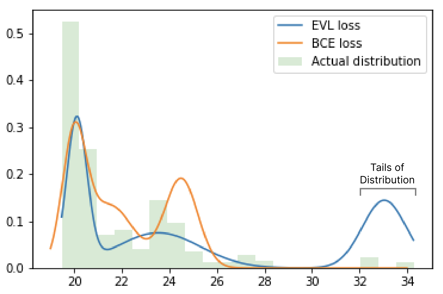
Figure 4. Using Extreme Value Loss in the classifier over BCE can aid the distribution learner to learn a better distribution at the tail.

Task 2: Outage Classification (Fig. 3[2C]). We have observed through experiments (see §7.1.3) that the distribution learnt by MDN performs poorly at the tail, where extreme values are generally observed and can be used to forecast outages (Figure 4). To overcome this limitation, a feed-forward neural network performs outage classification in a multi-task setting, where we predict whether an outage will happen or not from the encoded output from the Metric-Encoder. We use the output proxy labels generated in §5.1.3 as a ground truth.

This module acts the extreme value regularizer. where the intuition is that the synthetically generated proxy labels will act as a regularizer for better learning in the tail of the distribution. Similar to distribution learning, we have separate neural networks for each QoS metric in $\mathcal{M}_{QoS}$.

To classify outages, we have used the Extreme Value Loss (EVL) (Ding et al., 2019; Coles et al., 2001), which is a modified form of Binary Cross Entropy (BCE) Loss as the loss function. EVL reduces the number of false positives by assigning more weight to the penalty of incorrectly predicting outages. EVL works well with imbalanced data as we have observed through experiments. EVL can be formally defined as,

(4) $$\mathbb{L}_{EVL}=-\frac{1}{N}\sum_{i=1}^{N}\beta_{0}\left[1-\frac{\hat{y_{i}}}{\delta}\right]^{\delta}y_{i}\log{\hat{y_{i}}}+\\ \beta_{1}\left[1-\frac{1-\hat{y_{i}}}{\delta}\right]^{\delta}(1-y_{i})\log{(1-\hat{y_{i}})},$$

where $N$ is the size of the batch, $y_{i}\in\{0,1\}$ is the ground-truth value and $\hat{y_{i}}$ is the value predicted by our model Outage-Watch, $\beta_{0}$ is the proportion of normal events in the batch and $\beta_{1}$ is the proportion of extreme events in the batch. We use $\delta=2$ in the loss function for the experiments.

5.3. Training

Since we want to predict the probability of an outage in advance and reduce the MTTD, the ground truth metric values and the proxy labels should also correspond to a future time $t+\gamma$. Thus, at a time $t$, the Metric-Encoder takes $X$ which is a time series of all metric values from $t-w$ to $t$ as input. The ground truth value for Task 1 is the metric value for each QoS metric $y$ at time $t+\gamma$ and while for Task 2, we use the proxy label (see §5.1.3) computed from the QoS metric values at $t+\gamma$. We train the entire pipeline consisting of the Metric-Encoder, mixture density network and the classifier in an end-to-end fashion.

It should also be noted that with a large $\gamma$, one can aim to predict an outage well in advance, but the distribution followed by the QoS metric will not be accurate. Hence, a careful selection of $\gamma$ is necessary. By our experiments (see Fig. 6(b)), we show that $\gamma=10$ mins works the best for our purpose.

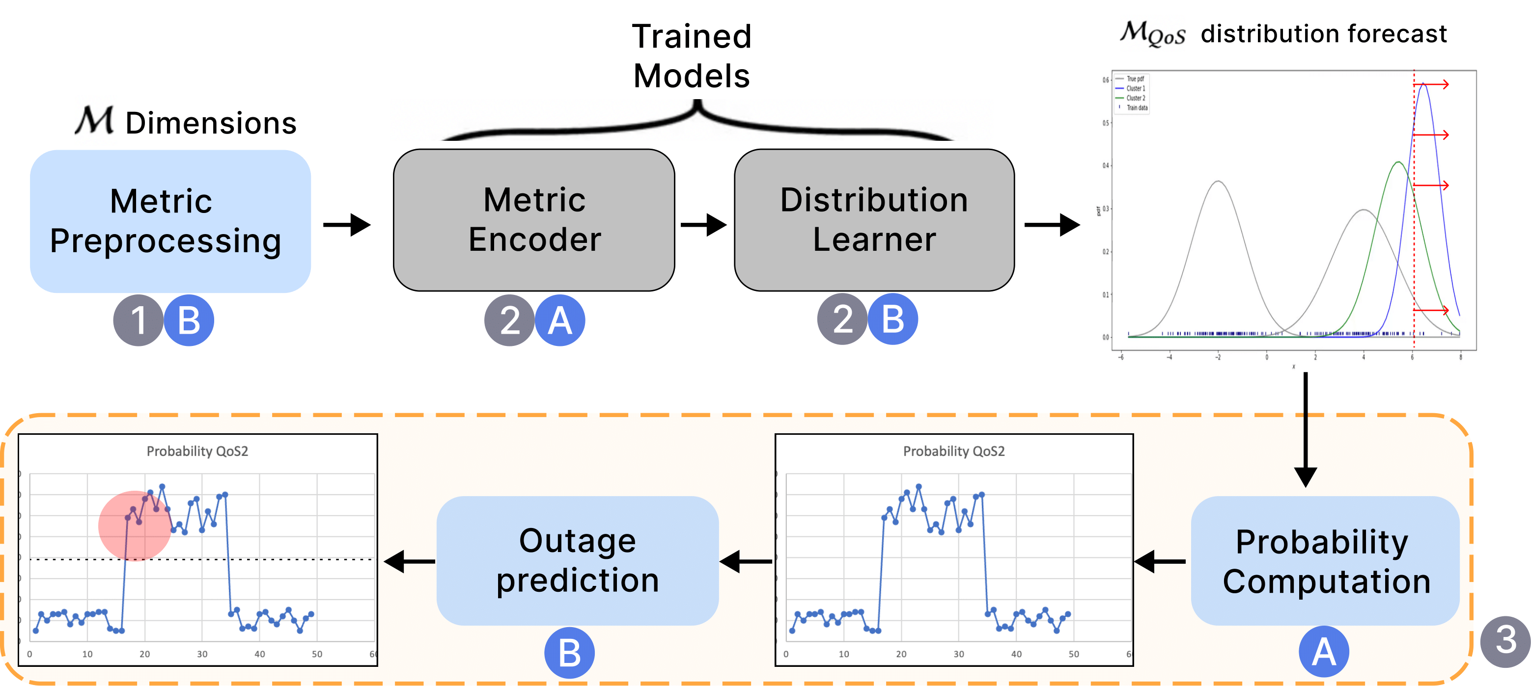
Figure 5. Tasks performed during inference time to predict potential outages from the predicted distribution

5.4. Inference

At inference time, we predict and use only the distribution of the QoS metrics, while excluding the classifier from our inference pipeline to predict an outage. The distribution of the QoS metrics provide us with more flexibility and enables us to define outages based on custom thresholds. Moreover, the distribution captures the entire spectrum and specifically the tail metric values. However, the steps to predict an outage from the distribution of the QoS metrics can be summarized as below.

5.4.1. Probability Computation (Fig. 5[3A])

We first compute the probability of an outage occurring by computing the probability that the value of the QoS metric crosses a pre-defined threshold. These thresholds are generally defined by the SLAs that have been agreed with a particular customer. As an example, an agreement of achieving a service latency of at most $\rho$ milli-seconds for 99% of the times might have been signed with the cloud service provider, and can be termed as an SLA. Hence, in this case, the threshold is 99%. Formally, the probability of a QoS metric value $y$ crossing a threshold $\mathcal{T}$, and hence the probability of an outage occurring can be defined as

(5) $$Prob(Outage)=\sum_{c=1}^{C}\alpha_{c}[\mathcal{N}(y|\mu_{c},\sigma_{c})>\mathcal{T}]$$

5.4.2. Outage Prediction (Fig. 5[3B])

From the probability computed above, we use a thresholding technique on $Prob(Outage)$ to predict the outages. We compute the threshold based on Youden’s J Index (Youden, 1950) on training data. It is a popular thresholding technique for imbalanced data (extreme events are very few as compared to the usual metric values), which uses the Area under the ROC curve (AUC) to compute the threshold. On the training data containing the proxy labels and the corresponding probability of an outage occurring, Youden’s J Index tries to compute the threshold such that it increases the precision and recall. We maintain the same threshold for all our evaluations.

6. Implementation Setup

In this section, we outline the experimental process and the setup we followed. We have implemented Outage-Watch in python and used tensorflow (Abadi et al., 2016), a standard open-source library to implement the ML models. We have run Outage-Watch on a system having Intel Xeon E5-2686 v4 2.3GHz CPU with 8 cores.

Source of Data: The data is sourced from a prominent SaaS enterprise offering extensive software and digital services. It leverages Amazon Web Services (AWS) and Microsoft Azure for cloud provisions. The software infrastructure covers diverse domains including programming languages, databases, AWS, Azure, Docker, Kubernetes, Jenkins, and more.

Dataset: We collect the dataset for evaluating Outage-Watch from a real-world service hosted by a large cloud-based service provider. The metrics data was obtained through a message queue pipeline deployed on the monitoring system of the service. We have collected a total of 3 months of metrics and outage data from the monitoring system for training and testing purposes where data from the last 3 weeks were used for testing. We collected $\sim$2000 metrics, which was reduced to 42 as discussed in §5.1.1. Outages have a widespread impact within the enterprise affecting multiple services. Since there were no outages observed during the period of the training data while one outage was observed during the period of test data, we generated time periods when the extreme situations occurred (see §5.1.3). It amounted to around 5-7% of the total training data, thus exhibiting a skewed label imbalance.

Model Hyperparameters: The implementation details for the ML models used in Outage-Watch (§4.2) are outlined as follows. The BiLSTM model in the Metric Encoder has 128 hidden units ($h=128$), followed by a dropout layer with $p=0.2$. Regularization techniques were used while training the model to prevent overfitting. The feed-forward Mixture Density Network (MDN) which models the distribution parameters of QoS metrics has two hidden layers with 200 neurons each, with ReLU (Glorot et al., 2011) activation function in the hidden layers. The neuron outputting the mixing factor of components ($\alpha$) use a softmax function. The classifier feed-forward network has one hidden layer with 20 neurons with ReLU activation, while the output layer use the sigmoid function. We use a learning rate of 0.001 with the Adam optimizer for training.

Baselines: The baselines for evaluation are chosen following an approach similar to the work presented in (Lu et al., 2020). We leverage some of the fundamental classification and regression techniques for outage prediction. It includes Naive Bayes classifier, random forests and gradient boosted decision trees. Naive bayes is a probabilistic machine learning model while the other two are ensemble methods that are constructed using a multitude of individual trees. We implement these baselines to use them as a proxy for prior learning based outage prediction models. We also use a BiLSTM classifier as a baseline, which uses only classifier network on the encoded BiLSTM representation to predict outages.

Evaluation Metrics: To evaluate the effectiveness of various approaches, we use AUC-PR and F1 score. AUC-PR calculates the area under the precision-recall (PR) curve and is commonly used for heavily imbalanced datasets (Sofaer et al., 2019) where we are optimizing for the positive class (outage being detected) only. AUC-PR is computed using the probability of an outage occurring or not (from Equation 5). Also, based on the probability values, we use the procedure in §5.4.2 on training data to compute a threshold for detecting outages, which we use to compute the F1 score in test data.

Other Hyperparameters: For all the experiments, we choose a window $w=60$ mins to create a windowed time series of metric data. On the contrary, we vary the prediction look-ahead $\gamma$ from 5 mins to 30 mins. In §7.1.4, we experimentally show the optimal value of $\gamma$. Unless specified, we maintain threshold $\mathcal{T}=95\%$ (Eq. 5) for all the experiments.

7. Evaluation

In this section, we present the experimental results and aim to address the following research questions:

• RQ1: How do our design decisions align with the ablation studies performed?

• RQ2: How does our approach compare to the established baselines?

• RQ3: How does our approach perform in a real-world cloud deployment scenario?

7.1. Design Choices (RQ1)

7.1.1. Metric Encoder Model

In §5.2.1, we claim to use Bidirectional LSTM (BiLSTM) as the model for metric encoder. In this subsection, we discuss the experiments conducted to determine the optimal architecture and the rationale behind using BiLSTM. We conducted experiments using four different types of RNNs: LSTM (Hochreiter and Schmidhuber, 1997), BiLSTM (Graves and Schmidhuber, 2005), Stacked LSTM (Cui et al., 2018), and Stacked BiLSTM (Cui et al., 2018). The encoded representation was then used to forecast the distribution in a multi-task setting with EVL in the classifier network. The performance of each architecture was evaluated using AUC-PR metric. We have experimented with varying values of $\gamma\in\{5,10,15,30\}$ min. The results are presented in Table 1.

Table 1. Design choice: Comparison of different RNN architectures over different prediction windows in terms of AUC.

Model	Prediction Look-Ahead ($\gamma$)
	5 mins	10 mins	15 mins	30 mins
LSTM	0.950	0.950	0.950	0.948
BiLSTM	0.974	0.977	0.968	0.959
Stacked LSTM	0.961	0.944	0.925	0.914
Stacked BiLSTM	0.956	0.938	0.933	0.918

We see that BiLSTM encoder performs the best in our case for all values of $\gamma$. BiLSTM can track a time series in the forward as well as the backward direction. Thus, it can help to encode the overall variation in performance metrics as well as retain recent trends, which makes BiLSTM an ideal choice for encoding the information in the metric time series.

7.1.2. Multi-Task Learning

Table 2 illustrates that incorporating the proposed multi-task learning approach improves performance compared to using only a single task: classification network or MDN. We used BiLSTM as the Metric Encoder. We evaluate the different schemes using the AUC-PR metric. For the classifier network (individually as well as when evaluated in a multi-task setting), we employed the EVL loss. In a similar setting as of the above, we perform the experiments with $\gamma\in\{5,10,15,30\}$ min.

Table 2. Design choice: Comparison of different model architectures over different prediction windows in terms of AUC. Here, MTL refers to the Multi-task learning proposed model.

Model	Prediction Look-Ahead ($\gamma$)
	5 mins	10 mins	15 mins	30 mins
Classifier	0.909	0.914	0.930	0.927
MDN	0.967	0.960	0.956	0.951
MTL	0.981	0.982	0.977	0.975

We observe that when the BiLSTM encoded representation was used to learn a distribution of the QoS metrics in a multi-task setting (learning the distribution and classifying the time periods of extreme values), it performed better than when the tasks were performed individually. This corroborates our design choice of using a multi-task learning in the distribution forecasting module.

7.1.3. Classifier Network Loss

Additionally, we perform further experiments to show the performance enhancement of using EVL loss over Binary Cross-Entropy (BCE) loss for the classifier network in §5.2.2. The results, as shown in Table 3, indicate that the use of EVL in conjunction with multi-task learning improves performance in predicting extreme events as compared to solely using BCE loss. The metric used to evaluate the performance of the models is the F1-score, and the results demonstrate that EVL outperforms BCE.

Table 3. Design choice: Comparison of BCE and EVL loss over different prediction windows in terms of F1 score.

Model	Prediction Look-Ahead ($\gamma$)
	5 mins	10 mins	15 mins	30 mins
Outage-Watch(with BCE)	0.980	0.980	0.971	0.946
Outage-Watch(with EVL)	0.987	0.984	0.974	0.954

7.1.4. Ablations

We perform further ablation studies to prove our parameter choices for Outage-Watch. We first illustrate through Figure 6(a) that predicting the distribution of QoS metrics using a mixture Gaussian distribution with 3 components performs the best for predicting the outages. We see in the figure that with more or less components, there is a drop in the overall performance. We also conducted an analysis to determine the optimal prediction look-ahead $\gamma$. With large look-ahead $\gamma$, we can forecast the outage well in advance. It however suffers in accuracy of the prediction probability since the inherent trend in the metric changes. Thus, there is a trade-off between $\gamma$ and accuracy metric. Through our experiments, we found that a look-ahead of 10 minutes resulted in the most satisfactory performance, as the validation loss showed negligible increase before reaching a sudden jump beyond this point. Thus, Outage-Watch can forecast an outage and reduce the MTTD by at least 10 mins than the current approaches (§7.3).

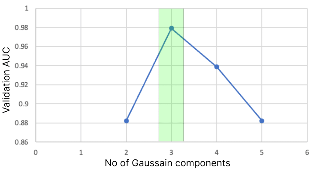
(a)

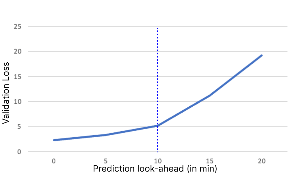
(b)

Figure 6. (a) Model performance vs number of Gaussian mixture components $C$ to predict by MDN; (b) Loss of the MDN (Eq. 3) vs Prediction look-ahead $\gamma$

7.2. Baseline Comparison (RQ2)

With our design choices fixed, that is, using a BiLSTM for encoding the metrics and then forecasting the distribution of the QoS metrics in a multi-task learning setting, we compare Outage-Watch with several baselines as described in §6. We use AUC-PR to compare the performance and tabulate the results in Table 4. Similar to the previous evaluations, we experiment with multiple values of $\gamma\in\{5,10,15,30\}$ min. The results demonstrate that our proposed approach of forecasting the distribution outperforms all other techniques, including traditional methods, by a significant margin. It has been shown to be a highly effective approach for predicting outages through QoS metrics

One key advantage of Outage-Watch is its ability to predict the probability of an outage occurring based on any threshold $\mathcal{T}$ (see Equation 5) since we are forecasting the distribution as opposed to just learning a classifier with the ground truth proxy labels. On the contrary, traditional methods are limited to predicting outages to a specific threshold (similar to the threshold used for creating the ground-truth labels in training data). As discussed in §5.1.3, we create proxy labels based on the threshold of 95%, i.e., if the metric value crosses the 95 percentile mark, it is considered to be a potential extreme event. Thus, the classifier network was trained using the generated proxy labels as a ground-truth. However, when we evaluate the distribution forecasted by Outage-Watch based on the probability of the metric value crossing a threshold of $\mathcal{T}=97\%$ and $\mathcal{T}=99\%$, we achieve high F1 scores, as seen in Table 5. $\gamma$ was maintained at 10 minutes. This flexibility in threshold selection is a major advantage of our proposed method and sets it apart from traditional techniques as the model need not be trained again to get the results on a different threshold.

Table 4. Performance of different models over different prediction windows in terms of AUC score.

Model	Prediction Look-Ahead ($\gamma$)
	5 mins	10 mins	15 mins	30 mins
Naive Bayes	0.593	0.592	0.592	0.582
Random Forest	0.873	0.868	0.867	0.824
Gradient Boost	0.870	0.854	0.828	0.822
BiLSTM+Classifier	0.909	0.914	0.930	0.927
Outage-Watch	0.981	0.982	0.977	0.975

Table 5. Performance of proposed model over different percentile thresholds in terms of F1 score.

Model	Prediction Thresholds ($\mathcal{T}$)
	95%	97%	99%
Outage-Watch	0.984	0.972	0.968

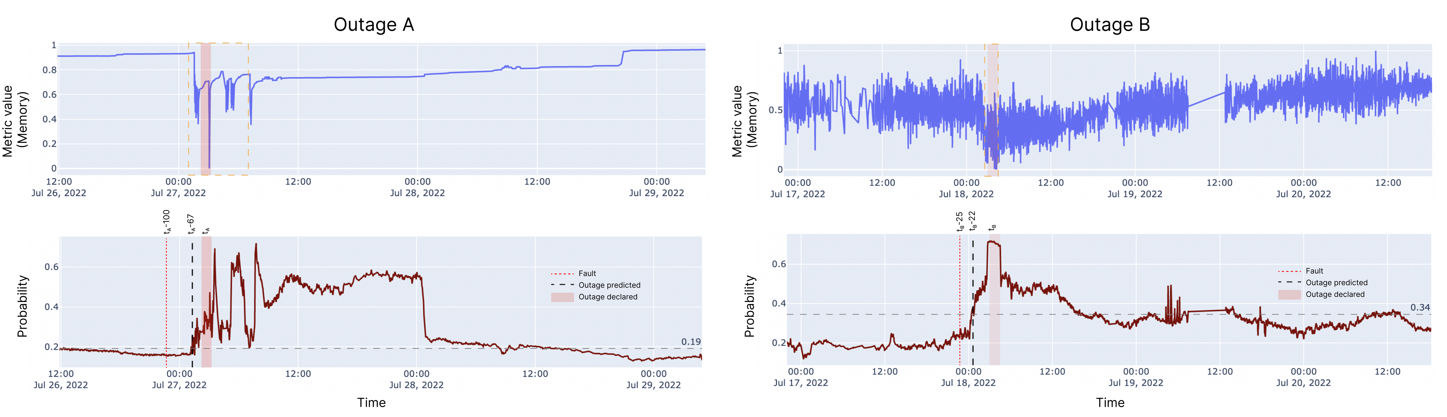
Figure 7. Analysis of the Outage-Watch’s performance on two real outages that happened during the deployment period. The upper plots are the metric values which shows deviations (actual value is masked), while the lower plots compute the probability of the metric value exceeding a threshold of $\mathcal{T}=99\%$. Outage-Watch was able to correctly predict both the outages in advance (in comparison to the current approach which is indicated by the light red rectangular shaded region).

7.3. Deployment Results (RQ3)

We deployed Outage-Watch in an enterprise system for 2 months and predicted the probability of impending outages. The overall objective of Outage-Watch is to predict outages in timely manner, thereby assisting the engineers. From the forecasted distribution, we first predict the probability of a metric value crossing the threshold $\mathcal{T}=99\%$. We then predict potential outage situations through the thresholding technique as described in §5.4.2 on the metric probability that crosses the threshold first. The threshold is generated based on the 9 weeks of training data. We report the precision and recall of the prediction made by Outage-Watch. We also report the reduction in time to detect outages by the model against the current reactive approach which is used to report an outage.

In this deployment, we implemented a continuous re-training strategy for Outage-Watch, updating the model after every outage detected with full data for up to two days after the outage ended. This approach was taken to ensure that the system state changes during an outage are reflected in the updated model. Our strategy balances effective model retraining with efficiency. It’s worth noting that our focus here does not encompass a robust retraining strategy (Wu et al., 2020) targeting drift issues. The potential for addressing data distribution changes, arising from factors such as the implementation of new business functionalities, could influence outage detection. However, this aspect falls outside the purview of our current work.

We present a case study for multiple outages that were flagged by the engineers during the deployment period and how Outage-Watch performed in forecasting them. During the deployment period, a total of 4 outages (Outage A, B, C, D) took place, out of which Outage A, B and C manifested through the QoS metrics in the cloud service. Outage-Watch was able to accurately predict all these three outages and reduced the mean time to detection as compared to the current approach followed by the engineers. However, Outage D was not evident through the QoS metrics and hence it was not predicted. We report the precision, recall and the reduction in MTTD for Outage A, B and C in Table 6. For each outage, we consider data from a day before and 2 days after to report the precision. Precision here refers to the number of outages correctly predicted over the number of times the probability value was above the threshold for a sustained period (15 mins). Recall refers to the number of outages predicted correctly over the total outages that could have been predicted, which is 3. Finally, MTTD reduction for each outage is reported as a percentage of (C - time of prediction)/(C-B) (see Figure 1 for the notations of B, C). We observe that Outage-Watch outperforms other baselines in terms of precision and recall. Recall is 100%, while precision is 30-40%. We also observe a large reduction in MTTD for Outage-Watch (‘-’ implies outage was not predicted). When EVL is used with Outage-Watch, precision improves.

Table 6. Results for outages predicted by different models using QoS metrics

Model	Precision	Recall	Reduction in MTTD
			Outage A	Outage B	Outage C
Naive Bayes	$1/14$	$1/3$	$24\%$	$-$	$-$
Random Forest	$1/11$	$1/3$	$0\%$	$-$	$-$
Gradient Boost	$2/12$	$2/3$	$0\%$	$76\%$	$-$
BiLSTM + Classifier	$2/10$	$2/3$	$-$	$56\%$	$26\%$
BiLSTM + MDN	$3/10$	3/3	$43\%$	$76\%$	$26\%$
Outage-Watch (BCE)	3/9	3/3	54%	$76\%$	27%
Outage-Watch (EVL)	3/8	3/3	$40\%$	80%	$26\%$

To provide a deeper understanding of how the system works, we present two case studies of outages (Outage A and Outage B) that were successfully predicted by Outage-Watch.

7.3.1. Outages Predicted

An illustration of these two outages and the performance of Outage-Watch are presented in Figure 7.

1. Outage A: The outage was auto-launched at time $t_{A}$ by the monitoring systems due to out-of-heap memory issues on several app store nodes in one of the regions. The system Outage-Watch was able to predict the out-of-heap memory issue correctly and flagged the outage $67$ minutes before the outage was actually launched. The system failed due to a fault in the event consumer queue which got stuck and was not processing since $t_{A}-100$ minutes in one of the regions.

2. Outage B: In another outage, alerts regarding high error rates in a service $\mathcal{S}$ were fired. The outage was auto-launched at $t_{B}$ by monitoring the high error rate. It was found that a faulty update in one of the AWS components had caused the component to fail. That component was being used by $\mathcal{S}$ and therefore after the update, $\mathcal{S}$ was unable to process incoming requests. The issue commenced since $t_{B}-25$ minutes. Outage-Watch correctly detected this outage and reduced the MTTD by 22 minutes from the auto-launched approach.

7.3.2. Outages Not Predicted

In addition, we also present a case study of an outage (Outage D) which occurred after a change was implemented that inadvertently tripped an UI feature blocking protocols from making requests. However, such outages due to UI issues are not meant to be manifested in the QoS metrics. As a result, it was not detected by our model. However, this is not a false negative in our case since no changes were observed on the QoS metrics, and hence Outage-Watch could not have detected the outage. This also highlights the limitations of our proposed method, as it relies on the monitoring metrics to predict outages.

7.4. Discussion

From the above results, we see that Outage-Watch performs better than the other comparable baselines, as well as on real-world deployment setting. However, it can be observed from Table 6 that Outage-Watch reports multiple false positives, which is dependent on the quality of threshold we choose to detect an outage. One can circumvent this issue by having a higher threshold (which might reduce the reduction in MTTD according to Figure 7). However, since we are working with the constraints of data, our training data set did not have any outages and the number of extreme events were very less as compared to the test data. This resulted in Youden’s index to compute a threshold lower than 0.5. However, with more data in the training set reflecting the extreme events, thresholding model becomes more proficient to distinguish true positives from the false positives, which results in a higher Youden’s index (Sokolova et al., 2006). As and when data arrives, Youden’s Index model should be retrained to get an improved threshold. Hence, thresholds can be re-adjusted as well with the predicted distribution, reducing the false positives.

However, in real-world scenarios, the presence of false positive cases is nuanced in this context. Our analysis of model predictions, along with SRE input, identified false positive cases where predicted extreme values didn’t lead to outages. Some of these issues were resolved manually or self-corrected. Consequently, the occurrences of false positives are not necessarily negative indicators, as they can capture mild issues that resemble potential disruptions. However, false positives are always undesirable in the workflow of SRE. While SREs can get insights from false positives, their presence is undesirable due to the risk of alert fatigue from frequent, possibly minor, predicted outputs. To tackle this, we provide the benefit of adaptable threshold selection as discussed in §5.4. A detailed study on how SREs can distinguish a false positive from a true positive output in their workflow remains an open question.

Overall, Outage-Watch proves to be very helpful for production outage management as it was able to predict the outages well in advance. This could help in reducing the severity and consequently helps with quick mitigation of the outages. We also highlight a limitation of the model, which relies solely on monitoring data and the QoS metrics and cannot predict those outages that are not indicative from these metrics. Nevertheless, we believe that by incorporating additional sources of data, such as log files and change details, we can improve the performance of our model in detecting these types of outages. Overall, our proposed method is a valuable tool for predicting outages using QoS metrics and has the potential to improve system performance and reliability.

8. Conclusion

In this paper, we present a novel approach Outage-Watch for predicting outages by forecasting the distribution of the relevant QoS metrics. This approach takes a time series input of multiple monitoring metrics representing the current system state within a time window to encode the information present in the time series in a vector representation. It then uses the encoded information to learn the distribution of the relevant metrics using a feed-forward neural network. In addition, Outage-Watch uses extreme value loss to classify the extreme events in a multi-task manner which helps in learning the distribution of the metrics in the tail.

At inference time, our model uses the distribution learnt to compute the probability of the metric to cross a certain threshold, and then predicts outages based on a thresholding technique. Our experiments on real-data show the efficacy of our method with an average AUC of 0.98. The applicability and robustness of our approach has been verified by deploying it on an enterprise system.

Future Works: Our future works include extending the evaluation duration on production systems to provide insights into long-term performance. Few interesting modifications include automated dynamic threshold selection and providing a confidence bound for our prediction to distinguish between the true positives and the false positive predictions. Furthermore, refining the definition of extreme events could enhance predictive capabilities. Incorporating diverse data sources, such as log files and trace data, may extend the scope of outage detection. We also plan on exploring robust re-training strategies (Wu et al., 2020) to improve model performance in production. Lastly, implementing a feedback loop or introducing human-in-the-loop dynamics may further refine the model’s predictive abilities.

9. Data Availability

The metrics data used in this research is proprietary and cannot be shared due to confidentiality agreements with the enterprise service provider. However, the model code along with a sample data are made available at Outage-Watch. The sample data includes the format of the input data required for the model with random metric values. Any real dataset can be pre-processed to the specified format for implementing the approach. We believe that the model code and sample data provided in the paper are sufficient for replication and working with similar datasets.

References

- (1)
- Ana (2016) 2016. Anatomy Of An IT Outage: Prediction and Detection. https://blog.opsramp.com/it-outage-prediction-and-detection. (2016).
- Met (2019) 2019. Metrics That Matter - ACM Queue. https://queue.acm.org/detail.cfm?id=3309571. (2019).
- Jus (2021) 2021. 7 Biggest Cloud Outages of the Past Year. https://techgenix.com/7-biggest-cloud-outages-services-2021/. (2021).
- clo (2022) 2022. Cloud Adoption Statistics for 2022. https://webtribunal.net/blog/cloud-adoption-statistics/. (2022).
- gra (2023) 2023. Grafana. https://grafana.com/. (2023).
- Met (2023) 2023. Metrics collected by the CloudWatch agent - Amazon CloudWatch. https://docs.aws.amazon.com/AmazonCloudWatch/latest/monitoring/metrics-collected-by-CloudWatch-agent.html. (2023).
- new (2023) 2023. New Relic. https://newrelic.com/. (2023).
- spl (2023) 2023. Splunk. https://www.splunk.com/. (2023).
- Abadi et al. (2016) Martín Abadi, Ashish Agarwal, Paul Barham, Eugene Brevdo, Zhifeng Chen, Craig Citro, Greg S Corrado, Andy Davis, Jeffrey Dean, Matthieu Devin, et al. 2016. Tensorflow: Large-scale machine learning on heterogeneous distributed systems. arXiv preprint arXiv:1603.04467 (2016).
- Adhikari and Agrawal (2013) Ratnadip Adhikari and R. K. Agrawal. 2013. An Introductory Study on Time Series Modeling and Forecasting. https://doi.org/10.48550/arXiv.1302.6613 arXiv:1302.6613 [cs.LG]
- Albeverio et al. (2006) Sergio Albeverio, Volker Jentsch, and Holger Kantz. 2006. Extreme events in nature and society. Springer Science & Business Media.
- Amazon (2023) Amazon. 2023. Post-Event Summaries. Retrieved from https://aws.amazon.com/cn/premiumsupport/technology/pes/.
- Anantharaman et al. (2018) Preethi Anantharaman, Mu Qiao, and Divyesh Jadav. 2018. Large scale predictive analytics for hard disk remaining useful life estimation. In 2018 IEEE International Congress on Big Data (BigData Congress). IEEE, 251–254. https://doi.org/10.1109/BigDataCongress.2018.00044
- Atlassian (2023) Atlassian. 2023. Atlassian incident management. Retrieved from https://www.atlassian.com/incident-management/incident-response/incident-commander.
- Azure (2023) Azure. 2023. Azure status history — Microsoft Azure. Retrieved from https://status.azure.com/en-us/status/history/.
- Beyer et al. (2016) Betsy Beyer, Chris Jones, Jennifer Petoff, and Niall Richard Murphy. 2016. Site Reliability Engineering: How Google Runs Production Systems (1st ed.). O’Reilly Media, Inc.
- Caruana (1997) Rich Caruana. 1997. Multitask learning. Machine learning 28, 1 (1997), 41–75.
- Chakraborty et al. (2023a) Sarthak Chakraborty, Shubham Agarwal, Shaddy Garg, Abhimanyu Sethia, Udit Narayan Pandey, Videh Aggarwal, and Shiv Saini. 2023a. ESRO: Experience Assisted Service Reliability against Outages. https://doi.org/10.48550/arXiv.2309.07230 arXiv:2309.07230 [cs.SE]
- Chakraborty et al. (2023b) Sarthak Chakraborty, Shaddy Garg, Shubham Agarwal, Ayush Chauhan, and Shiv Kumar Saini. 2023b. CausIL: Causal Graph for Instance Level Microservice Data. In Proceedings of the ACM Web Conference 2023 (Austin, TX, USA) (WWW ’23). Association for Computing Machinery, New York, NY, USA, 2905–2915. https://doi.org/10.1145/3543507.3583274
- Chatfield (2000) Chris Chatfield. 2000. Time-series forecasting. Chapman and Hall/CRC.
- Chen et al. (2016) Pengfei Chen, Yong Qi, and Di Hou. 2016. Causeinfer: automated end-to-end performance diagnosis with hierarchical causality graph in cloud environment. IEEE transactions on services computing 12, 2 (2016), 214–230. https://doi.org/10.1109/TSC.2016.2607739
- Chen et al. (2020b) Yujun Chen, Xian Yang, Hang Dong, Xiaoting He, Hongyu Zhang, Qingwei Lin, Junjie Chen, Pu Zhao, Yu Kang, Feng Gao, et al. 2020b. Identifying linked incidents in large-scale online service systems. In Proceedings of the 28th ACM joint meeting on European software engineering conference and symposium on the foundations of software engineering. 304–314. https://doi.org/10.1145/3368089.3409768
- Chen et al. (2019a) Yujun Chen, Xian Yang, Qingwei Lin, Hongyu Zhang, Feng Gao, Zhangwei Xu, Yingnong Dang, Dongmei Zhang, Hang Dong, Yong Xu, et al. 2019a. Outage prediction and diagnosis for cloud service systems. In The World Wide Web Conference. 2659–2665. https://doi.org/10.1145/3308558.3313501
- Chen et al. (2019b) Yujun Chen, Xian Yang, Qingwei Lin, Hongyu Zhang, Feng Gao, Zhangwei Xu, Yingnong Dang, Dongmei Zhang, Hang Dong, Yong Xu, et al. 2019b. Outage prediction and diagnosis for cloud service systems. In The World Wide Web Conference. 2659–2665. https://doi.org/10.1145/3308558.3313501
- Chen et al. (2020a) Zhuangbin Chen, Yu Kang, Liqun Li, Xu Zhang, Hongyu Zhang, Hui Xu, Yangfan Zhou, Li Yang, Jeffrey Sun, Zhangwei Xu, et al. 2020a. Towards intelligent incident management: why we need it and how we make it. In Proceedings of the 28th ACM Joint Meeting on European Software Engineering Conference and Symposium on the Foundations of Software Engineering. 1487–1497. https://doi.org/10.1145/3368089.3417055
- Chen et al. (2022) Zhuangbin Chen, Jinyang Liu, Yuxin Su, Hongyu Zhang, Xiao Ling, Yongqiang Yang, and Michael R Lyu. 2022. Adaptive performance anomaly detection for online service systems via pattern sketching. In Proceedings of the 44th International Conference on Software Engineering. 61–72. https://doi.org/10.1145/3510003.3510085
- Cho et al. (2014) Kyunghyun Cho, Bart Van Merriënboer, Caglar Gulcehre, Dzmitry Bahdanau, Fethi Bougares, Holger Schwenk, and Yoshua Bengio. 2014. Learning phrase representations using RNN encoder-decoder for statistical machine translation. arXiv preprint arXiv:1406.1078 (2014). https://doi.org/10.3115/v1/D14-1179
- Coles et al. (2001) Stuart Coles, Joanna Bawa, Lesley Trenner, and Pat Dorazio. 2001. An introduction to statistical modeling of extreme values. Vol. 208. Springer.
- crn (2023) crn. 2023. 15-biggest-cloud-outages. Retrieved from https://www.crn.com/news/cloud/the-15-biggest-cloud-outages-of-2022.
- Cui et al. (2018) Zhiyong Cui, Ruimin Ke, Ziyuan Pu, and Yinhai Wang. 2018. Deep bidirectional and unidirectional LSTM recurrent neural network for network-wide traffic speed prediction. arXiv preprint arXiv:1801.02143 (2018). https://doi.org/10.48550/arXiv.2005.11627
- Dang et al. (2019) Yingnong Dang, Qingwei Lin, and Peng Huang. 2019. Aiops: real-world challenges and research innovations. In 2019 IEEE/ACM 41st International Conference on Software Engineering: Companion Proceedings (ICSE-Companion). IEEE, 4–5. https://doi.org/10.1109/ICSE-Companion.2019.00023
- Dasgupta and Osogami (2017) Sakyasingha Dasgupta and Takayuki Osogami. 2017. Nonlinear dynamic Boltzmann machines for time-series prediction. In Proceedings of the AAAI conference on artificial intelligence, Vol. 31. https://doi.org/10.1609/aaai.v31i1.10806
- Ding et al. (2019) Daizong Ding, Mi Zhang, Xudong Pan, Min Yang, and Xiangnan He. 2019. Modeling extreme events in time series prediction. In Proceedings of the 25th ACM SIGKDD International Conference on Knowledge Discovery & Data Mining. 1114–1122. https://doi.org/10.1145/3292500.3330896
- dos Santos Lima et al. (2017) Fernando Dione dos Santos Lima, Gabriel Maia Rocha Amaral, Lucas Goncalves de Moura Leite, João Paulo Pordeus Gomes, and Javam de Castro Machado. 2017. Predicting failures in hard drives with LSTM networks. In 2017 Brazilian Conference on Intelligent Systems (BRACIS). IEEE, 222–227. https://doi.org/10.1109/BRACIS.2017.72
- Friederichs and Thorarinsdottir (2012) Petra Friederichs and Thordis L Thorarinsdottir. 2012. Forecast verification for extreme value distributions with an application to probabilistic peak wind prediction. Environmetrics 23, 7 (2012), 579–594.
- Ghil et al. (2011) M Ghil, P Yiou, Stéphane Hallegatte, BD Malamud, P Naveau, A Soloviev, P Friederichs, V Keilis-Borok, D Kondrashov, V Kossobokov, et al. 2011. Extreme events: dynamics, statistics and prediction. Nonlinear Processes in Geophysics 18, 3 (2011), 295–350.
- Glorot et al. (2011) Xavier Glorot, Antoine Bordes, and Yoshua Bengio. 2011. Deep sparse rectifier neural networks. In Proceedings of the fourteenth international conference on artificial intelligence and statistics. JMLR Workshop and Conference Proceedings, 315–323.
- Google (2023a) Google. 2023a. Google Cloud Service Health. Retrieved from https://status.cloud.google.com/summary.
- Google (2023b) Google. 2023b. Google SRE book. Retrieved from https://landing.google.com/sre/sre-book/chapters/managing-incidents/.
- Graves and Schmidhuber (2005) Alex Graves and Jürgen Schmidhuber. 2005. Framewise phoneme classification with bidirectional LSTM and other neural network architectures. Neural networks 18, 5-6 (2005), 602–610. https://doi.org/10.1016/j.neunet.2005.06.042
- Gurland (1954) John Gurland. 1954. Hypothesis Testing in Time Series Analysis.
- Haan and Ferreira (2006) Laurens Haan and Ana Ferreira. 2006. Extreme value theory: an introduction. Vol. 3. Springer.
- Hochreiter and Schmidhuber (1997) Sepp Hochreiter and Jürgen Schmidhuber. 1997. Long short-term memory. Neural computation 9, 8 (1997), 1735–1780. https://doi.org/10.1162/neco.1997.9.8.1735
- Hyndman and Khandakar (2008) Rob J Hyndman and Yeasmin Khandakar. 2008. Automatic time series forecasting: the forecast package for R. Journal of statistical software 27 (2008), 1–22.
- Ikram et al. (2022) Muhammad Azam Ikram, Sarthak Chakraborty, Subrata Mitra, Shiv Saini, Saurabh Bagchi, and Murat Kocaoglu. 2022. Root Cause Analysis of Failures in Microservices through Causal Discovery. In Advances in Neural Information Processing Systems, Alice H. Oh, Alekh Agarwal, Danielle Belgrave, and Kyunghyun Cho (Eds.). https://openreview.net/forum?id=weoLjoYFvXY
- informationweek (2023a) informationweek. 2023a. cloud is fragile. Retrieved from https://www.informationweek.com/cloud/special-report-how-fragile-is-the-cloud-really-.
- informationweek (2023b) informationweek. 2023b. cloud outages. Retrieved from https://www.informationweek.com/cloud/cloud-outages-causes-consequences-prevention-recovery.
- Jiang et al. (2009) Guofei Jiang, Haifeng Chen, Kenji Yoshihira, and Akhilesh Saxena. 2009. Ranking the importance of alerts for problem determination in large computer systems. In Proceedings of the 6th international conference on autonomic computing. 3–12. https://doi.org/10.1145/1555228.1555232
- Laptev et al. (2017) Nikolay Laptev, Jason Yosinski, Li Erran Li, and Slawek Smyl. 2017. Time-series extreme event forecasting with neural networks at uber. In International conference on machine learning, Vol. 34. 1–5.
- Li et al. (2021) Liqun Li, Xu Zhang, Xin Zhao, Hongyu Zhang, Yu Kang, Pu Zhao, Bo Qiao, Shilin He, Pochian Lee, Jeffrey Sun, et al. 2021. Fighting the Fog of War: Automated Incident Detection for Cloud Systems. In 2021 USENIX Annual Technical Conference (USENIX ATC 21). 131–146.
- Li et al. (2022) Mingjie Li, Zeyan Li, Kanglin Yin, Xiaohui Nie, Wenchi Zhang, Kaixin Sui, and Dan Pei. 2022. Causal Inference-Based Root Cause Analysis for Online Service Systems with Intervention Recognition. In Proceedings of the 28th ACM SIGKDD Conference on Knowledge Discovery and Data Mining. 3230–3240. https://doi.org/10.1145/3534678.3539041
- Lim and Zohren (2021) Bryan Lim and Stefan Zohren. 2021. Time-series forecasting with deep learning: a survey. Philosophical Transactions of the Royal Society A 379, 2194 (2021), 20200209.
- Lin et al. (2014) Derek Lin, Rashmi Raghu, Vivek Ramamurthy, Jin Yu, Regunathan Radhakrishnan, and Joseph Fernandez. 2014. Unveiling clusters of events for alert and incident management in large-scale enterprise it. In Proceedings of the 20th ACM SIGKDD international conference on Knowledge discovery and data mining. 1630–1639. https://doi.org/10.1145/2623330.2623360
- Lin et al. (2017b) Tao Lin, Tian Guo, and Karl Aberer. 2017b. Hybrid neural networks for learning the trend in time series. In Proceedings of the twenty-sixth international joint conference on artificial intelligence. 2273–2279.
- Lin et al. (1996) Tsungnan Lin, Bill G Horne, Peter Tino, and C Lee Giles. 1996. Learning long-term dependencies in NARX recurrent neural networks. IEEE Transactions on Neural Networks 7, 6 (1996), 1329–1338. https://doi.org/10.1109/72.548162
- Lin et al. (2017a) Tsung-Yi Lin, Priya Goyal, Ross Girshick, Kaiming He, and Piotr Dollár. 2017a. Focal loss for dense object detection. In Proceedings of the IEEE international conference on computer vision. 2980–2988. https://doi.org/10.1109/TPAMI.2018.2858826
- Lou et al. (2013) Jian-Guang Lou, Qingwei Lin, Rui Ding, Qiang Fu, Dongmei Zhang, and Tao Xie. 2013. Software analytics for incident management of online services: An experience report. In 2013 28th IEEE/ACM International Conference on Automated Software Engineering (ASE). IEEE, 475–485. https://doi.org/10.1109/ASE.2013.6693105
- Lu et al. (2020) Sidi Lu, Bing Luo, Tirthak Patel, Yongtao Yao, Devesh Tiwari, and Weisong Shi. 2020. Making disk failure predictions smarter!. In FAST. 151–167.
- Oki et al. (2018) Motoyuki Oki, Koh Takeuchi, and Yukio Uematsu. 2018. Mobile network failure event detection and forecasting with multiple user activity data sets. In Proceedings of the AAAI Conference on Artificial Intelligence, Vol. 32. https://doi.org/10.1609/aaai.v32i1.11422
- Park et al. (2018) Daehyung Park, Yuuna Hoshi, and Charles C Kemp. 2018. A multimodal anomaly detector for robot-assisted feeding using an lstm-based variational autoencoder. IEEE Robotics and Automation Letters 3, 3 (2018), 1544–1551. https://doi.org/10.1109/LRA.2018.2801475
- Park et al. (2019) Pangun Park, Piergiuseppe Di Marco, Hyejeon Shin, and Junseong Bang. 2019. Fault detection and diagnosis using combined autoencoder and long short-term memory network. Sensors 19, 21 (2019), 4612. https://doi.org/10.3390/s19214612
- Pudjihartono et al. (2022) Nicholas Pudjihartono, Tayaza Fadason, Andreas W Kempa-Liehr, and Justin M O’Sullivan. 2022. A review of feature selection methods for machine learning-based disease risk prediction. Frontiers in Bioinformatics 2 (2022), 927312. https://doi.org/10.3389/fbinf.2022.927312
- Qin et al. (2017) Yao Qin, Dongjin Song, Haifeng Chen, Wei Cheng, Guofei Jiang, and Garrison Cottrell. 2017. A dual-stage attention-based recurrent neural network for time series prediction. arXiv preprint arXiv:1704.02971 (2017).
- readitquik (2023) readitquik. 2023. ReadItQuick Cloud Failures. Retrieved from https://www.readitquik.com/articles/cloud-3/6-cloud-computing-failures-that-shocked-the-world/.
- Reynolds (2009) Douglas Reynolds. 2009. Gaussian Mixture Models. Springer US, Boston, MA, 659–663. https://doi.org/10.1007/978-0-387-73003-5_196
- Ruder (2017) Sebastian Ruder. 2017. An Overview of Multi-Task Learning in Deep Neural Networks. arXiv:1706.05098 [cs.LG]
- Schölkopf and Smola (2002) Bernhard Schölkopf and Alexander J Smola. 2002. Learning with kernels: support vector machines, regularization, optimization, and beyond. MIT press. https://doi.org/10.7551/mitpress/4175.001.0001
- Schuster and Paliwal (1997) M. Schuster and K.K. Paliwal. 1997. Bidirectional recurrent neural networks. IEEE Transactions on Signal Processing 45, 11 (1997), 2673–2681. https://doi.org/10.1109/78.650093
- Shao et al. (2020) Wei Shao, Siyu Tan, Sichen Zhao, Kyle Kai Qin, Xinhong Hei, Jeffrey Chan, and Flora D Salim. 2020. Incorporating lstm auto-encoders in optimizations to solve parking officer patrolling problem. ACM Transactions on Spatial Algorithms and Systems (TSAS) 6, 3 (2020), 1–21. https://doi.org/10.1145/3380966
- Siami Namini et al. (2018) Sima Siami Namini, Neda Tavakoli, and Akbar Siami Namin. 2018. A Comparison of ARIMA and LSTM in Forecasting Time Series. 1394–1401. https://doi.org/10.1109/ICMLA.2018.00227
- Sofaer et al. (2019) Helen R Sofaer, Jennifer A Hoeting, and Catherine S Jarnevich. 2019. The area under the precision-recall curve as a performance metric for rare binary events. Methods in Ecology and Evolution 10, 4 (2019), 565–577.
- Sokolova et al. (2006) Marina Sokolova, Nathalie Japkowicz, and Stan Szpakowicz. 2006. Beyond Accuracy, F-Score and ROC: A Family of Discriminant Measures for Performance Evaluation. In AI 2006: Advances in Artificial Intelligence, Abdul Sattar and Byeong-ho Kang (Eds.). Springer Berlin Heidelberg, Berlin, Heidelberg, 1015–1021. https://doi.org/10.1007/11941439_114
- Su et al. (2019) Ya Su, Youjian Zhao, Chenhao Niu, Rong Liu, Wei Sun, and Dan Pei. 2019. Robust anomaly detection for multivariate time series through stochastic recurrent neural network. In Proceedings of the 25th ACM SIGKDD international conference on knowledge discovery & data mining. 2828–2837.
- Torres et al. (2021) José F Torres, Dalil Hadjout, Abderrazak Sebaa, Francisco Martínez-Álvarez, and Alicia Troncoso. 2021. Deep learning for time series forecasting: a survey. Big Data 9, 1 (2021), 3–21.
- Tuli et al. (2022) Shreshth Tuli, Giuliano Casale, and Nicholas R Jennings. 2022. TranAD: deep transformer networks for anomaly detection in multivariate time series data. Proceedings of the VLDB Endowment 15, 6 (2022), 1201–1214. https://doi.org/10.14778/3514061.3514067
- Wu et al. (2020) Yinjun Wu, Edgar Dobriban, and Susan Davidson. 2020. Deltagrad: Rapid retraining of machine learning models. In International Conference on Machine Learning. PMLR, 10355–10366. https://doi.org/PMLR119:10355-10366
- Xu et al. (2018) Yong Xu, Kaixin Sui, Randolph Yao, Hongyu Zhang, Qingwei Lin, Yingnong Dang, Peng Li, Keceng Jiang, Wenchi Zhang, Jian-Guang Lou, et al. 2018. Improving service availability of cloud systems by predicting disk error. In 2018 USENIX Annual Technical Conference (USENIXATC 18). 481–494.
- Yang et al. (2015) Jianbo Yang, Minh Nhut Nguyen, Phyo Phyo San, Xiao Li Li, and Shonali Krishnaswamy. 2015. Deep convolutional neural networks on multichannel time series for human activity recognition. In Twenty-fourth international joint conference on artificial intelligence.
- Youden (1950) William J Youden. 1950. Index for rating diagnostic tests. Cancer 3, 1 (1950), 32–35.
- Zhang et al. (2018) Shenglin Zhang, Ying Liu, Weibin Meng, Zhiling Luo, Jiahao Bu, Sen Yang, Peixian Liang, Dan Pei, Jun Xu, Yuzhi Zhang, et al. 2018. Prefix: Switch failure prediction in datacenter networks. Proceedings of the ACM on Measurement and Analysis of Computing Systems 2, 1 (2018), 1–29. https://doi.org/10.1145/3179405
- Zhang et al. (2019) Xu Zhang, Junghyun Kim, Qingwei Lin, Keunhak Lim, Shobhit O Kanaujia, Yong Xu, Kyle Jamieson, Aws Albarghouthi, Si Qin, Michael J Freedman, et al. 2019. Cross-dataset time series anomaly detection for cloud systems. In 2019 USENIX Annual Technical Conference (USENIX ATC 19). 1063–1076.
- Zhao et al. (2020a) Nengwen Zhao, Junjie Chen, Xiao Peng, Honglin Wang, Xinya Wu, Yuanzong Zhang, Zikai Chen, Xiangzhong Zheng, Xiaohui Nie, Gang Wang, et al. 2020a. Understanding and handling alert storm for online service systems. In Proceedings of the ACM/IEEE 42nd International Conference on Software Engineering: Software Engineering in Practice. 162–171. https://doi.org/10.1145/3377813.3381363
- Zhao et al. (2020b) Nengwen Zhao, Junjie Chen, Zhou Wang, Xiao Peng, Gang Wang, Yong Wu, Fang Zhou, Zhen Feng, Xiaohui Nie, Wenchi Zhang, Kaixin Sui, and Dan Pei. 2020b. Real-Time Incident Prediction for Online Service Systems. Association for Computing Machinery, New York, NY, USA, 315–326. https://doi.org/10.1145/3368089.3409672
- Zhao et al. (2020c) Nengwen Zhao, Panshi Jin, Lixin Wang, Xiaoqin Yang, Rong Liu, Wenchi Zhang, Kaixin Sui, and Dan Pei. 2020c. Automatically and adaptively identifying severe alerts for online service systems. In IEEE INFOCOM 2020-IEEE Conference on Computer Communications. IEEE, 2420–2429. https://doi.org/10.1109/INFOCOM41043.2020.9155219
- Zhu et al. (2017) Yu Zhu, Hao Li, Yikang Liao, Beidou Wang, Ziyu Guan, Haifeng Liu, and Deng Cai. 2017. What to Do Next: Modeling User Behaviors by Time-LSTM.. In IJCAI, Vol. 17. 3602–3608.