Reference Vertical Excitation Energies for Transition Metal Compounds

Abstract

To enrich and enhance the diversity of the quest database of highly-accurate excitation energies [Véril et al., WIREs Comput. Mol. Sci. 11, e1517 (2021)], we report vertical transition energies in transition metal compounds. Eleven diatomic molecules with singlet or doublet ground state containing a fourth-row transition metal (CuCl, CuF, CuH, ScF, ScH, ScO, ScS, TiN, ZnH, ZnO, and ZnS) are considered and the corresponding excitation energies are computed using high-level coupled-cluster (CC) methods, namely CC3, CCSDT, CC4, and CCSDTQ, as well as multiconfigurational methods such as CASPT2 and NEVPT2. In some cases, to provide more comprehensive benchmark data, we also provide full configuration interaction estimates computed with the “Configuration Interaction using a Perturbative Selection made Iteratively” (CIPSI) method. Based on these calculations, theoretical best estimates of the transition energies are established in both the aug-cc-pVDZ and aug-cc-pVTZ basis sets. This allows us to accurately assess the performance of CC and multiconfigurational methods for this specific set of challenging transitions. Furthermore, comparisons with experimental data and previous theoretical results are also reported.

I Introduction

Understanding the electronic structure of transition metal compounds Khomskii (2014) is critical for unraveling their specific behaviors and applications in a wide range of fields, such as chemistry and biology. Trautwein (1997) Their electronic structure is characterized by the presence of partially filled $d$ orbitals in the transition metal atoms, which gives rise to their unique properties such as variable oxidation states, Askerka, Brudvig, and Batista (2016) magnetic behavior, Ebert (1996); van Oudenaarden et al. (1998); Gerhard et al. (2010) and catalytic activity. Melius (1976) The empty $d$ orbitals can participate in chemical reactions, Bolm, Palazzi, and Beckmann allowing for the transfer of electrons during redox processes. Ma et al. (2021) Transition metal catalysts find applications in various industrial processes, including hydrogenation, oxidation, and carbon-carbon bond formation. García-Melchor et al. (2013); Guest et al. (2015); Sperger et al. (2015)

From a general perspective, investigating molecular excited states is essential for understanding their reactivity, photophysical properties, and catalytic behavior. Indeed, the presence of the excited electron modifies the electronic structure of the molecule, affecting reactions such as bond activation, insertion, or reductive processes. Bernardi et al. (1990); Klessinger and Michl (1995); Robb et al. (2007); Delgado et al. (2010); Olivucci (2010) The excited states of molecules containing transition metals have very peculiar characteristics and reactivity due to the presence of the transition metal atom. For example, in photocatalysis, the absorption of light can lead to the formation of reactive excited states that participate in photochemical reactions. Twilton et al. (2017)

Experimentally characterizing excited states in transition metal compounds is challenging due to their often short lifetimes and low transition probabilities. Transient absorption spectroscopy, Geneaux et al. (2019) time-resolved techniques, Haglund (2007) and advanced spectroscopic methods are required to observe and analyze the excited-state behavior. Additionally, the identification and assignment of the observed spectral features are challenging due to the complexity of the excited-state manifold in these systems. Bokarev and Kühn (2019)

From a theoretical point of view, the study of excited states in transition metal compounds presents several challenges due to their complex electronic structures and intricate interactions. Harrison (2000); Harvey (2006); Zhao and Truhlar (2006); Sperger, Sanhueza, and Schoenebeck (2016); Santoro et al. (2016); Friesner and Jerome (2017); Bokarev and Kühn (2019); Hait et al. (2019) First, they often require sophisticated theoretical methods to accurately describe the electronic structure of both their ground state and their excited states. Roos et al. (1996a); Piecuch et al. (2002); Dreuw and Head-Gordon (2005); Krylov (2006); Sneskov and Christiansen (2012); González, Escudero, and Serrano-Andrès (2012); Laurent and Jacquemin (2013); Adamo and Jacquemin (2013); Ghosh et al. (2018); Blase et al. (2020); Loos et al. (2020a) These calculations are computationally demanding and require the use of high-level quantum chemical approaches, Helgaker, Jørgensen, and Olsen (2013) such as multireference methods, Khedkar and Roemelt (2021) to account for the strong correlation effects present in many transition metal systems (see below). Buendía et al. (2013); Aoto et al. (2017); Shee et al. (2019); Wagner and Mitáš (2003, 2007); Diedrich, Lüchow, and Grimme (2005); Caffarel et al. (2005, 2014); Doblhoff-Dier et al. (2016); Scemama et al. (2018); Giner et al. (2018); Suo et al. (2017); Nooijen and Lotrich (2000); Körbel et al. (2014) Second, the large number of electrons and basis functions involved in these calculations further add to the computational complexity. Third, transition metal compounds often exhibit multiple spin states, which affects not only their reactivity but also their magnetic properties. Wang, Avendaño, and Dunbar (2011) This leads to the accumulation of excited states with potentially the same spin and spatial symmetries in a very narrow energy window, which complicates the interpretation of experimental results and theoretical calculations. Loos et al. (2020a); Véril et al.

As mentioned above, transition metal derivatives often exhibit strong (or static) correlation, which refers to the intricate interactions among electrons occupying the $d$ orbitals. Strong correlation is often a signature of the multiconfigurational character of the electronic wave function, meaning that the ground state and/or excited states cannot be accurately described by a single Slater determinant (single-reference wave function) but require a linear combination of multiple determinants (multireference wave function) to accurately capture the electronic structure. The remaining dynamic correlation must also be taken into account as it systematically plays a crucial role in describing the excited states.

To accurately describe the multiconfigurational character and strong electron correlation, methods based on configuration interaction (CI) are commonly employed. Szabo and Ostlund (1989) This class of methods allows for the mixing of different electronic configurations and provides a flexible framework to capture the electronic correlation effects. If one considers all possible electronic configurations, the resulting full CI (FCI) wave function corresponds to the exact solution of the Schrödinger equation within a given one-electron basis set. Unfortunately, the ensemble of these configurations, known as the Hilbert space, has a size that grows exponentially fast with the system size, leading to a prohibitive computational cost in most applications.

Multiconfigurational self-consistent field methods, such as complete-active-space self-consistent field (CASSCF), account for all determinants generated by distributing a given number of electrons in a given number of active orbitals, therefore incorporating, by design, static correlation. Besides, unlike in CI, orbitals are variationally optimized. The missing dynamic correlation is usually recovered via low-order perturbation theory as in the complete-active-space second-order perturbation theory (CASPT2) Andersson et al. (1990); Andersson, Malmqvist, and Roos (1992); Roos et al. (1995) or the $N$-electron valence state second-order perturbation theory (NEVPT2). Angeli, Cimiraglia, and Malrieu (2001); Angeli et al. (2001); Angeli, Cimiraglia, and Malrieu (2002); Angeli et al. (2006) For CASSCF-based methods, selecting an appropriate active space is critical for capturing the important electron correlation effects while keeping the computational cost manageable. In transition metal compounds, the active space typically involves the $d$ orbitals of the metal center and the orbitals involved in the ligand interactions. Choosing an appropriate active space is a delicate balance between including a sufficient number of active orbitals to describe the correlation effects and keeping a reasonable computational cost.

Coupled-cluster (CC) methods offer an alternative approach, based on an exponential ansatz of the wave function, that allows for size-extensive and systematically improvable calculations towards the FCI limit. These methods exhibit polynomial scaling and have been extensively studied in the literature. Čížek (1966, 1969); Paldus (1992); Crawford and Schaefer (2000); Bartlett and Musiał (2007); Shavitt and Bartlett (2009) Coupled-cluster methods systematically incorporate higher levels of excitations to improve accuracy. For instance, CC with singles and doubles (CCSD), Purvis III and Bartlett (1982); Scuseria et al. (1987); Koch et al. (1990); Stanton and Bartlett (1993); Stanton (1993) CC with singles, doubles, and triples (CCSDT), Noga and Bartlett (1987); Scuseria and Schaefer (1988); Watts and Bartlett (1994); Kucharski et al. (2001) and CC with singles, doubles, triples, and quadruples (CCSDTQ) Kucharski and Bartlett (1991); Kállay and Surján (2001); Hirata (2004); Kállay, Gauss, and Szalay (2003); Kállay and Gauss (2004) can be obtained by successively adding higher excitation levels. The computational cost of these methods scales as $\order*{N^{6}}$, $\order*{N^{8}}$, and $\order*{N^{10}}$, respectively. Moreover, to reduce computational expenses, each of these methods can be approximated by the CC$n$ family of methods. This family includes CC2 ($\order*{N^{5}}$), Christiansen, Koch, and Jørgensen (1995a); Hättig and Weigend (2000) CC3 ($\order*{N^{7}}$), Christiansen, Koch, and Jørgensen (1995b); Koch et al. (1995, 1997); Hald et al. (2001); Paul, Myhre, and Koch (2021) and CC4 ($\order*{N^{9}}$). Kállay and Gauss (2004, 2005); Matthews and Stanton (2015); Loos et al. (2021a); Loos and Romaniello (2022) These variants provide cost-effective alternatives while still maintaining acceptable levels of accuracy compared to their “complete” variant. Excited-state energies and properties can be obtained within the CI framework by searching for higher roots of the CI matrix and their corresponding eigenvectors. Similarly, at CC level, one can access excited states using the equation-of-motion (EOM) Rowe (1968); Emrich (1981); Sekino and Bartlett (1984); Geertsen, Rittby, and Bartlett (1989); Stanton and Bartlett (1993); Comeau and Bartlett (1993); Watts and Bartlett (1994) or linear-response (LR) Monkhorst (1977); Dalgaard and Monkhorst (1983); Sekino and Bartlett (1984); Koch and Jørgensen (1990); Koch et al. (1990) formalisms.

II The quest database

Benchmark sets and their corresponding reference data serve as a cornerstone in electronic structure theory, supporting the development, validation, and improvement of computational methods for both the ground state Pople et al. (1989); Curtiss et al. (1991, 1997, 1998); Curtiss, Redfern, and Raghavachari (2007); Jurečka et al. (2006); Řezáč, Riley, and Hobza (2011); van Setten et al. (2015); Stuke et al. (2020); Tajti et al. (2004); Bomble et al. (2006); Harding et al. (2008); Motta et al. (2017); Williams et al. (2020); Zhao and Truhlar (2006); Mardirossian and Head-Gordon (2017); Goerigk and Grimme (2010a, 2011a, 2011b); Goerigk et al. (2017) and the excited states. Schreiber et al. (2008); Silva-Junior et al. (2008, 2010a, 2010b, 2010c); Leang, Zahariev, and Gordon (2012); Schwabe and Goerigk ; Casanova-Paez, Dardis, and Goerigk (2019); Casanova-Paez and Goerigk (2020); Furche and Ahlrichs (2002); Send, Kühn, and Furche (2011); Winter et al. (2013); Dierksen and Grimme (2004); Goerigk and Grimme (2010b); Jacquemin et al. (2012); Jacquemin, Duchemin, and Blase (2015); Kozma et al. (2020) In the context of molecular excited states, a benchmark set refers to a collection of molecules with known reference data that is used to evaluate the accuracy, reliability, and limitations of computational methods in predicting the properties of electronic excited states, such as excitation energies, oscillator strengths, transition dipole moments, and other spectroscopic observables.

They provide a standardized framework for evaluating the performance of different computational methods in predicting excited-state properties, contributing to the reproducibility and transparency of computational studies in the field. By comparing different methods against each other, researchers can identify the strengths and weaknesses of different approaches and gain insights into their limitations, hence guiding the development of new computational methods for electronic excited states. Besides, these investigations also assist researchers and practitioners in selecting appropriate methods for specific applications or molecules.

The reference data are typically obtained from highly-accurate theoretical calculations or experimental measurements. Their accuracy and reliability are mandatory for ensuring the meaningfulness of the benchmarking process. In some cases, reference data may be obtained from experiments, such as spectroscopic measurements or photochemical data, but these experimental values are not always available or may have uncertainties. Loos and Jacquemin (2019a) The selection of molecules for a benchmark set aims to cover a diverse range of electronic structures and properties, including different types of excited states, as well as a variety of chemical environments and molecular sizes. Importantly, it should also include challenging cases that test the capabilities of the methods under investigation.

Since 2018, our research groups have made significant efforts to develop a comprehensive and diverse database of highly-accurate vertical excitation energies for small- and medium-sized (organic) molecules. This database, named quest, Loos, Scemama, and Jacquemin (2020); Véril et al. has been meticulously curated and expanded over time. It currently comprises seven subsets, as illustrated in Fig. 1:

• quest#1: This subset consists of 110 vertical excitation energies (and oscillator strengths) in small molecules containing 1 to 3 non-hydrogen atoms. Loos et al. (2018) Primarily focused on singly-excited states, the theoretical best estimates (TBEs) were determined using FCI calculations.

• quest#2: Comprising 20 vertical transition energies for doubly-excited states in 14 small and medium-sized molecules, Loos et al. (2019) this subset relied predominantly on FCI calculations to define the TBEs, except for the largest molecules in the set.

• quest#3: This subset encompasses 238 excitation energies (and oscillator strengths) for 27 medium-sized molecules containing 4 to 6 non-hydrogen atoms. Loos et al. (2020b) The TBEs in this subset were originally defined using CCSDT or CCSDTQ methods, and more recent improvements have been made with CC4 and CCSDTQ approaches. Loos et al. (2021b, 2022)

• quest#4: Composed of two distinct parts, this subset includes an “exotic” subset of 30 vertical excitation energies for closed-shell molecules containing F, Cl, P, and Si atoms, and a “radical” subset of 51 doublet-doublet transitions in 24 small open-shell molecules. Loos et al. (2020c) In total, there are 81 TBEs, mostly obtained with FCI.

• quest#5: Featuring 80 excitation energies in 13 (mostly large) molecules, this subset mostly contains TBE calculations at the CCSDT level. Véril et al.

• quest#6: Specifically designed for the study of intramolecular charge-transfer transitions, this subset provides highly-accurate vertical excitation energies for 30 such transitions in 17 $\pi$-conjugated compounds obtained at the CCSDT level. Loos et al. (2021a)

• quest#7: This subset contains 91 vertical excitation energies for 10 bicyclic molecules computed at the CC3 or CCSDT levels. Loos and Jacquemin (2021)

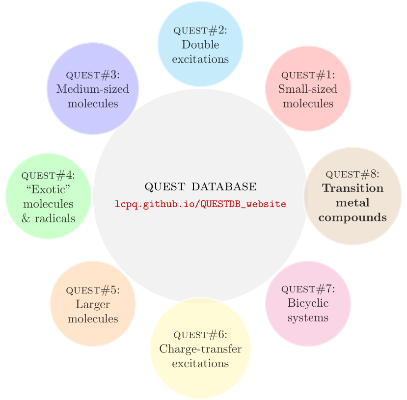
Figure 1: The 8 subsets composing the quest database of highly-accurate excitation energies with the inclusion of a new subset gathering excited states of transition metal compounds (quest#8).

As evidenced by the above description, quest employs FCI and high-order CC methods to generate highly-accurate reference data in triple-$\zeta$ basis, alongside additional basis set corrections when possible. In most cases, geometry optimization has been carried out at the CC3/aug-cc-pVTZ level. A significant advantage of the quest dataset is its independence from experimental values, eliminating potential biases associated with experiments and facilitating direct theoretical comparisons. The employed protocol ensures uniformity, enabling straightforward cross-comparisons. This approach allowed the benchmarking of a wide range of excited-state wave function methods, including those accounting for double and triple excitations, as well as multiconfigurational methods. Furthermore, chemically-accurate theoretical 0-0 energies have been computed, providing a more direct comparison to experimental data. Loos, Galland, and Jacquemin (2018); Loos and Jacquemin (2019b, a) Presently, our ongoing efforts are dedicated to obtaining highly-accurate excited-state properties such as dipoles and oscillator strengths for small and medium-sized molecules. Chrayteh et al. (2021); Sarkar et al. (2021, 2022); Damour et al. (2022)

The creation of the quest dataset involved a very significant computational effort, with numerous calculations performed for each of the associated articles. Loos et al. (2018, 2019, 2020b, 2020c); Véril et al. ; Loos et al. (2021a); Loos and Jacquemin (2021) To access and manipulate the data, a web application has been developed and hosted on a GitHub repository (https://github.com/LCPQ/QUESTDB_website). The web application can be accessed at https://lcpq.github.io/QUESTDB_website, providing users with the ability to plot statistical indicators for selected subsets of molecules, methods, and basis sets.

The utilization of the quest database as a benchmark for excited-state methods has gained attraction among research groups worldwide. For instance, the database has been employed to assess orbital-optimized DFT for double excitations, Hait and Head-Gordon (2020, 2021) multistate DFT, Zhu et al. (2023) and TD-DFT. Liang et al. (2022) Additionally, it has facilitated the evaluation of hybrid Grotjahn and Kaupp (2021) and double hybrid Casanova-Páez, Dardis, and Goerigk (2019); Casanova-Páez and Goerigk (2021); Mester and Kállay (2021a, b) functionals, quantum Monte Carlo methods for excited states Dash et al. (2019); Otis, Craig, and Neuscamman (2020); Dash et al. (2021); Shepard et al. (2022); Otis and Neuscamman (2023), multiconfiguration methods Sarkar et al. (2022); Boggio-Pasqua, Jacquemin, and Loos (2022); King et al. (2022); Wang, Fang, and Li (2022) and others. Gould et al. (2022); Kossoski and Loos (2023a); Dombrowski et al. (2023); Kossoski and Loos (2023b) These studies demonstrate the widespread use of the quest database as a valuable resource for the rigorous assessment of excited-state methods.

In this study, we aim to enhance the diversity of our database and incorporate chemically challenging cases. Specifically, we perform excited-state calculations for 11 diatomic molecules with a singlet or doublet ground state, each containing a fourth-row transition metal: CuCl, CuF, CuH, ScF, ScH, ScO, ScS, TiN, ZnH, ZnO, and ZnS. To establish highly-accurate reference vertical excitation energies, we determine TBEs using a combination of FCI and CCSDTQ data in the aug-cc-pVDZ and aug-cc-pVTZ basis. Leveraging these reference values, we conduct a comprehensive assessment of lower-order CC methods, namely, CC3, CCSDT, and CC4, as well as benchmark the performance of both CASPT2 and NEVPT2 for this set of excitations. This contributes to a more thorough understanding of the capabilities and limitations of these computational methods in addressing the electronic excitations of the aforementioned diatomic molecules.

Spin-orbit coupling, which arises from the relativistic effects on the electrons’ motion, is important in transition metal compounds as it couples the spin states of the electrons and affects the energy ordering and mixing of the excited states. Properly accounting for relativistic effects is crucial when performing experiment vs theory comparisons, and it requires specified theoretical approaches to accurately describe the electronic structure and energetics. Here, because our aim is to rely solely on theoretical values and to perform theory vs theory comparisons, we eschew taking into account relativistic effects. We refer the interested reader to Ref. Aoto et al., 2017 for a state-of-the-art treatment of these systems based on single- and multi-reference CC methodologies that incorporate core-valence and relativistic effects as well as complete basis set extrapolations.

III Computational Methodology

The ground-state geometries of the singlet and doublet states have been optimized, in the frozen-core approximation at the CC3/aug-cc-pVTZ and UCCSD(T)/aug-cc-pVTZ levels of theory, respectively. These calculations were performed with cfour Matthews et al. (2020) and gaussian16, Frisch et al. (2016) respectively. Large frozen cores have been systematically selected. (Additional calculations for small cores can be found in the supporting information showing that the deviations between small and large frozen-core excitation energies are small.) The optimized bond lengths are reported in Table 1 alongside the electronic ground-state symmetry of each system and experimental values extracted from Ref. Aoto et al., 2017. For all the systems considered, we performed calculations using two diffuse-containing Gaussian basis sets (aug-cc-pVDZ and aug-cc-pVTZ).

FCI vertical excitation energies were obtained with selected CI calculations Giner, Scemama, and Caffarel (2013, 2015); Liu and Hoffmann (2016); Holmes, Umrigar, and Sharma (2017); Mussard and Sharma (2018); Tubman et al. (2018); Chien et al. (2018); Tubman et al. (2020); Loos, Damour, and Scemama (2020); Yao et al. (2020); Zhang, Liu, and Hoffmann (2020); Damour et al. (2021); Yao and Umrigar (2021); Zhang, Liu, and Hoffmann (2021); Larsson et al. (2022); Coe et al. (2022) based on the Configuration Interaction using a Perturbative Selection made Iteratively (CIPSI) algorithm. Huron, Malrieu, and Rancurel (1973) All these calculations were performed with quantum package Garniron et al. (2019) following the same protocol as our previous studies. Loos et al. (2018, 2019, 2020b) Extrapolation errors are estimated following the procedure of Ref. Véril et al., .

For the singlet excited states of closed-shell systems, the CC calculations were carried out using cfour, Matthews et al. (2020) which offers an efficient implementation of high-order CC methods up to quadruples. Matthews and Stanton (2015) For the triplet excited states of closed-shell derivatives, we relied on psi4 Smith et al. (2020) for the (U-)CC3 calculations and mrcc Kállay et al. (2020) for the (U-)CCSDT and (U-)CCSDTQ calculations. For the open-shell transition metal derivatives, the latter two codes were used as well for the corresponding CC calculations, that were achieved starting from the restricted open-shell Hartree-Fock (ROHF) solution.

The multiconfigurational calculations were performed using a state-averaged (SA) CASSCF wave function, which included the ground state and, at least, the excited states of interest. Additional excited states were included in some cases to address convergence and root-flipping issues. The CASPT2 calculations were performed within the RS2 contraction scheme (unless otherwise stated), as implemented in molpro, Werner et al. (2020) with a default IPEA shift of $0.25\text{\,}\mathrm{\text{ $E_{\textup{ h }}$ }}$.Ghigo, Roos, and Malmqvist (2004); Zobel, Nogueira, and Gonzalez (2017) To mitigate the intruder state problem, a level shift of $0.3\text{\,}\mathrm{\text{ $E_{\textup{ h }}$ }}$ was systematically applied. Roos and Andersson (1995); Roos et al. (1996b) In some cases, we have also performed partially-contracted (PC) NEVPT2 calculations, as well as CASPT2 calculations without IPEA shift (labeled as NOIPEA). These additional data can be found in the supporting information where one would also find strongly-contracted (SC) NEVPT2 results. For each system and transition, the supporting information also provides a detailed description of the active spaces for each symmetry representation.

Table 1: Electronic ground-state symmetry and corresponding bond length (in $\mathrm{\SIUnitSymbolAngstrom}$) of the 11 diatomic molecules considered herein.

	Electronic	Bond Length ($\mathrm{\SIUnitSymbolAngstrom}$)
System	Ground State	This Work	Exp. (Ref. Aoto et al., 2017)
ScH	$1\,^{1}\Sigma^{+}$	1.796	1.7754
ScO	$1\,^{2}\Sigma^{+}$	1.699	1.6661
ScF	$1\,^{1}\Sigma^{+}$	1.788	1.787
ScS	$1\,^{2}\Sigma^{+}$	2.168	2.1353
TiN	$1\,^{2}\Sigma^{+}$	1.599	1.5802
CuH	$1\,^{1}\Sigma^{+}$	1.480	1.4626
CuF	$1\,^{1}\Sigma^{+}$	1.758	1.7449
CuCl	$1\,^{1}\Sigma^{+}$	2.075	2.0512
ZnH	$1\,^{2}\Sigma^{+}$	1.603	1.5935
ZnO	$1\,^{1}\Sigma^{+}$	1.700	1.7047
ZnS	$1\,^{1}\Sigma^{+}$	2.068	2.0464

IV Results and Discussion

The results for the singlet and triplet transitions are reported in Table 2, whereas those for the doublet transitions are reported in Table 3. Table 4 contains our TBEs, along with selected available results from the literature. To the best of our knowledge, these are usually the most up-to-date theoretical or experimental data for each state. The interested reader can consult the corresponding references to find more exhaustive comparisons with prior results, which is not our focus here. The convergence of the CC energies towards the TBEs is shown in Fig. 2. We consider 22 out of our 67 TBEs to be unsafe (meaning errors potentially greater than $1\text{\,}\mathrm{k}\mathrm{c}\mathrm{a}\mathrm{l}\mathrm{/}\mathrm{m}\mathrm{o}\mathrm{l}$ or $0.043\text{\,}\mathrm{eV}$). Despite the uncertainties for this subset of TBEs, one can still gauge the convergence profile of the CC series, since a new TBE would only set a new reference energy.

It is important to bear in mind that, in most cases, our computed vertical excitation energies are not directly comparable to the previously reported data shown in Table 4. There are three reasons for that. First, ground-state geometries might be slightly different. Second, there are differences between the Hamiltonian employed in the calculations and the true physical Hamiltonian. Here, we adopt the non-relativistic Coulombic Hamiltonian, which neglects spin-orbit coupling and relativistic effects. These effects are important for transition metal compounds, and should be taken into account had the goal been to obtain a quantitative comparison with experimental observables. Ignoring them is justifiable though, because we are interested in obtaining accurate non-relativistic excitation energies, which are far greater in magnitude than the contribution from the above-mentioned effects. For this reason, when comparing the present results with previous calculations, we present those that similarly ignore relativistic effects, when available.

A third aspect is that the excitation energies listed in Table 4 often correspond to different observables. Experiments typically report specific vibronic transitions, particularly for those between vibrational ground states of electronic ground and excited states, the so-called 0-0 energies, also referred to as $T_{0}$. In turn, theoretical studies usually present potential energy curves, from which the minimum energy separation between ground and excited states (the adiabatic or $T_{e}$ energy) is obtained. Modeling the vibrational levels would provide information about the 0-0 energy, which can be compared with experimental values. Dierksen and Grimme (2004); Jacquemin et al. (2012); Winter et al. (2013); Jacquemin, Duchemin, and Blase (2015); Loos, Galland, and Jacquemin (2018); Loos and Jacquemin (2019b, a) Here, instead, we provide very accurate vertical excitation energies. Considering non-relativistic potential energy curves, our vertical value represents an upper bound for $T_{e}$ and would also be expected to be higher than the 0-0 value in most cases.

In the following, we discuss in detail each transition metal compound, grouped into different families. When comparing the available data with our TBEs, we always refer to the aug-cc-pVTZ values. Next, we present the global view of our full set of results, discussing the performance of the different methodologies for transition metal diatomics and comparing them with previous subsets of the quest database devoted to organic compounds. Véril et al.

Table 2: Vertical excitation energies (in $\mathrm{eV}$) of the lowest singlet and triplet excited states of ScH, ScF, CuH, CuF, CuCl, ZnO, and ZnS at various levels of theory. 3, T, 4, Q, CAS, and NEV stand for CC3, CCSDT, CC4, CCSDTQ, CASPT2(IPEA), and PC-NEVPT2, respectively. The CASPT2 values for CuF are computed in the R2C formalism.

		aug-cc-pVDZ							aug-cc-pVTZ
Mol.	State	3	T	4	Q	CAS	NEV	FCI	3	T	4	Q	CAS	NEV	FCI
ScH	$1\,^{1}\Delta$(4s,3d)	0.639	0.607	0.606	0.606	0.519	0.538	0.606(1)	0.698	0.672	0.671	0.672	0.515	0.535	0.671(1)
	$1\,^{1}\Pi$(4s,3d)	0.837	0.818	0.819	0.820	0.783	0.786	0.820(1)	0.890	0.874	0.875	0.875	0.764	0.769	0.875(1)
	$2\,^{1}\Sigma^{+}$(4s,3d)	1.894	1.846	1.839	1.836	2.060	2.003	1.836(1)	1.900	1.856	1.848	1.845	2.040	1.983
	$2\,^{1}\Pi$(4s2,3d2)	2.300	2.197	2.185	2.181	2.122	2.141	2.181(1)	2.331	2.233	2.219	2.215	2.129	2.149
	$1\,^{3}\Delta$(4s,3d)	0.365	0.361		0.364	0.278	0.292	0.363(1)	0.445	0.443		0.446	0.280	0.295	0.445(1)
	$1\,^{3}\Pi$(4s,3d)	0.573	0.563		0.565	0.520	0.532	0.565(1)	0.625	0.618		0.621	0.510	0.523	0.620(1)
	$1\,^{3}\Sigma^{+}$(4s,3d)	0.807	0.818		0.820	0.821	0.834	0.820(1)	0.840	0.850		0.852	0.813	0.827	0.851(1)
	$2\,^{3}\Pi$(4s,3d)	1.870	1.835		1.832	1.845	1.832		1.852	1.820		1.817	1.853	1.839
ScF	$1\,^{1}\Delta$(4s,3d)	0.823	0.759	0.816	0.787	0.559	0.612	0.797(1)	0.925	0.863	0.919	0.890	0.554	0.584	0.903(4)
	$1\,^{1}\Pi$(4s,3d)	1.602	1.550	1.579	1.564	1.353	1.406	1.574(3)	1.698	1.648	1.676	1.661	1.344	1.409	1.653(26)
	$2\,^{1}\Sigma^{+}$(4s,3d)	2.382	2.351	2.351	2.346	2.378	2.385	2.356(18)	2.437	2.410	2.408	2.404	2.366	2.382
	$2\,^{1}\Pi$(4s2,3d2)	2.806	2.756	2.777	2.758	2.479	2.562		2.884	2.840	2.854	2.837	2.478	2.569
	$1\,^{3}\Delta$(4s,3d)	0.550	0.490		0.519	0.292	0.341	0.528(2)	0.665	0.606			0.292	0.318	0.647(3)
	$1\,^{3}\Pi$(4s,3d)	1.053	1.017		1.032	0.896	0.923	1.037(4)	1.122	1.089			0.896	0.933
	$1\,^{3}\Sigma^{+}$(4s,3d)	1.414	1.394		1.401	1.389	1.403		1.471	1.452			1.389	1.408
	$2\,^{3}\Pi$(4s2,3d2)	2.625	2.469		2.469	2.409	2.478		2.664	2.593			2.422	2.503
CuH	$2\,^{1}\Sigma^{+}$(3d,4s)	3.101	2.905	3.205	3.009	3.102		3.051(4)	3.120	2.928	3.222	3.031	3.143		3.080(7)
	$1\,^{1}\Delta$(3d,4s)	3.701	3.554	4.082	3.718	3.558			3.743	3.593	4.110	3.754	3.614
	$1\,^{1}\Pi$(3d,4s)	3.651	3.537	4.072	3.707	3.571		3.788(26)	3.700	3.580	4.102	3.746	3.623		3.829(28)
	$2\,^{1}\Pi$(3d,4s)	5.527	5.379	5.664	5.470	5.408			5.557	5.410	5.686	5.497	5.449
	$3\,^{1}\Sigma^{+}$(3d,4p)	5.560	5.639	5.888	5.713	5.971			5.618	5.682	5.922	5.751	6.038
	$1\,^{3}\Sigma^{+}$(3d,4s)	2.600	2.411		2.493	2.536		2.514(5)	2.626	2.439			2.572		2.539(37)
	$1\,^{3}\Pi$(3d,4s)	3.456	3.280		3.453	3.333		3.522(11)	3.508	3.327			3.393		3.561(37)
	$1\,^{3}\Delta$(3d,4s)	3.591	3.393		3.561	3.422			3.631	3.432			3.479
	$2\,^{3}\Pi$(3d,4s)	4.865	4.678		4.762	4.691			4.900	4.716			4.746
CuF	$2\,^{1}\Sigma^{+}$(3d,4s)	2.571	2.391	2.723	2.508	2.528		2.561(10)	2.596	2.416	2.744		2.539		2.604(28)
	$1\,^{1}\Pi$(3d,4s)	2.623	2.518	2.934	2.660	2.632		2.751(8)	2.671	2.560	2.970		2.674
	$1\,^{1}\Delta$(3d,4s)	3.209	3.077	3.500	3.211	3.014		3.285(49)	3.245	3.111	3.528		3.045
	$2\,^{1}\Pi$(3d,4s)	5.681	5.870	5.966	5.914	6.028			5.752	5.919	6.011		6.047
	$1\,^{3}\Sigma^{+}$(3d,4s)	2.121	1.882		1.992	1.941		2.017(20)	2.158	1.918			1.987		2.066(58)
	$1\,^{3}\Pi$(3d,4s)	2.390	2.211		2.355	2.317		2.421(28)	2.439	2.258			2.367
	$1\,^{3}\Delta$(3d,4s)	3.001	2.799		2.937	2.758			3.037	2.838			2.793
	$2\,^{3}\Pi$(3d,4s)	5.679	5.715		5.766	5.791			5.760	5.767			5.825
CuCl	$2\,^{1}\Sigma^{+}$($\sigma$,4s)	3.072	2.880	3.227	3.004	3.088	3.333		3.090	2.898	3.242		3.149	3.030
	$1\,^{1}\Pi$(3d,4s)	3.001	2.880	3.235	3.008	2.965	2.971		3.044	2.912	3.263		3.049	3.015
	$1\,^{1}\Delta$(3d,4s)	3.562	3.392	3.843	3.540	3.533	3.539		3.596	3.422	3.874		3.472	3.454
	$1\,^{3}\Sigma^{+}$($\sigma$,4s)	2.681	2.460			2.626	2.529		2.708	2.486			2.692	2.578
	$1\,^{3}\Pi$(3d,4s)	2.770	2.591			2.661	2.654		2.811	2.631			2.845	2.818
	$1\,^{3}\Delta$(3d,4s)	3.364	3.145			3.281	3.277		3.398	3.179			3.229	3.203
ZnO	$1\,^{1}\Pi$(2p,4s)	0.812	0.732	0.771	0.759	0.523	0.556	0.771(2)	0.835	0.760	0.791		0.530	0.557
	$2\,^{1}\Sigma^{+}$($\sigma$,4s)	3.244	3.450	3.394	3.415	3.767	3.720	3.417(22)	3.260	3.466	3.400		3.763	3.718
	$1\,^{1}\Delta$(2p,4p)	4.300	4.548	4.671	4.611	4.365	4.399		4.352	4.602	4.705		4.381	4.413
	$1\,^{1}\Sigma^{-}$(2p,4p)	4.354	4.592	4.718	4.660	4.691	4.591		4.401	4.638	4.746		4.692	4.587
	$1\,^{3}\Pi$(2p,4s)	0.542	0.445			0.314	0.347	0.506(13)	0.574	0.481			0.332	0.358
	$1\,^{3}\Sigma^{+}$($\sigma$,4s)	1.884	1.731			1.590	1.578	1.793(16)	1.880	1.729			1.570	1.554
ZnS	$1\,^{1}\Pi$(3p,4s)	0.769	0.755	0.778	0.774	0.735	0.701	0.816(3)	0.802	0.787	0.801		0.774	0.724	0.814(14)
	$2\,^{1}\Sigma^{+}$($\sigma$,4s)	3.626	3.616	3.630	3.622	3.974	3.911	3.673(51)	3.651	3.642	3.649		3.978	3.915	3.867(116)
	$1\,^{1}\Delta$(3p,4p)	4.181	4.162	4.213	4.200	4.198	4.191		4.225	4.204	4.242		4.231	4.216
	$1\,^{1}\Sigma^{-}$(3p,4p)	4.225	4.213	4.279	4.267	4.315	4.252		4.252	4.238	4.294		4.335	4.258
	$1\,^{3}\Pi$(3p,4s)	0.520	0.503			0.528	0.496		0.565	0.546			0.573	0.524
	$1\,^{3}\Sigma^{+}$($\sigma$,4s)	2.343	2.302			2.311	2.304		2.351	2.306			2.314	2.306

Table 3: Vertical excitation energies (in $\mathrm{eV}$) of the lowest doublet excited states of ScO, ScS, TiN, and ZnH at various levels of theory. 3, T, 4, Q, CAS, and NEV stand for CC3, CCSDT, CC4, CCSDTQ, CASPT2(IPEA), and PC-NEVPT2, respectively.

		aug-cc-pVDZ						aug-cc-pVTZ
Mol.	State	3	T	Q	CAS	NEV	FCI	3	T	Q	CAS	NEV	FCI
ScO	$1\,^{2}\Pi$(4s,3d)	2.000	2.029	2.029	2.032	2.036	2.032(1)	1.998	2.028	2.028	2.037	2.040	2.037(3)
	$1\,^{2}\Delta$(4s,3d)	2.248	2.023	2.084	1.824	1.829	2.107(1)	2.270	2.052	2.109	1.794	1.797	2.133(3)
	$2\,^{2}\Sigma^{+}$(4s,3d)	2.484	2.584	2.564	2.575	2.594	2.563(6)	2.482	2.584	2.564	2.569	2.591	2.572(19)
	$2\,^{2}\Pi$(2p,4s)	3.502	3.467	3.550	3.590	3.489		3.534	3.506	3.570	3.632	3.502
ScS	$1\,^{2}\Delta$(4s,3d)	1.376	1.185	1.262	0.981	0.974	1.300(2)	1.405	1.231	1.299	0.936	0.934	1.340(8)
	$1\,^{2}\Pi$(4s,3d)	1.579	1.450	1.485	1.495	1.466	1.495(8)	1.574	1.459	1.491	1.476	1.434	1.512(4)
	$2\,^{2}\Sigma^{+}$(4s,3d)	1.663	1.572	1.591	1.637	1.590	1.590(1)	1.653	1.571	1.589	1.634	1.574	1.593(5)
	$2\,^{2}\Pi$(3p,4s)	2.161	2.021	2.070	2.134	2.140		2.185	2.063	2.093	2.215	2.338
TiN	$1\,^{2}\Delta$(4s,3d)	1.330	0.869	0.970	0.884	0.916	1.027(1)	1.386	0.916		0.840	0.874	1.066(5)
	$2\,^{2}\Delta$($\sigma$,3d)	1.796	1.965	1.969	2.241	2.242	2.008(6)	1.863	2.000		2.227	2.222
	$1\,^{2}\Pi$(4s,3d)	1.979	2.023	2.009	2.045	2.030		1.976	2.008		2.027	2.014
ZnH	$1\,^{2}\Pi$(4s,4p)	2.862	2.834	2.839	2.843		2.851(4)	2.874	2.846		2.862		2.882(17)
	$2\,^{2}\Sigma^{+}$($\sigma$,4s)	4.474	4.452	4.448	4.483		4.456(13)	4.499	4.478		4.510		4.483(43)
	$3\,^{2}\Sigma^{+}$(4s,5s)	5.070	5.027	5.035	5.062		5.045(3)	5.097	5.056		5.097		5.115(5)
	$4\,^{2}\Sigma^{+}$(4s,5p)	5.674	5.628	5.635	5.582		5.644(7)	5.691	5.647		5.598		5.689(21)
	$2\,^{2}\Pi$(4s,5p)	6.118	6.069	6.076	6.062		6.081(8)	6.147	6.100		6.106		6.126(12)

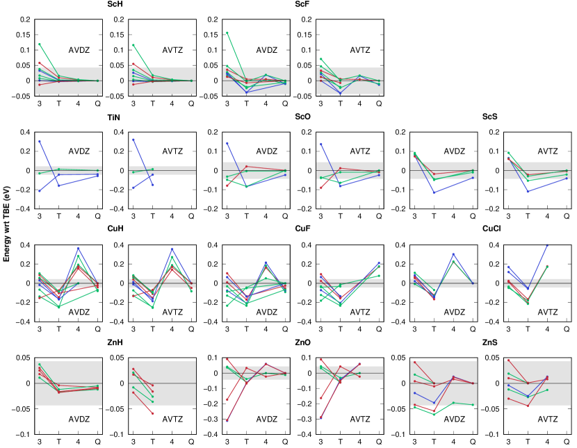
Figure 2: Convergence of the errors in excitation energies (with respect to the TBEs) along the coupled-cluster models (CC3, CCSDT, CC4, and CCSDTQ, denoted by their last digit in the figure), with the aug-cc-pVDZ (AVDZ) and aug-cc-pVTZ (AVTZ) basis set, for $\Sigma$ (red), $\Pi$ (green), and $\Delta$ (blue) excited states of transition metal diatomics. The gray shaded region indicates deviations of $\pm 0.043\text{\,}\mathrm{eV}$ with respect to the TBE.

Table 4: TBEs (in $\mathrm{eV}$) in the aug-cc-pVDZ (AVDZ) and aug-cc-pVTZ (AVTZ) basis sets for the 11 diatomic molecules and the corresponding composite method to generate them.

		aug-cc-pVDZ		aug-cc-pVTZ		literature
Mol.	State	TBE	Method	TBE	Method	Exp.	Th.
ScH	$1\,^{1}\Delta$(4s,3d)	0.606	CCSDTQ	0.672	CCSDTQ	0.519	0.509
	$1\,^{1}\Pi$(4s,3d)	0.820	CCSDTQ	0.875	CCSDTQ	0.670	0.710
	$2\,^{1}\Sigma^{+}$(4s,3d)	1.836	CCSDTQ	1.845	CCSDTQ	1.683	1.703
	$2\,^{1}\Pi$(4s2,3d2)	2.181	CCSDTQ	2.215	CCSDTQ	2.089	2.151
	$1\,^{3}\Delta$(4s,3d)	0.364	CCSDTQ	0.446	CCSDTQ		0.225
	$1\,^{3}\Pi$(4s,3d)	0.565	CCSDTQ	0.621	CCSDTQ		0.430
	$1\,^{3}\Sigma^{+}$(4s,3d)	0.820	CCSDTQ	0.851	CCSDTQ		0.728
	$2\,^{3}\Pi$(4s,3d)	1.832	CCSDTQ	1.817	CCSDTQ		1.852
ScO	$1\,^{2}\Pi$(4s,3d)	2.032	FCI	2.037	FCI	2.057	2.070(6)
	$1\,^{2}\Delta$(4s,3d)	2.107	FCI	2.133	FCI	1.915	1.950(5)
	$2\,^{2}\Sigma^{+}$(4s,3d)	2.563	FCI	2.572	FCI	2.559
	$2\,^{2}\Pi$(2p,4s)	3.550	CCSDTQ	3.570	CCSDTQ
ScF	$1\,^{1}\Delta$(4s,3d)	0.797	FCI	0.903	FCI	0.568	0.478
	$1\,^{1}\Pi$(4s,3d)	1.574	FCI	1.671	FCI/AVDZ + CCSDTQ/AVTZ $-$ CCSDTQ/AVDZ	1.184	1.107
	$2\,^{1}\Sigma^{+}$(4s,3d)	2.346	CCSDTQ	2.404	CCSDTQ	2.527	2.004
	$2\,^{1}\Pi$(4s2,3d2)	2.758	CCSDTQ	2.837	CCSDTQ	2.750	2.521
	$1\,^{3}\Delta$(4s,3d)	0.528	FCI	0.647	FCI	0.242	0.215
	$1\,^{3}\Pi$(4s,3d)	1.037	FCI	1.109	FCI/AVDZ + CCSDT/AVTZ $-$ CCSDT/AVDZ	0.774	0.719
	$1\,^{3}\Sigma^{+}$(4s,3d)	1.401	CCSDTQ	1.459	CCSDTQ/AVDZ + CCSDT/AVTZ $-$ CCSDT/AVDZ		1.073
	$2\,^{3}\Pi$(4s2,3d2)	2.469	CCSDTQ	2.593	CCSDTQ/AVDZ + CCSDT/AVTZ $-$ CCSDT/AVDZ		2.347
ScS	$1\,^{2}\Delta$(4s,3d)	1.300	FCI	1.340	FCI		1.003
	$1\,^{2}\Pi$(4s,3d)	1.495	FCI	1.512	FCI	1.375	1.418
	$2\,^{2}\Sigma^{+}$(4s,3d)	1.590	FCI	1.593	FCI	1.544	1.493
	$2\,^{2}\Pi$(3p,4s)	2.070	CCSDTQ	2.093	CCSDTQ
TiN	$1\,^{2}\Delta$(4s,3d)	1.027	FCI	1.066	FCI	0.934	0.946
	$2\,^{2}\Delta$($\sigma$,3d)	2.008	FCI	2.043	FCI/AVDZ + CCSDT/AVTZ $-$ CCSDT/AVDZ
	$1\,^{2}\Pi$(4s,3d)	2.009	CCSDTQ	1.994	CCSDTQ/AVDZ + CCSDT/AVTZ $-$ CCSDT/AVDZ	2.013	2.01
CuH	$2\,^{1}\Sigma^{+}$(3d,4s)	3.051	FCI	3.080	FCI	2.905	3.009
	$1\,^{1}\Delta$(3d,4s)	3.718	CCSDTQ	3.754	CCSDTQ	3.530
	$1\,^{1}\Pi$(3d,4s)	3.788	FCI	3.829	FCI	3.381	3.406
	$2\,^{1}\Pi$(3d,4s)	5.470	CCSDTQ	5.497	CCSDTQ	5.542	6.035
	$3\,^{1}\Sigma^{+}$(3d,4p)	5.713	CCSDTQ	5.751	CCSDTQ		3.349
	$1\,^{3}\Sigma^{+}$(3d,4s)	2.514	FCI	2.550	FCI/AVDZ + CASPT2/AVTZ $-$ CASPT2/AVDZ	2.418	2.604
	$1\,^{3}\Pi$(3d,4s)	3.522	FCI	3.582	FCI/AVDZ + CASPT2/AVTZ $-$ CASPT2/AVDZ	3.276	3.159
	$1\,^{3}\Delta$(3d,4s)	3.561	CCSDTQ	3.618	CCSDTQ/AVDZ + CASPT2/AVTZ $-$ CASPT2/AVDZ	3.492
	$2\,^{3}\Pi$(3d,4s)	4.762	CCSDTQ	4.817	CCSDTQ/AVDZ + CASPT2/AVTZ $-$ CASPT2/AVDZ		5.209
CuF	$2\,^{1}\Sigma^{+}$(3d,4s)	2.561	FCI	2.572	FCI/AVDZ + CASPT2/AVTZ $-$ CASPT2/AVDZ	2.445	2.31
	$1\,^{1}\Pi$(3d,4s)	2.751	FCI	2.793	FCI/AVDZ + CASPT2/AVTZ $-$ CASPT2/AVDZ	2.512	2.41
	$1\,^{1}\Delta$(3d,4s)	3.285	FCI	3.316	FCI/AVDZ + CASPT2/AVTZ $-$ CASPT2/AVDZ		2.93
	$2\,^{1}\Pi$(3d,4s)	5.914	CCSDTQ	5.933	CCSDTQ/AVDZ + CASPT2/AVTZ $-$ CASPT2/AVDZ
	$1\,^{3}\Sigma^{+}$(3d,4s)	2.017	FCI	2.063	FCI/AVDZ + CASPT2/AVTZ $-$ CASPT2/AVDZ	1.808	1.81
	$1\,^{3}\Pi$(3d,4s)	2.421	FCI	2.471	FCI/AVDZ + CASPT2/AVTZ $-$ CASPT2/AVDZ	2.177	2.17
	$1\,^{3}\Delta$(3d,4s)	2.937	CCSDTQ	2.972	CCSDTQ/AVDZ + CASPT2/AVTZ $-$ CASPT2/AVDZ	2.827	2.65
	$2\,^{3}\Pi$(3d,4s)	5.766	CCSDTQ	5.800	CCSDTQ/AVDZ + CASPT2/AVTZ $-$ CASPT2/AVDZ
CuCl	$2\,^{1}\Sigma^{+}$($\sigma$,4s)	3.004	CCSDTQ	3.065	CCSDTQ/AVDZ + CASPT2/AVTZ $-$ CASPT2/AVDZ	2.848	2.75
	$1\,^{1}\Pi$(3d,4s)	3.008	CCSDTQ	3.092	CCSDTQ/AVDZ + CASPT2/AVTZ $-$ CASPT2/AVDZ	2.861	2.78
	$1\,^{1}\Delta$(3d,4s)	3.540	CCSDTQ	3.479	CCSDTQ/AVDZ + CASPT2/AVTZ $-$ CASPT2/AVDZ		3.20
	$1\,^{3}\Sigma^{+}$($\sigma$,4s)	2.626	CASPT2	2.692	CASPT2	2.352	2.43
	$1\,^{3}\Pi$(3d,4s)	2.661	CASPT2	2.845	CASPT2	2.540	2.62
	$1\,^{3}\Delta$(3d,4s)	3.281	CASPT2	3.229	CASPT2	3.134	3.00
ZnH	$1\,^{2}\Pi$(4s,4p)	2.851	FCI	2.882	FCI	2.90	2.93
	$2\,^{2}\Sigma^{+}$($\sigma$,4s)	4.456	FCI	4.482	FCI/AVDZ + CCSDT/AVTZ $-$ CCSDT/AVDZ	3.42	4.54
	$3\,^{2}\Sigma^{+}$(4s,5s)	5.045	FCI	5.115	FCI	5.09	5.04
	$4\,^{2}\Sigma^{+}$(4s,5p)	5.644	FCI	5.663	FCI/AVDZ + CCSDT/AVTZ $-$ CCSDT/AVDZ		5.70
	$2\,^{2}\Pi$(4s,5p)	6.081	FCI	6.126	FCI		6.09
ZnO	$1\,^{1}\Pi$(2p,4s)	0.771	FCI	0.791	FCI/AVDZ + CC4/AVTZ $-$ CC4/AVDZ	0.615	0.54
	$2\,^{1}\Sigma^{+}$($\sigma$,4s)	3.417	FCI	3.423	FCI/AVDZ + CC4/AVTZ $-$ CC4/AVDZ		3.75
	$1\,^{1}\Delta$(2p,4p)	4.611	CCSDTQ	4.645	CCSDTQ/AVDZ + CC4/AVTZ $-$ CC4/AVDZ		4.90
	$1\,^{1}\Sigma^{-}$(2p,4p)	4.660	CCSDTQ	4.688	CCSDTQ/AVDZ + CC4/AVTZ $-$ CC4/AVDZ		4.76
	$1\,^{3}\Pi$(2p,4s)	0.506	FCI	0.542	FCI/AVDZ + CCSDT/AVTZ $-$ CCSDT/AVDZ	0.305	0.29
	$1\,^{3}\Sigma^{+}$($\sigma$,4s)	1.793	FCI	1.791	FCI/AVDZ + CCSDT/AVTZ $-$ CCSDT/AVDZ	1.875	2.03
ZnS	$1\,^{1}\Pi$(3p,4s)	0.816	FCI	0.814	FCI		0.682
	$2\,^{1}\Sigma^{+}$($\sigma$,4s)	3.622	CCSDTQ	3.641	CCSDTQ/AVDZ + CC4/AVTZ $-$ CC4/AVDZ		3.718
	$1\,^{1}\Delta$(3p,4p)	4.200	CCSDTQ	4.229	CCSDTQ/AVDZ + CC4/AVTZ $-$ CC4/AVDZ		4.279
	$1\,^{1}\Sigma^{-}$(3p,4p)	4.267	CCSDTQ	4.282	CCSDTQ/AVDZ + CC4/AVTZ $-$ CC4/AVDZ		4.239
	$1\,^{3}\Pi$(3p,4s)	0.503	CCSDT	0.546	CCSDT		0.456
	$1\,^{3}\Sigma^{+}$($\sigma$,4s)	2.302	CCSDT	2.306	CCSDT		2.266

^aUnsafe TBE which means error possibly greater than $0.043\text{\,}\mathrm{eV}$. ^b0-0 energy from emission spectroscopy of Ref. Ram and Bernath, 1997. ^c$T_{e}$ energy from MRCI calculations of Ref. Tabet, Adem, and Taher, 2021. ^dVertical energy obtained from the $T_{e}$ chemiluminescence spectroscopy of Refs. Chalek and Gole, 1976, 1977 corrected by the vibrational term, as explained in Ref. Jiang et al., 2021, and averaged over the two spin-orbit components. ^eVertical energy (and statistical uncertainty) from FCIQMC calculations of Ref. Jiang et al., 2021. ^f$T_{e}$ energy from Ref. Huber and Herzberg, 1979. ^g$T_{e}$ energy from emission spectroscopy of Ref. Lebeaultdorget et al., 1994. ^h$T_{e}$ energy from emission spectroscopy of Ref. Shenyavskaya et al., 1993. ⁱ0-0 energy from emission spectroscopy of Ref. Shenyavskaya et al., 1993. ^j$T_{e}$ energy from MRCI+Q calculations of Ref. Langhoff, Bauschlicher, and Partridge, 1988. ^k$T_{e}$ energy from MRCI+Q calculations of Ref. Romeu, Belinassi, and Ornellas, 2018. ^l0-0 energy from emission spectroscopy of Ref. Gengler et al., 2006. ^m$T_{e}$ energy from emission spectroscopy of Ref. Brabaharan, Coxon, and Yamashita, 1985. ⁿ$T_{e}$ energy from MRCI calculations of Ref. Harrison, 1996. ^o$T_{e}$ experimental energy from Ref. Huber and Herzberg, 1979. ^p$T_{e}$ energy from MRCI+Q+DKH calculations of Ref. Xu et al., 2019. ^q0-0 energy from photoelectron spectroscopy of Ref. Calvi, Andrews, and Lineberger, 2007. ^r$T_{e}$ energy from absorption spectroscopy of Ref. Ahmed et al., 1982. ^s$T_{e}$ energy from EOM-CCSD calculations of Ref. Guichemerre, Chambaud, and Stoll, 2002. ^t$T_{e}$ energy from CCSD(T) calculations of Ref. Guichemerre, Chambaud, and Stoll, 2002. ^u0-0 energy from fluorescence spectroscopy of Ref. Delaval et al., 1987. ^v0-0 experimental energy from Ref. Huber and Herzberg, 1979. ^wVertical energy from MS-CASPT2 calculations of Ref. Suo et al., 2017. ^x0-0 energy from photoelectron spectroscopy of Ref. Kim et al., 2001. ^y0-0 energy from MRCI+Q calculations of Ref. Sakellaris, Papakondylis, and Mavridis, 2010. ^z0-0 energy from photoelectron spectroscopy of Ref. Moravec et al., 2001. ^aa0-0 energy from MRCI+Q calculations of Ref. Papakondylis, 2011.

IV.1 ScH and ScF

Out of the eleven transition metal diatomics considered here, the excitation energies of ScH present the fastest convergence along the CC series. Already at the CC3 level, most energies lie within the desired chemical accuracy window ($\pm$$1\text{\,}\mathrm{k}\mathrm{c}\mathrm{a}\mathrm{l}\mathrm{/}\mathrm{m}\mathrm{o}\mathrm{l}$ or $0.043\text{\,}\mathrm{eV}$), as shown in Fig.  2. The largest difference ($0.12\text{\,}\mathrm{eV}$) appears for the fourth singlet state, $2\,^{1}\Pi$(4s²,3d²), which is acceptable since this state has a significant doubly-excited character, making CC3 less efficient. The accuracy is significantly improved at the CCSDT level and beyond. These outcomes are unsurprising, as only 4 electrons are correlated in our (large) frozen core approximation for ScH. Hence, CCSDTQ is equivalent to FCI. In CASPT2 and NEVPT2, all active electrons are correlated, though within a subset of orbitals, and the computed excitation energies deviate more from the TBEs than CC3. There is an average increase of $0.04\text{\,}\mathrm{eV}$ in the TBEs of ScH when going from aug-cc-pVDZ to aug-cc-pVTZ. It is worth mentioning that the $1\,^{3}\Delta$(4s,3d) state of ScH has the lowest TBE of the quest database, of only $0.364\text{\,}\mathrm{eV}$ for the aug-cc-pVDZ basis set and $0.446\text{\,}\mathrm{eV}$ for the aug-cc-pVTZ basis set.

Our vertical TBEs are compatible with the 0-0 experimental energies, Ram and Bernath (1997) the former being higher by $0.13\text{\,}\mathrm{eV}0.21\text{\,}\mathrm{eV}$. The TBEs are also close to the T_e energies calculated at the multireference configuration interaction (MRCI) level, Tabet, Adem, and Taher (2021) appearing higher in energy by $0.06\text{\,}\mathrm{eV}0.22\text{\,}\mathrm{eV}$. The only exception concerns the $2\,^{3}\Pi$(4s,3d) state, whose TBE is lying lower by $-0.03\text{\,}\mathrm{eV}$, possibly related to the occurrence of an avoided crossing with a higher-lying $3\,^{3}\Pi$ state. Tabet, Adem, and Taher (2021)

Moving to ScF, we first note that both $2\,^{1}\Pi$(4s²,3d²) and $2\,^{3}\Pi$(4s²,3d²) excited states are doubly-excited with respect to the ground state. Although the number of active electrons jumps from 4 to 10, the convergence along the CC series remains quite fast, though not on par with the ScH case. CC3 nevertheless delivers chemically accurate excitation energies for most states, except for the $2\,^{3}\Pi$(4s²,3d²) state, whose energy is more overestimated than the others. In fact, third-order methods like CC3 and CCSDT produce fairly accurate excitation energies for the two doubly excited states, with the largest difference to the TBEs produced with CC3 and the aug-cc-pVDZ basis set for the triplet state ($0.156\text{\,}\mathrm{eV}$). This is somewhat surprising given the typically poorer performance of these methods in describing such excited states. Loos et al. (2019) Ramping up to CCSDTQ produces excitation energies too low by only $0.01\text{\,}\mathrm{eV}$ for the states whose TBEs are obtained with CIPSI. Considering the complete set of 11 transition metals investigated here, we find the TBEs to be somewhat larger with the aug-cc-pVTZ basis set, by $0.04\text{\,}\mathrm{eV}$ in average and up to $0.08\text{\,}\mathrm{eV}$. Taking into account the safe TBEs only, ScF shows the most pronounced basis set effects from our set, with the largest increase in the TBEs of $0.124\text{\,}\mathrm{eV}$ for the $2\,^{3}\Pi$(4s²,3d²) state, followed by $0.119\text{\,}\mathrm{eV}$ for the $1\,^{3}\Delta$(4s,3d) state.

The TBEs of ScF can be correlated with the experimental $T_{e}$ and 0-0 energies Lebeaultdorget et al. (1994); Shenyavskaya et al. (1993) as well as with the $T_{e}$ values calculated with MRCI plus Davidson correction (+Q). Langhoff, Bauschlicher, and Partridge (1988) However, the overall largest discrepancies from the current set of transition metal diatomics are seen for this system. Compared to experiment, the TBEs can be lower by $0.12\text{\,}\mathrm{eV}$ [$2\,^{1}\Sigma^{+}$(4s,3d)] or higher by $0.49\text{\,}\mathrm{eV}$ [$1\,^{1}\Pi$(4s,3d)]. This hints at a more significant vibrational relaxation in the excited states than in ScH.

IV.2 CuH, CuF, and CuCl

CuH has 12 active electrons, whereas the halogen-containing compounds CuF and CuCl have 18 in the present (large) frozen core calculations. For some excited states of CuH and CuF, safe TBEs of FCI quality could be attained. For others (and for CuCl), we rely on CCSDTQ or CASPT2 as the TBEs, which are therefore considered unsafe. These systems present strong oscillations in the CC series, having the overall slowest convergence from our set of transition metal compounds. In many cases, detailed below, even CCSDTQ is unable to produce values within the chemically accurate TBEs that stem from FCI calculations. The unfavorable convergence profile is independent of the atom bonded to the Cu, which is the culprit for the observed behavior. The 4s¹ unpaired electron is strongly coupled to the 3d¹⁰ shell, making correlation effects very pronounced in Cu containing systems. This contrasts to the Zn atom, where the additional electron fills the 4s² shell, such that a mean-field approximation is a much more suitable starting point than for strongly correlated Cu atom.

For some states of CuH, the CIPSI calculations yield a small error bar and therefore directly provide trustworthy TBEs. Accounting for these states only, the average absolute errors are smaller with CCSDTQ ($0.05\text{\,}\mathrm{eV}$) than with CASPT2 ($0.12\text{\,}\mathrm{eV}$), besides being more systematic with the former method. We thus expect CCSDTQ to perform similarly better than CASPT2 for the other excited states, where FCI is unattainable, and for this reason, CCSDTQ is the method of choice for obtaining their TBEs. Given the systematic underestimation of CCSDTQ with respect to the available FCI estimates, by $0.02\text{\,}\mathrm{eV}0.08\text{\,}\mathrm{eV}$ with the aug-cc-pVDZ basis set, the true TBEs are probably greater (by a comparable amount) than those obtained with CCSDTQ. The same reasoning holds for CuF. The average error for the 5 states where FCI/aug-cc-pVDZ estimates are accessible is smaller for CCSDTQ ($0.06\text{\,}\mathrm{eV}$) than for CASPT2 ($0.12\text{\,}\mathrm{eV}$), the former method underestimating the TBEs by $0.02\text{\,}\mathrm{eV}0.09\text{\,}\mathrm{eV}$. The CCSDTQ results for the remaining 3 excited states thus provide our TBEs, which are in turn expected to be a bit too low. When only CCSDT results are available (which is the case of the triplet states of CuCl), we rely on CASPT2 for the TBEs, based on the same argument. Despite the missing FCI estimates for CuCl, the similarity between its excited states and those of CuH and CuF makes us believe that CCSDTQ would also be more accurate than CASPT2 for this system. However, we note that the CC error formally increases more rapidly with the number of electrons than the CASPT2 one. Enlarging the basis set from aug-cc-pVDZ to aug-cc-pVTZ affects all TBEs of CuH quite similarly, which increase by $0.03\text{\,}\mathrm{eV}0.06\text{\,}\mathrm{eV}$, averaging at $0.04\text{\,}\mathrm{eV}$. For CuF, they increase by $0.01\text{\,}\mathrm{eV}0.05\text{\,}\mathrm{eV}$, with an average of $0.03\text{\,}\mathrm{eV}$.

For the three Cu containing compounds, the profile of the CC convergence is similar for most states. CC3 provides fairly decent excitation energies (typically within $0.2\text{\,}\mathrm{eV}$ of the TBEs), considering its relatively low computational cost. CCSDT often becomes less accurate and underestimates the TBEs, which are then overestimated by CC4. Overall, CC3 is more accurate (and cheaper) than the higher-order CCSDT and CC4 models. CCSDTQ is probably enough to achieve an accuracy of $0.1\text{\,}\mathrm{eV}$. To ensure chemical accuracy ($0.043\text{\,}\mathrm{eV}$), at least pentuple excitations should likely be accounted for in CC models.

The three species present the overall very large discrepancies between CC4 and CCSDTQ and between CC3 and CCSDT, from $0.2\text{\,}\mathrm{eV}0.3\text{\,}\mathrm{eV}$. This is considerably more than usually observed for typical excited states of organic species. Loos et al. (2018, 2020c, 2021b, 2022) They also showed the overall largest differences between the TBEs and the various CC models. For instance, the $1\,^{1}\Pi$(3d,4s) state of CuH is one of the most challenging of our set. With the aug-cc-pVDZ basis set, the TBE of $3.788\text{\,}\mathrm{eV}$ obtained with FCI is considered safe. This TBE presents the largest difference to CCSDT ($3.537\text{\,}\mathrm{eV}$), of $-0.251\text{\,}\mathrm{eV}$, and to CC4 ($4.072\text{\,}\mathrm{eV}$), of $0.284\text{\,}\mathrm{eV}$, and the second largest difference to CCSDTQ ($3.707\text{\,}\mathrm{eV}$), of $-0.081\text{\,}\mathrm{eV}$. For the aug-cc-pVTZ basis set, the same state also presents the largest energy difference obtained with CCSDTQ ($3.746\text{\,}\mathrm{eV}$) and the safe TBE from FCI ($3.829\text{\,}\mathrm{eV}$), of $-0.083\text{\,}\mathrm{eV}$.

Despite these difficulties in the convergence of the CC series, there is overall good agreement between our TBEs and the previous results for CuH, CuF, and CuCl. Starting with CuH, our TBEs appear $-0.04\text{\,}\mathrm{eV}0.45\text{\,}\mathrm{eV}$ relative to the $T_{e}$ experimental energies Huber and Herzberg (1979) [0-0 energy in the case of the $1\,^{3}\Sigma^{+}$(3d,4s) state Calvi, Andrews, and Lineberger (2007)]. They are also consistent with MRCI+Q calculations (with relativistic effects), except for the $3\,^{1}\Sigma^{+}$(3d,4p) state, much higher in energy in all our calculations (TBE of $5.751\text{\,}\mathrm{eV}$ with the larger basis set) than in the previous one ($3.349\text{\,}\mathrm{eV}$). Xu et al. (2019) This state has also been assigned as $3\,^{1}\Sigma^{+}$ in Ref. Xu et al., 2019, so the reason for this discrepancy is unclear.

The 4 states of CuF for which safe TBEs can be compared with experiment, Ahmed et al. (1982) appear higher in energy than the experimentally obtained $T_{e}$ values from $0.13\text{\,}\mathrm{eV}0.29\text{\,}\mathrm{eV}$. They are also consistent with previous CCSD(T) and EOM-CCSD calculations. Guichemerre, Chambaud, and Stoll (2002) Our TBEs for the $1\,^{3}\Delta$(3d,4s) state are close to and in-between the experimental Ahmed et al. (1982) and EOM-CCSD results. Guichemerre, Chambaud, and Stoll (2002) For the $2\,^{1}\Pi$(3d,4s) and $2\,^{3}\Pi$(3d,4s) excited states, there is, to our knowledge, no previous data to compare our results with.

Our TBEs for CuCl are also consistent with the 0-0 experimental values, Delaval et al. (1987) which are overestimated by $0.09\text{\,}\mathrm{e}\mathrm{V}0.34\text{\,}\mathrm{e}\mathrm{V}$. There is also a correspondence between our TBEs and the $T_{e}$ values obtained from CCSD(T) calculations for the 3 triplet states Guichemerre, Chambaud, and Stoll (2002) and from EOM-CCSD calculations for the 3 singlet states, Guichemerre, Chambaud, and Stoll (2002) though with quite larger differences in general, from $0.23\text{\,}\mathrm{eV}0.40\text{\,}\mathrm{eV}$.

IV.3 ZnO and ZnS

ZnO and ZnS have 18 active electrons in our large frozen core approximation, the largest number in our set of transition metal diatomics (along with CuF and CuCl). Despite that, the convergence along the CC series can be considered satisfactory, being far superior to the case of Cu containing compounds.

The CC estimates for both the $1\,^{1}\Pi$(2p,4s) and $1\,^{3}\Pi$(2p,4s) excited states of ZnO always fall within the chemically accurate region, even with CC3. Meanwhile, at least CCSDT is needed to reach the same level of accuracy for the $2\,^{1}\Sigma^{+}$($\sigma$,4s) state, whereas the $1\,^{1}\Delta$(2p,4p) and $1\,^{1}\Sigma^{-}$(2p,4p) states are more challenging and would require at least CCSDTQ, which provides our (unsafe) TBEs. For the latter two excited states, CC3 produces excitation energies largely underestimated, by ca. $0.3\text{\,}\mathrm{eV}$. CCSDT significantly reduces the errors, bringing the energies from $0.05\text{\,}\mathrm{eV}0.07\text{\,}\mathrm{eV}$ below their TBEs. However, CC4 does not lead to further improvement, as it overestimates the TBEs by around the same amount, $0.06\text{\,}\mathrm{eV}$. CCSDTQ is taken as the TBE, but it is not clear whether this level of theory is enough to achieve chemical accuracy for these two excited states.

Our TBEs for ZnO are consistent with the previous reports on the 0-0 energies. Kim et al. (2001); Moravec et al. (2001); Sakellaris, Papakondylis, and Mavridis (2010) For the lowest singlet [$1\,^{3}\Pi$(2p,4s)] and triplet [$1\,^{3}\Pi$(2p,4s)] excited states, they exceed the experimental values Kim et al. (2001); Moravec et al. (2001) by $0.18\text{\,}\mathrm{eV}$ and $0.24\text{\,}\mathrm{eV}$, respectively, and MRCI+Q calculations Sakellaris, Papakondylis, and Mavridis (2010) by $0.25\text{\,}\mathrm{eV}$ (both states). These differences can be explained by the potential energy curves reported in Ref. Sakellaris, Papakondylis, and Mavridis, 2010, which indicate considerably stretched equilibrium geometries for these two excited states (more so for the $1\,^{3}\Pi$(2p,4s) state). Conversely, our TBE for the $1\,^{3}\Sigma^{+}$($\sigma$,4s) state is smaller than the experimental and the MRCI+Q 0-0 energy, by $0.08\text{\,}\mathrm{eV}$ and $0.24\text{\,}\mathrm{eV}$, respectively. Here, ground- and excited-state bond distances are actually similar, and the underestimated TBE probably indicates that the excited-state zero-point vibrational energy is greater than the ground-state one. Sakellaris, Papakondylis, and Mavridis (2010) There is no experimental data for the 3 higher-lying states, though our TBEs are systematically lower (by $0.07\text{\,}\mathrm{eV}0.33\text{\,}\mathrm{eV}$) than the values obtained in the MRCI+Q calculations. Sakellaris, Papakondylis, and Mavridis (2010)

For ZnS, CC3 is able to provide excitation energies with virtual chemical accuracy. It is rather surprising that it performs significantly better than for ZnO, considering that both systems share the same excited states character and number of active electrons. The $2\,^{1}\Sigma^{+}$($\sigma$,4s) state is very well described already at the CC3 level, and the energy computed at higher-order CC levels fluctuates around the TBE (corresponding to the CCSDTQ value for this state). Despite the proximity between the CCSDTQ and FCI results, the residual statistical uncertainty of the latter prevents us from claiming this TBE to be safe. For the two triplet excited states, $1\,^{3}\Pi$(3p,4s) and $1\,^{3}\Sigma^{+}$($\sigma$,4s), CCSDT represents our TBEs, which are also considered unsafe. CCSDT slightly but systematically decreases the excitation energies of all states, which worsens the comparison with the TBEs for the $1\,^{1}\Pi$(3p,4s), $1\,^{1}\Delta$(3p,4p), and $1\,^{1}\Sigma^{-}$(3p,4p) states. For the latter two, one needs CC4 to obtain a significant reduction in the errors.

The behavior of the first singlet excited state of ZnS, $1\,^{1}\Pi$(3p,4s), stands out. Along the CC series (CC3, CCSDT, CC4, and CCSDTQ), its aug-cc-pVDZ excitation energy oscillates between $0.755\text{\,}\mathrm{eV}$ and $0.778\text{\,}\mathrm{eV}$, a narrow interval of $0.023\text{\,}\mathrm{eV}$. However, the apparent convergence can be ruled out with our FCI estimate of $0.816\text{\,}\mathrm{eV}$, which represents our TBE. This value lies $0.042\text{\,}\mathrm{eV}$ above the CCSDTQ result and is significantly greater than the $0.003\text{\,}\mathrm{eV}$ statistical uncertainty of the FCI result. A similar trend is observed for the aug-cc-pVTZ basis set, though with a substantially smaller gap ($0.013\text{\,}\mathrm{eV}$) between FCI and CC4 (CCSDTQ is beyond computational reach). The convergence profile of the CC series is overall similar with both basis sets, somewhat less so than observed for ZnO. The TBEs of both ZnO and ZnS are slightly larger with the aug-cc-pVTZ basis set, by $0.02\text{\,}\mathrm{eV}$ in average.

Our computed TBEs for ZnS are once again close to previous MRCI+Q results for the 0-0 energies, Papakondylis (2011) with differences between $-0.08\text{\,}\mathrm{eV}0.13\text{\,}\mathrm{eV}$, and the TBEs appear lower in energy for 2 out of the 6 excited states, $2\,^{1}\Sigma^{+}$($\sigma$,4s) and $1\,^{1}\Delta$(3p,4p). To the best of our knowledge, ZnS is the single compound investigated here for which there is no experimental excited-state data.

IV.4 ScO and ScS

Both ScO and ScS are radicals having 9 active electrons in our calculations. For most states, the CC series quickly converges to the TBEs, though less than in the closed-shell ScH and ScF derivatives. In particular, the CC series is overall faster for ScF than for ScO. This reflects the impact of the additional electron from the F atom (compared with the O atom) closing the 3p shell.. The effect is small however, when compared to the case where the single electron difference is associated with the transition metals, as shown earlier for CuH and ZnH.

The $1\,^{2}\Delta$(4s,3d) excited states of both ScO and ScS are the most challenging for these systems. CC3 and CCSDT display deviations of around $0.1\text{\,}\mathrm{eV}$ with respect to the TBE, by either overestimating or underestimating it, respectively. The description of these excited states only becomes chemically accurate at the CCSDTQ level. For both species, the CC convergence profile is quite insensitive to the basis set.

Our TBE for the $1\,^{2}\Pi$(4s,3d) state of ScO ($2.037\text{\,}\mathrm{eV}$) very closely matches both the vertical excitation energy obtained with accurate FCI quantum Monte Carlo (FCIQMC) calculations ($2.070\text{\,}\mathrm{eV}$), Jiang et al. (2021) and the estimated experimental vertical energy ($2.057\text{\,}\mathrm{eV}$), based on the $T_{e}$ of Refs. Chalek and Gole, 1976, 1977 corrected for vibrational effect according to Ref. Jiang et al., 2021. In turn, the differences are greater for the $1\,^{2}\Delta$(4s,3d) state, with our TBE of $2.133\text{\,}\mathrm{eV}$ appearing higher in energy than both the FCIQMC one ($1.950\text{\,}\mathrm{eV}$) Jiang et al. (2021) and the estimated experimental vertical energy ($1.915\text{\,}\mathrm{eV}$). Chalek and Gole (1976, 1977); Jiang et al. (2021) Our TBEs place the $1\,^{2}\Delta$(4s,3d) state higher in energy than the $1\,^{2}\Pi$(4s,3d) state, in contrast to the available experimental and theoretical results. This is not too serious, however, as their energy gap is small, probably around $0.1\text{\,}\mathrm{eV}$. As for the $2\,^{2}\Sigma^{+}$(4s,3d) state, our TBE differs from the experimental $T_{e}$ value Huber and Herzberg (1979) by $0.013\text{\,}\mathrm{eV}$ only. There is no previous data for the higher-lying $2\,^{2}\Pi$(2p,4s) excited state as far as we know.

The TBEs for the $1\,^{2}\Pi$(4s,3d) and $2\,^{2}\Sigma^{+}$(4s,3d) excited states of ScS are consistent with both the available 0-0 experimental values Gengler et al. (2006) and with MRCI+Q $T_{e}$ calculations, Romeu, Belinassi, and Ornellas (2018) being higher in energy by $0.05\text{\,}\mathrm{eV}0.14\text{\,}\mathrm{eV}$. Whereas the lowest-lying excited state of ScS, $1\,^{2}\Delta$(4s,3d) remains to be observed experimentally, our TBE is higher than its MRCI+Q counterpart Romeu, Belinassi, and Ornellas (2018) by $0.34\text{\,}\mathrm{eV}$, a larger difference than for the two higher-lying excited states. At least to some extent, this can be explained by the larger equilibrium bond distance of the first excited state, based on the MRCI+Q potential energy curves. Romeu, Belinassi, and Ornellas (2018)

IV.5 TiN and ZnH

TiN and ZnH are radical species, having 9 and 13 active electrons in our calculations, respectively. The first excited state of TiN, $1\,^{2}\Delta$(4s,3d), shows a slow convergence along the CC series. Compared to the TBE, its excitation energy is significantly overestimated at the CC3 level ($0.30\text{\,}\mathrm{eV}0.32\text{\,}\mathrm{eV}$, depending on the basis set), becoming underestimated at CCSDT level ($0.15\text{\,}\mathrm{eV}0.16\text{\,}\mathrm{eV}$). The error further decreases with CCSDTQ, though not enough to reach chemical accuracy, as the computed energy appears $0.06\text{\,}\mathrm{eV}$ below the TBE with the aug-cc-pVDZ basis set. For the next state, $2\,^{2}\Delta$($\sigma$,3d), CC3 also starts off with a large error, this time undeshooting the TBE by $0.18\text{\,}\mathrm{eV}0.21\text{\,}\mathrm{eV}$. With the aug-cc-pVDZ basis set, the excitation energy obtained with CCSDT ($1.965\text{\,}\mathrm{eV}$) and CCSDTQ ($1.969\text{\,}\mathrm{eV}$) varies by only $0.004\text{\,}\mathrm{eV}$, suggesting fairly converged results. However, the TBE of $2.008\text{\,}\mathrm{eV}$ (obtained with FCI) still lies $0.039\text{\,}\mathrm{eV}$ above the CCSDTQ energy. For both $1\,^{2}\Delta$(4s,3d) and $2\,^{2}\Delta$($\sigma$,3d) states of TiN, excitations beyond quadruples seem needed to effectively reach chemical accuracy. The higher-lying excited state, $1\,^{2}\Pi$(4s,3d), displays a very small error already at the CC3 level, becoming tinier at the higher CC levels. We further notice that the convergence profile up to CCSDT is quite insensitive to the choice of basis sets.

The TBEs for TiN are very close to the available $T_{e}$ energies obtained experimentally Brabaharan, Coxon, and Yamashita (1985) and with MRCI calculations. Harrison (1996) Compared to the previously reported values, the TBE for the $1\,^{2}\Delta$(4s,3d) state is larger by $0.12\text{\,}\mathrm{eV}0.13\text{\,}\mathrm{eV}$, whereas for the $1\,^{2}\Pi$(4s,3d) state, it is smaller by $0.07\text{\,}\mathrm{eV}$. The $2\,^{2}\Delta$($\sigma$,3d) excited state, although very close lying in energy to the $1\,^{2}\Pi$(4s,3d) state, has not been considered in the previous experimental and theoretical studies.

ZnH presents one of the most favorable CC convergence profiles with the aug-cc-pVDZ basis set. CC3 produces chemically accurate excitation energies with a slight overestimation with the double-$\zeta$ basis set. CCSDT is very accurate with the aug-cc-pVDZ basis set (within $0.02\text{\,}\mathrm{eV}$ of the TBEs), but slightly less with the aug-cc-pVTZ basis set (with deviations up to $0.06\text{\,}\mathrm{eV}$). That is a sizeable basis set effect not seen in the other transition metal diatomics. CCSDTQ underestimates the TBEs by $0.005\text{\,}\mathrm{eV}0.015\text{\,}\mathrm{eV}$ only.

There is very good agreement between the TBEs of ZnH and the vertical excitation energies computed with multistate CASPT2 (MS-CASPT2) calculations, Suo et al. (2017) with average absolute deviations of $0.06\text{\,}\mathrm{eV}$ for the five excited states considered here. Our CASPT2 results are even more accurate, with average absolute deviations of $0.03\text{\,}\mathrm{eV}$. The TBEs are also very close to the available experimental data Huber and Herzberg (1979) for the $1\,^{2}\Pi$(4s,4p) and $3\,^{2}\Sigma^{+}$(4s,5s) 0-0 energies, respectively underestimated and overestimated by only $0.02\text{\,}\mathrm{eV}$. A much larger deviation of $1.06\text{\,}\mathrm{eV}$ is seen for the $2\,^{2}\Sigma^{+}$($\sigma$,4s) state, probably reflecting its more stretched equilibrium bond distance. Huber and Herzberg (1979); Jamorski et al. (1994); Suo et al. (2017)

IV.6 Global statistics

We computed the mean signed error (MSE), mean absolute error (MAE), and root-mean-square error (RMSE), gathered in Table 5, for both CC and multiconfigurational methods considered here. They were evaluated with respect to the TBEs displayed in Table 4, including results for both basis sets and excluding the unsafe excited states (having errors potentially greater than $0.043\text{\,}\mathrm{eV}$). Figure 3 shows the corresponding distribution of errors in the excitation energies. We collect the results from both basis sets because the main trends, discussed in the following, are rather insensitive to the choice of the basis set. The individual results for each one can be found in the supporting information.

Table 5: Mean signed error (MSE), mean absolute error (MAE), and root-mean-square error (RMSE), in units of eV, with respect to the TBEs for all the states assigned as safe in Table 4.

Method	#	MSE	MAE	RMSE
CC3	$90$	$+0.02$	$0.06$	$0.09$
CCSDT	$90$	$-0.05$	$0.06$	$0.09$
CC4	$34$	$+0.05$	$0.05$	$0.10$
CCSDTQ	$63$	$-0.02$	$0.02$	$0.03$
CASPT2 (IPEA)	$90$	$-0.08$	$0.12$	$0.16$
CASPT2 (no IPEA)	$90$	$-0.11$	$0.13$	$0.17$
PC-NEVPT2	$64$	$-0.08$	$0.12$	$0.16$
SC-NEVPT2	$64$	$-0.07$	$0.14$	$0.18$

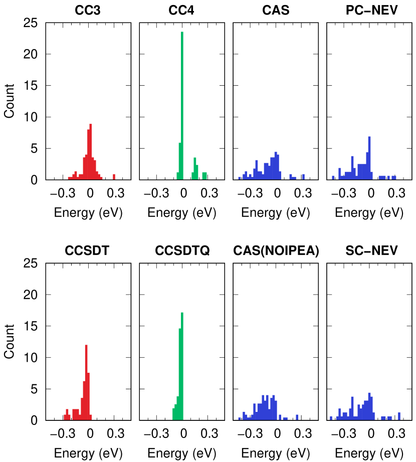
Figure 3: Distribution of the errors in excitation energies with respect to the safe TBEs of Table 4, with corresponding statistical errors presented in Table 5, where CAS and NEV stand for CASPT2 and NEVPT2, respectively.

CC3 displays a fairly normal distribution of errors, centered around zero (MSE of $0.02\text{\,}\mathrm{eV}$) and the associated MAE is $0.06\text{\,}\mathrm{eV}$ only. By fully accounting for the triple excitations, CCSDT produces a negatively skewed distribution, with the MSE moving further away from zero ($-0.05\text{\,}\mathrm{eV}$), and the MAE remaining at $0.06\text{\,}\mathrm{eV}$. Moving to CC4 only slightly reduces the MAE to $0.05\text{\,}\mathrm{eV}$, whereas the underlying distribution becomes positively skewed with a MSE of $0.05\text{\,}\mathrm{eV}$. CCSDTQ significantly reduces the errors, with a MAE of only $0.02\text{\,}\mathrm{eV}$ and a somewhat negatively skewed distribution with a MSE of $-0.02\text{\,}\mathrm{eV}$. These very small errors would be expected, given that one-third of our safe TBEs stem from CCSDTQ calculations. Excluding these TBEs slightly shifts the MAE to $0.03\text{\,}\mathrm{eV}$ and the MSE to $-0.03\text{\,}\mathrm{eV}$.

In turn, the four different multiconfigurational approaches globally yield less accurate excitation energies than the CC models. The errors are quite comparable among them, with the MAEs lying between $0.12\text{\,}\mathrm{eV}0.14\text{\,}\mathrm{eV}$, MSEs of $-0.11\text{\,}\mathrm{eV}-0.08\text{\,}\mathrm{eV}$, and negatively skewed distribution of the errors for all methods. CASPT2 with the IPEA shift is the most accurate out of the four, yet by a small margin. The effect of the IPEA shift is rather small, decreasing the MAE by $0.01\text{\,}\mathrm{eV}$ and making the MSE less negative by $0.03\text{\,}\mathrm{eV}$. Similarly, the errors of PC-NEVPT2 and SC-NEVPT2 differ by no more than $0.02\text{\,}\mathrm{eV}$. The comparable statistics obtained with the multiconfigurational methods endorses the choice of active spaces.

The accuracy of the tested CC models is overall independent of the basis set and is comparable for singlets, doublets, and triplets. They are also similar across the different spatial symmetries, except for CC3, which performs better for $\Sigma$ and $\Pi$ (MAE of $0.05\text{\,}\mathrm{eV}$) than for $\Delta$ (MAE of $0.09\text{\,}\mathrm{eV}$) excited states. In contrast, the multiconfigurational methods display more pronounced differences, improving towards states of lower angular momentum. CASPT2/PC-NEVPT2 show a MAE of $0.21\text{\,}\mathrm{eV}$/$0.20\text{\,}\mathrm{eV}$ for $\Delta$ states, decreasing to $0.12\text{\,}\mathrm{eV}$/$0.10\text{\,}\mathrm{eV}$ for $\Pi$ states, and down to $0.08\text{\,}\mathrm{eV}$/$0.09\text{\,}\mathrm{eV}$ for $\Sigma$ states. The multiconfigurational methods also deliver somewhat more accurate results for triplet than for singlet excited states, with respective MAEs of $0.12\text{\,}\mathrm{eV}$ and $0.15\text{\,}\mathrm{eV}$ according to CASPT2, and of $0.11\text{\,}\mathrm{eV}$ and $0.14\text{\,}\mathrm{eV}$ based on PC-NEVPT2. Finally, the results are closer to the TBEs with the smaller basis set. Both CASPT2 and PC-NEVPT2 have a MAE of $0.11\text{\,}\mathrm{eV}$ with the aug-cc-pVDZ basis set, which increases to $0.14\text{\,}\mathrm{eV}$ with the larger aug-cc-pVTZ basis set. The same trends concerning basis sets and spatial/spin symmetries are observed with or without the IPEA shift and also for both PC-NEVPT2 and SC-NEVPT2.

It is interesting to compare the statistical errors for the present transition metal compounds with those for organic molecules obtained in the previous sets of the quest database. For the transition metals, CC3 offers a MAE of $0.06\text{\,}\mathrm{eV}$. Although acceptable for most purposes, such error is greater than those previously found for other types of excited states. By comparing with previous quest subsets for which CCSDTQ or FCI TBEs are available, we find that the MAEs of CC3 become progressively smaller for the radicals of quest#4 Loos et al. (2020c) ($0.05\text{\,}\mathrm{eV}0.06\text{\,}\mathrm{eV}$), the small molecules of quest#1 Loos et al. (2018) ($0.03\text{\,}\mathrm{eV}$), and the exotic molecules of quest#4 Loos et al. (2020c) ($0.01\text{\,}\mathrm{eV}$). Even though CC3 performs very well in absolute terms, the MAEs for each type of transition span a range of $0.01\text{\,}\mathrm{eV}0.06\text{\,}\mathrm{eV}$, which is large in relative terms. The accuracy is excellent for typical transitions of organic molecules, though less so for radicals and for transitions whose states present pronounced multiconfigurational character, as the transition metal derivatives surveyed here.

A similar comparison of CASPT2 and NEVPT2 reveals a different picture. For the transition metal diatomics, the MAE of $0.12\text{\,}\mathrm{eV}0.14\text{\,}\mathrm{eV}$ is virtually the same as obtained for the medium-sized organic molecules of quest#3 Loos et al. (2020b) with NEVPT2 ($0.13\text{\,}\mathrm{eV}$). Even though these results certainly depend on the choice of active space, they highlight the versatility of CASPT2 and NEVPT2 methods in handling excited states with varying multiconfigurational characters while providing very similar levels of accuracy. This contrasts with the case of CC3, whose accuracy is more dependent on the type of transitions. However, even for the challenging transitions in transition metal diatomics, the single-reference CC3 still outperforms the multiconfigurational alternatives. Interestingly, the IPEA shift has apparently a smaller impact on the transition metal diatomics than on organic systems. Sarkar et al. (2022); Boggio-Pasqua, Jacquemin, and Loos (2022) In addition, the CASPT2 and NEVPT2 excitation energies are generally very similar for the systems considered here. These observations further support our active spaces choices.

V Conclusion

We have presented highly-accurate vertical excitation energies for 67 excited states of 11 transition metal diatomic molecules, comprising 4 different fourth-row elements (Sc, Ti, Cu, and Zn). To this end, we employed state-of-the-art excited-state methods, including selected CI, high-order equation-of-motion CC (CC3, CCSDT, CC4, and CCSDTQ), and multiconfigurational (CASPT2 and NEVPT2) methods. These calculations allowed us to provide non-relativistic theoretical best estimates (based on the aug-cc-pVDZ and aug-cc-pVTZ basis sets) for the excitation energies of 67 states, 45 of which should be chemically accurate (errors less than $0.043\text{\,}\mathrm{eV}$ or $1\text{\,}\mathrm{k}\mathrm{c}\mathrm{a}\mathrm{l}\mathrm{/}\mathrm{m}\mathrm{o}\mathrm{l}$). These TBEs were compared with previous experimental and theoretical results. This contribution establishes the eighth subset of the quest database, the first comprising transition metals.

The convergence of the CC series toward the TBE shows a pronounced dependence on the system. It is quite favorable for the Sc-containing species, ScH, ScF, ScO, and ScS (somewhat less so for the latter two, open-shell radicals), followed by the Zn-containing species, ZnH, ZnO, and ZnS, although ZnO presents a few challenging excited states. TiN presents a slower convergence profile, whereas the Cu-containing compounds, CuH, CuF, and CuCl proved to be the most challenging systems from the present set. This trend can be rationalized based on the occupancy of the 3d and 4s shells of the transition atom. Moving one position towards the center of the periodic table (from Sc to Ti and from Zn to Cu) increases the half-filled character of the shells, making the electronic correlation problem harder to tackle.

Despite the challenging multiconfigurational character of many excited states, CC3 performs surprisingly well, with a MAE of $0.06\text{\,}\mathrm{eV}$, not significantly more than observed for transitions of small organic systems ($0.01\text{\,}\mathrm{eV}0.06\text{\,}\mathrm{eV}$). The higher-order CCSDT and CC4 levels produce comparable MAEs, although their corresponding error distributions are negatively and positively skewed, respectively. A further reduction in the errors only comes at the CCSDTQ level, with a MAE of $0.02\text{\,}\mathrm{eV}$. In turn, the multiconfigurational methods are less accurate than CC3, with MAEs of $0.12\text{\,}\mathrm{eV}0.14\text{\,}\mathrm{eV}$. Yet, we found quite consistent results with both forms of NEVPT2 and CASPT2, and a small effect introduced by the IPEA shift. Overall, if an accuracy of around $0.1\text{\,}\mathrm{eV}0.2\text{\,}\mathrm{eV}$ is acceptable, CC3 would be recommended. Otherwise, CCSDTQ is needed to achieve chemical accuracy, though it is still insufficient for the most difficult cases.

While the current reference vertical energies offer significant value, it is important to note that they do not take into account relativistic effects. Saue et al. (2020) Incorporating such effects, which can significantly affect vertical transition energies in some cases, would be both a logical and formidable undertaking that holds substantial potential value for the electronic structure community.

Supporting Information

Additional statistical measures for each basis set and various types of excited states, comparison between small and large frozen-core calculations, additional CASSCF, CASPT2 (with and without IPEA shift), and (partially- and strongly-contracted) NEVPT2 data, as well as the detailed description and specification of the active space for each molecule and each transition.

References

- Khomskii (2014) D. I. Khomskii, Transition Metal Compounds (Cambridge University Press, 2014).
- Trautwein (1997) A. Trautwein, Bioinorganic Chemistry: Transition Metals in Biology and Their Coordination Chemistry (Wiley-VCH, 1997).
- Askerka, Brudvig, and Batista (2016) M. Askerka, G. W. Brudvig, and V. S. Batista, Acc. Chem. Res. 50, 41 (2016).
- Ebert (1996) H. Ebert, Rep. Prog. Phys. 59, 1665 (1996).
- van Oudenaarden et al. (1998) A. van Oudenaarden, M. H. Devoret, Y. V. Nazarov, and J. E. Mooij, Nature 391, 768 (1998).
- Gerhard et al. (2010) L. Gerhard, T. K. Yamada, T. Balashov, A. F. Takács, R. J. H. Wesselink, M. Däne, M. Fechner, S. Ostanin, A. Ernst, I. Mertig, and W. Wulfhekel, Nat. Nanotechnol.) 5, 792 (2010).
- Melius (1976) C. F. Melius, Chem. Phys. Lett. 39, 287 (1976).
- (8) C. Bolm, C. Palazzi, and O. Beckmann, in Transition Metals for Organic Synthesis (Wiley-VCH Verlag GmbH) pp. 267–274.
- Ma et al. (2021) C. Ma, P. Fang, D. Liu, K.-J. Jiao, P.-S. Gao, H. Qiu, and T.-S. Mei, Chem. Sci. 12, 12866 (2021).
- García-Melchor et al. (2013) M. García-Melchor, A. A. C. Braga, A. Lledós, G. Ujaque, and F. Maseras, Acc. Chem. Res. 46, 2626 (2013).
- Guest et al. (2015) D. Guest, V. H. M. da Silva, A. P. de Lima Batista, S. M. Roe, A. A. C. Braga, and O. Navarro, Organometallics 34, 2463 (2015).
- Sperger et al. (2015) T. Sperger, I. A. Sanhueza, I. Kalvet, and F. Schoenebeck, Chem. Rev. 115, 9532 (2015).
- Bernardi et al. (1990) F. Bernardi, S. De, M. Olivucci, and M. A. Robb, J. Am. Chem. Soc. 112, 1737 (1990).
- Klessinger and Michl (1995) M. Klessinger and J. Michl, “Excited states and photochemistry of organic molecules,” (VCH, New York, 1995).
- Robb et al. (2007) M. A. Robb, M. Garavelli, M. Olivucci, and F. Bernardi, “A Computational Strategy for Organic Photochemistry,” in Reviews in Computational Chemistry, edited by K. B. Lipkowitz and D. B. Boyd (John Wiley & Sons, Inc., Hoboken, NJ, USA, 2007) pp. 87–146.
- Delgado et al. (2010) J. L. Delgado, P.-A. Bouit, S. Filippone, M. Herranz, and N. Martín, Chem. Comm. 46, 4853 (2010).
- Olivucci (2010) M. Olivucci, Computational Photochemistry (Elsevier Science, Amsterdam; Boston (Mass.); Paris, 2010).
- Twilton et al. (2017) J. Twilton, C. Le, P. Zhang, M. H. Shaw, R. W. Evans, and D. W. C. MacMillan, Nat. Rev. Chem. 1, 0052 (2017).
- Geneaux et al. (2019) R. Geneaux, H. J. B. Marroux, A. Guggenmos, D. M. Neumark, and S. R. Leone, Phil. Trans. R. Soc. A. 377, 20170463 (2019).
- Haglund (2007) R. F. Haglund, in Laser Ablation and its Applications (Springer US, 2007) pp. 185–213.
- Bokarev and Kühn (2019) S. I. Bokarev and O. Kühn, WIREs Comput. Mol. Sci. 10, e1433 (2019).
- Harrison (2000) J. F. Harrison, Chem. Rev. 100, 679 (2000).
- Harvey (2006) J. N. Harvey, Annu. Rep. Prog. Chem., Sect. C: Phys. Chem. 102, 203 (2006).
- Zhao and Truhlar (2006) Y. Zhao and D. G. Truhlar, J. Chem. Phys. 124, 224105 (2006).
- Sperger, Sanhueza, and Schoenebeck (2016) T. Sperger, I. A. Sanhueza, and F. Schoenebeck, Acc. Chem. Res. 49, 1311 (2016).
- Santoro et al. (2016) S. Santoro, M. Kalek, G. Huang, and F. Himo, Acc. Chem. Res. 49, 1006 (2016).
- Friesner and Jerome (2017) R. A. Friesner and S. V. Jerome, Coord. Chem. Rev. 344, 205 (2017).
- Hait et al. (2019) D. Hait, N. M. Tubman, D. S. Levine, K. B. Whaley, and M. Head-Gordon, J. Chem. Theory Comput. 15, 5370 (2019).
- Roos et al. (1996a) B. O. Roos, K. Andersson, M. P. Fulscher, P.-A. Malmqvist, and L. Serrano-Andrés, “Multiconfigurational perturbation theory: Applications in electronic spectroscopy,” (Wiley, New York, 1996) pp. 219–331.
- Piecuch et al. (2002) P. Piecuch, K. Kowalski, I. S. O. Pimienta, and M. J. Mcguire, Int. Rev. Phys. Chem. 21, 527 (2002).
- Dreuw and Head-Gordon (2005) A. Dreuw and M. Head-Gordon, Chem. Rev. 105, 4009 (2005).
- Krylov (2006) A. I. Krylov, Acc. Chem. Res. 39, 83 (2006).
- Sneskov and Christiansen (2012) K. Sneskov and O. Christiansen, WIREs Comput. Mol. Sci. 2, 566 (2012).
- González, Escudero, and Serrano-Andrès (2012) L. González, D. Escudero, and L. Serrano-Andrès, ChemPhysChem 13, 28 (2012).
- Laurent and Jacquemin (2013) A. D. Laurent and D. Jacquemin, Int. J. Quantum Chem. 113, 2019 (2013).
- Adamo and Jacquemin (2013) C. Adamo and D. Jacquemin, Chem. Soc. Rev. 42, 845 (2013).
- Ghosh et al. (2018) S. Ghosh, P. Verma, C. J. Cramer, L. Gagliardi, and D. G. Truhlar, Chem. Rev. 118, 7249 (2018).
- Blase et al. (2020) X. Blase, I. Duchemin, D. Jacquemin, and P.-F. Loos, J. Phys. Chem. Lett. 11, 7371 (2020).
- Loos et al. (2020a) P. F. Loos, B. Pradines, A. Scemama, E. Giner, and J. Toulouse, J. Chem. Theory Comput. 16, 1018 (2020a).
- Helgaker, Jørgensen, and Olsen (2013) T. Helgaker, P. Jørgensen, and J. Olsen, Molecular Electronic-Structure Theory (John Wiley & Sons, Inc., 2013).
- Khedkar and Roemelt (2021) A. Khedkar and M. Roemelt, Phys. Chem. Chem. Phys. 23, 17097 (2021).
- Buendía et al. (2013) E. Buendía, F. Gálvez, P. Maldonado, and A. Sarsa, Chem. Phys. Lett. 559, 12 (2013).
- Aoto et al. (2017) Y. A. Aoto, A. P. de Lima Batista, A. Köhn, and A. G. S. de Oliveira-Filho, J. Chem. Theory Comput. 13, 5291 (2017).
- Shee et al. (2019) J. Shee, B. Rudshteyn, E. J. Arthur, S. Zhang, D. R. Reichman, and R. A. Friesner, J. Chem. Theory Comput. 15, 2346 (2019).
- Wagner and Mitáš (2003) L. Wagner and L. Mitáš, Chem. Phys. Lett. 370, 412 (2003).
- Wagner and Mitáš (2007) L. K. Wagner and L. Mitáš, J. Chem. Phys. 126, 034105 (2007).
- Diedrich, Lüchow, and Grimme (2005) C. Diedrich, A. Lüchow, and S. Grimme, J. Chem. Phys. 122, 021101 (2005).
- Caffarel et al. (2005) M. Caffarel, J.-P. Daudey, J.-L. Heully, and A. Ramírez-Solís, J. Chem. Phys. 123, 094102 (2005).
- Caffarel et al. (2014) M. Caffarel, E. Giner, A. Scemama, and A. Ramírez-Solís, J. Chem. Theory Comput. 10, 5286 (2014).
- Doblhoff-Dier et al. (2016) K. Doblhoff-Dier, J. Meyer, P. E. Hoggan, G.-J. Kroes, and L. K. Wagner, J. Chem. Theory Comput. 12, 2583 (2016).
- Scemama et al. (2018) A. Scemama, Y. Garniron, M. Caffarel, and P. F. Loos, J. Chem. Theory Comput. 14, 1395 (2018).
- Giner et al. (2018) E. Giner, D. P. Tew, Y. Garniron, and A. Alavi, J. Chem. Theory Comput. 14, 6240 (2018).
- Suo et al. (2017) B. Suo, K. Shen, Z. Li, and W. Liu, J. Phys. Chem. A 121, 3929 (2017).
- Nooijen and Lotrich (2000) M. Nooijen and V. Lotrich, J. Chem. Phys. 113, 494 (2000).
- Körbel et al. (2014) S. Körbel, P. Boulanger, I. Duchemin, X. Blase, M. A. L. Marques, and S. Botti, J. Chem. Theory Comput. 10, 3934 (2014).
- Wang, Avendaño, and Dunbar (2011) X.-Y. Wang, C. Avendaño, and K. R. Dunbar, Chem. Soc. Rev. 40, 3213 (2011).
- (57) M. Véril, A. Scemama, M. Caffarel, F. Lipparini, M. Boggio-Pasqua, D. Jacquemin, and P.-F. Loos, WIREs Comput. Mol. Sci. 11, e1517.
- Szabo and Ostlund (1989) A. Szabo and N. S. Ostlund, Modern quantum chemistry (McGraw-Hill, New York, 1989).
- Andersson et al. (1990) K. Andersson, P. A. Malmqvist, B. O. Roos, A. J. Sadlej, and K. Wolinski, J. Phys. Chem. 94, 5483 (1990).
- Andersson, Malmqvist, and Roos (1992) K. Andersson, P.-A. Malmqvist, and B. O. Roos, J. Chem. Phys. 96, 1218 (1992).
- Roos et al. (1995) B. O. Roos, M. Fülscher, P.-Å. Malmqvist, M. Merchán, and L. Serrano-Andrés, Quantum Mechanical Electronic Structure Calculations with Chemical Accuracy (Springer Netherlands, Dordrecht, 1995) pp. 357–438.
- Angeli, Cimiraglia, and Malrieu (2001) C. Angeli, R. Cimiraglia, and J.-P. Malrieu, Chem. Phys. Lett. 350, 297 (2001).
- Angeli et al. (2001) C. Angeli, R. Cimiraglia, S. Evangelisti, T. Leininger, and J.-P. Malrieu, J. Chem. Phys. 114, 10252 (2001).
- Angeli, Cimiraglia, and Malrieu (2002) C. Angeli, R. Cimiraglia, and J.-P. Malrieu, J. Chem. Phys. 117, 9138 (2002).
- Angeli et al. (2006) C. Angeli, B. Bories, A. Cavallini, and R. Cimiraglia, J. Chem. Phys. 124, 054108 (2006).
- Čížek (1966) J. Čížek, J. Chem. Phys. 45, 4256 (1966).
- Čížek (1969) J. Čížek, in Advances in Chemical Physics (John Wiley & Sons, Ltd, Chichester, England, UK, 1969) pp. 35–89.
- Paldus (1992) J. Paldus, in Methods in Computational Molecular Physics (Springer, Boston, MA, Boston, MA, USA, 1992) pp. 99–194.
- Crawford and Schaefer (2000) T. D. Crawford and H. F. Schaefer, in Reviews in Computational Chemistry (John Wiley & Sons, Ltd, 2000) pp. 33–136.
- Bartlett and Musiał (2007) R. J. Bartlett and M. Musiał, Rev. Mod. Phys. 79, 291 (2007).
- Shavitt and Bartlett (2009) I. Shavitt and R. J. Bartlett, Many-Body Methods in Chemistry and Physics: MBPT and Coupled-Cluster Theory, Cambridge Molecular Science (Cambridge University Press, Cambridge, 2009).
- Purvis III and Bartlett (1982) G. P. Purvis III and R. J. Bartlett, J. Chem. Phys. 76, 1910 (1982).
- Scuseria et al. (1987) G. E. Scuseria, A. C. Scheiner, T. J. Lee, J. E. Rice, and H. F. Schaefer, J. Chem. Phys. 86, 2881 (1987).
- Koch et al. (1990) H. Koch, H. J. A. Jensen, P. Jorgensen, and T. Helgaker, J. Chem. Phys. 93, 3345 (1990).
- Stanton and Bartlett (1993) J. F. Stanton and R. J. Bartlett, J. Chem. Phys. 98, 7029 (1993).
- Stanton (1993) J. F. Stanton, J. Chem. Phys. 99, 8840 (1993).
- Noga and Bartlett (1987) J. Noga and R. J. Bartlett, J. Chem. Phys. 86, 7041 (1987).
- Scuseria and Schaefer (1988) G. E. Scuseria and H. F. Schaefer, Chem. Phys. Lett. 152, 382 (1988).
- Watts and Bartlett (1994) J. D. Watts and R. J. Bartlett, J. Chem. Phys. 101, 3073 (1994).
- Kucharski et al. (2001) S. A. Kucharski, M. Włoch, M. Musiał, and R. J. Bartlett, J. Chem. Phys. 115, 8263 (2001).
- Kucharski and Bartlett (1991) S. A. Kucharski and R. J. Bartlett, Theor. Chim. Acta 80, 387 (1991).
- Kállay and Surján (2001) M. Kállay and P. R. Surján, J. Chem. Phys. 115, 2945 (2001).
- Hirata (2004) S. Hirata, J. Chem. Phys. 121, 51 (2004).
- Kállay, Gauss, and Szalay (2003) M. Kállay, J. Gauss, and P. G. Szalay, J. Chem. Phys. 119, 2991 (2003).
- Kállay and Gauss (2004) M. Kállay and J. Gauss, J. Chem. Phys. 120, 6841 (2004).
- Christiansen, Koch, and Jørgensen (1995a) O. Christiansen, H. Koch, and P. Jørgensen, Chem. Phys. Lett. 243, 409 (1995a).
- Hättig and Weigend (2000) C. Hättig and F. Weigend, J. Chem. Phys. 113, 5154 (2000).
- Christiansen, Koch, and Jørgensen (1995b) O. Christiansen, H. Koch, and P. Jørgensen, J. Chem. Phys. 103, 7429 (1995b).
- Koch et al. (1995) H. Koch, O. Christiansen, P. Jørgensen, and J. Olsen, Chem. Phys. Lett. 244, 75 (1995).
- Koch et al. (1997) H. Koch, O. Christiansen, P. Jorgensen, A. M. Sanchez de Merás, and T. Helgaker, J. Chem. Phys. 106, 1808 (1997).
- Hald et al. (2001) K. Hald, P. Jørgensen, J. Olsen, and M. Jaszuński, J. Chem. Phys. 115, 671 (2001).
- Paul, Myhre, and Koch (2021) A. C. Paul, R. H. Myhre, and H. Koch, J. Chem. Theory Comput. 17, 117 (2021).
- Kállay and Gauss (2004) M. Kállay and J. Gauss, J. Chem. Phys. 121, 9257 (2004).
- Kállay and Gauss (2005) M. Kállay and J. Gauss, J. Chem. Phys. 123, 214105 (2005).
- Matthews and Stanton (2015) D. A. Matthews and J. F. Stanton, J. Chem. Phys. 142, 064108 (2015).
- Loos et al. (2021a) P.-F. Loos, M. Comin, X. Blase, and D. Jacquemin, J. Chem. Theory Comput. 17, 3666 (2021a).
- Loos and Romaniello (2022) P.-F. Loos and P. Romaniello, J. Chem. Phys. 156, 164101 (2022).
- Rowe (1968) D. J. Rowe, Rev. Mod. Phys. 40, 153 (1968).
- Emrich (1981) K. Emrich, Nuc. Phys. A 351, 379 (1981).
- Sekino and Bartlett (1984) H. Sekino and R. J. Bartlett, Int. J. Quantum Chem. 26, 255 (1984).
- Geertsen, Rittby, and Bartlett (1989) J. Geertsen, M. Rittby, and R. J. Bartlett, Chem. Phys. Lett. 164, 57 (1989).
- Comeau and Bartlett (1993) D. C. Comeau and R. J. Bartlett, Chem. Phys. Lett. 207, 414 (1993).
- Monkhorst (1977) H. J. Monkhorst, Int. J. Quantum Chem. 12, 421 (1977).
- Dalgaard and Monkhorst (1983) E. Dalgaard and H. J. Monkhorst, Phys. Rev. A 28, 1217 (1983).
- Koch and Jørgensen (1990) H. Koch and P. Jørgensen, J. Chem. Phys. 93, 3333 (1990).
- Pople et al. (1989) J. A. Pople, M. Head-Gordon, D. J. Fox, K. Raghavachari, and L. A. Curtiss, J. Chem. Phys. 90, 5622 (1989).
- Curtiss et al. (1991) L. A. Curtiss, K. Raghavachari, G. W. Trucks, and J. A. Pople, J. Chem. Phys. 94, 7221 (1991).
- Curtiss et al. (1997) L. A. Curtiss, K. Raghavachari, P. C. Referm, and J. A. Pople, J. Chem. Phys. 106, 1063 (1997).
- Curtiss et al. (1998) L. A. Curtiss, K. Raghavachari, P. C. Redfern, V. Rassolov, and J. A. Pople, J. Chem. Phys. 109, 7764 (1998).
- Curtiss, Redfern, and Raghavachari (2007) L. A. Curtiss, P. C. Redfern, and K. Raghavachari, J. Chem. Phys. 126, 084108 (2007).
- Jurečka et al. (2006) P. Jurečka, J. Šponer, J. Černý, and P. Hobza, Phys. Chem. Chem. Phys. 8, 1985 (2006).
- Řezáč, Riley, and Hobza (2011) J. Řezáč, K. E. Riley, and P. Hobza, J. Chem. Theory Comput. 7, 2427 (2011), pMID: 21836824.
- van Setten et al. (2015) M. J. van Setten, F. Caruso, S. Sharifzadeh, X. Ren, M. Scheffler, F. Liu, J. Lischner, L. Lin, J. R. Deslippe, S. G. Louie, C. Yang, F. Weigend, J. B. Neaton, F. Evers, and P. Rinke, J. Chem. Theory Comput. 11, 5665 (2015).
- Stuke et al. (2020) A. Stuke, C. Kunkel, D. Golze, M. Todorović, J. T. Margraf, K. Reuter, P. Rinke, and H. Oberhofer, Sci. Data 7, 58 (2020).
- Tajti et al. (2004) A. Tajti, P. G. Szalay, A. G. Császár, M. Kállay, J. Gauss, E. F. Valeev, B. A. Flowers, J. Vázquez, and J. F. Stanton, J. Chem. Phys. 121, 11599 (2004).
- Bomble et al. (2006) Y. J. Bomble, J. Vázquez, M. Kállay, C. Michauk, P. G. Szalay, A. G. Császár, J. Gauss, and J. F. Stanton, J. Chem. Phys. 125, 064108 (2006).
- Harding et al. (2008) M. E. Harding, J. Vazquez, B. Ruscic, A. K. Wilson, J. Gauss, and J. F. Stanton, J. Chem. Phys. 128, 114111 (2008).
- Motta et al. (2017) M. Motta, D. M. Ceperley, G. K.-L. Chan, J. A. Gomez, E. Gull, S. Guo, C. A. Jiménez-Hoyos, T. N. Lan, J. Li, F. Ma, et al., Phys. Rev. X 7, 031059 (2017).
- Williams et al. (2020) K. T. Williams, Y. Yao, J. Li, L. Chen, H. Shi, M. Motta, C. Niu, U. Ray, S. Guo, R. J. Anderson, et al., Phys. Rev. X 10, 011041 (2020).
- Mardirossian and Head-Gordon (2017) N. Mardirossian and M. Head-Gordon, Mol. Phys. 115, 2315 (2017).
- Goerigk and Grimme (2010a) L. Goerigk and S. Grimme, J. Chem. Theory Comput. 6, 107 (2010a).
- Goerigk and Grimme (2011a) L. Goerigk and S. Grimme, Phys. Chem. Chem. Phys. 13, 6670 (2011a).
- Goerigk and Grimme (2011b) L. Goerigk and S. Grimme, J. Chem. Theory Comput. 7, 291 (2011b).
- Goerigk et al. (2017) L. Goerigk, A. Hansen, C. Bauer, S. Ehrlich, A. Najibi, and S. Grimme, Phys. Chem. Chem. Phys. 19, 32184 (2017).
- Schreiber et al. (2008) M. Schreiber, M. R. Silva-Junior, S. P. A. Sauer, and W. Thiel, J. Chem. Phys. 128, 134110 (2008).
- Silva-Junior et al. (2008) M. R. Silva-Junior, M. Schreiber, S. P. A. Sauer, and W. Thiel, J. Chem. Phys. 129, 104103 (2008).
- Silva-Junior et al. (2010a) M. R. Silva-Junior, M. Schreiber, S. P. A. Sauer, and W. Thiel, J. Chem. Phys. 133, 174318 (2010a).
- Silva-Junior et al. (2010b) M. R. Silva-Junior, S. P. Sauer, M. Schreiber, and W. Thiel, Mol. Phys. 108, 453 (2010b).
- Silva-Junior et al. (2010c) M. R. Silva-Junior, M. Schreiber, S. P. A. Sauer, and W. Thiel, J. Chem. Phys. 133, 174318 (2010c).
- Leang, Zahariev, and Gordon (2012) S. S. Leang, F. Zahariev, and M. S. Gordon, J. Chem. Phys. 136, 104101 (2012).
- (131) T. Schwabe and L. Goerigk, J. Chem. Theory Comput. 13, 4307.
- Casanova-Paez, Dardis, and Goerigk (2019) M. Casanova-Paez, M. B. Dardis, and L. Goerigk, J. Chem. Theory Comput. 15, 4735 (2019).
- Casanova-Paez and Goerigk (2020) M. Casanova-Paez and L. Goerigk, J. Chem. Phys. 153, 064106 (2020).
- Furche and Ahlrichs (2002) F. Furche and R. Ahlrichs, J. Chem. Phys. 117, 7433 (2002).
- Send, Kühn, and Furche (2011) R. Send, M. Kühn, and F. Furche, J. Chem. Theory Comput. 7, 2376 (2011).
- Winter et al. (2013) N. O. C. Winter, N. K. Graf, S. Leutwyler, and C. Hättig, Phys. Chem. Chem. Phys. 15, 6623 (2013).
- Dierksen and Grimme (2004) M. Dierksen and S. Grimme, J. Chem. Phys. 120, 3544 (2004).
- Goerigk and Grimme (2010b) L. Goerigk and S. Grimme, J. Chem. Phys. 132, 184103 (2010b).
- Jacquemin et al. (2012) D. Jacquemin, A. Planchat, C. Adamo, and B. Mennucci, J. Chem. Theory Comput. 8, 2359 (2012).
- Jacquemin, Duchemin, and Blase (2015) D. Jacquemin, I. Duchemin, and X. Blase, J. Chem. Theory Comput. 11, 5340 (2015).
- Kozma et al. (2020) B. Kozma, A. Tajti, B. Demoulin, R. Izsak, M. Nooijen, and P. G. Szalay, J. Chem. Theory Comput. 16, 4213 (2020).
- Loos and Jacquemin (2019a) P.-F. Loos and D. Jacquemin, ChemPhotoChem 3, 684 (2019a).
- Loos, Scemama, and Jacquemin (2020) P.-F. Loos, A. Scemama, and D. Jacquemin, J. Phys. Chem. Lett. 11, 2374 (2020).
- Loos et al. (2018) P. F. Loos, A. Scemama, A. Blondel, Y. Garniron, M. Caffarel, and D. Jacquemin, J. Chem. Theory Comput. 14, 4360 (2018).
- Loos et al. (2019) P.-F. Loos, M. Boggio-Pasqua, A. Scemama, M. Caffarel, and D. Jacquemin, J. Chem. Theory Comput. 15, 1939 (2019).
- Loos et al. (2020b) P. F. Loos, F. Lipparini, M. Boggio-Pasqua, A. Scemama, and D. Jacquemin, J. Chem. Theory Comput. 16, 1711 (2020b).
- Loos et al. (2021b) P.-F. Loos, D. A. Matthews, F. Lipparini, and D. Jacquemin, J. Chem. Phys. 154, 221103 (2021b).
- Loos et al. (2022) P.-F. Loos, F. Lipparini, D. A. Matthews, A. Blondel, and D. Jacquemin, J. Chem. Theory Comput. 18, 4418 (2022).
- Loos et al. (2020c) P.-F. Loos, A. Scemama, M. Boggio-Pasqua, and D. Jacquemin, J. Chem. Theory Comput. 16, 3720 (2020c).
- Loos and Jacquemin (2021) P.-F. Loos and D. Jacquemin, J. Phys. Chem. A 125, 10174 (2021).
- Loos, Galland, and Jacquemin (2018) P.-F. Loos, N. Galland, and D. Jacquemin, J. Phys. Chem. Lett. 9, 4646 (2018).
- Loos and Jacquemin (2019b) P.-F. Loos and D. Jacquemin, J. Chem. Theory Comput. 15, 2481 (2019b).
- Chrayteh et al. (2021) A. Chrayteh, A. Blondel, P.-F. Loos, and D. Jacquemin, J. Chem. Theory Comput. 17, 416 (2021).
- Sarkar et al. (2021) R. Sarkar, M. Boggio-Pasqua, P. F. Loos, and D. Jacquemin, J. Chem. Theory Comput. 17, 1117 (2021).
- Sarkar et al. (2022) R. Sarkar, P.-F. Loos, M. Boggio-Pasqua, and D. Jacquemin, J. Chem. Theory Comput. 18, 2418 (2022).
- Damour et al. (2022) Y. Damour, R. Quintero-Monsebaiz, M. Caffarel, D. Jacquemin, F. Kossoski, A. Scemama, and P.-F. Loos, J. Chem. Theory Comput. 19, 221 (2022).
- Hait and Head-Gordon (2020) D. Hait and M. Head-Gordon, J. Chem. Theory Comput. 16, 1699 (2020).
- Hait and Head-Gordon (2021) D. Hait and M. Head-Gordon, J. Phys. Chem. Lett. 12, 4517 (2021).
- Zhu et al. (2023) H. Zhu, R. Zhao, Y. Lu, M. Liu, J. Zhang, and J. Gao, J. Phys. Chem. A (2023), 10.1021/acs.jpca.3c04799.
- Liang et al. (2022) J. Liang, X. Feng, D. Hait, and M. Head-Gordon, J. Chem. Theory Comput. 18, 3460 (2022).
- Grotjahn and Kaupp (2021) R. Grotjahn and M. Kaupp, J. Chem. Phys. 155, 124108 (2021).
- Casanova-Páez, Dardis, and Goerigk (2019) M. Casanova-Páez, M. B. Dardis, and L. Goerigk, J. Chem. Theory Comput. 15, 4735 (2019).
- Casanova-Páez and Goerigk (2021) M. Casanova-Páez and L. Goerigk, J. Chem. Theory. Comput. 17, 5165 (2021).
- Mester and Kállay (2021a) D. Mester and M. Kállay, J. Chem. Theory Comput. 17, 927 (2021a).
- Mester and Kállay (2021b) D. Mester and M. Kállay, J. Chem. Theory Comput. 17, 4211 (2021b).
- Dash et al. (2019) M. Dash, J. Feldt, S. Moroni, A. Scemama, and C. Filippi, J. Chem. Theory Comput. 15, 4896 (2019).
- Otis, Craig, and Neuscamman (2020) L. Otis, I. M. Craig, and E. Neuscamman, J. Chem. Phys. 153, 234105 (2020).
- Dash et al. (2021) M. Dash, S. Moroni, C. Filippi, and A. Scemama, J. Chem. Theory Comput. 17, 3426 (2021).
- Shepard et al. (2022) S. Shepard, R. L. Panadés-Barrueta, S. Moroni, A. Scemama, and C. Filippi, J. Chem. Theory Comput. 18, 6722 (2022).
- Otis and Neuscamman (2023) L. Otis and E. Neuscamman, WIREs Comput. Mol. Sci. (2023), 10.1002/wcms.1659.
- Boggio-Pasqua, Jacquemin, and Loos (2022) M. Boggio-Pasqua, D. Jacquemin, and P.-F. Loos, J. Chem. Phys. 157, 014103 (2022).
- King et al. (2022) D. S. King, M. R. Hermes, D. G. Truhlar, and L. Gagliardi, J. Chem. Theory Comput. 18, 6065 (2022).
- Wang, Fang, and Li (2022) M. Wang, W.-H. Fang, and C. Li, J. Chem. Theory Comput. 19, 122 (2022).
- Gould et al. (2022) T. Gould, Z. Hashimi, L. Kronik, and S. G. Dale, J. Phys. Chem. Lett. 13, 2452 (2022).
- Kossoski and Loos (2023a) F. Kossoski and P.-F. Loos, J. Chem. Theory Comput. 19, 2258 (2023a).
- Dombrowski et al. (2023) D. R. Dombrowski, T. Schulz, M. Kleinschmidt, and C. M. Marian, J. Phys. Chem. A 127, 2011 (2023).
- Kossoski and Loos (2023b) F. Kossoski and P.-F. Loos, J. Chem. Theory Comput. (2023b), 10.1021/acs.jctc.3c00946.
- Matthews et al. (2020) D. A. Matthews, L. Cheng, M. E. Harding, F. Lipparini, S. Stopkowicz, T.-C. Jagau, P. G. Szalay, J. Gauss, and J. F. Stanton, J. Chem. Phys. 152, 214108 (2020).
- Frisch et al. (2016) M. J. Frisch, G. W. Trucks, H. B. Schlegel, G. E. Scuseria, M. A. Robb, J. R. Cheeseman, G. Scalmani, V. Barone, G. A. Petersson, H. Nakatsuji, X. Li, M. Caricato, A. V. Marenich, J. Bloino, B. G. Janesko, R. Gomperts, B. Mennucci, H. P. Hratchian, J. V. Ortiz, A. F. Izmaylov, J. L. Sonnenberg, D. Williams-Young, F. Ding, F. Lipparini, F. Egidi, J. Goings, B. Peng, A. Petrone, T. Henderson, D. Ranasinghe, V. G. Zakrzewski, J. Gao, N. Rega, G. Zheng, W. Liang, M. Hada, M. Ehara, K. Toyota, R. Fukuda, J. Hasegawa, M. Ishida, T. Nakajima, Y. Honda, O. Kitao, H. Nakai, T. Vreven, K. Throssell, J. A. Montgomery, Jr., J. E. Peralta, F. Ogliaro, M. J. Bearpark, J. J. Heyd, E. N. Brothers, K. N. Kudin, V. N. Staroverov, T. A. Keith, R. Kobayashi, J. Normand, K. Raghavachari, A. P. Rendell, J. C. Burant, S. S. Iyengar, J. Tomasi, M. Cossi, J. M. Millam, M. Klene, C. Adamo, R. Cammi, J. W. Ochterski, R. L. Martin, K. Morokuma, O. Farkas, J. B. Foresman, and D. J. Fox, “Gaussian˜16 Revision C.01,” (2016), gaussian Inc. Wallingford CT.
- Giner, Scemama, and Caffarel (2013) E. Giner, A. Scemama, and M. Caffarel, Can. J. Chem. 91, 879 (2013).
- Giner, Scemama, and Caffarel (2015) E. Giner, A. Scemama, and M. Caffarel, J. Chem. Phys. 142, 044115 (2015).
- Liu and Hoffmann (2016) W. Liu and M. R. Hoffmann, J. Chem. Theory Comput. 12, 1169 (2016).
- Holmes, Umrigar, and Sharma (2017) A. A. Holmes, C. J. Umrigar, and S. Sharma, J. Chem. Phys. 147, 164111 (2017).
- Mussard and Sharma (2018) B. Mussard and S. Sharma, J. Chem. Theory Comput. 14, 154 (2018).
- Tubman et al. (2018) N. M. Tubman, D. S. Levine, D. Hait, M. Head-Gordon, and K. B. Whaley, arXiv (2018), 10.48550/arXiv.1808.02049, 1808.02049 .
- Chien et al. (2018) A. D. Chien, A. A. Holmes, M. Otten, C. J. Umrigar, S. Sharma, and P. M. Zimmerman, J. Phys. Chem. A 122, 2714 (2018).
- Tubman et al. (2020) N. M. Tubman, C. D. Freeman, D. S. Levine, D. Hait, M. Head-Gordon, and K. B. Whaley, J. Chem. Theory Comput. 16, 2139 (2020).
- Loos, Damour, and Scemama (2020) P.-F. Loos, Y. Damour, and A. Scemama, J. Chem. Phys. 153, 176101 (2020).
- Yao et al. (2020) Y. Yao, E. Giner, J. Li, J. Toulouse, and C. J. Umrigar, J. Chem. Phys. 153, 124117 (2020).
- Zhang, Liu, and Hoffmann (2020) N. Zhang, W. Liu, and M. R. Hoffmann, J. Chem. Theory Comput. 16, 2296 (2020).
- Damour et al. (2021) Y. Damour, M. Véril, F. Kossoski, M. Caffarel, D. Jacquemin, A. Scemama, and P.-F. Loos, J. Chem. Phys. 155, 134104 (2021).
- Yao and Umrigar (2021) Y. Yao and C. J. Umrigar, J. Chem. Theory Comput. 17, 4183 (2021).
- Zhang, Liu, and Hoffmann (2021) N. Zhang, W. Liu, and M. R. Hoffmann, J. Chem. Theory Comput. 17, 949 (2021).
- Larsson et al. (2022) H. R. Larsson, H. Zhai, C. J. Umrigar, and G. K.-L. Chan, J. Am. Chem. Soc. 144, 15932 (2022).
- Coe et al. (2022) J. P. Coe, A. Moreno Carrascosa, M. Simmermacher, A. Kirrander, and M. J. Paterson, J. Chem. Theory Comput. 18, 6690 (2022).
- Huron, Malrieu, and Rancurel (1973) B. Huron, J. P. Malrieu, and P. Rancurel, J. Chem. Phys. 58, 5745 (1973).
- Garniron et al. (2019) Y. Garniron, K. Gasperich, T. Applencourt, A. Benali, A. Ferté, J. Paquier, B. Pradines, R. Assaraf, P. Reinhardt, J. Toulouse, P. Barbaresco, N. Renon, G. David, J. P. Malrieu, M. Véril, M. Caffarel, P. F. Loos, E. Giner, and A. Scemama, J. Chem. Theory Comput. 15, 3591 (2019).
- Smith et al. (2020) D. G. A. Smith, L. A. Burns, A. C. Simmonett, R. M. Parrish, M. C. Schieber, R. Galvelis, P. Kraus, H. Kruse, R. Di Remigio, A. Alenaizan, A. M. James, S. Lehtola, J. P. Misiewicz, M. Scheurer, R. A. Shaw, J. B. Schriber, Y. Xie, Z. L. Glick, D. A. Sirianni, J. S. O’Brien, J. M. Waldrop, A. Kumar, E. G. Hohenstein, B. P. Pritchard, B. R. Brooks, I. Schaefer, Henry F., A. Y. Sokolov, K. Patkowski, I. DePrince, A. Eugene, U. Bozkaya, R. A. King, F. A. Evangelista, J. M. Turney, T. D. Crawford, and C. D. Sherrill, J. Chem. Phys. 152, 184108 (2020).
- Kállay et al. (2020) M. Kállay, P. R. Nagy, D. Mester, Z. Rolik, G. Samu, J. Csontos, J. Csóka, P. B. Szabó, L. Gyevi-Nagy, B. Hégely, I. Ladjánszki, L. Szegedy, B. Ladóczki, K. Petrov, M. Farkas, P. D. Mezei, and Á. Ganyecz, J. Chem. Phys. 152, 074107 (2020).
- Werner et al. (2020) H.-J. Werner, P. J. Knowles, F. R. Manby, J. A. Black, K. Doll, A. Heßelmann, D. Kats, A. Köhn, T. Korona, D. A. Kreplin, Q. Ma, T. F. Miller, A. Mitrushchenkov, K. A. Peterson, I. Polyak, G. Rauhut, and M. Sibaev, J. Chem. Phys. 152, 144107 (2020).
- Ghigo, Roos, and Malmqvist (2004) G. Ghigo, B. O. Roos, and P.-Å. Malmqvist, Chem. Phys. Lett. 396, 142 (2004).
- Zobel, Nogueira, and Gonzalez (2017) J. P. Zobel, J. J. Nogueira, and L. Gonzalez, Chem. Sci. 8, 1482 (2017).
- Roos and Andersson (1995) B. O. Roos and K. Andersson, Chem. Phys. Lett. 245, 215 (1995).
- Roos et al. (1996b) B. O. Roos, K. Andersson, M. P. Fülscher, L. Serrano-Andrés, K. Pierloot, M. Merchán, and V. Molina, J. Mol. Struct. (THEOCHEM) 388, 257 (1996b).
- Ram and Bernath (1997) R. Ram and P. Bernath, J. Mol. Spec. 183, 263 (1997).
- Tabet, Adem, and Taher (2021) J. Tabet, Z. Adem, and F. Taher, Spectrochim. Acta A 256, 119742 (2021).
- Chalek and Gole (1976) C. L. Chalek and J. L. Gole, J. Chem. Phys. 65, 2845 (1976).
- Chalek and Gole (1977) C. L. Chalek and J. L. Gole, Chem. Phys. 19, 59 (1977).
- Jiang et al. (2021) T. Jiang, Y. Chen, N. A. Bogdanov, E. Wang, A. Alavi, and J. Chen, J. Chem. Phys. 154, 164302 (2021).
- Huber and Herzberg (1979) K. P. Huber and G. Herzberg, “Constants of diatomic molecules,” in Molecular Spectra and Molecular Structure: IV. Constants of Diatomic Molecules (Springer US, Boston, MA, 1979) pp. 8–689.
- Lebeaultdorget et al. (1994) M. Lebeaultdorget, C. Effantin, A. Bernard, J. Dincan, J. Chevaleyre, and E. Shenyavskaya, J. Mol. Spec. 163, 276 (1994).
- Shenyavskaya et al. (1993) E. Shenyavskaya, A. Ross, A. Topouzkhanian, and G. Wannous, J. Mol. Spec. 162, 327 (1993).
- Langhoff, Bauschlicher, and Partridge (1988) S. R. Langhoff, J. Bauschlicher, Charles W., and H. Partridge, J. Chem. Phys. 89, 396 (1988).
- Romeu, Belinassi, and Ornellas (2018) J. G. F. Romeu, A. R. Belinassi, and F. R. Ornellas, J. Quant. Spectrosc. Radiat. Transf. 211, 44 (2018).
- Gengler et al. (2006) J. Gengler, J. Chen, T. Steimle, R. Ram, and P. Bernath, J. Mol. Spec. 237, 36 (2006).
- Brabaharan, Coxon, and Yamashita (1985) K. Brabaharan, J. Coxon, and A. Yamashita, Spectrochim. Acta A 41, 847 (1985).
- Harrison (1996) J. F. Harrison, J. Phys. Chem. 100, 3513 (1996).
- Xu et al. (2019) M.-S. Xu, C.-L. Yang, M.-S. Wang, and X.-G. Ma, Spectrochim. Acta A 212, 55 (2019).
- Calvi, Andrews, and Lineberger (2007) R. M. Calvi, D. H. Andrews, and W. C. Lineberger, Chem. Phys. Lett. 442, 12 (2007).
- Ahmed et al. (1982) F. Ahmed, R. F. Barrow, A. H. Chojnicki, C. Dufour, and J. Schamps, J. Phys. B: At. Mol. Opt. Phys. 15, 3801 (1982).
- Guichemerre, Chambaud, and Stoll (2002) M. Guichemerre, G. Chambaud, and H. Stoll, Chem. Phys. 280, 71 (2002).
- Delaval et al. (1987) J. Delaval, Y. Lefebvre, H. Bocquet, P. Bernage, and P. Niay, Chem. Phys. 111, 129 (1987).
- Kim et al. (2001) J. H. Kim, X. Li, L.-S. Wang, H. L. de Clercq, C. A. Fancher, O. C. Thomas, and K. H. Bowen, J. Phys. Chem. A 105, 5709 (2001).
- Sakellaris, Papakondylis, and Mavridis (2010) C. N. Sakellaris, A. Papakondylis, and A. Mavridis, J. Phys. Chem. A 114, 9333 (2010).
- Moravec et al. (2001) V. D. Moravec, S. A. Klopcic, B. Chatterjee, and C. C. Jarrold, Chem. Phys. Lett. 341, 313 (2001).
- Papakondylis (2011) A. Papakondylis, Chem. Phys. Lett. 512, 44 (2011).
- Jamorski et al. (1994) C. Jamorski, A. Dargelos, C. Teichteil, and J. P. Daudey, J. Chem. Phys. 100, 917 (1994).
- Saue et al. (2020) T. Saue, R. Bast, A. S. P. Gomes, H. J. A. Jensen, L. Visscher, I. A. Aucar, R. Di Remigio, K. G. Dyall, E. Eliav, E. Fasshauer, T. Fleig, L. Halbert, E. D. Hedegård, B. Helmich-Paris, M. Iliaš, C. R. Jacob, S. Knecht, J. K. Laerdahl, M. L. Vidal, M. K. Nayak, M. Olejniczak, J. M. H. Olsen, M. Pernpointner, B. Senjean, A. Shee, A. Sunaga, and J. N. P. van Stralen, J. Chem. Phys. 152, 204104 (2020).