Leave-One-Out Distinguishability
in Machine Learning
Abstract
We introduce a new analytical framework to quantify the changes in a machine learning algorithm’s output distribution following the inclusion of a few data points in its training set, a notion we define as leave-one-out distinguishability (LOOD). This problem is key to measuring data memorization and information leakage in machine learning, and the influence of training data points on model predictions. We illustrate how our method broadens and refines existing empirical measures of memorization and privacy risks associated with training data. We use Gaussian processes to model the randomness of machine learning algorithms, and validate LOOD with extensive empirical analysis of information leakage using membership inference attacks. Our theoretical framework enables us to investigate the causes of information leakage and where the leakage is high. For example, we analyze the influence of activation functions, on data memorization. Additionally, our method allows us to optimize queries that disclose the most significant information about the training data in the leave-one-out setting. We illustrate how optimal queries can be used for accurate reconstruction of training data.
1 Introduction
A key question in interpreting a model involves identifying which members of the training set have influenced the model’s predictions for a particular query [15, 16, 26]. Our goal then is to understand the impact of the addition of a specific data point into the training set on the model’s predictive behavior. This becomes even more important when predictions on a data point are primarily due to its own presence (or that of points similar to it) in the training set - a phenomenon referred to as memorization [6]. Memorization in turn can cause leakage of sensitive information about the training data. This enables an adversary to infer which data points were included in the training set (using membership inference attacks), by observing the model’s predictions [30]. One way to address such questions is by training models with various combinations of data points, and subsequently measuring their influence, memorization, and leakage. This empirical approach, however, is computationally intense [7] and does not enable further efficient analysis of, for example, what data points are influential, which queries they influence the most, and what properties of model (architectures) can impact their influence. These limitations demand an efficient and constructive modeling approach to influence and leakage analysis. This is the focus of the current paper.
We unify the above-mentioned closely-related concepts, and define them as the statistical divergence between the output distribution of models, trained using (stochastic) machine learning algorithms, when one or more data points are added to (or removed from) the training set. We refer to this measure as leave-one-out distinguishability (LOOD). A greater LOOD on a data point in relation to query suggests a larger influence of on and a larger potential for information leakage about when an adversary observes the prediction of models trained on and queried at . We aim to examine which query points are most influenced by any to provide a quantitative assessment of the leakage when given black box access to models. Furthermore, to gauge the severity of this leakage, we want to determine to what extent this leaked information can be harnessed to reconstruct the original training data. We use LOOD to provide both analytical and algorithmic solutions to these questions. The analytical structure of LOOD should also guide us in understanding how the model architecture, such as the choice of activation functions, can affect information leakage. These are the core research questions we seek to address.
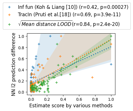
We construct our analytical model using Gaussian Processes (GPs) to model the output distribution of neural networks in response to queries on any given set of data points. We also use Neural Network Gaussian Processes (NNGPs) to reason about LOOD. NNGPs are widely used in the literature as standalone models [23], as modeling tools for different types of neural networks [18, 24, 13, 33], or as building blocks for model architecture search [25] or data distillation for generating high-utility data [19]. We empirically validate that computed LOOD under NNGP models correlates well with the performance of membership inference attacks [35, 3] against neural networks in the leave-one-out setting for benchmark datasets (Figure 3(a)). This demonstrates that our approach allows for an accurate assessment of information leakage for deep neural networks, while significantly reducing the required computation time (by more than two orders of magnitude - Footnote 4) as LOOD under NNGP can be analytically computed. As a special form of LOOD, if we measure the gap between the mean predictions of the leave-one-out models on a query, instead of quantifying the divergence between their distributions, we can estimate the influence [15, 16] and memorization (self-influence) [7, 6] metrics (Section 4.3). We experimentally show that mean distance LOOD under NNGP agrees with the actual prediction differences under leave-one-out NN retraining (Figure 3(c)), thus faithfully capturing self-influence or memorization for deep neural networks.
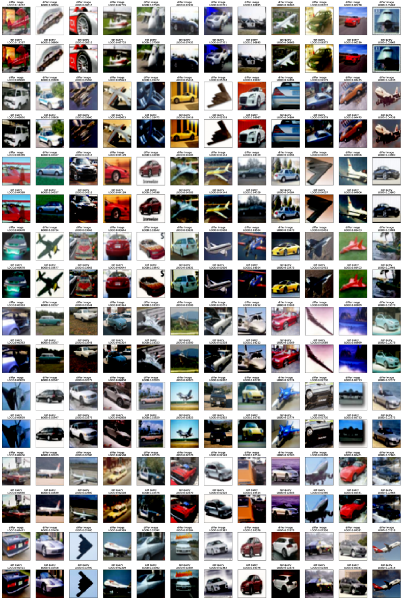
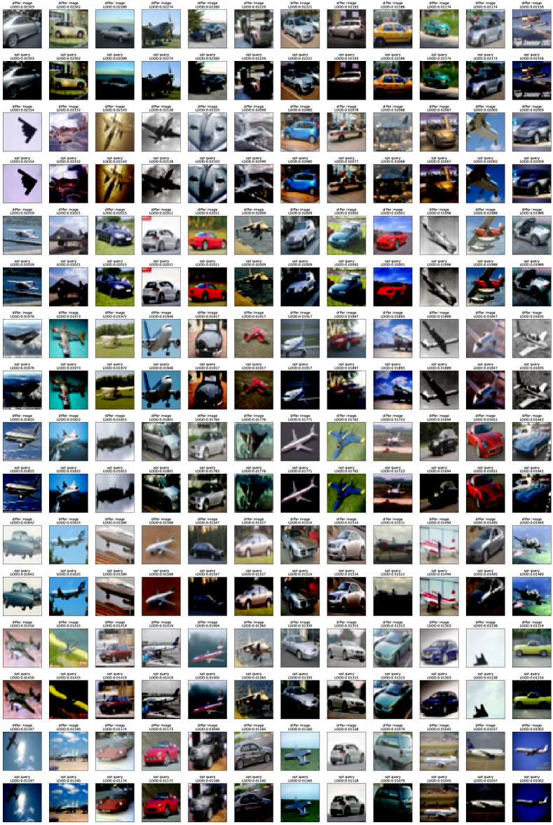
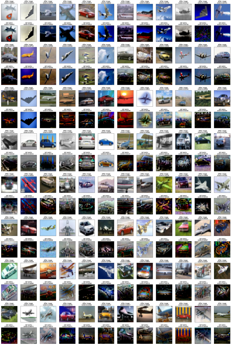
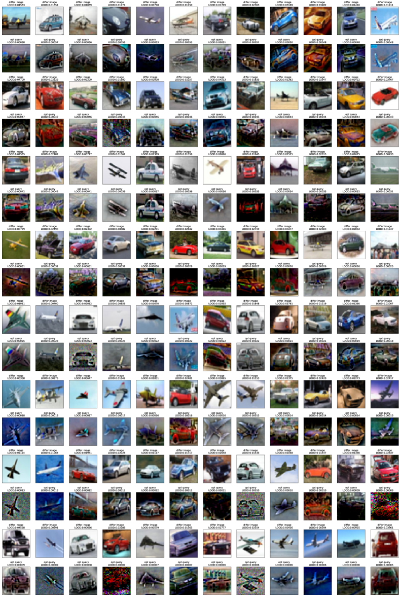
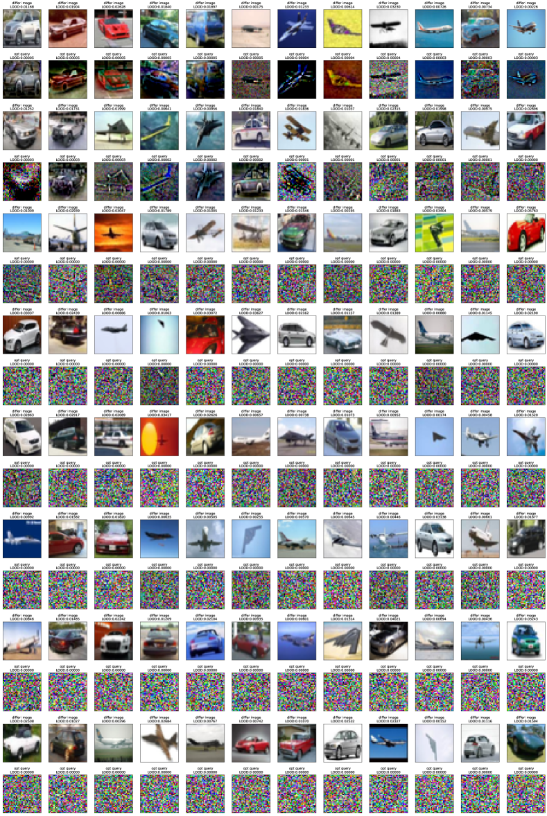
Given our framework, we prove that, for various kernel functions, including the RBF kernel and NNGP kernel on a sphere (Theorem 3.1), the differing data point itself is a stationary point of the leave-one-out distinguishability. Through experiments we further show that on image datasets, LOOD under NNGP model is maximized when the query equals the differing datapoint (2(b)). We then experimentally show that this conclusion generalizes to deep neural networks trained via SGD, by showing that the empirical information leakage is maximized when query data is within a small perturbation of the differing data (Figure 2(c)). What is interesting is that, we empirically show that LOOD remains almost unchanged even as the number of queries increases (Section E.1). In other words, all the information related to the differing point in the leave-one-out setting is contained within the model’s prediction distribution solely on that differing point. We show how to exploit this to reconstruct training (image) data in the leave-one-out or leave-one group-out settings. We present samples of the reconstructed images (See Figure 10, and 15 through 19) which show significant resemblance to the training data, even when our optimization problem lands on sub-optimal queries.
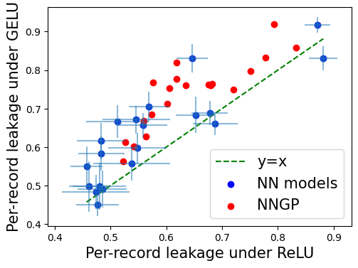
Finally, we investigate how LOOD is affected by activation functions. We prove that a low-rank kernel matrix implies low LOOD, thus low information leakage (See Proposition 5.1). Leveraging existing literature, we further show that the NNGP kernel for fully connected networks is closer to a low-rank matrix under ReLU activation (thus lead to less leakage) compared to smooth activation functions such as GeLU. We also validate this effect of activation choice result empirically, both for NNGP and for deep neural network trained via SGD (Figure 5).
2 Definition and the Analytical Framework
Definition 2.1 (Leave-one-out distinguishability).
Let and be two training datasets that differ in record(s) . Let be the distribution of model predictions given training dataset and query dataset , where the probability is taken over the randomness of the training algorithm. We define leave-one-out distinguishability as the statistical distance between and :
| (1) |
In this paper, we mainly use the KL divergence [17] as the distance function to capture the mean and covariance matrix of prediction distribution. We also use the distance between the mean predictions of and which we refer to as the Mean Distance LOOD. Different distance functions allow us to recover information leakage, memorization, and influence; see Section 4 for more details. We refer to Appendix C for a detailed discussion of why KL divergence is better suited than mean distance for measuring information leakage.
Gaussian process. To analytically capture the randomness of model outputs, without the need for empirical computation through multiple re-training, we use Gaussian Processes (GPs). A GP is specified by its mean prediction function for any input , and covariance kernel function for any pair of inputs and [32]. The mean function is typically set to e.g. zero, linear or orthogonal polynomial functions, and the covariance kernel function completely captures the structure of a Gaussian process. Some commonly used kernel functions are RBF kernels with length , and correlation kernels . The posterior prediction distribution for GP given training data (with labels ) when computed on a query data point follows the multivariate Gaussian with analytical expressions for its mean and its covariance matrix . 111This is known as Gaussian Process regression. Here for brevity, we denote by the kernel matrix given by , for and . Additionally, represents the noise in the labels: .
Neural network Gaussian process and its connections to NN training. Prior work has shown that the output of neural networks on a query converges to a Gaussian process, at initialization as the width of the NN tends to infinity [18, 29, 28]. The kernel function of the neural network Gaussian process (NNGP) is given by , where refers to the neural network weights (sampled from the prior distribution), and refers to the prediction function of the model with weights . In this case, instead of the usual gradient-based training, we can analytically compute the Gaussian Process regression posterior distribution of the network prediction given the training data and query inputs. See Appendix B for more discussions on the connections between NNGP and the training of its corresponding neural networks.
We analytically compute and analyze LOOD on NN models using the NNGP framework. We also empirically validate our theoretical results to show the NNGP-computed insights generalise to NNs.
3 Optimizing LOOD to Identify the Most Influenced Point
LOOD (1) measures the influence of training data on the prediction at record , with a higher magnitude reflecting more influence. In this section we analyse where (at which ) the model is most influenced by the change of one train datapoint . Besides shedding light on the fundamental question of influence [15] (and from there connections to adversarial robustness [8]), this question is also closely related to the open problem of constructing a worst-case query for tight privacy auditing via membership inference attacks (MIAs) [14, 21, 31, 22].
In this section, we consider a single query () and single differing point () setting and analyse the most influenced point by maximizing the LOOD:
| (2) |
both theoretically (via characterizing the landscape of the LOOD objective) and empirically (via solving problem (2) through gradient descent). Our analysis also extends generally to the multi-query () and a group of differing data () setting – see Appendix E for the details.
We first prove that for a wide class of kernel functions, the differing point is a stationary point for the LOOD maximization objective (2), i.e., satisfies the first-order optimality condition. We then validate through experimental results on image data that the differing point is the global maximum and discuss one setting where this is no longer the case.
Analysis: Differing point is a stationary point for LOOD. We first prove that if the kernel function satisfies certain regularity conditions, the gradient of LOOD at the differint point is zero, i.e., the differing data is a stationary point for LOOD (as a function of query data).
Theorem 3.1.
Let the kernel function be . Assume that (i) for all training data , i.e., all training data are normalized under kernel function ; (ii) for all training data , i.e., the kernel distance between two data records and is stable when they are equal. Then, the differing data is a stationary point for LOOD as a function of query data, as follows
The full proof of Theorem 3.1 is deferred in Section D.1. Note that Theorem 3.1 requires the kernel function to satisfy some regularity conditions. In Appendix D.2 we show the commonly used RBF kernel and NNGP kernel on a sphere satisfy these regularity conditions.
Theorem 3.1 proves that the first-order stationary condition of LOOD is satisfied when the query equals differing data. This is a necessary but not sufficient condition for maximal information leakage when query equals the differing data. However, as LOOD is a non-convex objective, it is hard to establish global optimality theoretically. Therefore, below we conduct extensive numerical experiments for Gaussian processes and deep neural networks to complement our theoretical results.
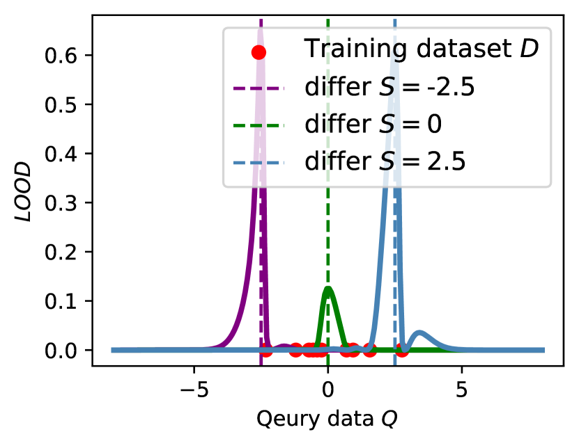
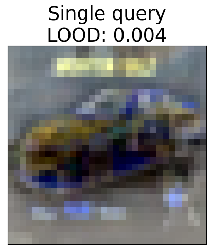
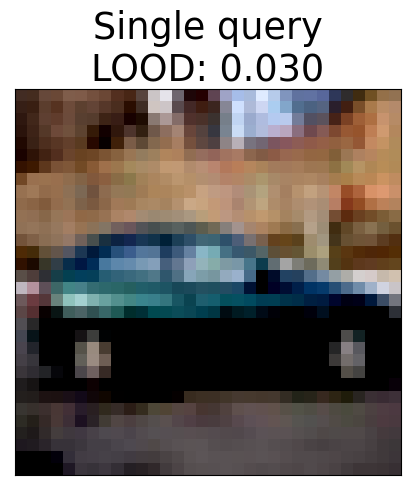
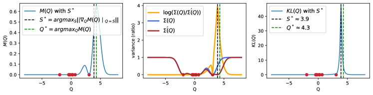
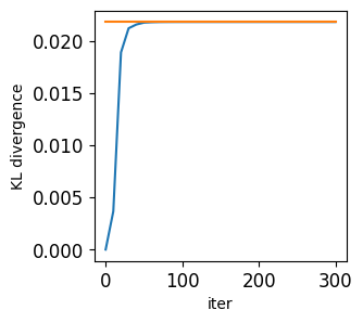
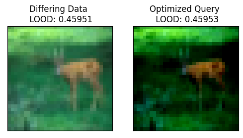
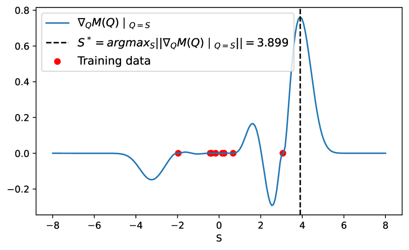
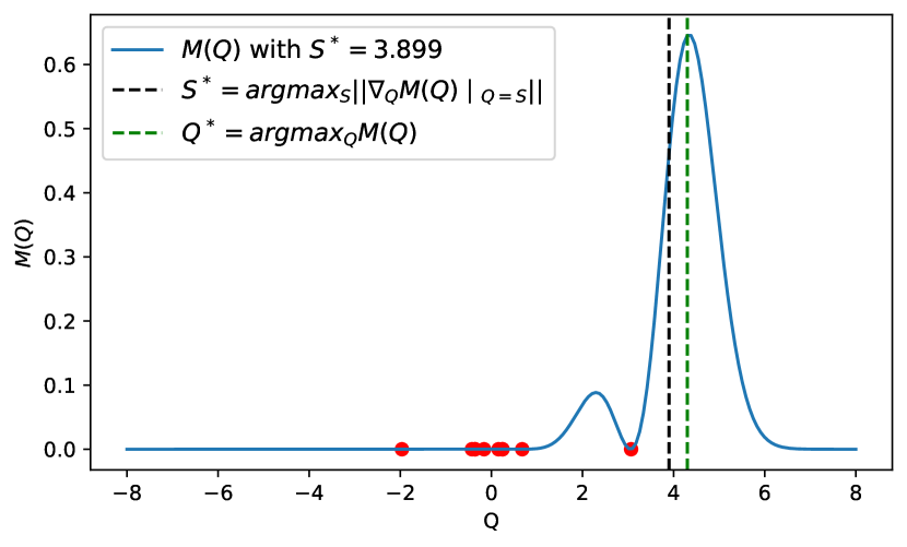
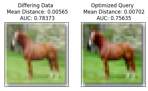
Experimental results for maximal information leakage when query equals differing data. We empirically run gradient descent on the LOOD objective (2) to find the single query that is most affected by the differing point. Figure 1 shows the optimized query under the RBF kernel. More examples of the optimized query under NNGP kernel functions are in Section D.3.
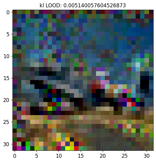
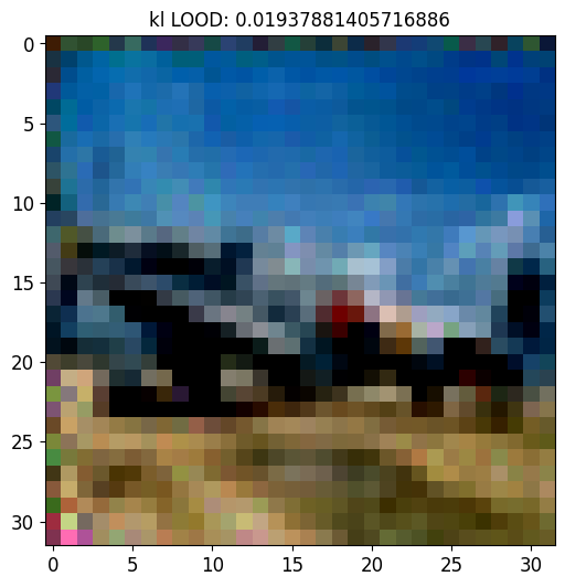
Next we present more evidence for the empirical maximality of LOOD when the query is the differing point: Figure 2(a) shows a brute-force search over the data domain of a one-dimensional toy dataset (as per the setup in Appendix D.1) to find the query with the maximal LOOD and observe that it is indeed the differing data. For the practical CIFAR10 image dataset under NNGP kernels, we examine the LOOD on queries that are perturbations of the differing data. We observe in Figure 2(b) and the caption that querying on the differing point itself consistently incurs maximal LOOD across runs with random choices of the differing data and random data perturbation directions. Finally, Figure 2(c) shows information leakage (as captured by membership inference attack performance in AUC score) of NN models on queries near the differing data for five randomly chosen differing data (this was repeated for 70 chosen differing data; see caption); we show that MIA performance is highest when query equals the differing data in 4/5 cases. 222There is one special case where the differing image is easy-to-predict and incurs low leakage on all queries. Moreover, we show that the empirical maximality of LOOD when query equals the differing data extends to the setting with multiple queries (Section E.1) and a group of differing data (Section E.2).
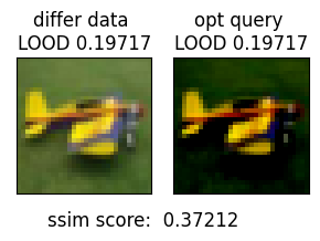
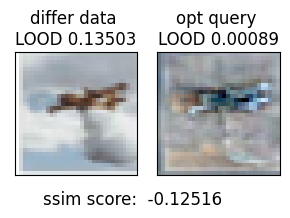
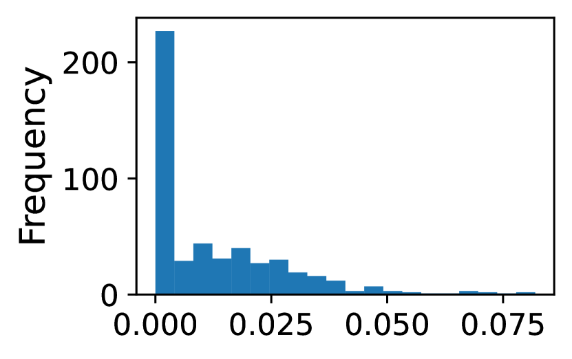
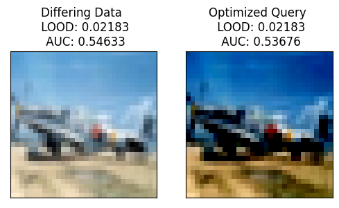
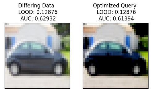
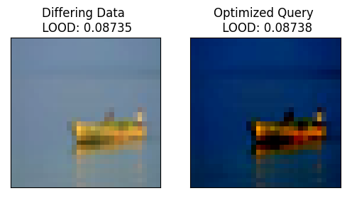
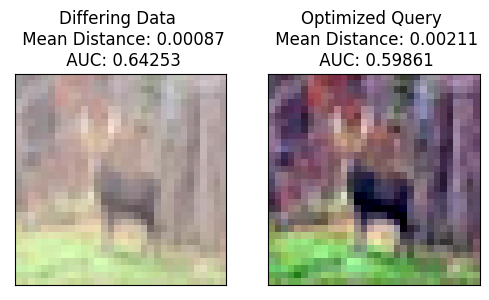
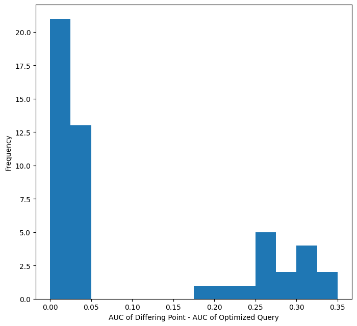
Optimized query for LOOD is close to the differing point in a majority of cases. In LOOD optimization, we observe that the optimized query could recover the differing data with high visual precision: see Figure 1(a) for an example and Figure 14-19 for more examples over randomly chosen differing data points. 333We also tried other image similarity metrics in the reconstruction attack literature, such as the per-pixel distance ([1, Section V.B] and [3, Section 5.1]), SSIM score [10, Figure 1] and LPIPS metric [1, Section V.B] – but these metrics do not reflect the visual similarity in our setting. This is possibly because the LOOD optimization objective only recovers the highest amount of information about the differing data which need not be exactly the same RGB values. LOOD optimization results in color dampening (Figure 1(a)) or color-flipped reconstruction (Figure 1(b)) of the differing data, which are not reflected by existing metrics such as SSIM score. It is a long-standing open problem to design better image similarity metrics for such reconstructions that do not preserve the exact RGB values. The optimized query also has very similar LOOD to the differing data itself consistently across random experiments, as shown in Figure 1(c). This also holds when there are more than one differing data (i.e., leave-one-group-out setting); only in one case does the optimized single query have slightly higher LOOD than the differing record that it recovers – see Figure 4 right-most column and Section E.2. We remark that, possibly due to the nonconvex structure of LOOD, cases exist where the optimized query has significantly lower LOOD than the differing data (Figure 1(b)). Noteworthy is that even in this case the query still resembles the shape of the differing data visually. As we will later show this can be leveraged for data reconstruction attacks, even for the setting where there is a group of differing data–Section 4.2 and Section E.2.
When the differing point is not the optimal query. In practice data-dependent normalization is often used prior to training. In such a setting the optimized query has a higher LOOD than the differing point itself – see Appendix D.4 for details.
4 LOOD vs. Leakage, Memorization, and Influence Measures
In this section, we show how LOOD can be applied to established definitions of information leakage based on inference attacks, influence functions, and memorization.
4.1 Quantifying Information Leakage using Leave-one-out Distinguishabilty
Information Leakage relates to the extent to which a model’s output can unintentionally reveal information about the training dataset when the model’s prediction (distribution) at a query is observed by an adversary. One established method for assessing it is through a membership inference attack (MIA) [30], where an attacker attempts to guess whether a specific data point was part of the model’s training dataset; the leakage is quantified by the attacker’s false positive rate (FPR) versus his true positive rate (TPR), as well as the the area under the TPR-FPR curve (AUC), when performed on randomly trained target models and its training/test data records. However, performing computing the leakage using MIA can be computationally expensive due to the associated costs of retraining many models on a fixed pair of leave-one-out datasets. Using LOOD with Gaussian processes is an efficient alternative that allows to answer: i) Which query should the attacker use to extract the highest possible amount of information leakage regarding ? (Section 3), and ii) How much is a specific record at risk based on its worst-case query, effectively quantifying the information leakage associated with each training record.
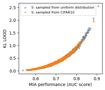
LOOD demonstrates information leakage in NNGP. We first investigate whether the LOOD when querying the differing record itself accurately reflects the level of information leakage in a membership inference attack. For an MIA to successfully distinguish between two prediction distributions of models trained on leave-one-out datasets and with the differing record , it must be able to effectively differentiate between and . Intuitively, the success of MIA (as measured by its AUC score) implies a high distinguishability between these two distributions. In Figure 3(b), we observe a strong correlation between LOOD and the performance of MIA. This finding leads us to conclude that LOOD effectively reflects information leakage in NNGP predictions.
NNGP effectively and efficiently captures leakage under practical neural network training. In Section 3, we establish the theoretical first-order stationary condition, and empirical optimality of LOOD (information leakage) when the query is the differing data point. In this section, we further explore whether the leakage computed using NNGP models accurately reflects the leakage empirically measured in neural network models which are trained using SGD. To measure leakage, we utilize the success of the membership inference attacks (AUC score) when observing predictions from NN models trained on leave-one-out datasets. In Figure 3(a), we compare the MIA performance between NNGP models and neural network models. Notably, we observe a strong correlation, suggesting that NNGP captures the information leakage of neural networks about training data records.
One significant advantage of using NNGPs to estimate leakage is the efficiency of analytic expressions, which significantly reduces computational requirements. In the analysis of Figure 3(a), we observed over speed up for estimating leakage using our framework versus empirically measuring it as it is performed in the literature [2, 35].444Lauching the empirical MIA in Figure 3(a) involved training FC networks, which took approximately GPU hours. For the same setting, obtaining the LOOD results only required around GPU minutes.
4.2 Optimizing LOOD as a Data Reconstruction Attack
A strong threat against machine learning models is an adversary that reconstructs the data points with significant (MIA) likelihood of being in the training set [3]. In Figure 1 and Figure 14-19, we have demonstrated that optimizing LOOD for a query often leads to the recovery of the differing data point. This is due to the significant amount of information that is being leaked through the model’s prediction on the differing data itself. Such results showcase that LOOD can be leveraged for a data reconstruction attack in a setting where the adversary has access to at least part of the train data. Notably, the prior works of [1, 9] focus on reconstruction attacks under the assumption that the adversary possesses knowledge of all data points except for one (which aligns with our leave-one-out setting).
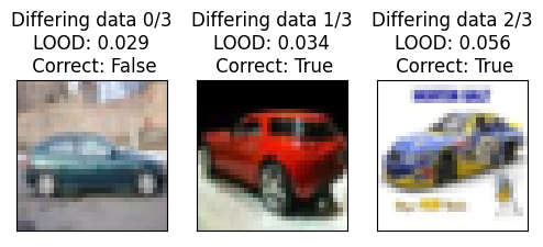
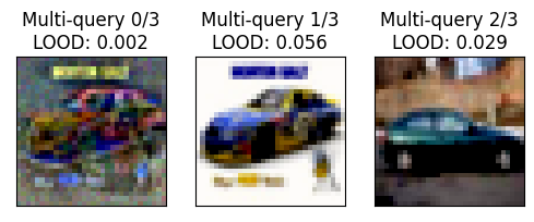 |
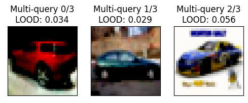 |
 |
 |
Our reconstruction via optimizing LOOD methodology also extends to the group setting. In Figure 4, we present results demonstrating that even when the attacker does not know a group of data points and has access to the model distribution on the complete dataset, they can successfully reconstruct the whole group of differing data points with a high degree of visual similarity. Additionally, by examining the frequency of LOOD optimization converging to a query close to each data point in the differing group (across multiple runs and optimized queries), we can assess which ’s are most vulnerable to reconstruction – see Section E.2 for more details. Reconstruction under the leave-one-group-out setting mimics a more practical real world adversary that aims to reconstruct more than one training data. In the limit of large group size that equals the size of the training dataset, such leave-one-group-out setting recovers one of the difficult reconstruction attack scenario studied in [10], where the adversary does not have exact knowledge about any training data. Therefore, extending our results within the leave-one-group-out setting to practical reconstruction attacks presents a promising open problem for future exploration.
4.3 Analysis of Influence and Memorization
Influence functions [27, 16, 15] quantify the degree of change in the model’s prediction (error) for a record when a data record is added to the training dataset . A closely related concept is memorization [6, 7], which can be modeled as self-influence. In terms of definitions, certain prior influence [15] and memorization (i.e., self-influence) [6, 7] definitions can be recovered as special cases of LOOD if we measure the distance between the mean predictions of the leave-one-out models on a query, instead of quantifying the divergence between their distributions. We discuss the detailed relations between the concepts in Appendix F.
Mean distance LOOD under NNGP agrees with leave-one-out NN retraining. In Figure 3(c), we show that mean distance LOOD agrees with the actual prediction differences under leave-one-out retraining. In the -axis, we show the actual prediction difference between 100 NN models trained on each of the leave-one-out datasets, over 50 randomly chosen differing data. This is exactly the memorization or self-influence as defined by [6, Page 5] and [7, Equation 1], and serves as a ground-truth baseline that should be matched by good influence estimations. In the -axis, we show the normalized mean distance LOOD (under NNGP), influence function [15] and TracIn estimates [26]. We observe that mean distance LOOD has the highest correlation to the actual prediction difference among all methods.
Analysis of Influence and memorization via mean distance LOOD. LOOD can thus be seen as a generalization of the prior metrics that allows to account for higher-order differences in the distributions. Measuring influence and memorization using our framework offers a computationally efficient methodology, and thus allows us to answer questions such as: Where, i.e., at which query , does the model exhibit the most influence? Which data record has the largest influence? How do different model architectures impact influence? Answers to these questions can be derived in a similar manner as the analysis for LOOD that we provide in other parts (Section 3 and Section 5) of the paper. As a concrete example, we show how to use mean distance LOOD for a more fine-grained assessment of influence within our analytical framework. Proposition 4.1 provides valuable insights into influence analysis using the different behaviors of Mean LOOD, based on where the differing point is located with respect to the rest of the training set. This allows us to answer the question: Which data record has the most significant influence and at which query ?
Proposition 4.1 (First-order optimality condition for influence).
Consider a dataset , a differing point , and a kernel function satisfying the same conditions of Theorem 3.1. Then, we have that
where is the mean distance LOOD in C.1, are kernel matrices as defined in Section 2, , , and .
Our first observation from Proposition 4.1 is that when is far from the dataset in the sense that , the mean distance LOOD gradient is close to , i.e., the differing data is a stationary point for the mean distance LOOD objective. We also analyze the second-order Hessian condition of mean distance LOOD in Lemma G.4, and prove that the differing data has locally maximal influence, as long as far from the remaining training dataset , and the data labels are bounded (which is the case in a classification task). In the opposite case where is close to in the sense that (i.e., is perfectly predicted by the GP trained on remaining dataset ), then the gradient of mean distance LOOD is also close to zero.
Between the above two cases, when the differing data is neither too close nor too far from the remaining dataset, Proposition 4.1 proves that in general , i.e., the differing data is not optimal for the mean distance LOOD maximization objective Equation 2. To give an intuition, we can think of the Mean LOOD as the result of an interaction of two forces, a force due to the training points, and another force due to the differing point. When the differing point is neither too far nor too close to the training data, the synergy of the two forces creates a region that does not include the differing point where the LOOD is maximal. To further illustrate these patterns and optimality region of mean distance LOOD, we provide numerical examples for RBF kernel on toy dataset in Figures 11(b)-12, and for NNGPs on image data in Figures 13(a)-13(c) in Appendix G.
5 Explaining the Effect of Activation Functions on LOOD
In this section, we theoretically investigate the effect of activation function on the magnitude of LOOD (given fixed leave-one-out datasets). We will leverage Footnote 8 in the Appendix; it shows that for the same depth, smooth activations such that GeLU are associated with kernels that are farther away from a low rank all-constant matrix (more expressive) than kernel obtained with non-smooth activations, e.g. ReLU. To understand the effect of activation, we only need to analyze how the low-rank property of NNGP kernel matrix affects the magnitude of LOOD (leakage), given a fixed pair of differing point and remaining dataset . To this end, we establish the following proposition, which shows that the LOOD (leakage) is small if the NNGP kernel matrix for the training dataset is close to a low rank all-constant matrix.
Proposition 5.1 (Informal: Low rank kernel matrix implies low LOOD).
Let and be an arbitrary pair of leave-one-out datasets, where contains records and contains records. Define the function . Let , and thus quantifies how close the kernel matrix is to a low rank all-constant matrix. Assume that . Then, there exist constants such that
Thus LOOD should decrease as decreases, see Proposition H.1 for formal statement and proofs.
Proposition 5.1 proves that the LOOD is upper bounded by the term that captures how close the kernel matrix is to an all-constant matrix (of low rank one), thus implying smaller LOOD (leakage) over worst-case query given low rank kernels. Intuitively, this happens because the network output forgets most of the information about the input dataset under low rank kernel matrix.
Analysis: smooth activation functions induce higher LOOD (leakage). We have shown that low rank kernels are associated with smaller LOOD (leakage) over worst-case query (Proposition 5.1) and NNGP kernel converges to a constant kernel at different rates under different activations (Footnote 8 and [29, 11, 12]). By combining them we conclude that LOOD (leakage) is higher under smooth activations (such as GeLU) than non-smooth activations (such as ReLU). This is consistent with the intuition that smooth activations allow deeper information propagation, thus inducing more expressive kernels and more memorization of the training data. Interestingly, recent work [4] also showed that GeLU enables better model performance than ReLU even in modern architectures such as ViT. Our results thus suggest there is a privacy-accuracy tradeoffs by activation choices.
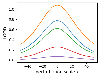
Empirical results: NNGP with GeLU activation induces higher LOOD than ReLU activation. We now empirically investigate how the activation function affects the LOOD under NNGP. Our experiment setting is NNGP for fully connected neural networks with varying depth . The training dataset contains ’plane’ and ’car’ images from CIFAR10. We evaluted LOOD over randomly chosen differing data, and observe under fixed depth, the computed LOOD under ReLU is more than higher than LOOD under GeLU in cases. We visualize randomly chosen differing data in Figure 5. Under each fixed differing data, we also observe that the gap between LOOD under ReLU and LOOD under GeLU grows with the depth. This is consistent with the pattern predicted by our analysis in Footnote 8, i.e., GeLU gives rise to higher leakage in LOOD than ReLU activation, and their gap increases with depth. It is worth noting that for our experiments the LOOD optimization is done without constraining the query data norm. Therefore, our experiments shows that the result of Footnote 8 could be valid in more general settings.
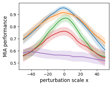
Effect of activation function on LOOD generalizes to information leakage on NN models. We further investigate whether the information leakage (as measured by membership inference attack performance for leave-one-out retrained models) for deep neural networks are similarly affected by activation function. Figure 5 shows that deep nerual networks with GeLU activation incurs higher per-record information leakage (MIA performance in AUC score) compared to NNs with ReLU activation, for randomly chosen differing data. This is consistent with our analytical results (Footnote 8 and 5.1) that predict higher LOOD under smooth activation than under ReLU.
6 Conclusions
We have presented a formal framework using Gaussian processes to quantify the influence of individual training data points on predictions of machine learning models. We also explore the collective influence of groups of data points and their potential risk with respect to inference attacks. Our work sheds light on the privacy implications of model predictions on training data, and generalizes the work on influence analysis and memorization.
References
- Balle et al. [2022] Borja Balle, Giovanni Cherubin, and Jamie Hayes. Reconstructing training data with informed adversaries. In 2022 IEEE Symposium on Security and Privacy (SP), pages 1138–1156. IEEE, 2022.
- Carlini et al. [2022] Nicholas Carlini, Steve Chien, Milad Nasr, Shuang Song, Andreas Terzis, and Florian Tramer. Membership inference attacks from first principles. In 2022 IEEE Symposium on Security and Privacy (SP), pages 1897–1914. IEEE, 2022.
- Carlini et al. [2023] Nicholas Carlini, Jamie Hayes, Milad Nasr, Matthew Jagielski, Vikash Sehwag, Florian Tramer, Borja Balle, Daphne Ippolito, and Eric Wallace. Extracting training data from diffusion models. arXiv preprint arXiv:2301.13188, 2023.
- Dosovitskiy et al. [2021] Alexey Dosovitskiy, Lucas Beyer, Alexander Kolesnikov, Dirk Weissenborn, Xiaohua Zhai, Thomas Unterthiner, Mostafa Dehghani, Matthias Minderer, Georg Heigold, Sylvain Gelly, Jakob Uszkoreit, and Neil Houlsby. An image is worth 16x16 words: Transformers for image recognition at scale. In International Conference on Learning Representations, 2021.
- Dwork et al. [2014] Cynthia Dwork, Aaron Roth, et al. The algorithmic foundations of differential privacy. Found. Trends Theor. Comput. Sci., 9(3-4):211–407, 2014.
- Feldman [2020] Vitaly Feldman. Does learning require memorization? a short tale about a long tail. In Proceedings of the 52nd Annual ACM SIGACT Symposium on Theory of Computing, pages 954–959, 2020.
- Feldman and Zhang [2020] Vitaly Feldman and Chiyuan Zhang. What neural networks memorize and why: Discovering the long tail via influence estimation. Advances in Neural Information Processing Systems, 33:2881–2891, 2020.
- Goodfellow et al. [2014] Ian J Goodfellow, Jonathon Shlens, and Christian Szegedy. Explaining and harnessing adversarial examples. arXiv preprint arXiv:1412.6572, 2014.
- Guo et al. [2022] Chuan Guo, Brian Karrer, Kamalika Chaudhuri, and Laurens van der Maaten. Bounding training data reconstruction in private (deep) learning. In International Conference on Machine Learning, pages 8056–8071. PMLR, 2022.
- Haim et al. [2022] Niv Haim, Gal Vardi, Gilad Yehudai, Ohad Shamir, and Michal Irani. Reconstructing training data from trained neural networks. arXiv preprint arXiv:2206.07758, 2022.
- Hayou et al. [2019] Soufiane Hayou, Arnaud Doucet, and Judith Rousseau. On the impact of the activation function on deep neural networks training. In International Conference on Machine Learning, 2019.
- Hayou et al. [2021] Soufiane Hayou, Eugenio Clerico, Bobby He, George Deligiannidis, Arnaud Doucet, and Judith Rousseau. Stable resnet. In Arindam Banerjee and Kenji Fukumizu, editors, Proceedings of The 24th International Conference on Artificial Intelligence and Statistics, volume 130 of Proceedings of Machine Learning Research, pages 1324–1332. PMLR, 13–15 Apr 2021.
- Hron et al. [2020] Jiri Hron, Yasaman Bahri, Jascha Sohl-Dickstein, and Roman Novak. Infinite attention: Nngp and ntk for deep attention networks. In International Conference on Machine Learning, pages 4376–4386. PMLR, 2020.
- Jagielski et al. [2020] Matthew Jagielski, Jonathan Ullman, and Alina Oprea. Auditing differentially private machine learning: How private is private sgd? Advances in Neural Information Processing Systems, 33:22205–22216, 2020.
- Koh and Liang [2017] Pang Wei Koh and Percy Liang. Understanding black-box predictions via influence functions. In International conference on machine learning, pages 1885–1894. PMLR, 2017.
- Koh et al. [2019] Pang Wei W Koh, Kai-Siang Ang, Hubert Teo, and Percy S Liang. On the accuracy of influence functions for measuring group effects. Advances in neural information processing systems, 32, 2019.
- Kullback and Leibler [1951] Solomon Kullback and Richard A Leibler. On information and sufficiency. The annals of mathematical statistics, 22(1):79–86, 1951.
- Lee et al. [2017] Jaehoon Lee, Yasaman Bahri, Roman Novak, Samuel S Schoenholz, Jeffrey Pennington, and Jascha Sohl-Dickstein. Deep neural networks as gaussian processes. arXiv preprint arXiv:1711.00165, 2017.
- Loo et al. [2022] Noel Loo, Ramin Hasani, Alexander Amini, and Daniela Rus. Efficient dataset distillation using random feature approximation. arXiv preprint arXiv:2210.12067, 2022.
- Lou et al. [2022] Yizhang Lou, Chris E Mingard, and Soufiane Hayou. Feature learning and signal propagation in deep neural networks. In International Conference on Machine Learning, pages 14248–14282. PMLR, 2022.
- Nasr et al. [2021] Milad Nasr, Shuang Songi, Abhradeep Thakurta, Nicolas Papernot, and Nicholas Carlin. Adversary instantiation: Lower bounds for differentially private machine learning. In 2021 IEEE Symposium on Security and Privacy (SP), pages 866–882. IEEE, 2021.
- Nasr et al. [2023] Milad Nasr, Jamie Hayes, Thomas Steinke, Borja Balle, Florian Tramèr, Matthew Jagielski, Nicholas Carlini, and Andreas Terzis. Tight auditing of differentially private machine learning. arXiv preprint arXiv:2302.07956, 2023.
- Neal [2012] Radford M Neal. Bayesian learning for neural networks, volume 118. Springer Science & Business Media, 2012.
- Novak et al. [2018] Roman Novak, Lechao Xiao, Jaehoon Lee, Yasaman Bahri, Greg Yang, Jiri Hron, Daniel A Abolafia, Jeffrey Pennington, and Jascha Sohl-Dickstein. Bayesian deep convolutional networks with many channels are gaussian processes. arXiv preprint arXiv:1810.05148, 2018.
- Park et al. [2020] Daniel S. Park, Jaehoon Lee, Daiyi Peng, Yuan Cao, and Jascha Sohl-Dickstein. Towards nngp-guided neural architecture search, 2020.
- Pruthi et al. [2020] Garima Pruthi, Frederick Liu, Satyen Kale, and Mukund Sundararajan. Estimating training data influence by tracing gradient descent. Advances in Neural Information Processing Systems, 33:19920–19930, 2020.
- Rousseeuw et al. [2011] Peter J Rousseeuw, Frank R Hampel, Elvezio M Ronchetti, and Werner A Stahel. Robust statistics: the approach based on influence functions. John Wiley & Sons, 2011.
- Schoenholz et al. [2016] Samuel S Schoenholz, Justin Gilmer, Surya Ganguli, and Jascha Sohl-Dickstein. Deep information propagation. arXiv preprint arXiv:1611.01232, 2016.
- Schoenholz et al. [2017] S.S. Schoenholz, J. Gilmer, S. Ganguli, and J. Sohl-Dickstein. Deep information propagation. In International Conference on Learning Representations, 2017.
- Shokri et al. [2017] Reza Shokri, Marco Stronati, Congzheng Song, and Vitaly Shmatikov. Membership inference attacks against machine learning models. In 2017 IEEE symposium on security and privacy (SP), pages 3–18. IEEE, 2017.
- Wen et al. [2022] Yuxin Wen, Arpit Bansal, Hamid Kazemi, Eitan Borgnia, Micah Goldblum, Jonas Geiping, and Tom Goldstein. Canary in a coalmine: Better membership inference with ensembled adversarial queries. arXiv preprint arXiv:2210.10750, 2022.
- Williams and Rasmussen [2006] Christopher KI Williams and Carl Edward Rasmussen. Gaussian processes for machine learning. MIT press Cambridge, MA, 2006.
- Yang [2019] Greg Yang. Wide feedforward or recurrent neural networks of any architecture are gaussian processes. Advances in Neural Information Processing Systems, 32, 2019.
- Yang and Littwin [2023] Greg Yang and Etai Littwin. Tensor programs ivb: Adaptive optimization in the infinite-width limit. arXiv preprint arXiv:2308.01814, 2023.
- Ye et al. [2022] Jiayuan Ye, Aadyaa Maddi, Sasi Kumar Murakonda, Vincent Bindschaedler, and Reza Shokri. Enhanced membership inference attacks against machine learning models. In Proceedings of the 2022 ACM SIGSAC Conference on Computer and Communications Security, pages 3093–3106, 2022.
Appendix A Table of Notations
| Symbol | Meaning | |||
|---|---|---|---|---|
| Leave-one-out dataset | ||||
| Leave-one-out dataset combined with the differing data | ||||
| Differing data record(s) | ||||
| number of differing data records | ||||
| Queried data record (s) | ||||
| number of queries | ||||
| dimension of the data | ||||
| Kernel function | ||||
|
||||
| Abbreviation for | ||||
| Abbreviation for | ||||
| Abbreviation for | ||||
|
||||
| MIA | Abbreviation for membership inference attack |
Appendix B Additional discussion on the connections between NNGP and NN training
Note that in general, there is a performance gap between a trained NN and its equivalent NNGP model. However, they are fundamentally connected even when there is a performance gap: the NNGP describes the (geometric) information flow in a randomly initialized NN and therefore captures the early training stages of SGD-trained NNs. In a highly non-convex problem such as NN training, the initialization is crucial and its impact on different quantities (including performance) is well-documented [28]. Moreover, it is also well-known that the bulk of feature learning occurs during the first few epochs of training (see [20, Figure 2]), which makes the initial training stages even more crucial. Hence, it should be expected that properties of NNGP transfer (at least partially) to trained NNs. More advanced tools such as Tensor Programs [34] try to capture the covariance kernel during training, but such dynamics are generally intractable in closed-form.
Appendix C Deferred details for Section 2
C.1 Mean Distance LOOD
The simplest way of quantifying the LOOD is by using the distance between the means of the two distributions formed by coupled Gaussian processes:
Definition C.1 (Mean distance LOOD).
By computing the distance between the mean of coupled Gaussian processes on query set , we obtain the following mean distance LOOD.
| (3) | ||||
| (4) |
where is a query data record, and and are the mean of the prediction function for GP trained on and respectively, as defined in Section 2. When the context is clear, we abbreviate and in the notation and use under differing data to denote where .
Example C.2 (Mean distance LOOD is not well-correlated with MIA success).
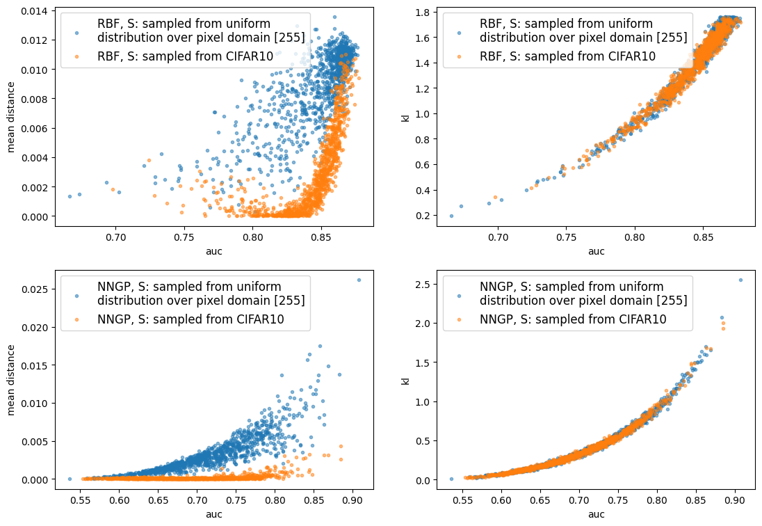
We show the correlations between Mean distance LOOD and the success of leave-one-out membership inference attack (MIA) 555This is measured by the AUC of the attacker’s false positive rate (FPR) versus his true positive rate (TPR). in Figure 6 (left). We observe that low mean distance and high AUC score occur at the same time, i.e., low Mean distance LOOD does not imply low attack success. This occurs especially when the differing point is sampled from a uniform distribution over the pixel domain .
Another downside of the mean distance LOOD metric is that solely first-order information is incorporated; this results in it being additive in the queries: . That is, Mean distance LOOD does not allow to incorporate the impact of correlations between multiple queries. Moreover, the mean distance LOOD has a less clear interpretation under certain kernel functions. For example, under the NNGP kernel, a query with large norm will also have high Mean Distance LOOD (despite normalized query being the same), due to the homogeneity of NNGP kernel. By contrast, as we show below, KL divergence (relative entropy) LOOD mitigates these limitations.
C.2 KL Divergence LOOD
To mitigate the downsides of Mean distance LOOD and incorporate higher-order information, we use KL divergence (relative entropy) LOOD.
Definition C.3 (KL Divergence LOOD).
Let be the set of queried data points, where is the data feature dimension and is the number of queries. Let be a pair of leave-one-out datasets such that where is the differing data point. Let and as coupled Gaussian processes given and . Then the Leave-one-out KL distinguishability between and on queries is as follows,
| (5) | ||||
| (6) |
where for brevity, we denote , , , and as defined in Section 2.
Example C.4 (KL divergence is better correlated with MIA success).
We show correlations between KL Divergence LOOD and AUC score of the MIA in Figure 6 (right). We observe that KL Divergence LOOD and AUC score are well-correlated with each other.
On the assymmetry of KL divergence. In this paper we restrict our discussions to the case when the base distribution in KL divergence is specified by the predictions on the larger dataset , which is a reasonable upper bound on the KL divergence with base distribution specified by predictions on the smaller dataset. This is due to the following observations:
-
1.
In numerical experiments (e.g., the middle figure in Figure 7) that across varying single query . This is aligned with the intuition that the added information in the larger dataset reduce its prediction uncertainty (variance).
-
2.
If , then we have that
Proof.
Denote , then by Equation 6, for single query , we have that
(7) where is the abbreviation for mean distance LOOD as defined in Definition C.1. Similarly, when the base distribution of KL divergence changes, we have that
(8) Therefore, we have that
For , we have that and . Therefore, we have that as long as . ∎
Therefore, the KL divergence with base prediction distribution specified by the larger dataset is an upper bound for the worst-case KL divergence between prediction distributions on leave-one-out datasets.
C.3 Comparison between Mean Distance LOOD and KL Divergence LOOD
KL Divergence LOOD is better correlated with attack performance. As observed from Figure 6, KL divergence LOOD exhibits strong correlation to attack performances in terms of AUC score of the corresponding leave-one-out MIA. By contrast, Mean distance LOOD is not well-correlated with MIA AUC score. For example, there exist points that incur small mean distance LOOD while exhibiting high privacy risk in terms of AUC score under leave-one-out MIA. Moreover, from Figure 6 (right), empirically there exists a general threshold of KL Divergence LOOD that implies small AUC (that persists under different choices of kernel function, and dataset distribution). This is reasonable since KL divergence is the mean of negative log-likelihood ratio, and is thus closely related to the power of log-likelihood ratio membership inference attack.
Why the mean is (not) informative for leakage. To understand when and why there are discrepancies between the mean distance LOOD and KL LOOD, we numerically investigate the optimal query that incurs maximal mean distance LOOD. In Figure 7, we observe that although indeed incurs the largest mean distance among all possible query data, the ratio between prediction variance of GP trained on and that of GP trained on , is also significantly smaller at query when compared to the differing point . Consequently, after incorporating the second-order variance information, the KL divergence at query is significantly lower than the KL divergence at the differing point , despite of the fact that incurs maximal mean distance LOOD. A closer look at Figure 7 middle indicates that the variance ratio peaks at the differing point , and drops rapidly as the query becomes farther away from the differing data and the training dataset. Intuitively, this is because , i.e., the variance at the larger dataset, is extremely small at the differing data point . As the query gets further away from the larger training dataset, then increases rapidly. By contrast, the variance on the smaller dataset is large at the differing data point , but does not change a lot around its neighborhood, thus contributing to low variance ratio. This shows that there exist settings where the second order information contributes significantly to the information leakage, which is not captured by mean distance LOOD (as it only incorporates first-order information).
As another example case of when the variance of prediction distribution is non-negligible for faithfully capturing information leakage, we investigate under kernel functions that are homogeneous with regard to their input data. Specifically, for a homogeneous kernel function that satisfifes for any real number , we have that
where denotes the variance of the label noise. Therefore, for any , we have that
| (9) | ||||
| (10) |
Consequently, the query that maximizes Mean distance LOOD explodes to infinity for data with unbounded domain. On the contrary, the KL Divergence LOOD is scale-invariant and remains stable as the query scales linearly (because it takes the variance into account, which also grows with the query scale). In this case, the mean distance is not indicative of the actual information leakage as the variance is not a constant and is non-negligible.
In summary, KL LOOD is a metric that is better-suited for the purpose of measuring information leakage, compared to mean distance LOOD. This is because KL LOOD captures the correlation between multiple queries, and incorporates the second-order information of prediction distribution.
Appendix D Deferred proofs and experiments for Section 3
D.1 Deferred proof for Theorem 3.1
In this section, we prove that the differing data record is the stationary point for optimizing the LOOD objective. We will need the following lemma.
Lemma D.1.
For , and , we have that
| (11) |
where .
We now proceed to prove Theorem 3.1
Theorem 3.1.
Let the kernel function be . Assume that (i) for all training data , i.e., all training data are normalized under kernel function ; (ii) for all training data , i.e., the kernel distance between two data records and is stable when they are equal. Then, the differing data is a stationary point for LOOD as a function of query data, as follows
Proof.
In this statement, LOOD refers to KL LOOD Definition C.3, therefore by analytical differentiation of Definition C.3, we have that
| (12) | ||||
| (13) |
Note that here and are both scalars, as we consider single query. We denote the three terms by , , and . We will show that and which is sufficient to conclude. Let us start with the first term.
-
1.
: Recall from the Gaussian process definition in Section 2 that
where . Therefore,
where ( is the dimension of and is the number of datapoints in the training set ). A similar formula holds for .
From Lemma D.1, and by using the kernel assumption that , we have that
(14) (15) where .
Using the fact that where , simple calculations yield
We now have all the ingredients for the first term. To alleviate the notation, we denote by .
We obtain
A key observation here is the fact that the last entry of is by assumption. Using the formula above for , we obtain
Now observe that , which concludes the proof for the first term.
-
2.
:
Let us start by simplifying . The derivative here is that of , and we have
Using the formula of and observe that the last entry of is zero, we obtain
Moreover, we have that
(16) (17) (18) (19) (20) Therefore
(21) Let us now deal with . We have that
(22) By plugging Equation 22 and 20 into , we prove that
We conclude by observing that .
∎
D.2 Proofs for regularity conditions of commonly used kernel functions
We first show that both the isotropic kernel and the correlation kernel satisfies the condition of Theorem 3.1. We then show that the RBF kernel, resp. the NNGP kernel on a sphere, is an isotropic kernel, resp. a correlation kernel.
Proposition D.2 (Isotropic kernels satisfy conditions in Theorem 3.1).
Assume that the kernel function is isotropic, i.e. there exists a continuously differentiable function such that for all . Assume that satisfies is bounded666Actually, only the boundedness near zero is needed. and . Then, satisfies the conditions of Theorem 3.1.
Proof.
It is straightforward that for all . Simple calculations yield
By assumption, the term is bounded for all and also in the limit . Therefore, it is easy to see that
More rigorously, the partial derivative above exists by continuation of the function near . ∎
Proposition D.3 (Correlation kernels satisfy conditions in Theorem 3.1).
Assume that the kernel function is a correlation kernel, i.e. there exists a function such that for all . Assume that . Then, satisfies the conditions of Theorem 3.1.
Proof.
The first condition is satisfied by assumption on . For the second condition, observe that
which yields . ∎
We have the following result for the NNGP kernel.
Proposition D.4 (NNGP kernel on the sphere satisfies conditions in Theorem Theorem 3.1).
The NNGP kernel function is similar to the correlation kernel. For ReLU activation function, it has the form
This kernel function does not satisfy the conditions of Theorem 3.1 and therefore we cannot conclude that the differing point is a stationary point. Besides, in practice, NNGP is used with normalized data in order to avoid any numerical issues; the datapoints are normalized to have for some fixed . With this formulation, we can actually show that the kernel restricted to the sphere satisfies the conditions of Theorem 3.1. However, as one might guess, it is not straightforward to compute a "derivative on the sphere" as this requires a generalized definition of the derivative on manifolds (the coordinates are not free). To avoid dealing with unnecessary complications, we can bypass this problem by considering the spherical coordinates instead. For , there exists a unique set of parameters s.t.
This is a generalization of the polar coordinates in .
Without loss of generality, let us assume that and let . In this case, the NNGP kernel, evaluated at is given by
with the convention .
Consider the spherical coordinates introduced above, and assume that . Then, the NNGP kernel given by satisfies the conditions of Theorem 3.1.
Proof.
Computing the derivative with respect to is equivalent to computing the derivative on the unit sphere. For , we have
where
When , we obtain
By observing that
we conclude that for all .
∎
D.3 More examples for query optimization under NNGP kernel functions
We show the optimized query for NNGP kernel under different model architectures, including fully connected network and convolutional neural network with various depth, in Figure 8.
To further understand the query optimization process in details, we visualize an example LOOD optimization process below in Figure 9.
D.4 When the differing point is not the optimal query
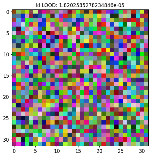
In practice data-dependent normalization is used prior to training, such as batch and layer normalization. Note that this normalization of the pair of leave-one-out datasets results in them differing in more than one record 777During inference, the same test record will again go through a normalization step that depends on the training dataset before being passed as a query the corresponding Gaussian process. Then the optimised query data record obtains a higher LOOD than the LOOD of the differing points; we show this in Figure 10; thus in such a setting there is value for the attacker to optimise the query; this is consistent with results from [31] that exploit the training data augmentation.
Appendix E Analyzing LOOD for Multiple Queries and Leave-one-group-out Setting
E.1 LOOD under multiple queries
We now turn to a more general question of quantifying the LOOD when having a model answer multiple queries rather than just one query (this corresponds to the practical setting of e.g. having API access to a model that one can query multiple times). In this setting, a natural question is: as the number of queries grows, does the distinguishability between leave-one-out models’ predictions get stronger (when compared to the single query setting)? Our empirical observations indicate that the significant information regarding the differing data point resides within its prediction on that data record. Notably, the optimal single query exhibits a higher or equal degree of leakage compared to any other query set.
Specifically, to show that the optimal single query exhibits a higher or equal degree of leakage compared to any other query set, we performed multi-query optimization , which uses gradient descent to optimize the LOOD across queries, for varying numbers of queries . We evaluated this setting under the following conditions: NNGP using a fully connected network with depths of ; using random selections of leave-one-out datasets (where the larger dataset is of size ) sampled from the ’car’ and ’plane’ classes of the CIFAR10 dataset. Our observations indicate that, in all evaluation trials, the LOOD values obtained from the optimized queries are lower than the LOOD value from the single differing data record.
E.2 Leave-one-group out distinguishability
Here we extend our analysis to the leave-one group-out setting, which involves two datasets, and , that differ in a group of data points . There are no specific restrictions on how these points are selected. In this setup, we evaluate the model using queries , where . The leave-one group-out approach can provide insights into privacy concerns when adding a group to the training set, such as in datasets containing records from members of the same organization or family [5]. Additionally, this setting can shed light on the success of data poisoning attacks, where an adversary adds a set of points to the training set to manipulate the model or induce wrong predictions. Here, we are interested in constructing and studying queries that result in the highest information leakage about the group, i.e., where the model’s predictions are most affected under the leave-one group-out setting.
Similar to our previous approach, we run maximization of LOOD to identify the queries that optimally distinguishes the leave-one group-out models. Figure 4 presents the results for single-query () setting and multi-query () setting, with a differing group size . We have conducted in total rounds of experiments, where in each round we randomly select a fixed group of differing datapoints and then perform independent optimization runs (starting from different initializations). Among all the runs, of them converged, in which we observe that the optimal queries are visually similar to the members of the differing group, but the chance of recovering them varies based on how much each individual data point is exposed through a single query (by measuring LOOD when querying the point). We observe that among the points in set , the differing data point with the highest single-query LOOD was recovered of the times, whereas the one with the lowest single-query LOOD was recovered only of the times. This can be leveraged for data reconstruction attacks where the adversary has access to part of the train dataset of the model.
Appendix F Connections between LOOD and self-influence and memorization
Here we provide details on the connections between LOOD and self-influence and memorization.
Connections among mean distance LOOD and self-influence. The work of [15] aims to compute , where is the minimizer of the training loss, is the minimizer of loss on all training data excluding record , and is a test data record. This quantity is thus the change of a trained model’s loss on the test point due to the removal of one point from the training dataset (when , it becomes self-influence). We note that this is exactly mean distance LOOD (Definition B.1), given the idealized training algorithm that deterministically outputs the optimal model for any training dataset. [15] then use influence functions based on (non-exact) Hessian computations to approximate the above change (as exact Hessian computation is computationally expensive for large model). In terms of results, for simple models such as linear model and shallow CNN, they show that the influence function estimates correlates well with leave-one-out retraining. However, for deep neural networks, the influence function approximation worsens significantly ([15, Figure 2] and Figure 3(c)). By contrast, we show in Figure 3(c) that mean distance LOOD under NNGP shows high correlation to leave-one-out retraining even for deep neural networks.
Connections between mean distance LOOD and memorization. Memorization, as defined in [6, page 5] and its follow-up variants [7, Equation 1] , is given by ; this measures the change of prediction probability on the th training data after removing it from the training dataset , given training algorithm . This again is exactly mean distance LOOD Definition C.1 when query equals the differing data (i.e., self-influence), except that there is an additional mapping (e.g., softmax) from the prediction vector to a binary value that indicates correctness of the prediction. Estimating this memorization precisely requires many retraining runs of the models on the two datasets and for each pair of training data and dataset. This can lead to a high computational cost; to mitigate this one approach is to resort to empirical influence estimates [7] that use cross-validation-like techniques to reduce the number of retrained models (at a cost of performance drop). By contrast, our mean distance LOOD is efficient as it does not require retraining any NN models (see Footnote 4 for a more detailed computation cost comparison).
Appendix G Optimal query under mean distance and deferred proofs for Section 4.3
We discuss here the computation of the optimal query under mean distance. This is equivalent to the question of where the function is most influenced by a change in the dataset.
G.1 Differing point is in general not optimal for Mean Distance LOOD
Numerically identifying cases where the differing point is not optimal. We define an algorithm that finds non-optimal differing points such that when optimizing the query , the resulting query is different from . When the differing point is not the optimal query, the gradient of evaluated at is non-zero. Hence, intuitively, finding points such that is maximal should yield points for which the optimal query is not the differing point (as there is room for optimising the query due to its positive gradient). We describe this algorithm in Algorithm 1.
Given and , we solve the optimization problem to identify a non-optimal differing point. (We use gradient descent to solve this problem.)
A toy example of where the differing point is not optimal. To assess the efficacy of Algorithm 1, we consider a simple example in the one-dimensional case. The setup is as follows: (1) Data is generated using the following distribution: , . (2) Noise parameter is given by (3) Kernel is given by (RBF kernel). (4) In Algorithm 1, only is optimized, the label is fixed to .
We show in Figure 11(a) the gradient of evaluated at for varying , and highlight the point (the result of Algorithm 1) that has the largest non-stationarity for mean distance LOOD objective. Additionally, if we look at the query with maximal LOOD under differing data , the optimal query that we found is indeed different from the differing point , as shown in Figure 11(b).
Let us now look at what happens when we choose other differing points .
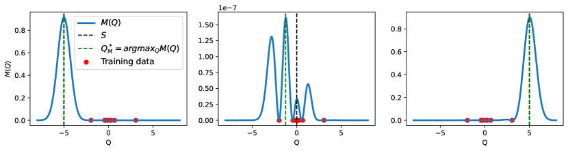
Figure 12 shows the optimal query for three different choices of . When is far from the training data (), the optimal query approximately coincides with the differing point . When is close to the training data (), the behaviour of the optimal query is non-trivial, but it should be noted that the value of the MSE is very small in this case.
Explaining when the differing point is suboptimal for Mean Distance LOOD. We now give a theoretical explanation regarding why the differing point is suboptimal for mean distance LOOD when it is close (but not so close) to the training dataset (as observed in Figure 12 middle plot). We first give a proposition that shows that the gradient of is large when the differing point is close (but not so close) to the training dataset .
Proposition 4.1.
Consider a dataset , a differing point , and a kernel function satisfying the same conditions of Theorem 3.1. Then, we have that
| (23) |
where denotes the mean distance LOOD as defined in Definition C.1, is the kernel matrix between data point and dataset , , , , and .
Proof.
The left-hand-side of Equation 23 is by definition of the mean distance LOOD in Definition C.1. This term occurs in the term in Equation 13, in the proof for Theorem 3.1. Specifically, we have . The detailed expression for is computed in line Equation 21 during the proof for Theorem 3.1. Therefore, by multiplying in Equation 21 with , we obtain the expression for in the statement Equation 23. ∎
As a result, it should be generally expected that . We can further see that when is far from the data in the sense that , the gradient is also close to . In the opposite case where is close to , e.g. satisfying , then the gradient is also close to zero. Between the two cases, there exists a region where the gradient norm is maximal.
G.2 Differing point is optimal in Mean Distance LOOD when it is far from the dataset
Explaining when the differing point is optimal for Mean Distance LOOD. We now prove that the differing point is (nearly) optimal when it is far from remaining dataset. We assume the inputs belong to some compact set .
Definition G.1 (Isotropic kernels).
We say that a kernel function is isotropic is there exists a function such that for all .
Examples includes RBF kernel, Laplace kernel, etc. For this type of kernel, we have the following result.
Lemma G.2.
Let be an isotropic kernel, and assume that its corresponding function is differentiable on (or just the interior of ). Then, for all , we have that
where
-
•
,
-
•
and
-
•
and
-
•
is a constant that depends only on .
Proof.
Let . For the sake of simplification, we use the following notation: , and .
Simple calculations yield
The first term is upperbounded by , where is the vector containing the first coordinates of , and refers to the coordinate of the vector .
Now observe that is bounded for all , provided the data labels are bounded. For this, it suffices to see that because of the positive semi-definiteness of .
Moreover, we have , which implies that . Therefore, using the triangular inequality, we obtain
The existence of is trivial. ∎
From Lemma G.2, we have the following corollary.
Corollary G.3.
Assume that , and . Then, provided that is large enough, for any and , there exists a point , such that if we define , then .
That is, if we choose far enough from the data , then the point is close to a stationary point.
Although this shows that gradient is small at (for far enough from the data ), it does not say whether this is close to a local minimum or maximum. T determine the nature of the stationary points in this region, an analysis of the second-order geometry is needed. More precisely, we would like to understand the behaviour of the Hessian matrix in a neighbourhood of . In the next result, we show that the Hessian matrix is strictly negative around (for sufficiently far from the data ), which confirms that any stationary point in the neighbourhood of should be a local maximum.
Lemma G.4 (Second-order analysis).
Assume that , , where is a negative constant that depends on the kernel function, and that . Then, provided that is large enough, for any and , there exists a point , such that if we define , then there exists satisfying: for all .
Lemma G.4.
Assume that , , where is a negative constant that depends on the kernel function, and that . Then, provided that is large enough, for any and , there exists a point , such that if we define , then there exists satisfying: for all is a negatively definite matrix.
Proof.
Let . Let . The Hessian is given by
where and . By Lemma G.2, we have that for far enough from the dataset , we have that . Therefore, the Hessian at simplilfies to the following.
For , simple calculations yield
where .
Notice that . Without loss of generality, assume that . For far enough from the dataset , we then have and . Let us now see what happens to the Hessian. For such , and for any , there exists a neighbourhood , , such that for all , we have , and . This ensures that where denotes the Frobenius norm of a matrix. On the other hand, we have . It remains to deal with . Observe that for far enough from the data , and close enough to , is close to . Thus, taking small enough, there exists satisfying the requirements, which concludes the proof. ∎
Lemma G.4 shows that whenever the point is isolated from the dataset , the Hessian is negative in a neighbourhood of , suggesting that any local stationary point can only be a local maximum. This is true for isotropic kernels such as the Radial Basis Function kernel (RBF) and the Laplace kernel. As future work, Lemma G.2 and Lemma G.4 have important computational implications for the search for the ‘worst‘ poisonous point . Finding the worst poisonous point is computationally expensive for two reasons: we cannot use gradient descent to optimize over since the target function is implicit in , and for each point , a matrix inversion is required to find . Our analysis suggests that if is far enough from the data , we can use as a lower-bound estimate of .
G.3 The optimal query for Mean Distance LOOD on image datasets
As we concluded in the analysis in Section 3, only when the differing datapoint is far away (in some notion of distance) from the rest of the dataset is the optimal query (in mean distance LOOD) the differing datapoint. In Figure 11(b), we successfully identified settings on a toy dataset where the differing point is not optimal for mean distance LOOD. We now investigate whether this also happens on an image dataset.
In Figure 13, we observe that the optimized record is indeed similar (but not identical) to the differing record for a majority fraction of cases. Therefore, also in image data the removal of a certain datapoint may influence the learned function most in a location that is not the removed datapoint itself. However, the optimized query for Mean distance LOOD still has much smaller MIA AUC score than the differing data. This again indicates that MSE optimization finds a suboptimal query for information leakage, despite achieving higher influence (mean distance).
Appendix H Deferred proofs for Section 5
Our starting point is the following observation in prior work [11], which states that the NNGP kernel is sensitive to the choice of the activation function.
Proposition H.1.
Assume that the inputs are normalized, and let denote the NNGP kernel function of a an MLP of depth . Then, the for any two inputs, we have the following
[Non-smooth activations] With ReLU: there exists a constant such that .
[Smooth activations] With GeLU, ELU, Tanh: there exists a constant such that .
As a result, for the same depth , one should expect that NNGP kernel matrix with ReLU activation is closer to a low rank constant matrix than with smooth activations such as GeLU, ELU, Tanh.888The different activations are given by
where is the c.d.f of a standard Gaussian variable, , and .
For proving Proposition 5.1, we will need the following lemma.
Lemma H.2.
Let and be two positive definite symmetric matrices. Then, the following holds
where is the smallest eigenvalue of , and is the usual -norm for matrices.
Proof.
Define the function for . Standard results from linear algebra yield
Therefore, we have
Using Weyl’s inequality on the eigenvalues of the sum of two matrices, we have the following
Combining the two inequalities concludes the proof. ∎
We are now ready to prove Proposition 5.1, as follows.
Proposition 5.1.
Let and be an arbitrary pair of leave-one-out datasets, where contains records and contains records. Define the function . Let , and thus quantifies how close the kernel matrix is to a low rank all-constant matrix. Assume that . Then, it holds that
where
and .
As a result, if and , then the maximum mean distance LOOD (i.e., maximum influence) satisfies .
Similarly, there exist constants such that
Proof.
Let be a query point and . We have the following
where and the same holds for . Let and , where is the matrix having ones everywhere. With this notation, we have the following bound
Let us deal with first term. We have that
Using Lemma H.2, we have the following
which implies that
where we have used the inequality for any two symmetric positive matrices .
Similarly, we have the following
For the last term, we have
Moreover, we have
and,
For the last term, we have
Combining all these inequalities yield the desired bound.
For the second upperbound, observe that by the definition of KL LOOD in Definition C.3. Meanwhile, for sufficiently small , we have that
and a similar formula holds for with instead of . Therefore, we obtain
Combining this result with the upperbound on the mean distance, the existence of and is straightforward. ∎