Euclid: The search for primordial features

Primordial features, in particular oscillatory signals, imprinted in the primordial power spectrum of density perturbations represent a clear window of opportunity for detecting new physics at high-energy scales. Future spectroscopic and photometric measurements from the Euclid space mission will provide unique constraints on the primordial power spectrum, thanks to the redshift coverage and high-accuracy measurement of nonlinear scales, thus allowing us to investigate deviations from the standard power-law primordial power spectrum. We consider two models with primordial undamped oscillations superimposed on the matter power spectrum described by $1+{\cal A}_{\rm X}\sin\left(\omega_{\rm X}\Xi_{\rm X}+2\pi\phi_{\rm X}\right)$, one linearly spaced in $k$-space with $\Xi_{\rm lin}\equiv k/k_{*}$ where $k_{*}=0.05\,{\rm Mpc}^{-1}$ and the other logarithmically spaced in $k$-space with $\Xi_{\rm log}\equiv\ln(k/k_{*})$. ${\cal A}_{\rm X}$ is the amplitude of the primordial feature, $\omega_{\rm X}$ is the dimensionless frequency, and $\phi_{\rm X}$ is the normalized phase, where $X=\{{\rm lin},{\rm log}\}$. We provide forecasts from spectroscopic and photometric primary Euclid probes on the standard cosmological parameters $\Omega_{\rm m,0}$, $\Omega_{\rm b,0}$, $h$, $n_{\rm s}$ and $\sigma_{8}$, and the primordial feature parameters ${\cal A}_{X}$, $\omega_{X}$ and $\phi_{X}$. We focus on the uncertainties of the primordial feature amplitude ${\cal A}_{X}$ and on the capability of Euclid to detect primordial features at a given frequency. We also study a nonlinear density reconstruction method in order to retrieve the oscillatory signals in the primordial power spectrum, which are damped on small scales in the late-time Universe due to cosmic structure formation. Finally, we also include the expected measurements from Euclid’s galaxy-clustering bispectrum and from observations of the cosmic microwave background (CMB). We forecast uncertainties in estimated values of the cosmological parameters with a Fisher matrix method applied to spectroscopic galaxy clustering (GC_sp), weak lensing (WL), photometric galaxy clustering (GC_ph), cross correlation (XC) between GC_ph and WL, spectroscopic galaxy clustering bispectrum, CMB temperature and $E$-mode polarization, temperature-polarization cross correlation, and CMB weak lensing. We consider two sets of specifications for the Euclid probes (pessimistic and optimistic) and three different CMB experiment configurations, i.e. Planck, Simons Observatory (SO) and CMB Stage-4 (CMB-S4). We find the following percentage relative errors in the feature amplitude with Euclid primary probes: for the linear (logarithmic) feature model, with a fiducial value of ${\cal A}_{X}=0.01$, $\omega_{X}=10$, $\phi_{X}=0$: 21% (22%) in the pessimistic settings and 18% (18%) in the optimistic settings at 68.3% confidence level (CL) using GC_sp+WL+GC_ph+XC. While the uncertainties on the feature amplitude are strongly dependent on the frequency value when single Euclid probes are considered, we find robust constraints on ${\cal A}_{\rm X}$ from the combination of spectroscopic and photometric measurements over the frequency range of $(1,\,10^{2.1})$. The inclusion of numerical reconstruction, GC_sp bispectrum, SO-like CMB reduces the uncertainty on the primordial feature amplitude by 32%–48%, 50%–65%, 15%–50%, respectively. Combining all the sources of information explored expected from Euclid in combination with future SO-like CMB experiment, we forecast ${\cal A}_{\rm lin}\simeq 0.010\pm 0.001$ at 68.3% CL and ${\cal A}_{\rm log}\simeq 0.010\pm 0.001$ for GC_sp(PS rec + BS)+WL+GC_ph+XC+SO-like both for the optimistic and pessimistic settings over the frequency range $(1,\,10^{2.1})$.

1 Introduction

Future galaxy surveys are the new frontier in the study of initial conditions of the Universe. They are expected to improve significantly the constraints on many of the parameters characterizing the physics of the early Universe. The Euclid satellite, performing simultaneously a spectroscopic survey of galaxies and an imaging survey (targeting weak lensing and galaxy clustering using photometric redshifts) will have the unique opportunity of measuring ultra-large scales, thanks to its large observed volume, as well as small scales of matter distribution in the full nonlinear regime. This opportunity will drastically improve our understanding of the early-Universe physics and of cosmic inflation (Starobinsky 1980; Guth 1981; Sato 1981; Linde 1982; Albrecht & Steinhardt 1982; Hawking et al. 1982; Linde 1983) through the study of the statistics hidden in the scalar density perturbations (Mukhanov & Chibisov 1981). Indeed, Euclid measurements are expected to reduce uncertainties on the amplitude of primordial scalar perturbations $A_{\rm s}$, the scalar spectral index $n_{\rm s}$ and its derivatives (or scalar runnings), the amplitude of primordial non-Gaussianity $f_{\rm NL}$ (in particular of a local type), and the spatial curvature parameter $\Omega_{K}$; and to enable us to perform significantly more stringent tests of extended models beyond single-field slow-roll inflation (Laureijs et al. 2011; Amendola et al. 2018; Euclid Collaboration: Blanchard et al. 2020).

The goal of this paper is to summarize the status of, motivations for, and challenges in searching for oscillatory features in the primordial fluctuations (see Chluba et al. 2015; Achúcarro et al. 2022, for reviews) with large-scale structure (LSS) observations expected from Euclid. Searches for primordial features based on the cosmic microwave background (CMB) angular power spectra (Wang & Mathews 2002; Adams et al. 2001; Peiris et al. 2003; Mukherjee & Wang 2003; Covi et al. 2006; Hamann et al. 2007; Meerburg et al. 2012; Planck Collaboration: Ade et al. 2014b; Meerburg et al. 2014; Benetti 2013; Miranda & Hu 2014; Easther & Flauger 2014; Chen & Namjoo 2014; Achúcarro et al. 2014; Hazra et al. 2014a, b; Hu & Torrado 2015; Planck Collaboration: Ade et al. 2016b; Gruppuso & Sagnotti 2015; Gruppuso et al. 2016; Hazra et al. 2016; Torrado et al. 2017; Planck Collaboration: Akrami et al. 2020a; Zeng et al. 2019; Cañas-Herrera et al. 2021; Braglia et al. 2021, 2022b, 2022a; Naik et al. 2022; Hamann & Wons 2022) and bispectra (Planck Collaboration: Ade et al. 2014a; Fergusson et al. 2015; Planck Collaboration: Ade et al. 2016a; Meerburg et al. 2016; Planck Collaboration: Akrami et al. 2020a, b) have so far not detected any statistically significant signal, setting constraints on deviations from a pure power-law primordial power spectrum (PPS) at the few percent level (depending on the methodology applied) for wavenumbers in the range $0.005<k/(h\,{\rm Mpc}^{-1})<0.2$. However, it is important to stress that there are interesting models of primordial features that are able to reproduce some of the anomalous features observed in the CMB temperature angular power spectrum at a marginal statistical significance of 99.7%. These include the dip in power in the multipole range $\ell\sim 20$–40 and an oscillatory pattern at the intermediate scales $\ell\sim 700$–800. Models with primordial features have also been studied in the context of the anomalous CMB lensing smoothing excess, as well as the $H_{0}$ and $S_{8}$ tensions (Planck Collaboration: Akrami et al. 2020a; Domènech & Kamionkowski 2019; Liu & Huang 2020; Domènech et al. 2020; Keeley et al. 2020; Hazra et al. 2022; Antony et al. 2023; Ballardini & Finelli 2022).

In the context of primordial features, large-volume photometric and spectroscopic surveys not only provide a complementary look at the structure on very large scales, but they can also provide a precise measurement of the power spectrum on small scales, complementing the CMB measurements and improving the sensitivity for high-frequency signals. This has been studied extensively with forecast analyses in Wang et al. (1999); Zhan et al. (2006); Huang et al. (2012); Chen et al. (2016a, b); Ballardini et al. (2016); Xu et al. (2016); Ansari Fard & Baghram (2018); Palma et al. (2018); Ballardini et al. (2018); Ballardini (2019); Beutler et al. (2019); Ballardini et al. (2020); Debono et al. (2020); Li et al. (2022) and demonstrated on real data in Beutler et al. (2019); Ballardini et al. (2023); Mergulhão et al. (2023) showing that current galaxy clustering data of the Baryon Oscillation Spectroscopic Survey (BOSS) alone can already provide constraints that are competitive with those derived from the Planck CMB data. Given the potential of the Euclid mission, it is imperative to have a good description of the LSS observables on all observed scales, and to do so, nonlinear corrections need to be correctly accounted for (Vlah et al. 2016; Vasudevan et al. 2019; Beutler et al. 2019; Ballardini et al. 2020; Chen et al. 2020; Li et al. 2022; Ballardini & Finelli 2022).

In this paper, we forecast how well the surveys from the Euclid mission can constrain two templates of primordial undamped linear and logarithmic oscillations. In addition to the Euclid’s primary probes, i.e. the spectroscopic galaxy clustering and the combination of photometric surveys, we study the further constraints that will be added by Euclid’s measurements of the galaxy bispectrum and the information provided by future CMB experiments. The bispectrum is shown to be able to provide essential information on the parameters of the feature models, highlighting the importance of a high-order statistics analysis on the spectroscopic sample.

We structure the paper as follows. In Sect. 2, we introduce the physics of the adiabatic mode and we briefly review the diverse theoretical mechanisms that naturally generate features in the PPS, in particular realizations of inflation. In Sect. 3, we review Euclid specifications and calculation of the theoretical observables used in the Fisher forecast analysis. In Sect. 4 we start introducing the parametrized templates for primordial features with linear and logarithmic undamped oscillations. We then study the behaviour of these models on nonlinear scales of the matter power spectrum comparing the results from perturbation theory in Sect. 4.2 to N-body simulations in Sect. 4.3, and we study the numerical reconstruction of primordial features in Sect. 4.4. We present our results from primary Euclid observables in Sect. 5. We complement those by adding the information from the galaxy bispectrum in Sect. 6 and combining Euclid results with future CMB measurements in Sect. 7. We conclude in Sect. 8.

2 Primordial features and the early Universe

As mentioned in Sect. 1, the search for features in the primordial power spectrum has so far been statistically unsuccessful. On the largest scales, CMB observations agree with a red-tilted power-law PPS, ${\cal P}_{{\cal R},\,0}(k)$, with the following parametrization

$${\cal P}_{{\cal R},\,0}(k)=A_{\rm s}\left(\frac{k}{k_{*}}\right)^{n_{\rm s}-1}\,,$$ (1)

where $A_{\rm s}$ and $n_{\rm s}$ are the amplitude and the spectral index of the comoving curvature perturbations ${\cal R}$ on superhorizon scales at the pivot scale $k_{*}=0.05\,{\rm Mpc}^{-1}$.

The simplest class of models that can produce such a spectrum is known as canonical single-field slow-roll inflation. In these models a single scalar field — the inflaton — is responsible for both the primordial perturbations and the background evolution during inflation.

Unless the inflaton is the Higgs field (Bezrukov & Shaposhnikov 2008), inflation always takes us beyond the Standard Model (SM) of particle physics. While these scenarios can support cosmic inflation, it is rarely of the simplest kind. Beyond-SM models often involve multiple fields that interact with each other, and with the inflaton, and they can leave detectable imprints on the primordial perturbations including, e.g. isocurvature modes and localised features. It is essential to have a bottom-up theoretical framework enabling us to analyse and classify all possible departures from the simplest scenario of Eq. (1) that are compatible with observations. Here we focus on the fluctuations as those are what we observe in the CMB and LSS. An important distinction is whether the curvature perturbations on superhorizon scales are generated by a single, possibly effective, degree of freedom. These are called effectively single field or ‘single clock’ models.

It can be shown that in the effective single-field slow-roll models the effective action for the comoving curvature perturbations is, to quadratic order,

$$S=\int{{\rm d}^{4}x\,a^{3}M_{\mathrm{Pl}}^{2}\epsilon_{1}\left[\frac{\dot{\mathcal{R}}^{2}}{c_{\rm s}^{2}}-\frac{(\partial_{i}\mathcal{R})^{2}}{a^{2}}\right]}+\dots\,,$$ (2)

where $a(t)$ is the scale factor, $c_{\rm s}(t)$ is the speed of sound for curvature perturbations, and $\epsilon_{1}(t)\equiv-\dot{H}/H^{2}$ is the first slow-roll parameter; $H\equiv\dot{a}/a$ is the Hubble expansion rate, where the overdot denotes derivative with respect to the cosmic time $t$.

Eq. (2) is well known in the context of single-field slow-roll inflation, but it is much more general than that. It is the first term in a perturbative expansion — the effective field theory (EFT) of inflationary perturbations (Cheung et al. 2008) — where all the information about the background is systematically encoded in a set of functions ($\epsilon_{1}$ and $c_{\rm s}$ being the first two) that describe what is seen by the perturbations.

This action describes almost all models of slow-roll inflation in which the primordial perturbations are generated by a single quantum field. It includes canonical single-field slow-roll models as a particular case ($c_{\rm s}=1$) but also any multi-field model in which the primordial perturbations are generated by a single quantum field (typically an effective low energy degree of freedom involving multiple high energy fields). The action in Eq. (2) is then obtained by integrating out the fast, or heavy, high energy degrees of freedom; see Achúcarro et al. (2012).

The idea behind the EFT approach is that what the perturbations see is an almost time-independent background, and this symmetry under time translations completely dictates the form of the action in Eq. (2), to all orders. The red tilt is a small deviation from perfect scale invariance, measured by the smallness of the slow-roll parameters. Any deviations from time-independence in the background functions result in features in the spectrum that can be calculated and cross-correlated among different observables; see Bartolo et al. (2013); Cannone et al. (2014) for applications of the EFT in the context of primordial oscillatory features.

In general, and depending on their origin, oscillatory features fall into two main classes which are the focus of this paper (see Achúcarro et al. 2022, for details and references). A small, abrupt change in the background functions $\epsilon_{1}(t)$ and $c_{\rm s}(t)$ at a particular moment during inflation results in a transient oscillatory feature, linearly spaced in $k$, superimposed on the power spectrum (1). Two well studied examples are a step in the inflationary potential (Starobinsky 1992; Adams et al. 2001) and a localised turn in the inflationary trajectory (Achúcarro et al. 2011; Chen 2011). The range of $k$ where the oscillation persists increases with the sharpness of the change. But the sharpness cannot be arbitrarily large, since it should not excite the high energy modes that have been integrated out, nor enhance higher order terms that have been neglected in the perturbative expansion. On the other hand, oscillations logarithmically spaced in $k$ are usually associated with periodicity in the background functions, for instance if there is a periodic modulation in the inflationary potential (Freese et al. 1990; Chen et al. 2008). More complicated combinations are also possible, that require a more tailored analysis. The upshot is that, if a feature is detected in the power spectrum, establishing its high energy origin will require stringent self-consistency checks, as well as correlated detections in other observables.

It is worth emphasising that the power of the EFT approach is that, since it is completely agnostic about the origin of the background expansion, it tests entire classes of models as opposed to individual ones. For example in multi-field models, $\epsilon_{1}$ is related to the flatness of the potential along the inflationary trajectory, and $c_{\rm s}$ is related to the rate of turning of this trajectory in multi-field space. But the high energy origin of $\epsilon_{1}$ and $c_{\rm s}$ may be completely different in other models.

3 Euclid probes

Euclid is one of the next generation deep- and large-field galaxy surveys. It will be able to measure up to $30$ million spectroscopic redshifts, which can be used for galaxy clustering measurements, and $2$ billion photometric galaxy images, which can be used for weak lensing observations.

Euclid will use near-IR (NIR) slitless spectroscopy to collect large samples of emission-line galaxies and to perform spectroscopic galaxy clustering measurements. The great advantage of this spectroscopic method is the high precision on measuring the redshift of the sources. However, one of the difficulties in inferring the cosmological parameters is given to the knowledge of the number density of the $H\alpha$ targets. The total number of galaxies that can be used in the analysis mostly depends on two factors: completeness and purity. Completeness is the fraction of objects correctly identified relative to the true number, whereas purity is defined as the fraction of objects correctly identified relative to the total number of detected objects. In practice, completeness represents the size of a sample, whereas purity is its quality. A lower value of the number density $n(z)$ of observed galaxies leads to an increase of the shot noise, resulting as a degradation on the constraints of the cosmological parameters.

One of the expected lensing observations is the cosmic shear, which is the distortion in the observed shapes of distant galaxies due to weak gravitational lensing by the LSS while the other probe comes from galaxy clustering using the positions of objects detected by the photometric measurements of redshifts. Given that both depend on the LSS density fluctuations as well as the geometry of the Universe, this will allow us to constrain the cosmological parameters. One of the main difficulties in using the weak lensing observable is the ability to accurately model the intrinsic alignments (IA) of galaxies that mimic the cosmological lensing signal. While for the galaxy clustering from photometric measurements, the main effects that need to be taken into account are the galaxy bias, accounting for the relation between the galaxy distribution and the underlying total matter distribution, and the photometric-redshift uncertainties, since redshift in this case is estimated from observing through multi-band filters instead of the full spectral energy distribution. Finally, an important issue for both the weak lensing and galaxy clustering probes is the modelling of the small-scale nonlinear clustering on the weak lensing two-point statistics that the high density of detected galaxies will allow us to reach.

In the following we detail on the prescription used in this work for our model for these two probes.

3.1 Spectroscopic galaxy clustering

Following Euclid Collaboration: Blanchard et al. (2020), we define the observed galaxy power spectrum as

$$P_{\text{obs}}(k_{\rm ref},\mu_{\rm ref};z)= \frac{1}{q_{\perp}^{2}q_{\parallel}}\frac{1}{1+k^{2}\mu^{2}f^{2}(z)\sigma_{\rm p}^{2}(z)}$$

$$\times\left[b(z)\sigma_{8}(z)+f(z)\sigma_{8}(z)\mu^{2}\right]^{2}$$

$$\times\frac{P^{\rm IR\,res,\,LO}(k,\mu;z)}{\sigma^{2}_{8}(z)}F_{z}(k,\mu;z)$$

$$+P_{\rm s}(z)\,,$$ (3)

where $\mu$ is the cosine of the angle of the wave mode with respect to the line of sight pointing into the direction $\hat{r}$. Here $b(z)$ is the linear clustering bias, $f(z)$ is the growth rate, and $\sigma_{8}(z)$ is the root mean square linearly evolved density fluctuations in spheres of $8\,h^{-1}\,{\rm Mpc}$.

The Alcock-Paczynski (AP) effect (Alcock & Paczynski 1979), used to account for deviations of the cosmological models from the fiducial one, is parametrized through rescaling of the angular diameter distance $D_{\rm A}(z)$ and the Hubble parameter $H(z)$, and enters as multiplicative factor through

$$q_{\perp}(z)=\frac{D_{\rm A}(z)}{D_{\rm A,\,ref}(z)}\qquad\text{and}\qquad q_{\parallel}(z)=\frac{H_{\rm ref}(z)}{H(z)}\,,$$ (4)

where the subscript $\rm ref$ refers to the fiducial cosmology. This leads also to a rescaling of the wavevector components as

$$k_{\perp}=\frac{k_{\perp,{\rm ref}}}{q_{\perp}}\qquad\text{and}\qquad k_{\parallel}=\frac{k_{\parallel,{\rm ref}}}{q_{\parallel}}\,.$$ (5)

Using Eqs. (4) and (5) we can convert the known reference cosmology ($k_{\rm ref}$ and $\mu_{\rm ref}$) to the true unknown cosmology ($k$ and $\mu$),

$$k(k_{\rm ref},\mu_{\rm ref})=k_{\rm ref}\alpha(\mu_{\rm ref})\,,$$ (6)

$$\mu(\mu_{\rm ref})=\frac{\mu_{\rm ref}}{\alpha(\mu_{\rm ref})q_{\parallel}}\,,$$ (7)

where

$$\alpha(\mu)=\left[\frac{\mu^{2}}{q_{\parallel}^{2}}+\frac{\left(1-\mu^{2}\right)}{q_{\perp}^{2}}\right]^{1/2}\,.$$ (8)

The relations above can be used to define the effect of the choice of reference cosmology on the observed power spectrum via

$$P_{\rm obs}(k_{\rm ref},\mu_{\rm ref};z)=\frac{1}{q_{\perp}^{2}q_{\parallel}}P_{\rm g}\left(k(k_{\rm ref}),\mu(\mu_{\rm ref});z\right)\,.$$ (9)

Galaxy bias, connecting the underlying dark matter (DM) power spectrum to the $H\alpha$-line emitter galaxies detected by Euclid, is modelled by a simple linear clustering bias redshift-dependent coefficient $b(z)$. The anisotropic distortion to the density field due to the line-of-sight effects of the peculiar velocity of the observed galaxy redshifts, known as redshift-space distortions (RSD), is modelled in the linear regime by the contribution in the square brackets introduced by Kaiser (1987). Linear RSD are corrected for the nonlinear finger-of-God (FoG) effect under the assumption of an exponential galaxy velocity distribution function as a Lorentzian (Hamilton 1998). The nonlinearities due to gravitational instabilities have the effect of smearing the baryon acoustic oscillations (BAO) signal, this is modelled through time-sliced perturbation theory (TSPT); we discuss the modelling of $P^{\rm IR\,res,\,LO}$ in Sect. 4.2. The pairwise velocity dispersion, $\sigma_{\rm p}(z)$, is evaluated from the linear matter power spectrum as

$$\sigma^{2}_{\rm p}(z)=\frac{1}{6\pi^{2}}\int_{0}^{k_{\rm max}}{\rm d}k\,P_{\rm lin}(k,z)\,.$$ (10)

The total galaxy power spectrum in Eq. (3.1) includes errors on the measurement of the redshift through the exponential factor

$$F_{z}(k,\mu;z)=\text{e}^{-k^{2}\mu^{2}\sigma_{r}^{2}(z)}\,,$$ (11)

where $\sigma_{r}^{2}(z)=c(1+z)\sigma_{0,z}/H(z)$ with $\sigma_{0,z}$ the error on the measured redshifts. Finally, we introduce a shot-noise term $P_{\rm s}(z)$ due to imperfect removal of the Poisson sampling and the imperfect modelling of small scales.

The final Fisher matrix for the spectroscopic galaxy clustering (GC_sp) observable for one redshift bin $z_{i}$ is

$$F_{\alpha\beta}(z_{i}) = \frac{1}{8\pi^{2}}\int_{-1}^{1}{\rm d}\mu\int_{k_{\rm min}}^{k_{\rm max}}k^{2}{\rm d}kV_{\rm eff}(z_{i},k)$$ (12)

$$\times\frac{\partial\ln P_{\rm obs}(k,\mu;\,z_{i})}{\partial\theta_{\alpha}}\frac{\partial\ln P_{\rm obs}(k,\mu;\,z_{i})}{\partial\theta_{\beta}}\,,$$

where the derivatives are evaluated at the parameter values of the fiducial model and $V_{\rm eff}$ is the effective volume of the survey, given by

$$V_{\rm eff}(k,\mu;\,z)=V_{\rm s}\left[\frac{n(z)P_{\rm obs}(k,\mu;\,z)}{1+n(z)P_{\rm obs}(k,\mu;\,z)}\right]^{2}\,,$$ (13)

where $V_{\rm s}$ is the volume of the survey and $n(z)$ is the number of galaxies in a redshift bin. Assuming that the observed power spectrum follows a Gaussian distribution, we write in Eq. (12) its covariance matrix as

$${\rm Cov}(k,k^{\prime})\approx\frac{2(2\pi)^{3}}{V_{\rm eff}(k,\mu;\,z)}P_{\rm obs}^{2}(k,\mu;\,z)\delta^{\rm D}(k-k^{\prime})\,,$$ (14)

where $\delta^{\rm D}(k-k^{\prime})$ is the Dirac delta function.

We model the observed matter power spectrum of Eq. (3.1) in bandpowers averaged over a bandwidth of $\Delta k$ with a top-hat window function as in Huang et al. (2012); Ballardini et al. (2016),

$$\hat{P}_{\rm obs}(k,\mu;\,z)=\frac{1}{\Delta k}\int^{k+\Delta k/2}_{k-\Delta k/2}{\rm d}k^{\prime}P_{\rm obs}(k^{\prime},\mu;\,z)\,.$$ (15)

The size of the $k$-bin $\Delta k$ should be equal or larger than the effective fundamental frequency defined as $k_{\rm eff}\equiv 2\pi/V^{1/3}$ for an ideal cubic volume in order to guarantee uncorrelated measurements of the observed power spectrum. The values of $k_{\rm eff}$ span in the range 0.0025–$0.0031\,h\,{\rm Mpc}^{-1}$ for a cubic volume for the four redshift bins. We assume a bin width of $\Delta k=0.004\,h\,{\rm Mpc}^{-1}$ with $k_{\rm min}=0.002\,h\,{\rm Mpc}^{-1}$. Finally, we can rewrite the Fisher matrix of Eq. 12 for the discrete number of averaged bandpower for the redshift bin $z_{i}$ as

$$F_{\alpha\beta}(z_{i})= \frac{1}{8\pi^{2}}\int_{-1}^{1}{\rm d}\mu\sum_{k=k_{\rm min}}^{k_{\rm max}}k^{2}\Delta kV_{\rm eff}(z_{i},k)$$

$$\times\frac{\partial\ln\hat{P}_{\rm obs}(k,\mu;\,z_{i})}{\partial\theta_{\alpha}}\frac{\partial\ln\hat{P}_{\rm obs}(k,\mu;\,z_{i})}{\partial\theta_{\beta}}\,.$$ (16)

The total spectroscopic Fisher matrix is then calculated by summing over the redshift bins as $F_{\alpha\beta}^{\rm sp}=\sum_{i}F_{\alpha\beta}(z_{i})$, assuming that the redshift bins are independent. Since we are interested in the standard cosmological parameters and the feature parameters, we marginalise the GC_sp Fisher matrix over two redshift-dependent parameters $b\sigma_{8}(z_{i})$ and $P_{\rm s}(z_{i})$ for each of the four redshift bins.

3.2 Photometric galaxy clustering and weak lensing

Both the forecasting method and the tools used for the photometric analyses are the same as the ones in Euclid Collaboration: Blanchard et al. (2020) apart from the changes in the power spectrum due to the primordial features in the predicted Euclid observables. Here we only remind the reader of the main steps.

The observables we consider are the angular power spectra $C_{ij,\ell}^{XY}$ between probe $X$ in the $i$-th redshift bin and probe $Y$ in the $j$-th redshift bin, where the probes $X$ and $Y$ are L for weak lensing or G for photometric galaxy clustering; $C_{ij,\ell}^{XY}$ therefore refers to both auto- and cross-correlations of these probes. Relying on the Limber approximation and within the flat sky limit, the spectra are given by

$$C^{XY}_{ij,\ell}=c\int_{z_{\rm min}}^{z_{\rm max}}\mathrm{d}z\,{\frac{W_{i}^{X}(z)W_{j}^{Y}(z)}{H(z)r^{2}(z)}P_{\rm NL}(k_{\ell},z)}\,,$$ (17)

with $k_{\ell}=(\ell+1/2)/r(z)$, $r(z)$ the comoving distance to redshift $z$, and $P_{\rm NL}(k_{\ell},z)$ the nonlinear power spectrum of matter density fluctuations at wave number $k_{\ell}$ and redshift $z$. The GC_ph  and WL window functions read

$$W_{i}^{\rm G}(z)= \;b_{i}(z)\,n_{i}(z)\frac{H(z)}{c}\,,$$ (18)

$$W_{i}^{\rm L}(z)= \;\frac{3}{2}\Omega_{\mathrm{m},0}\left(\frac{H_{0}}{c}\right)^{2}(1+z)\,r(z)\,\int_{z}^{z_{\rm max}}{\mathrm{d}z^{\prime}n_{i}(z^{\prime})\left[1-\frac{r(z)}{r(z^{\prime})}\right]}$$

$$+W^{\rm IA}_{i}(z)\,,$$ (19)

where $b_{i}(z)$ is the galaxy bias in the $i$-th redshift bin, and $W^{\rm IA}_{i}(z)$ encodes the contribution of IA to the WL power spectrum. The normalised number density distribution $n_{i}(z)$ of observed galaxies in the $i$-th redshift bin is given by

$$n_{i}(z)=\frac{\int_{z_{i}^{-}}^{z_{i}^{+}}\mathrm{d}z^{\prime}n(z)p_{\rm ph}(z^{\prime}|z)}{\int_{z_{\rm min}}^{z_{\rm max}}\mathrm{d}z\int_{z_{i}^{-}}^{z_{i}^{+}}\mathrm{d}z^{\prime}n(z)p_{\rm ph}(z^{\prime}|z)}\,,$$ (20)

where $(z_{i}^{-},z_{i}^{+})$ are the edges of the $i$-th redshift bin and $n(z)$ is the underlying true redshift distribution. The true number density of galaxies is convolved with the probability distribution function $p_{\rm ph}(z^{\prime}|z)$ is given following the parameterization in Euclid Collaboration: Blanchard et al. (2020).

The IA contribution is computed following the extended nonlinear alignment (eNLA) model adopted in Euclid Collaboration: Blanchard et al. (2020) so that the corresponding window function is

$$W^{\rm IA}_{i}(z)=-\frac{\mathcal{A}_{\rm IA}\,\mathcal{C}_{\rm IA}\,\Omega_{\rm m,0}\,\mathcal{F}_{\rm IA}(z)}{D(z)}n_{i}(z)\frac{H(z)}{c}\,,$$ (21)

where

$$\mathcal{F}_{\rm IA}(z)=(1+z)^{\eta_{\rm IA}}\left[\frac{\langle L\rangle(z)}{L_{\star}(z)}\right]^{\beta_{\rm IA}}\,,$$ (22)

with $\langle L\rangle(z)$ the redshift-dependent mean, and $L_{\star}(z)$ the characteristic luminosity of source galaxies as computed from the luminosity function. $\mathcal{A}_{\rm IA}$, $\beta_{\rm IA}$ and $\eta_{\rm IA}$ are the nuisance parameters of the model, and $\mathcal{C}_{\rm IA}$ is a constant accounting for dimensional units.

We consider a Gaussian-only covariance whose elements are given by

$$\text{Cov}\left[C_{ij,\ell}^{\rm AB},C_{mn,\ell^{\prime}}^{\rm CD}\right]= \frac{\delta_{\ell\ell^{\prime}}^{\rm K}}{(2\ell+1)f_{\rm sky}\Delta\ell}$$

$$\times\left\{\left[C_{im,\ell}^{\rm AC}+{\cal N}_{im,\ell}^{\rm AC}\right]\left[C_{jn,\ell^{\prime}}^{\rm BD}+{\cal N}_{jn,\ell^{\prime}}^{\rm BD}\right]\right.$$

$$+\left.\left[C_{in,\ell}^{\rm AD}+{\cal N}_{in,\ell}^{\rm AD}\right]\left[C_{jm,\ell^{\prime}}^{\rm BC}+{\cal N}_{jm,\ell^{\prime}}^{\rm BC}\right]\right\}\,,$$ (23)

where the upper- and lower-case Latin indices run over L and G (all tomographic bins), $\delta_{\ell\ell^{\prime}}^{\rm K}$ is the Kronecker delta coming from the lack of correlation between different multipoles $(\ell,\ell^{\prime})$, $f_{\rm sky}$ is the survey’s sky fraction, and $\Delta\ell$ denotes the width of the logarithmic equi-spaced multipole bins. We consider a white noise,

$${\cal N}_{ij,\ell}^{\rm LL} =\frac{\delta_{ij}^{\rm K}}{\bar{n}_{i}}\sigma_{\epsilon}^{2}\,,\quad{\cal N}_{ij,\ell}^{\rm GG}=\frac{\delta_{ij}^{\rm K}}{\bar{n}_{i}}\,,\quad{\cal N}_{ij,\ell}^{\rm GL}=0\,,$$ (24)

where $\sigma_{\epsilon}$ is the variance of observed ellipticities.

For evaluating the Fisher matrix $F_{\alpha\beta}^{\rm ph}$ for the observed galaxy power spectrum, we use

$$F_{\alpha\beta}^{\rm ph}=\sum_{\ell=\ell_{\rm min}}^{\ell_{\rm max}}\sum_{ij,mn}\frac{\partial C_{ij,\ell}^{\rm AB}}{\partial\theta_{\alpha}}\text{Cov}^{-1}\left[C_{ij,\ell}^{\rm AB},C_{mn,\ell}^{\rm CD}\right]\frac{\partial C_{mn,\ell}^{\rm CD}}{\partial\theta_{\beta}}\,.$$ (25)

3.3 Survey specifications

Following Euclid Collaboration: Blanchard et al. (2020), we consider for the spectroscopic sample four redshift bins centred at $\{1.0,1.2,1.4,1.65\}$, whose widths are $\Delta z=0.2$ for the first three bins and $\Delta z=0.3$ for the last bin. The H$\alpha$ bias, evaluated at the central redshift of the bins, corresponds to $\{1.46,1.61,1.75,1.90\}$. The number density of galaxies $n(z)$ corresponds to $\{6.86,5.58,4.21,2.61\}\times 10^{-4}$.

For the photometric probes, the sources are split into 10 equi-populated redshift bins whose limits are obtained from the redshift distribution

$$n(z)\propto\left(\frac{z}{z_{0}}\right)^{2}\,\text{exp}\left[-\left(\frac{z}{z_{0}}\right)^{3/2}\right]\,,$$ (26)

with $z_{0}=0.9/\sqrt{2}$ and the normalisation set by the requirement that the surface density of galaxies is $\bar{n}_{g}=30\,\mathrm{arcmin}^{-2}$. This is then convolved with the sum of two Gaussians to account for the effect of photometric redshift (see Euclid Collaboration: Blanchard et al. 2020, for details). The galaxy bias is assumed to be constant within each redshift bin, with fiducial values $b_{i}=\sqrt{1+\bar{z}_{i}}$, where $\bar{z}_{i}$ is the bin centre. We consider $100$ logarithmic equi-spaced multipole bins with $\sigma_{\epsilon}=0.3$ the variance of observed ellipticities. We set $(z_{\rm min},z_{\rm max})=(0.001,4)$, which spans the full range where the source redshift distributions $n_{i}(z)$ are non-vanishing.

For all the Euclid probes the survey’s sky fraction is $f_{\rm sky}\simeq 0.36$ (Euclid Collaboration: Scaramella et al. 2022).

4 Theoretical modelling of primordial features in galaxy surveys

As representative models for features in primordial fluctuations in this paper we consider oscillations linearly and logarithmically spaced in Fourier space with a constant amplitude superimposed to a power spectrum described by a power-law.

4.1 Models

We consider a superimposed pattern of oscillations as

$${\cal P}_{\cal R}(k)={\cal P}_{{\cal R},\,0}(k)\left[1+\delta P^{\rm X}(k)\right]\,,$$ (27)

where ${\cal P}_{{\cal R},\,0}(k)$ is the standard power-law PPS of the comoving curvature perturbations $\cal R$ on superhorizon scales, given in Eq. (1). We study the following templates with superimposed oscillations on the PPS

$$\delta P^{\rm X}(k)={\cal A}_{\rm X}\sin\left(\omega_{\rm X}\Xi_{\rm X}+2\pi\phi_{\rm X}\right)\,,$$ (28)

where ${\rm X}=\{{\rm lin,\,log}\}$ and $\Xi_{\rm X}=\{k/k_{*},\,\ln(k/k_{*})\}$.

We choose the fiducial cosmological parameters according to Planck DR3 mean values of the marginalised posterior distributions (Planck Collaboration: Aghanim et al. 2020b): $\omega_{\rm b}=0.02237$, $\omega_{\rm c}=0.1200$, $H_{0}=67.36\,$\mathrm{km}\text{\,}{\mathrm{s}}^{-1}\text{\,}{\mathrm{Mpc}}^{-1}$$, $\ln(10^{10}A_{\rm s})=3.044$, $n_{\rm s}=0.9649$, $\sigma_{8}=0.8107$, and $m_{\nu}=0.06$ $\mathrm{e}\mathrm{V}$ (with one massive neutrino and two massless ones). In what follows we specify the fiducial values of the model parameters.

1. Linear oscillations:

   $$\Theta_{\rm lin}=\Bigl{\{}{\cal A}_{\rm lin}=0.01,\,\omega_{\rm lin}=10,\,\phi_{\rm lin}=0\Bigr{\}}\,.$$ (29)

2. Logarithmic oscillations:

   $$\Theta_{\rm log}=\Bigl{\{}{\cal A}_{\rm log}=0.01,\,\omega_{\rm log}=10,\,\phi_{\rm log}=0\Bigr{\}}\,.$$ (30)

We show the effect of the feature parameters on the PPS in Fig. 1.

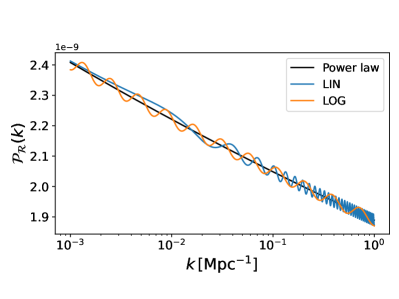
Figure 1: Primordial power spectrum of curvature perturbations for linear (LIN) and logarithmic (LOG) feature models with fiducial parameter values given in (29) and (30).

4.2 Modelling nonlinear scales in perturbation theory in the presence of primordial oscillatory features

The linearly propagated matter power spectrum is given by

$$P_{\rm lin}(k,z)=M^{2}(k,z)P_{\Phi}(k)\,,$$ (31)

where $M(k,z)=2k^{2}c^{2}T(k)D(z)/(3\Omega_{\rm m}H_{0}^{2})$, with $T(k)$ the matter transfer function normalised to unity at large scales (i.e. $k\rightarrow 0$) and $c$ the speed of light. The gravitational potential power spectrum will then be derived from the two oscillatory models considered: $P_{\Phi}=9/25(2\pi^{2}){\cal P}_{\cal R}(k)/k^{3}$.

Our analytic model for the matter power spectrum is based on TSPT and it takes into account the damping of oscillations by infrared (IR) resummation of the large-scale bulk flows (Crocce & Scoccimarro 2008; Creminelli et al. 2014; Baldauf et al. 2015; Blas et al. 2016b; Senatore & Trevisan 2018). The implementation of the IR resummation can be done following the approach to BAO in the context of TSPT (Blas et al. 2016a, b). We start by decomposing the linear matter power spectrum into a smooth (or no-wiggle; nw) and an oscillating (w) contribution,

$$P_{\rm lin}(k,z)=D^{2}(z)\left[P_{\rm nw}(k)+P_{\rm w}(k)\right]\,,$$ (32)

where $P_{\rm nw}$ is the no-wiggle power spectrum, and the oscillatory part $P_{\rm w}$ describes both the BAO feature and the primordial oscillating feature as

$$P_{\rm w}(k)\equiv P_{\rm nw}\left[\delta P_{\rm w}^{\rm BAO}(k)+\delta P_{\rm w}^{\rm X}(k)+\delta P_{\rm w}^{\rm BAO}(k)\delta P_{\rm w}^{\rm X}(k)\right]\,.$$ (33)

Here we have factored out the time-dependence given by the growth factor $D(z)$. We have neglected the cross term in Eq. (33) as it is proportional to $A_{\rm BAO}\times{\cal A}_{\rm lin}$ and therefore subdominant. We filter the BAO feature from the linear matter power spectrum using a Savitzky-Golay filter; see Boyle & Komatsu (2018).

At next-to-leading order (NLO), the IR resummed power spectrum for linear oscillations can be written as (Blas et al. 2016b; Beutler et al. 2019)

$$P^{\rm IR\,res,\,LO+NLO}(k,z)=D^{2}(z)P_{\rm nw}(k)$$

$$\qquad\times\left\{1+\left[1+k^{2}D^{2}(z)\Sigma^{2}_{\rm BAO}\right]\mathrm{e}^{-k^{2}D^{2}(z)\Sigma^{2}_{\rm BAO}}\delta P_{\rm w}^{\rm BAO}(k)\right.$$

$$\qquad\left.+\left[1+k^{2}D^{2}(z)\Sigma^{2}_{\rm lin}\right]\mathrm{e}^{-k^{2}D^{2}(z)\Sigma^{2}_{\rm lin}}\delta P_{\rm w}^{\rm lin}(k)\right\}$$

$$\qquad+D^{4}(z)P^{\rm 1-loop}\left[P^{\rm IR\,res,\,LO}(k)\right]\,,$$ (34)

and for logarithmic oscillations as (Vasudevan et al. 2019; Beutler et al. 2019)

$$P^{\rm IR\,res,\,LO+NLO}(k,z)=D^{2}(z)P_{\rm nw}(k)$$

$$\qquad\times\Biggl{\{}1+\left[1+k^{2}D^{2}(z)\Sigma^{2}_{\rm BAO}\right]\mathrm{e}^{-k^{2}D^{2}(z)\Sigma^{2}_{\rm BAO}}\delta P_{\rm w}^{\rm BAO}(k)$$

$$\qquad+\left[1+k^{2}D^{2}(z)\Sigma^{2}_{\rm log}\right]\mathrm{e}^{-k^{2}D^{2}(z)\Sigma^{2}_{\rm log}}\biggl{[}\cos\left(k^{2}D^{2}(z)\hat{\Sigma}_{\rm log}^{2}\right)\delta P_{\rm w}^{\rm log}(k)$$

$$\qquad-\sin\left(k^{2}D^{2}(z)\hat{\Sigma}^{2}_{\rm log}\right)\frac{{\rm d}\,\delta P_{\rm w}^{\rm log}(k)}{\omega_{\rm log}\,{\rm d}\,\ln\,k}\biggr{]}\Biggr{\}}$$

$$\qquad+D^{4}(z)P^{\rm 1-loop}\left[P^{\rm IR\,res,\,LO}(k)\right]\,.$$ (35)

$P^{\rm 1-loop}$ is the standard one-loop result, but computed with the leading-order (LO) IR resummed power spectrum. We take the usual expression $P^{\rm 1-loop}=P_{22}+2P_{13}$ with

$$P_{22}(k)=\int\frac{{\rm d}^{3}q}{4\pi^{3}}F_{2}^{2}({\bf q},{\bf k}-{\bf q})P_{\rm lin}(q)P_{\rm lin}(|{\bf k}-{\bf q}|)\,,$$ (36)

$$P_{13}(k)=3P_{\rm lin}(k)\int\frac{{\rm d}^{3}q}{4\pi^{3}}F_{3}({\bf q},-{\bf q},{\bf k})P_{\rm lin}(q)\,,$$ (37)

while evaluating the loop integrals $P_{22}$ and $P_{13}$ with the input spectrum $P^{\rm IR\,res,\,LO}$ instead of the linear spectrum (Blas et al. 2016a). $F_{n}$ are the usual perturbation theory (PT) kernels (Bernardeau et al. 2002). We calculate these quantities, i.e. Eqs. (36) and (37), with the publicly available code FAST-PT (McEwen et al. 2016; Fang et al. 2017). The IR resummed power spectrum at leading order is given by

$$P^{\rm IR\,res,\,LO}(k,z)=D^{2}(z)P_{\rm nw}(k)$$

$$\qquad\times\left[1+\mathrm{e}^{-k^{2}D^{2}(z)\Sigma^{2}_{\rm BAO}}\delta P_{\rm w}^{\rm BAO}(k)+\mathrm{e}^{-k^{2}D^{2}(z)\Sigma^{2}_{\rm lin}}\delta P_{\rm w}^{\rm lin}(k)\right]$$ (38)

for the linear oscillations (Blas et al. 2016b; Beutler et al. 2019) and by

$$P^{\rm IR\,res,\,LO}(k,z)=D^{2}(z)P_{\rm nw}(k)$$

$$\qquad\times\left[1+\mathrm{e}^{-k^{2}D^{2}(z)\Sigma^{2}_{\rm BAO}}\delta P_{\rm w}^{\rm BAO}(k)\right.$$

$$\qquad\left.+\mathrm{e}^{-k^{2}D^{2}(z)\Sigma^{2}_{\rm log}}\cos\left(k^{2}D^{2}(z)\hat{\Sigma}_{\rm log}^{2}\right)\delta P_{\rm w}^{\rm log}(k)\right.$$

$$\qquad\left.-\mathrm{e}^{-k^{2}D^{2}(z)\Sigma_{\rm log}^{2}}\sin\left(k^{2}D^{2}(z)\hat{\Sigma}^{2}_{\rm log}\right)\frac{{\rm d}\,\delta P_{\rm w}^{\rm log}(k)}{\omega_{\rm log}\,{\rm d}\,\ln\,k}\right]$$ (39)

for the logarithmic oscillations (Vasudevan et al. 2019; Beutler et al. 2019). The result of the IR resummation at LO is given by a first contribution corresponding to the smooth part of the linear power spectrum and a second contribution corrected by the exponential damping of the oscillatory part due to the effect of IR enhanced loop contributions. The result for the logarithmic oscillations has additional contributions, on top of scale-dependent damping factors, due to the non-trivial oscillatory behaviour in real space. The damping factors above correspond to

$$\Sigma_{\rm BAO}^{2}(k_{\rm S})\equiv\int_{0}^{k_{\rm S}}\frac{{\rm d}q}{6\pi^{2}}P_{\rm nw}(q)\left[1-j_{0}\left(qr_{\rm s}\right)+2j_{2}\left(qr_{\rm s}\right)\right]\,,$$ (40)

$$\Sigma_{\rm lin}^{2}(\omega_{\rm lin},k_{\rm S})\equiv$$

$$\qquad\int_{0}^{k_{\rm S}}\frac{{\rm d}q}{6\pi^{2}}P_{\rm nw}(q)\left[1-j_{0}\left(q\frac{\omega_{\rm lin}}{k_{*}}\right)+2j_{2}\left(q\frac{\omega_{\rm lin}}{k_{*}}\right)\right]\,,$$ (41)

$$\Sigma^{2}_{\rm log}(k,\omega_{\rm log},k_{\rm S})\equiv\int_{0}^{k_{S}}\frac{{\rm d}q}{4\pi^{2}}P_{\rm nw}(q)$$

$$\qquad\times\int_{-1}^{1}{\rm d}\mu\mu^{2}\left\{1-\cos\left[\omega_{\rm log}\ln\left(1-\frac{q\mu}{k}\right)\right]\right\}\,,$$ (42)

$$\hat{\Sigma}^{2}_{\rm log}(k,\omega_{\rm log},k_{\rm S})\equiv$$

$$-\int_{0}^{k_{S}}\frac{{\rm d}q}{4\pi^{2}}P_{\rm nw}(q)\int_{-1}^{1}{\rm d}\mu\mu^{2}\sin\left[\omega_{\rm log}\ln\left(1-\frac{q\mu}{k}\right)\right]\,,$$ (43)

where $j_{n}$ are spherical Bessel functions, $r_{\rm s}\simeq 147$ $\mathrm{M}\mathrm{p}\mathrm{c}$ is the scale setting the period of the BAO (Planck Collaboration: Aghanim et al. 2020b), and $k_{\rm S}$ is the separation scale controlling the modes which are to be resummed. The dependence on $k_{\rm S}$ can be connected with an estimate of the theoretical perturbative uncertainties. For this reason and since IR expansions are valid for $q\ll k$, we assume $k_{\rm S}=\epsilon k$ with $\epsilon\in[0.3,0.7]$ (Baldauf et al. 2015; Vasudevan et al. 2019).

In redshift space, the damping factor becomes also dependent on the cosine $\mu$ since peculiar velocities additionally wash out wiggle signals along the line of sight. In this case, we have at leading order (Eisenstein et al. 2007) in Eqs. (4.2) and (4.2) $D(z)\Sigma_{\rm X}\to D(z)\Sigma_{\rm X}(\mu)$ with

$$\Sigma_{\rm X}^{2}(k,\mu,z)=\Sigma_{\rm X}^{2}(z)\left\{1-\mu^{2}+\mu^{2}\left[1+f(k,z)\right]^{2}\right\}\,.$$ (44)

Note that while in the next subsection 4.3 we will present both PT results at LO and NLO, i.e. Eqs. (4.2)-(4.2)-(4.2)-(4.2), and will compare them to N-body simulations, we will use only the LO to derive the Fisher-matrix uncertainties in Sect. 5.

4.2.1 Nonlinear modelling for photometric probes

For the nonlinear prescription entering Eq. (17), we use a modified version of HMCODE (Mead et al. 2016) where the $\Lambda$CDM nonlinear matter power spectrum is dressed with the primordial oscillations according to

$$P_{\rm NL}(k,z)=\frac{P_{\rm NL}^{\rm\Lambda CDM}(k,z)}{P_{\rm lin}^{\rm\Lambda CDM}(k,z)}P^{\rm IR\,res,\,LO}(k,z)\,.$$ (45)

4.3 Comparing predictions of perturbation theory with N-body simulations

We produce cosmological simulations based on the COmoving Lagrangian Approximation (COLA) method (Tassev et al. 2013, 2015; Winther et al. 2017; Wright et al. 2017) in order to assess the accuracy of the predictions of PT at LO and NLO for the template (28) using a modified version of the publicly available code L-PICOLA (Howlett et al. 2015). We fix the standard cosmological parameters and the amplitude and phase of the feature, and we study the effect of varying the frequency of the primordial oscillations over the set of values $\omega_{\rm X}\in\{0.2,0.4,0.6,0.8,1,1.2,1.4,1.6,1.8,2\}$. Following the analysis done by Ballardini & Finelli (2022), we run each simulation with $1024^{3}$ dark matter particles in a comoving box with side length of $1024$ ${\mathrm{\mathnormal{h}}}^{-1}\text{\,}\mathrm{Mpc}$ evolved with 30 time steps. We set at redshift $z=9$ the initial conditions that we generate using second-order Lagrangian perturbation theory, with the 2LPTic code (Crocce et al. 2006). Finally, we use spectra averaged over pairs of simulations with the same initial seeds and inverted initial conditions, and with amplitude fixing in order to minimise the cosmic variance (Viel et al. 2010; Villaescusa-Navarro et al. 2018). In Fig. 2, we show a comparison between the nonlinear matter power spectrum at $z=0$ simulated with COLA and the one obtained by Ballardini et al. (2020) at the same resolution with the N-body code GADGET-3, a modified version of the publicly available code GADGET-2 (Springel et al. 2001; Springel 2005), for ${\cal A}_{\rm lin}=0.03$ and $\omega_{\rm lin}=10$.

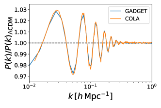
Figure 2: Ratio with respect to the $\Lambda$CDM case of the nonlinear matter power spectra in Fourier space at redshift $z=0$ calculated with the approximate N-body method COLA and with the full N-body code GADGET-3 for the linear oscillations with ${\cal A}_{\rm lin}=0.03$ and $\omega_{\rm lin}=10$ (Ballardini et al. 2020).

We show in Fig. 3 the ratio between the matter power spectrum with primordial oscillations and the one with featureless PPS calculated at redshift $z=0$ for the results both at LO and NLO for the two templates with linear and logarithmic oscillations. We collect in Appendix A the results for different frequencies; see Figs. 7 and 8.

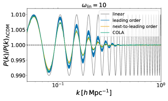
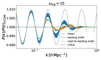
Figure 3: Ratio of IR resummed matter power spectrum at LO (blue) and NLO (orange) obtained for linear (top panel) and logarithmic (bottom panel) oscillations to the one obtained with a power-law PPS at redshift $z=0$ when the frequency $\omega_{\rm X}=10$ and the IR separation scale $k_{\rm S}=\epsilon k$ is varied (with $\epsilon\in[0.3,0.7]$). We also show the results of the linear theory (grey) and the ones obtained from N-body simulations (green).

For the template with undamped linear oscillations, the agreement between N-body simulations and PT results is remarkable for the entire range of frequencies considered, i.e. $\log_{10}\omega_{\rm lin}\in(0.2,\,2)$. At LO, we find differences for the matter power spectrum in Fourier space at redshift $z=0$ less than $1\%$ for $\log_{10}\omega_{\rm lin}>0.6$ and between $1\%$ and $2\%$ for $\log_{10}\omega_{\rm lin}\leq 0.6$. At NLO, we find an agreement better than $1\%$ for all the frequencies and differences $<0.5\%$ for $\log_{10}\omega_{\rm lin}>0.4$. For the template with undamped logarithmic oscillations, we find a similar agreement for the frequencies $\log_{10}\omega_{\rm log}\geq 1$, less than $1\%$ for the LO and less than $0.5\%$ for the NLO. In order to improve the accuracy of the results for low frequencies (see Beutler et al. 2019, for a discussion on the validity of perturbation approach for small frequencies) we can fit a Gaussian damping to the N-body simulation as done by Ballardini et al. (2020).

While we restrict the validation of results to the matter power spectrum in real space, a validation for the halo power spectrum in redshift space has been performed by Chen et al. (2020), showing that current results from PT are able to describe redshift-space clustering observables also in the presence of primordial features.

4.4 Nonlinear reconstruction of primordial features

An alternative to the modelling approach described above is through reconstruction. This takes the opposite logic, by starting from an evolved, nonlinear, matter field where the primordial oscillations have been damped, it tries to recover their undamped states. Reconstruction has long been adopted as a useful technique to undo the effect of structure evolution and retrieve sharper BAO features, hence improving their use as a standard ruler to constrain cosmological parameters (e.g. Eisenstein et al. 2007; Wang et al. 2017; Sarpa et al. 2019), with an even longer history of applications in other subfields of cosmology and astrophysics (e.g. Peebles 1989; Croft & Gaztanaga 1997; Monaco & Efstathiou 1999; Nusser & Branchini 2000; Brenier et al. 2003; Mohayaee et al. 2003; Schmittfull et al. 2017; Zhu et al. 2017; Shi et al. 2018; Birkin et al. 2019; Mao et al. 2021).

From the point of view of reconstruction, there is no fundamental difference between BAO features and features that exist in the primordial density fluctuations on similar length scales: both are present at the time of last scattering, the preservation of both is negatively impacted by late-time cosmic structure formation, and both can be at least partially recovered if such an impact is undone through processes such as reconstruction (e.g. Beutler et al. 2019; Li et al. 2022). Therefore, we expect that reconstruction can find uses in the study of primordial features, at least when the oscillations have similar frequencies as the BAO peaks, e.g. $0.05\lesssim{k}/(h\,{\rm Mpc}^{-1})\lesssim 0.5$ — at scales much larger than this range any significant damping of the features due to cosmological evolution is yet to happen, because structure formation is hierarchical and affects smaller scales first, while on much smaller scales reconstruction becomes unreliable.

Another useful property of reconstruction is that it is possible to include galaxy bias (e.g. Birkin et al. 2019) and RSD (e.g. Monaco & Efstathiou 1999; Burden et al. 2014; Hada & Eisenstein 2018, 2019; Wang et al. 2020) in the pipeline, so that two of the most important theoretical systematic effects in analysing the galaxy redshift power spectrum are taken into account. Of course, caution is due here to ensure that the range of length scales where reconstruction from a catalogue of redshift-space biased tracers can be done reliably covers the range where we hope reconstruction to also benefit the recovery of the primordial features of interest. Checking this naturally requires a more detailed analysis, which may also depend on the reconstruction algorithm in actual use: while a quantitative analysis of this issue is not the topic here, our experience is that the scale range $k\lesssim 0.2\,h\,{\rm Mpc}^{-1}$ or $s\gtrsim 15$–$20\,${\mathrm{\mathnormal{h}}}^{-1}\text{\,}\mathrm{Mpc}$$ satisfies these requirements.

In this work, we exemplify using the nonlinear reconstruction method described in Shi et al. (2018); Birkin et al. (2019); Wang et al. (2020). Other algorithms may give quantitatively different results, though we do not expect a huge variation among the ones that are at an advanced stage of development. The problem of reconstruction can be reduced to identifying a mapping between the initial, Lagrangian coordinate of some particle, $\bm{q}$, and its Eulerian coordinate after evolution, $\bm{x}(t)$, at a later time $t$. If trajectory crossings of particles have not happened, this mapping is unique and can be obtained by solving the mass conservation equation

$$\rho(\bm{x})\,{\rm d}^{3}\bm{x}=\rho(\bm{q})\,{\rm d}^{3}\bm{q}\approx\bar{\rho}\,{\rm d}^{3}\bm{q}\,,$$ (46)

where $\rho(\bm{q})$ and $\rho(\bm{x})$ are, respectively, the initial density field in some infinitesimal volume element ${\rm d}\bm{q}$, and the density field in the same volume element at time $t$, which now has been moved, and possibly deformed, and described by ${\rm d}\bm{x}$. As the density field in the early Universe is homogeneous to a very good approximation, one can take $\rho({\bf q})$ to be a constant, i.e. $\rho(\bm{q})\simeq\bar{\rho}$.

We define the displacement field $\bm{\Psi}$ between the final and initial positions of a particle as $\bm{\Psi}(\bm{x})=\bm{x}-\bm{q}$, which can be rewritten as

$$\bm{\nabla}_{\bm{x}}{\Theta}(\bm{x})\equiv\bm{q}=\bm{x}-\bm{\Psi}(\bm{x})\,,$$ (47)

with $\Theta({\bf x})$ being the displacement potential. Here we have assumed the displacement field to be curl-free, i.e. $\bm{\nabla}\times\bm{\Psi}=\bm{0}$, which is valid only on large scales. Combining Eq. (47) and Eq. (46) gives

$$\det[\nabla^{i}\nabla_{j}\Theta({\bf x})]=\frac{\rho({\bf x})}{\bar{\rho}}\equiv 1+\delta({\bf x})\,,$$ (48)

where $\delta(\bm{x})=\rho(\bm{x})/\bar{\rho}-1$ is the density contrast at time $t$, ‘${\det}$’ is the determinant of a matrix, here the Hessian of $\Theta({\bf x})$, and $i,j=1,2,3$. Shi et al. (2018) proposed to solve this equation as a nonlinear partial differential equation with cubic power of second-order derivatives of $\Theta$. This was later extended by Birkin et al. (2019) to cases where $\delta(\bm{x})$ in the above can be the density contrast of some biased tracers of the dark matter field, such as galaxies and dark matter haloes.

Once $\Theta(\bm{x})$ is solved, one can obtain $\bm{\Psi}(\bm{x})$ and the reconstructed density field is given by

$$\delta_{\rm r}=-\nabla_{\bm{q}}\cdot\bm{\Psi}(\bm{q})\,,$$ (49)

where we express ${\bf\Psi}$ in terms of the Lagrangian coordinate $\bm{q}$, since the divergence $\nabla_{\bm{q}}$ therein is with respect to $\bm{q}$. This calculation means that we need to have $\bm{\Psi}(\bm{q})$ on a regular $\bm{q}$-grid, which can be done using, e.g. the Delaunay Tessellation Field Estimator code (DTFE; Schaap & van de Weygaert 2000; van de Weygaert & Schaap 2009; Cautun & van de Weygaert 2011), by interpolating $\bm{\Psi}(\bm{x})$ to the target $\bm{q}$-grid.

The quantity $\delta_{\rm r}$ obtained above is an approximation to the initial linear matter density contrast, linearly extrapolated to time $t$ (bearing in mind that all the discussion in this subsection is for $\Lambda$CDM, for which the linear growth factor is scale-independent). As a result, part of the structure-formation-induced damping of the BAO or primordial features imprinted in the density field can be undone this way.

The damping of the BAO or primordial wiggles can be described by a Gaussian fitting function (cf. Sect. 4.3; e.g. Vasudevan et al. 2019; Beutler et al. 2019; Ballardini et al. 2020), effectively multiplying the undamped power spectrum wiggles $O_{\rm w}^{\rm undamped}$ by a Gaussian function

$${O}_{\rm w}^{\rm damped}(k,z)={O}_{\rm w}^{\rm undamped}(k,z)\exp\left[-\frac{k^{2}\zeta(z)^{2}}{2}\right]\,,$$ (50)

where $\zeta(z)$ is the parameter quantifying the level of damping. In the linearly-evolved density field with no damping, one has $\zeta=0$. For the evolved nonlinear matter or galaxy field, $\zeta>0$ with its values depending on redshift, tracer type, tracer number density etc., and the reconstructed density field generally features a smaller yet positive value of $\zeta$.

We generate a suite of N-body simulations using the initial conditions described in Sect. 4.3, which includes a no-wiggle model and 20 wiggled models. The simulations are performed using the parallel N-body code ramses (Teyssier 2002). We output 4 snapshots of the DM respectively at $z=1.5$, $1.0$, $0.5$ and $0$, and measure the matter power spectrum of each of the snapshots. We follow the same reconstruction pipeline employed in Li et al. (2022) to reconstruct the density fields from each of the snapshots for all the models (shown in Fig. 9). We have also performed reconstruction from halo catalogues, though the results are noisier and not shown here; the DM reconstruction result can be considered as an ideal scenario, which serves as a limit of what can be achieved from halo or galaxy reconstruction with increasing tracer number density. We will present the reconstruction from mock galaxy catalogues in redshift space based on the same set of simulations in a separate work. Fig. 9 shows that reconstruction can help recover the weakened wiggles down to $k\simeq 1\,h\,{\rm Mpc}^{-1}$. Note that, in order to avoid artificial features in the $P(k)$ of the models with high-frequency wiggles, we have binned $P(k)$ in $k$ bins of width $0.001\,h\,{\rm Mpc}^{-1}$.

To estimate the best-fit values of $\zeta(z)$, the Gaussian function is applied to fit the envelopes of the unreconstructed and reconstructed wiggled spectra, $O_{\rm w}^{\rm damped}(k,z)$. We apply the Hilbert transform to measure the wiggle envelopes for each wiggled model and each redshift. Nevertheless, we expect that the damping parameter $\zeta(z)$, for both the unreconstructed and the reconstructed cases, should mostly depend on the nonlinear structure formation and be insensitive to the wiggle model, given that the wiggles are weak. We have explicitly checked this by comparing the envelopes of $O^{\rm damped}_{\rm w}$ and $O^{\rm undamped}_{\rm w}$ of the different models, and finding them to agree very well. As a result, to get $\zeta(z)$, the $O_{\rm w}$ envelopes of all wiggle models at redshift $z$ could be combined to do a single least-squares fitting. In practice, because the measurement of the envelopes is not very reliable for the low-frequency featured models due to the very few wiggles in the $k$ range of fitting, $k=(0.05$–$1)\,h\,\rm Mpc^{-1}$, we select only the 10 high-frequency feature models to fit $\zeta(z)$, and the result is given in Table 1. We nevertheless have checked that the fitted envelope also well describes the wiggles of low-frequency models.

Table 1: Best-fit values of $\zeta(z)$ for unreconstructed (reconstructed) wiggle spectra. Columns respectively denote (1) redshift, (2) unreconstructed wiggles, (3) reconstructed wiggles, and (4) reconstruction efficiency (defined as $\zeta_{\rm unrec}/\zeta_{\rm rec}$).

$z$	${\rm unrec}$	${\rm rec}$	${\rm efficiency}$
$0.0$	$8.16$	$2.04$	$4.00$
$0.5$	$6.49$	$1.69$	$3.84$
$1.0$	$5.23$	$1.41$	$3.71$
$1.5$	$4.32$	$1.21$	$3.57$

5 Expected constraints from Euclid primary probes

In this section, we show the results of the Fisher analysis for the cosmological parameters of interest corresponding to a flat $\Lambda$CDM,

$$\Theta_{\rm final}=\left\{\Omega_{\rm m,0},\Omega_{\rm b,0},h,n_{\rm s},\sigma_{8},{\cal A}_{X},\omega_{X},\phi_{X}\right\}\,,$$ (51)

after marginalisation over spectroscopic and photometric nuisance parameters. We compute the spectroscopic galaxy clustering (GC_sp), the photometric galaxy clustering (GC_ph), the weak lensing (WL), and the cross-correlation between the two photometric probes (XC) in two configurations: a pessimistic setting and an optimistic one. For the pessimistic setting, for GC_sp we have $k_{\rm max}=0.25\,h\,{\rm Mpc}^{-1}$, for GC_ph and XC we have $\ell_{\rm max}=750$, and for WL we have $\ell_{\rm max}=1500$. In addition, we impose a cut in redshift of $z<0.9$ to GC_ph to limit any possible cross-correlation between spectroscopic and photometric data. For the optimistic setting, we extend GC_sp to $k_{\rm max}=0.30\,h\,{\rm Mpc}^{-1}$, GC_ph and XC to $\ell_{\rm max}=3000$, and WL to $\ell_{\rm max}=5000$, without imposing any redshift cut to GC_ph.

Table 2: Fisher-forecast 68.3% CL marginalised uncertainties on cosmological and primordial feature parameters, relative to their corresponding fiducial values, for LIN and LOG in the pessimistic and optimistic settings, using Euclid observations GC_sp, WL+GC_ph+XC, and their combination.

jonquil     LIN    $\omega_{\rm lin}=10$
	$\Omega_{\rm m,0}$	$\Omega_{\rm b,0}$	$h$	$n_{\rm s}$	$\sigma_{8}$	${\cal A}_{\rm lin}$	$\omega_{\rm lin}$	$\phi_{\rm lin}$
lavender(web)    Pessimistic setting
GCsp $(k_{\rm max}=0.25\,h\,{\rm Mpc}^{-1})$	1.5%	2.1%	0.34%	1.2%	0.78%	23%	4.1%	0.11
WL+GCph+XC	0.83%	5.7%	4.0%	1.6%	0.39%	32%	5.7%	0.12
GCsp+WL+GCph+XC($z<0.9$)	0.64%	1.3%	0.11%	0.59%	0.29%	21%	2.9%	0.083
lavender(web)    Optimistic setting
GCsp  $(k_{\rm max}=0.3\,h\,{\rm Mpc}^{-1})$	1.3%	1.8%	0.27%	1.1%	0.71%	23%	3.6%	0.10
WL+GCph+XC	0.27%	4.4%	2.5%	0.66%	0.13%	31%	2.8%	0.072
GCsp+WL+GCph+XC	0.24%	1.1%	0.095%	0.22%	0.11%	18%	1.2%	0.047
jonquil     LOG    $\omega_{\rm log}=10$
	$\Omega_{\rm m,0}$	$\Omega_{\rm b,0}$	$h$	$n_{\rm s}$	$\sigma_{8}$	${\cal A}_{\rm log}$	$\omega_{\rm log}$	$\phi_{\rm log}$
lavender(web)    Pessimistic setting
GCsp $(k_{\rm max}=0.25\,h\,{\rm Mpc}^{-1})$	1.4%	2.2%	0.34%	1.2%	0.77%	25%	4.7%	0.053
WL+GCph+XC	0.83%	5.7%	4.0%	1.6%	0.38%	32%	5.7%	0.12
GCsp+WL+GCph+XC($z<0.9$)	0.64%	1.4%	0.11%	0.60%	0.29%	22%	2.4%	0.044
lavender(web)    Optimistic setting
GCsp  $(k_{\rm max}=0.3\,h\,{\rm Mpc}^{-1})$	1.3%	2.0%	0.27%	1.1%	0.71%	25%	4.7%	0.052
WL+GCph+XC	0.27%	4.4%	2.5%	0.66%	0.13%	31%	2.8%	0.072
GCsp+WL+GCph+XC	0.24%	1.1%	0.096%	0.22%	0.11%	18%	1.1%	0.035

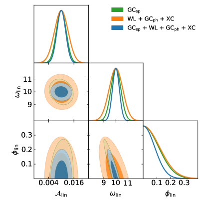
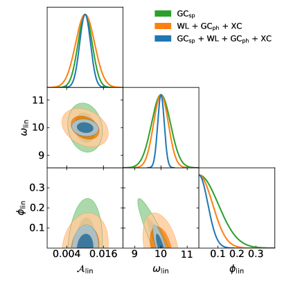
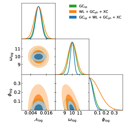
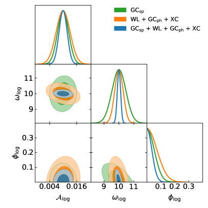
Figure 4: Fisher-forecast marginalised two-dimensional contours and one-dimensional probability distribution functions from Euclid on the primordial feature parameters for the LIN model with $\omega_{\rm lin}=10$ (top panels) and the LOG model with $\omega_{\rm log}=10$ (bottom panels). Left (right) panels correspond to the pessimistic (optimistic) setting for GC_sp (green), WL+GC_ph+XC (orange), and their combination (blue).

We start by presenting results for a fiducial scenario with ${\cal A}_{\rm X}=0.01$, $\omega_{\rm X}=10$, and $\phi_{\rm X}=0$. The marginalised uncertainties on the cosmological parameters and primordial feature parameters, percentages relative to the corresponding fiducial values, are collected in Table 5 for the pessimistic (top panel) and optimistic (bottom panel) settings. The marginalised 68.3% and 95.5% confidence level (CL) contours for the primordial feature parameters are shown in Fig. 4. For the fiducial value parameters, uncertainties on the amplitude of the primordial feature oscillations are dominated by GC_sp measurements resulting in ${\cal A}_{\rm lin}=0.0100\pm 0.0023$ ($\pm 0.0023$) and ${\cal A}_{\rm log}=0.0100\pm 0.0025$ ($\pm 0.0025$) at 68.3% CL for the pessimistic (optimistic) setting. Combining GC_sp with the combination of photometric information, i.e. WL+GC_ph+XC, we find ${\cal A}_{\rm lin}=0.0100\pm 0.0021$ ($\pm 0.0018$) and ${\cal A}_{\rm log}=0.0100\pm 0.0022$ ($\pm 0.0018$) at 68.3% CL for the pessimistic (optimistic) setting.

For GC_sp, bounds on the primordial amplitude parameter ${\cal A}_{X}$ strongly depend on the primordial frequency value $\omega_{X}$; see Huang et al. (2012); Ballardini et al. (2016); Slosar et al. (2019); Beutler et al. (2019); Ballardini et al. (2020). Low frequencies, lower than the BAO one, leave a broad modification on the matter power spectrum and are expected to be better constrained by CMB measurements. On the other hand, the imprint from high-frequency primordial oscillations is smoothed by projection effects on the observed matter power spectrum. Moreover, for the linear model the uncertainties for frequencies around the BAO frequency, i.e. $\log_{10}\omega_{\rm lin}\sim 0.87$, are degraded. For the combination of photometric probes, bounds on the primordial amplitude parameter ${\cal A}_{X}$ are smoothed by projection effects in angular space and high-frequency primordial oscillations are severely washed out on the observed matter power spectrum. On the other hand, uncertainties for frequencies around the BAO scale and lower frequencies are tighter compared to the results from GC_sp. This represents an important result considering the lower accuracy of the PT predictions for low frequencies.

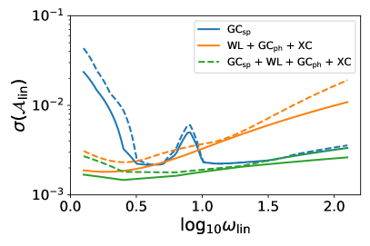
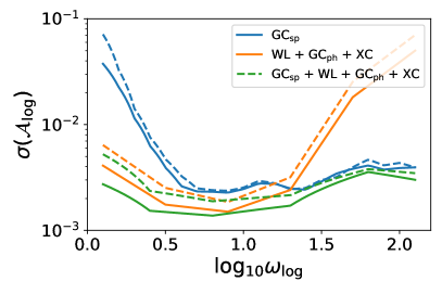
Figure 5: Marginalised uncertainties on ${\cal A}_{X}$ as a function of the primordial frequency $\omega_{X}$ for the LIN model (top panel) and the LOG model (bottom panel). We show uncertainties for GC_sp (blue), WL+GC_ph+XC (orange), and their combination (green). Dashed (solid) curves correspond to the pessimistic (optimistic) setting.

In Fig. 5, we show the uncertainties at 68.3% CL for different values of the primordial frequency $\log_{10}\omega_{\rm X}$ within the range $(0.1,\,2.1)$. The combination of the spectroscopic and photometric probes allows us to reach uncertainties of 0.002–0.003 on the primordial feature amplitude for the entire range of frequencies.

The nonlinear reconstruction described in Sect. 4.4 applied to GC_sp reduces significantly the uncertainties on the feature amplitude, going from $\sigma({\cal A}_{\rm lin})=0.0023$ ($0.0023$) at 68.3% CL for the pessimistic (optimistic) setting to $\sigma({\cal A}_{\rm lin})=0.0014$ ($0.0013$), and going from $\sigma({\cal A}_{\rm log})=0.0025$ ($0.0025$) to $\sigma({\cal A}_{\rm log})=0.0016$ ($0.0012$). Combining with the photometric probes, we find $\sigma({\cal A}_{\rm lin})=0.0014$ ($0.0012$) at 68.3% CL and $\sigma({\cal A}_{\rm log})=0.0015$ ($0.0012$) for the pessimistic (optimistic) setting, compared with $\sigma({\cal A}_{\rm lin})=0.0021$ ($0.0018$) at 68.3% CL and $\sigma({\cal A}_{\rm log})=0.0022$ ($0.0018$) for the same settings without reconstruction. We also note that in the analysis here $k_{\rm max}$ is set to be $0.25$–$0.30\leavevmode\nobreak\ h\leavevmode\nobreak\ {\rm Mpc}^{-1}$, while in Li et al. (2022) $k_{\rm max}=0.50\leavevmode\nobreak\ h\leavevmode\nobreak\ {\rm Mpc}^{-1}$ is used.

6 Power spectrum and bispectrum combination

In this section, we present the forecast results on primordial features by combining the power spectrum and bispectrum signals. The presence of a sharp feature in the inflaton potential violates the slow-roll evolution, generating a linearly spaced oscillating primordial bispectrum. In this case the primordial bispectrum can be characterised by the standard amplitude parameter $f_{\rm NL}^{\rm lin}$, the phase $\phi_{\rm lin}^{B}$, and the frequency $\omega_{\rm lin}$, and it is given by (Chen et al. 2007, 2008)

$$B_{\Phi}^{\rm lin}(k_{1},k_{2},k_{3})=f_{\rm NL}^{\rm lin}\frac{6A^{2}}{k_{1}^{2}k_{2}^{2}k_{3}^{2}}\sin\left[\omega_{\rm lin}\frac{K}{k_{*}}+2\pi\phi_{\rm lin}^{B}\right]\,,$$ (52)

where $K=k_{1}+k_{2}+k_{3}$ and $A=9/25(2\pi^{2})k_{*}^{1-n_{\rm s}}A_{\rm s}$ is the normalisation parameter of $P_{\Phi}=A/k^{(4-n_{\rm s})}$.

A periodically modulated inflaton potential leads to resonances in the inflationary fluctuations with logarithmically-spaced oscillations (Chen et al. 2008). This generates oscillatory features in the primordial power spectrum (see Sect. 4) and bispectrum (Flauger et al. 2010; Hannestad et al. 2010; Barnaby et al. 2012). In this case, the primordial bispectrum is given by (Chen 2010)

$$B_{\Phi}^{\rm log}(k_{1},k_{2},k_{3})=f_{\rm NL}^{\rm log}\frac{6A^{2}}{k_{1}^{2}k_{2}^{2}k_{3}^{2}}\sin\left[\omega_{\rm log}\ln\left(\frac{K}{k_{*}}\right)+2\pi\phi_{\rm log}^{B}\right]\,,$$ (53)

where $\phi_{\rm log}^{B}$ and $f_{\rm NL}^{\rm log}$ are the phase and the amplitude, respectively, of the generated logarithmic features on the primordial bispectrum. Note that here we assume the frequency of the primordial feature bispectrum to be the same as in the case of the power spectrum (see Sect. 4.1)

The redshift space model, for the galaxy bispectrum, is given after considering non-Gaussian initial conditions, as dictated by the oscillatory features, up to second order terms in RSD, bias, and matter expansions. The tree-level modelling can be written as

$$P_{g}(\bm{k},z)=D^{P}(\bm{k},z)Z_{1}^{2}(\bm{k},z)P^{\rm lin}(k,z)+P_{\varepsilon}(z)\,,$$ (54)

$$B_{g}(\bm{k}_{1},\bm{k}_{2},\bm{k}_{3},z)=D^{B}(\bm{k}_{1},\bm{k}_{2},\bm{k}_{3},z)$$

$$\times\bigg{[}Z_{1}(\bm{k}_{1},z)Z_{1}(\bm{k}_{2},z)Z_{1}(\bm{k}_{3},z)B_{I}(\bm{k}_{1},\bm{k}_{2},\bm{k}_{3},z)$$

$$+2Z_{1}(\bm{k}_{1},z)Z_{1}(\bm{k}_{2},z)Z_{2}(\bm{k}_{1},\bm{k}_{2},z)P_{\rm lin}(k_{1},z)P_{\rm lin}(k_{2},z)+2\text{ perm}\bigg{]}$$

$$+2P_{\varepsilon\varepsilon_{\delta}}\big{[}Z_{1}(\bm{k}_{1},z)P_{\rm lin}(k_{1},z)+2\text{ perm}\big{]}+B_{\varepsilon}\,,$$ (55)

where the linearly propagated primordial oscillatory bispectrum is

$$B_{I}(\bm{k}_{1},\bm{k}_{2},\bm{k}_{3},z)=M(k_{1},z)M(k_{2},z)M(k_{3},z)B_{\Phi}^{X}(k_{1},k_{2},k_{3},z)$$ (56)

with $B_{\Phi}^{X}$ given by Eqs. (52) and (53) for the linear and logarithmic oscillations, respectively. The redshift space kernels are given by

$$Z_{1}(\bm{k}_{i},z)=b_{1}(z)+f\mu_{i}^{2}\,,$$ (57)

$$Z_{2}(\bm{k}_{i},\bm{k}_{j},z)=b_{1}(z)F_{2}(\bm{k}_{i},\bm{k}_{j})+f(z)\mu_{ij}^{2}G_{2}(\bm{k}_{i},\bm{k}_{j})+\frac{b_{2}(z)}{2}$$

$$+\frac{b_{s^{2}}(z)}{2}S_{2}(\bm{k}_{i},\bm{k}_{j})+\frac{f(z)\mu_{ij}k_{ij}}{2}\left[\frac{\mu_{i}}{k_{i}}Z_{1}(\bm{k}_{j},z)+\frac{\mu_{j}}{k_{j}}Z_{1}(\bm{k}_{i},z)\right]\,,$$ (58)

where $\mu_{i}=\bm{k}_{i}\cdot\hat{z}/k_{i}$ is the cosine of the angle between the wave vector $\bm{k}_{i}$ and the line of sight, $\mu=\mu_{1}+\ldots\mu_{n}$, and $k=|\bm{k}_{1}+\ldots\bm{k}_{n}|$. Specifically $\mu_{12}=(\mu_{1}k_{1}+\mu_{2}k_{2})/k_{12}$ and $k_{12}^{2}=(\bm{k}_{1}+\bm{k}_{2})^{2}$. The kernels $F_{2}(\bm{k}_{i},\bm{k}_{j})$ and $G_{2}(\bm{k}_{i},\bm{k}_{j})$ are the second-order symmetric PT kernels (Bernardeau et al. 2002), while $S_{2}(\bm{k}_{1},\bm{k}_{2})=(\bm{k}_{1}\cdot\bm{k}_{2})^{2}/(k_{1}^{2}k_{2}^{2})-1/3$ is the tidal kernel (McDonald & Roy 2009; Baldauf et al. 2012). The second-order tidal field bias term, following the convention of (Baldauf et al. 2012), is given by $b_{s^{2}}(z)=-4[b_{1}(z)-1]/7$. The redshift-space bispectrum is characterised by five variables: three to define the triangle shape (e.g. the sides $k_{1}$, $k_{2}$, $k_{3}$) and two that characterise the orientation of the triangle relative to the line of sight, i.e. $B_{\rm g}(\bm{k}_{1},\bm{k}_{2},\bm{k}_{3},z)=B_{\rm g}(k_{1},k_{2},k_{3},\mu_{1},\phi,z)$. The forecasts presented here use the information of the bispectrum monopole obtained after taking the average over all angles.

Note that the presence of an oscillatory primordial bispectrum generates a scale-dependent correction to the linear bias, in a similar manner to the local primordial non-Gaussian case (see e.g. Karagiannis et al. 2018, for discussions). Cabass et al. (2018) show that the scale-dependent correction oscillates with scale with an envelope similar to that of equilateral primordial non-Gaussianity (PNG) (see e.g. Schmidt & Kamionkowski 2010; Scoccimarro et al. 2012; Schmid & Hui 2013; Assassi et al. 2015, for a discussion), while their findings indicate that the amplitude of such a term is very small to be detected by upcoming surveys. Therefore, we do not consider the scale-dependent terms in our analysis and exclude them from the expressions of the redshift kernels presented above. This means that the degeneracy between the scale-dependent bias coefficient and the primordial bispectrum amplitude ($f_{\rm NL}^{\rm X}$), shown in Barreira (2020), does not affect our forecasts.

The multiplicative factors $D^{P}(\bm{k},z)$ and $D^{B}(\bm{k}_{1},\bm{k}_{2},\bm{k}_{3},z)$, which incorporate errors on redshift measurements and FOG effect, are $D^{P}(\bm{k},z)=\exp[-k\mu(\sigma_{\rm p}^{2}(z)+\sigma_{\rm r}^{2}(z))]$ and $D^{B}(\bm{k}_{1},\bm{k}_{2},\bm{k}_{3},z)=\exp[-(k_{1}^{2}\mu_{1}^{2}+k_{2}^{2}\mu_{2}^{2}+k_{3}^{2}\mu_{3}^{2})(\sigma_{\rm p}^{2}(z)+\sigma_{\rm r}^{2}(z))/2]$ for the power spectrum and bispectrum, respectively (see Sect. 3.1 for details). The fiducial values of the stochastic terms in Eqs. (54) and (55) are taken to be those predicted by Poisson statistics (Schmidt 2016; Desjacques et al. 2018), i.e. $P_{\varepsilon}=1/\bar{n}_{\rm g}$, $P_{\varepsilon\varepsilon_{\delta}}=b_{1}/(2\bar{n}_{\rm g})$, and $B_{\varepsilon}=1/\bar{n}_{\rm g}^{2}$.

The AP effect is taken into account also for the bispectrum similar to the power spectrum case (see Sect. 3.1). The observed bispectrum is thus given by (see e.g. Karagiannis et al. 2022)

$$B^{\rm obs}_{\rm g}(k_{{\rm ref,}1} ,k_{{\rm ref,}2},k_{{\rm ref,}3},\mu_{{\rm ref,}1},\phi;z)$$

$$=\frac{1}{q_{\parallel}^{2}q_{\perp}^{4}}B_{\rm g}\left(k(k_{{\rm ref,}1}),k(k_{{\rm ref,}2}),k(k_{{\rm ref,}3}),\mu(\mu_{{\rm ref,}1}),\phi;z\right)\,.$$ (59)

Here we again use the Fisher matrix formalism to produce forecasts on the model parameters that control the primordial oscillations. The Fisher matrix of the redshift galaxy power spectrum is given by Eq. (12), while for the bispectrum the Fisher matrix for one redshift bin $z_{i}$ is given by

$$F_{\alpha\beta}^{B}(z_{i}) =\frac{1}{4\pi}\!\sum_{k_{1},k_{2},k_{3}}\!\int_{-1}^{1}\!\!{\rm d}\mu_{1}\!\!\int_{0}^{2\pi}\!\!{\rm d}\phi\frac{1}{\Delta B^{2}(\bm{k}_{1},\bm{k}_{2},\bm{k}_{3},z_{i})}$$

$$\times\frac{\partial B_{\rm g}^{\rm obs}(\bm{k}_{1},\bm{k}_{2},\bm{k}_{3},z_{i})}{\partial p_{\alpha}}\frac{\partial B_{\rm g}^{\rm obs}(\bm{k}_{1},\bm{k}_{2},\bm{k}_{3},z_{i})}{\partial p_{\beta}}\,,$$ (60)

where the sum over triangles has $k_{\rm min}\leq k_{3}\leq k_{2}\leq k_{1}\leq k_{\rm max}$, and $k_{1}$, $k_{2}$ and $k_{3}$ satisfy the triangle inequality. The bin size $\Delta k$ is taken to be the fundamental frequency of the survey, $k_{\rm f}=2\pi/L$, where for simplicity we approximate the survey volume as a cube, $L=V_{\rm survey}^{1/3}$. The $k$ mode is binned with a bin size of $\Delta k$, and here we consider $\Delta k=k_{\rm f}$, between its minimum and maximum values $k_{\rm min}=k_{\rm f}$ and $k_{\rm max}$. Gaussian approximation is used for the covariance of bispectrum, i.e. the off-diagonal terms are considered to be zero. The variance for the bispectrum is then (Sefusatti et al. 2007)

$$\Delta B^{2}(\bm{k}_{1},\bm{k}_{2},\bm{k}_{3},z)=s_{123}\,\pi\,k_{\rm f}(z)^{3}\,\frac{P_{\rm g}(\bm{k}_{1},z)\,P_{\rm g}(\bm{k}_{2},z)\,P_{\rm g}(\bm{k}_{3},z)}{k_{1}k_{2}k_{3}\,\Delta k(z)^{3}}\,,$$ (61)

where $s_{123}=6,2,1$ for equilateral, isosceles, and non-isosceles triangles, respectively. In addition, for degenerate configurations, i.e. $k_{i}=k_{j}+k_{m}$, the bispectrum variance should be multiplied by a factor of 2 (Chan & Blot 2017; Desjacques et al. 2018). We use the Fisher matrix of Eq. (6) to generate bispectrum forecasts on the parameters of interest

$$\Theta_{\rm final}^{B}=\left\{\Omega_{\rm m,0},\Omega_{\rm b,0},h,n_{\rm s},\sigma_{8},A_{X},\omega_{X},\phi_{X},f_{\rm NL}^{X},\phi_{X}^{B}\right\}\,.$$ (62)

The initial parameter vector considers all the parameters of the bispectrum tree-level modelling (i.e. cosmological parameters, biases, AP parameters, growth rate, and FOG amplitudes) to be free, and after marginalisation we derive the constraints for $\Theta_{\rm final}^{B}$. The forecasted marginalised $1\sigma$ errors on the feature model parameters, coming from the spectroscopic galaxy clustering, are presented in Table 3.

The galaxy bispectrum is capable of providing constraints not only on the feature parameters related to the primordial bispectrum but also on those controlling the primordial power spectrum feature model. The latter is due to the $P_{\rm lin}(k_{i})P_{\rm lin}(k_{j})$ terms that are present at tree level in the galaxy bispectrum (55) and can provide constraints equivalent to or even better than the galaxy power spectrum, especially in the case of a high $k_{\rm max}$. This can be seen in Table 3, where adding the power spectrum to the bispectrum improves the forecasts by a few percent. This highlights the importance of a bispectrum analysis for the type of feature models discussed in this work. On the other hand, the sole contribution to the constraints on the $f_{\rm NL}^{\rm X}$ and $\phi^{B}_{X}$ feature parameters is the primordial component $B_{I}$ of the galaxy bispectrum, justifying the less rigorous forecasts presented here.

Table 3: Forecasted marginalised uncertainties at 68.3% CL from the Fisher-matrix analysis on the feature model parameters in the case of linear and logarithmic oscillations, by using the Euclid GC_spbispectrum and the joint power spectrum+bispectrum signal, for the pessimistic and optimistic settings.

P B P+B Pessimistic setting ($k_{\rm max}=0.25\,h\,{\rm Mpc}^{-1}$) $A_{\rm lin}$ 23% 16% 13% $\omega_{\rm lin}$ 4.1% 2.1% 1.7% $\phi_{\rm lin}$ 0.11 - 0.049 $f_{\rm NL}^{\rm lin}$ - 31 31 $\phi_{\rm lin}^{B}$ - 4.9 4.9 $A_{\rm log}$ 25% 17% 13% $\omega_{\rm log}$ 4.7% 2.9% 2.4% $\phi_{\rm log}$ 0.053 - 0.026 $f_{\rm NL}^{\rm log}$ - 33 32 $\phi_{\rm log}^{B}$ - 5.2 5.1 Optimistic setting ($k_{\rm max}=0.3\,h\,{\rm Mpc}^{-1}$) $A_{\rm lin}$ 23% 12% 11% $\omega_{\rm lin}$ 3.6% 1.4% 1.2% $\phi_{\rm lin}^{P}$ 0.10 - 0.039 $f_{\rm NL}^{\rm lin}$ - 29 29 $\phi_{\rm lin}^{B}$ - 4.6 4.6 $A_{\rm log}$ 25% 13% 11% $\omega_{\rm log}$ 4.7% 2.2% 2.0% $\phi_{\rm log}$ 0.052 - 0.023 $f_{\rm NL}^{\rm log}$ - 30 30 $\phi_{\rm log}^{B}$ - 4.8 4.8

7 Combination with CMB data

Future CMB polarisation data from ground-based experiments, such as Simons Observatory (Ade et al. 2019) and CMB-S4 (Abazajian et al. 2019), and satellites, such as LiteBIRD (LiteBIRD Collaboration: Allys et al. 2023), will be able to reduce the uncertainties on the PPS, in particular in the presence of oscillatory signals. Indeed, E-mode polarisation is sourced by velocity gradient (scattering only) leading to sharper transfer functions compared to the temperature ones helping to characterise primordial features in the PPS; see Mortonson et al. (2009); Miranda et al. (2015); Ballardini et al. (2016); Finelli et al. (2018); Hazra et al. (2018).

We consider the information available in the CMB data by using power spectra from temperature, E-mode polarisation, and CMB lensing in combination with Euclid observations. We do not consider B-mode polarisation since it does not add information for the specific models examined here. We also neglect the cross-spectra between CMB fields and Euclid primary probes; see Euclid Collaboration: Ilić et al. (2022) for a complete characterisation and quantification of the importance of cross-correlation between CMB and Euclid measurements. Following Euclid Collaboration: Ilić et al. (2022), we consider three CMB experiments: Planck-like, Simons Observatory (SO), and CMB-S4. Noise curves correspond to isotropic noise deconvolved with instrumental beam (Knox 1995)

$${\cal N}_{\ell}^{X}=w_{X}^{-1}b_{\ell}^{-2}\,,\qquad b_{\ell}=\exp\left[-\ell(\ell+1)\theta_{\rm FWHM}^{2}/(16\ln 2)\right]\,,$$ (63)

where $\theta_{\rm FWHM}$ is the full-width-at-half-maximum (FWHM) of the beam, $w_{T}$ and $w_{E}$ are the inverse square of the detector noise levels for temperature and polarisation, respectively. CMB lensing noise is reconstructed through minimum-variance estimator for the lensing potential using quicklens code; see Okamoto & Hu (2003).

For the Planck-like experiment, we use an effective sensitivity in order to reproduce the Planck 2018 results for the $\Lambda$CDM model (Planck Collaboration: Aghanim et al. 2020b) avoiding the complexity of the real-data likelihood (Planck Collaboration: Aghanim et al. 2020c). We use noise specifications corresponding to in-flight performances of the $143\,{\rm GHz}$ channel of the high-frequency instrument (HFI) (Planck Collaboration: Aghanim et al. 2020a) with a sky fraction $f_{\rm sky}=0.7$ and a multipole range for temperature and polarisation from $\ell_{\rm min}=2$ to $\ell_{\rm max}=1500$. The E-mode polarisation noise is inflated by a factor of 8 to reproduce the uncertainty of the optical depth parameter $\tau$; see Bermejo-Climent et al. (2021). Finally, CMB lensing is obtained by combining the $143\,{\rm GHz}$ and $217\,{\rm GHz}$ HFI channels assuming a conservative multipole range of 8–400. For the CMB, we also consider the optical depth at reionization $\tau$ and then we marginalise over it before combining the CMB Fisher matrix with the Euclid ones.

For the SO-like experiment, we use noise curves provided by the SO collaboration in Ade et al. (2019) taking into account residuals and noises from component separation. We use spectra from $\ell_{\rm min}=40$ to $\ell_{\rm max}=3000$ for temperature and temperature-polarisation cross-correlation, and $\ell_{\rm max}=5000$ for E-mode polarisation. CMB lensing and temperature-lensing cross-correlation spectra cover the multipole range of 2–3000. The sky fraction considered is $f_{\rm sky}=0.4$. We complement the SO-like information with the Planck-like large-scale data in the multipole range of 2–40 in both temperature and polarisation.

For CMB-S4, we use noise sensitivities of $1\,\mu{\rm K}\,{\rm arcmin}$ in temperature and $\sqrt{2}\,\mu{\rm K}\,{\rm arcmin}$ in polarisation, with resolution of $\theta_{\rm FWHM}=1\,{\rm arcmin}$. We assume data over the same multipole ranges of SO and with the same sky coverage.

Table 4: Fisher-matrix-based forecasted 68.3% CL marginalised uncertainties on the feature model parameters, relative to their corresponding fiducial values (${\cal A}_{\rm X}=0.01$, $\omega_{\rm X}=10$, $\phi_{\rm X}=0$), for LIN and LOG in the pessimistic and optimistic settings, using Euclid (GC_sp+WL+GC_ph+XC) in combination with the CMB.

	Euclid	Euclid	Euclid
	+ Planck-like	+ SO-like	+ CMB-S4
		+ Planck low-$\ell$	+ Planck low-$\ell$
Pessimistic setting
$A_{\rm lin}$	18%	14%	12%
$\omega_{\rm lin}$	2.4%	1.2%	1.0%
$\phi_{\rm lin}$	0.066	0.046	0.043
$A_{\rm log}$	17%	11%	7.9%
$\omega_{\rm log}$	1.9%	1.6%	1.5%
$\phi_{\rm log}$	0.048	0.036	0.033
Optimistic setting
$A_{\rm lin}$	16%	13%	12%
$\omega_{\rm lin}$	1.0%	0.92%	0.85%
$\phi_{\rm lin}$	0.042	0.038	0.037
$A_{\rm log}$	15%	10%	7.6%
$\omega_{\rm log}$	1.1%	1.0%	0.98%
$\phi_{\rm log}$	0.037	0.027	0.024

In Table 4, we show the marginalised uncertainties on the primordial feature parameters, percentage relative to the corresponding fiducial values, for the optimistic and pessimistic Euclid + CMB combination. Uncertainties on the primordial feature amplitude improve by 15%–50% depending on the choice of Euclid settings and on the CMB experiment considered, for a frequency value of $\omega_{\rm X}=10$.

8 Conclusions

We have explored the constraining power of the future Euclid space mission for oscillatory primordial features in the primordial power spectrum (PPS) of density perturbations. We have considered two templates with undamped oscillations, i.e. with constant amplitude all over the PPS, one linearly and one logarithmically spaced in $k$-space. We have used a common baseline set of parameters for both the templates with amplitude ${\cal A}_{\rm X}=0.01$, frequency $\omega_{\rm X}=10$, and phase $\phi_{\rm X}=0$, where X = {lin, log}.

Following previous studies for $\Lambda$CDM and simple extensions in Euclid Collaboration: Blanchard et al. (2020), we have calculated Fisher-matrix-based uncertainties from Euclid primary probes, i.e. spectroscopic galaxy clustering (GC_sp) and the combination of photometric galaxy clustering (GC_ph) and photometric weak lensing (WL); see Sect. 3. We have considered two sets of Euclid specifications: a pessimistic setting with $k_{\rm max}=0.25\,h\,{\rm Mpc}^{-1}$ for GC_sp, $\ell_{\rm max}=1500$ for WL, $\ell_{\rm max}=750$ for GC_ph and XC, and a cut in redshift of $z<0.9$ to GC_ph; an optimistic setting with $k_{\rm max}=0.30\,h\,{\rm Mpc}^{-1}$ for GC_sp, $\ell_{\rm max}=5000$ for WL, and $\ell_{\rm max}=3000$ for GC_ph and XC.

We have modelled the nonlinear matter power spectrum with time-sliced perturbation theory predictions at leading order (Vasudevan et al. 2019; Beutler et al. 2019; Ballardini et al. 2020; Ballardini & Finelli 2022) calibrated on a set of N-body simulations from COLA (Tassev et al. 2013; Howlett et al. 2015) and GADGET (Springel et al. 2001; Springel 2005; Ballardini et al. 2020; Ballardini & Finelli 2022) for GC_sp; see Sect. 4.2. For modelling of the photometric probes we rely on HMCODE (Mead et al. 2016) to describe the broadband small-scale behaviour and on PT to describe the smearing of BAO and primordial features; see Sect. 4.2.1.

With the full set of probes, i.e. GC_sp+WL+GC_ph+XC, we have found that Euclid alone is able to constrain the amplitude of a primordial oscillatory feature with frequency $\omega_{\rm X}=10$ to ${\cal A}_{\rm X}=0.010\pm 0.002$ at 68.3% CL both in the pessimistic and optimistic settings; see Sect. 5 and Table 5. When we consider single Euclid probes these uncertainties depend strongly on the frequency (see Fig. 5) and are weakened for low and high frequencies. However, we have found robust constraints of 0.002–0.003 from the full combination of Euclid probes over the frequency range of $(1,\,10^{2.1})$.

We have then considered further information available from Euclid measurements including a numerical reconstruction of nonlinear spectroscopic galaxy clustering (Beutler et al. 2019; Li et al. 2022) and the galaxy clustering bispectrum (Karagiannis et al. 2018); see Sect. 4.4 and Sect. 6, respectively. We have found ${\cal A}_{\rm lin}=0.0100\pm 0.0014$ (${\cal A}_{\rm log}=0.0100\pm 0.0015$) in the pessimistic setting and ${\cal A}_{\rm lin}=0.0100\pm 0.0012$ (${\cal A}_{\rm log}=0.0100\pm 0.0012$) in the optimistic setting, both at 68.3% CL, from GC_sp (rec)+WL+GC_ph+XC. This shows that reconstruction can potentially tighten the constraints on the primordial feature amplitude. Including the galaxy clustering bispectrum, we further tighten the uncertainties on the primordial feature amplitude to ${\cal A}_{\rm lin}=0.0100\pm 0.0009$ (${\cal A}_{\rm log}=0.0100\pm 0.0009$) in the pessimistic setting and ${\cal A}_{\rm lin}=0.0100\pm 0.0008$ (${\cal A}_{\rm log}=0.0100\pm 0.0008$) in the optimistic setting, both at 68.3% CL, from GC_sp (rec)+WL+GC_ph+XC+BS.

Finally, we have studied the combination of Euclid probes and the expected information from CMB experiments by adding (without including the cross-correlation) forecasted results from Planck, Simons Observatory (SO), and CMB-S4 following Euclid Collaboration: Ilić et al. (2022); see Sect. 7. Combining the Fisher matrix information from a SO-like experiment (complemented with a Planck-like one at low-$\ell$) with the Euclid primary probes, we have found ${\cal A}_{\rm lin}=0.0100\pm 0.0014$ (${\cal A}_{\rm log}=0.0100\pm 0.0011$) in the pessimistic setting and ${\cal A}_{\rm lin}=0.0100\pm 0.0013$ (${\cal A}_{\rm log}=0.0100\pm 0.0010$) in the optimistic setting, both at 68.3% CL.

We summarise in Fig. 6 the comparison of Euclid measurements in combination with other non-primary sources of information. Our tightest uncertainties, combining all the sources of information expected from Euclid in combination with future CMB experiments, e.g SO complemented with Planck at low-$\ell$, correspond to ${\cal A}_{\rm lin}=0.0100\pm 0.0008$ at 68.3% CL and to ${\cal A}_{\rm log}=0.0100\pm 0.0008$ for GC_sp (PS rec + BS)+WL+GC_ph+XC+SO-like for both the pessimistic and the optimistic settings.

Our results highlight the power of Euclid measurements to constrain primordial feature signals helping us to reach a more complete picture of the physics of the early Universe and to improve over the current bounds on the primordial feature amplitude parameter ${\cal A}_{\rm X}$. In addition, the expected observations from Euclid will allow us to scrutinise the primordial interpretation of some of the anomalies in the CMB temperature and polarisation angular power spectra.

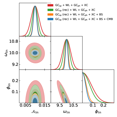
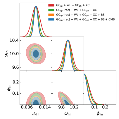
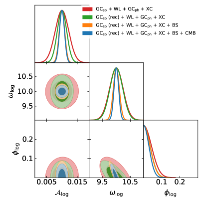
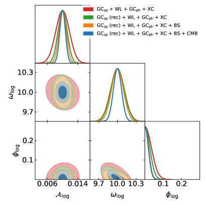
Figure 6: Fisher-forecast marginalised two-dimensional contours and one-dimensional probability distribution functions from Euclid on the primordial feature parameters for the LIN model with $\omega_{\rm lin}=10$ (top panels) and the LOG model with $\omega_{\rm log}=10$ (bottom panels). Left (right) panels correspond to the pessimistic (optimistic) setting for GC_sp+WL+GC_ph+XC (red), GC_sp+WL+GC_ph+XC with numerical reconstruction of GC_sp (green), GC_sp(rec)+WL+GC_ph+XC in combination with Euclid GC_sp bispectrum (orange), and their combination plus SO-like CMB (blue).

Appendix A

In Figs. 7 and 8, we compare the ratio between the matter power spectrum with primordial oscillations to the one obtained with a power-law PPS at redshift $z=0$. We show analytic results obtained with PT at LO (blue) and NLO (orange) versus linear theory predictions (grey) and the nonlinear results obtained from N-body simulations (green).

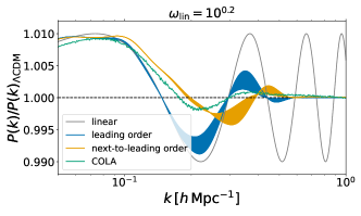
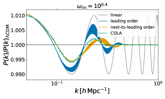
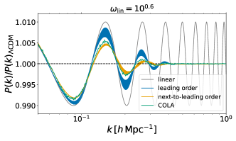
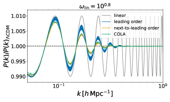
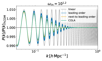
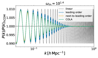
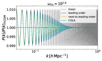
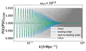
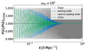
Figure 7: Ratio of IR resummed matter power spectrum at LO (blue) and NLO (orange) obtained for the linear oscillations to the one obtained with a power-law PPS at redshift $z=0$ varying the IR separation scale $k_{\rm S}=\epsilon k$ with $\epsilon\in(0.3,\,0.7)$. Also shown are the linear results (grey) and the ones obtained from N-body simulations (green).

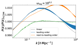
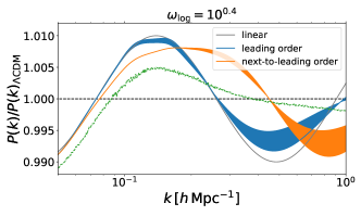
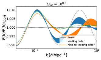
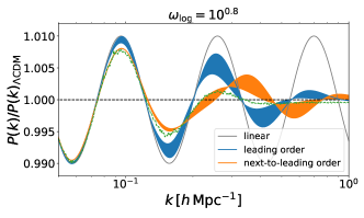
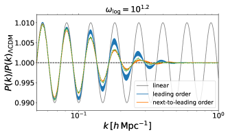
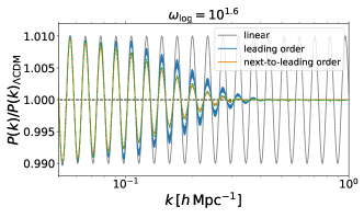
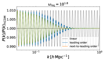
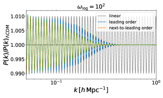
Figure 8: As in Fig. 7, but for the logarithmic oscillations.

Appendix B

In Fig. 9, we compare the wiggle $O_{\rm w}(k)$, which is the ratio between the wiggled and no-wiggle $P(k)$, for all 20 wiggled models: linear models in the first two rows and logarithmic models in the bottom two rows as shown by the legend. The four subpanels of each row, from bottom to top, are the results for $z=1.5$, $1.0$, $0.5$, and $0$. Linear theory predictions (which in practice are replaced by the measured $P(k)$ from the initial condition snapshots at $z=9$) are shown by black solid curves, while the measurements from the fully nonlinear and reconstructed matter density fields are shown by blue solid and orange dashed curves.

Structure formation greatly damps the wiggles, and this impact is strongest for the low-frequency wiggle models, given that there are fewer peaks in the $k$ range shown. The extreme example is $\omega_{\rm log}=10^{0.2}$, for which at $z<1$ the only peak in the entire $k$ range shown here is completely invisible. Reconstruction is expected to be useful here, as shown by the orange curves in the corresponding panels. Even for models with very high wiggle frequencies, e.g. $\omega_{\rm log}=10^{2}$, the wiggles can be well reconstructed down to $k\simeq 1\,h\,{\rm Mpc}^{-1}$.

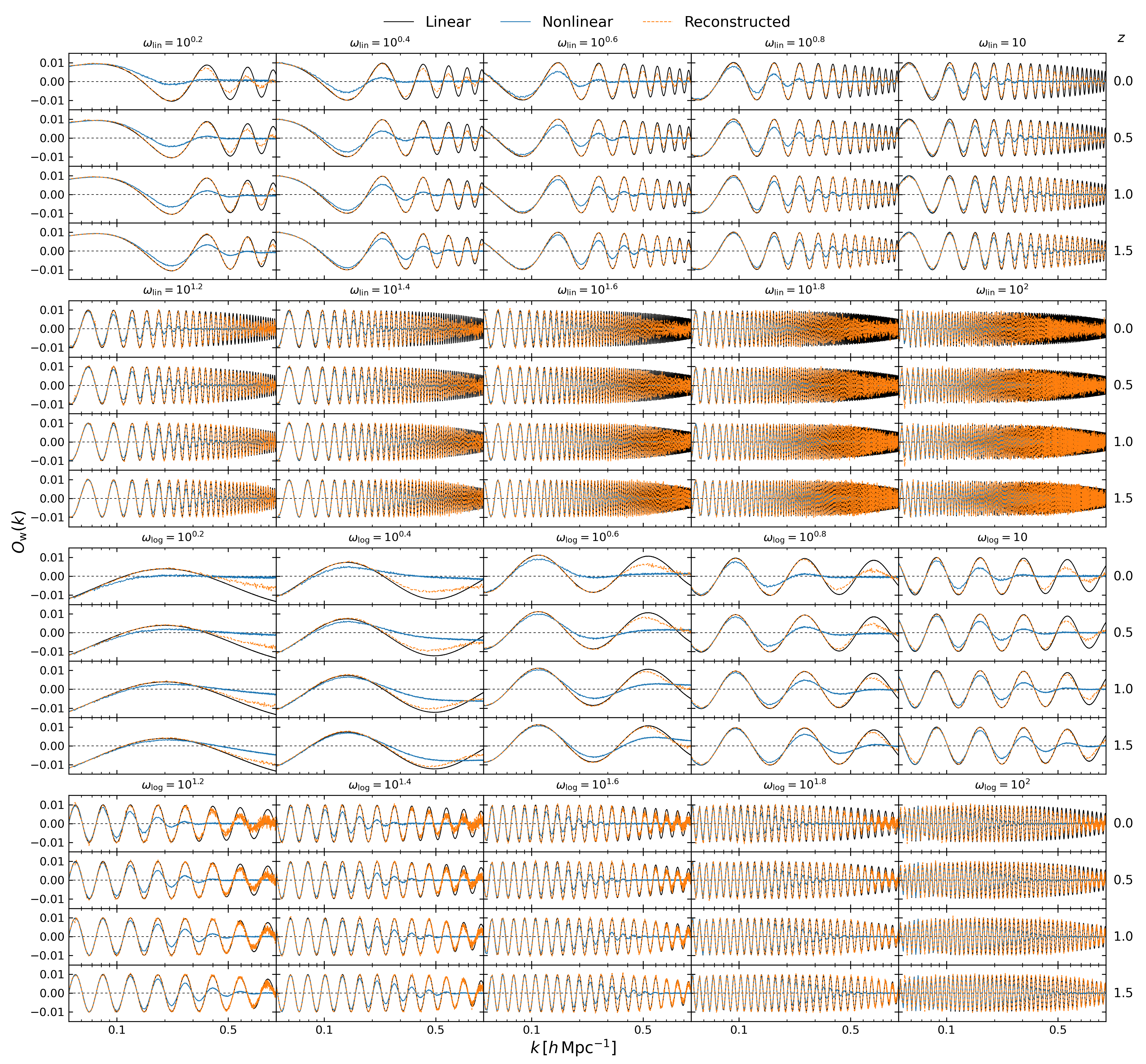
Figure 9: The wiggle spectra $O_{\rm w}(k)$ of the linear (black solid curves), nonlinear (blue solid curves) and reconstructed (orange dashed curves) density fields for the 20 selected feature models. Each of the rows is respectively for the redshifts marked on the right. The linear $O_{\rm w}(k)$ are measured from the initial conditions at $z=9$, the nonlinear $O_{\rm w}(k)$ are from the output snapshots of DM, and the reconstructed $O_{\rm w}(k)$ are from the reconstructed density fields.