Flux-pulse-assisted Readout of a Fluxonium Qubit

Abstract

Much attention has focused on the transmon architecture for large-scale superconducting quantum devices, however, the fluxonium qubit has emerged as a possible successor. With a shunting inductor in parallel to a Josephson junction, the fluxonium offers larger anharmonicity and stronger protection against dielectric loss, leading to higher coherence times as compared to conventional transmon qubits. The interplay between the inductive and Josephson energy potentials of the fluxonium qubit leads to a rich dispersive shift landscape when tuning the external flux. Here we propose to exploit the features in the dispersive shift to improve qubit readout. Specifically, we report on theoretical simulations showing improved readout times and error rates by performing the readout at a flux bias point with large dispersive shift. We expand the scheme to include different error channels, and show that flux-pulse-assisted readout offers 5 times improvement in signal to noise ratio after 200 ns integration time. Moreover, we show that the performance improvement persists in the presence of finite measurement efficiency combined with quasi-static flux noise. We suggest energy parameters for the fluxonium architecture that will allow for the implementation of our proposed flux-pulse-assisted readout scheme.

I Introduction

Two important prerequisites for meaningful quantum information processing are the ability to apply fast, accurate qubit gates and subsequently perform readout of the quantum state with high fidelity. High fidelity single shot measurement of superconducting qubits can be achieved through the exploitation of circuit quantum electrodynamics (cQED) [1, 2, 3]. By coupling a qubit to a far detuned resonator, where the qubit-resonator detuning is much larger than the coupling strength and resonator linewidth, we reach the dispersive limit. In this regime, we can perform a quantum non-demolition (QND) measurement through probing the readout resonator with coherent microwave pulses and measuring the transmitted and reflected signals that are correlated with the qubit state [4, 1, 3]. This method of measurement was initially implemented with a Cooper pair box and later in a transmon architecture, and can be further extended to other, novel superconducting device architectures such as the fluxonium [3, 1, 5]. The fluxonium qubit, initially introduced by Ref. [6], is composed of a Josephson junction shunted by a capacitive and an inductive element. The qubit can be biased via an external magnetic flux applied through the loop made up of the non-linear Josephson junction and the inductor. Ideally, fluxonium qubits have maximal coherence and relaxation times when operated with an externally applied flux bias of $\Phi_{ext}/\Phi_{0}=0.5$, also known as the “sweet-spot,” where $\Phi_{0}=h/(2e)$ is the magnetic flux quantum. At this point, the qubit is protected to first-order against flux noise and charge noise is exponentially suppressed [6, 7, 8, 9, 10].

As the interest in fluxonium qubits as a promising contender for quantum computation continues to grow due to their large anharmonicity and long coherence times, it is increasingly important to optimize all aspects of the fluxonium qubit such as minimizing readout time while increasing the fidelity [11, 9]. At the half flux quantum point, it is desirable to have a small dispersive shift to mitigate dephasing due to residual photons in the readout resonator [12]. However, this in turn makes fast readout challenging because longer integration times are required to differentiate the qubit states with high accuracy. To combat these opposing requirements, we propose the idea of using a rapid flux pulse to tune the qubit to a flux bias point where there is a large dispersive shift in order to perform the readout. Recent work with transmon qubits has demonstrated state-of-the-art measurement fidelity resulting, in part, from dynamic tuning of the qubit frequency in order to reduce the qubit-resonator detuning and thus, increase the dispersive interaction strength [13]. This effect had been experimentally shown previously with transmon architectures in Refs. [14, 15], and we now aim to expand the principle to fluxonium qubits. We also show this proposal to be robust, not only to variations in energy parameters due to fabrication imperfections, but also in the presence of limited measurement efficiency and quasi-static flux noise. Ideally, the readout scheme should not be more sensitive to flux noise than other operations, so to put the simulations of quasi-static flux noise in context, we simulate optimized single qubit gates in the presence of this noise, as well [11, 16, 17, 9].

In this work, we first present results of simulations performed to identify an appropriate energy parameter regime of the fluxonium qubit for implementation of fast readout via examination of the dispersive shift landscape. We proceed to examine how the signal to noise ratio and measurement fidelity are improved as a result of using a high dispersive shift during readout. Finally, using the same energy parameters, we investigate how imperfect measurement efficiency and the presence of quasi-static flux noise that generates a constant flux bias offset affects the achievable signal to noise ratio during readout and the fidelity of single qubit gates.

II Fluxonium Qubit

An effective lumped element circuit diagram of a fluxonium qubit coupled to a readout resonator is depicted in Fig. 1. The Hamiltonian used to describe the fluxonium qubit is

$$\hat{H}_{\mathrm{fluxonium}}=4E_{C}\hat{n}^{2}+\frac{1}{2}E_{L}\hat{\phi}^{2}-E_{J}\mathrm{cos}(\hat{\phi}-\phi_{ext}),$$ (1)

where $E_{C}$ is the charging energy of the fluxonium island, $E_{L}$ is the inductive energy of the inductor, $E_{J}$ is the Josephson energy, $\phi_{ext}=2\pi(\Phi_{ext}/\Phi_{0})$, and $\Phi_{ext}$ is the physical flux threading the loop shared by the Josephson junction and the inductor. It is convenient to simulate the fluxonium Hamiltonian in the harmonic oscillator basis where the charge operator is defined as $\hat{n}=\frac{-i}{\sqrt{2}\phi_{0}}(\hat{c}-\hat{c}^{\dagger}$) and the flux operator takes the form $\hat{\phi}=\frac{\phi_{0}}{\sqrt{2}}(\hat{c}+\hat{c}^{\dagger})$, where $\phi_{0}=(8E_{C}/E_{L})^{1/4}$, and $\hat{c}$ and $\hat{c}^{\dagger}$ are the annihilation and creation operators, respectively, of the qubit basis states [18].

Figure 1: Effective circuit model of a fluxonium qubit capacitively coupled to a resonator, where $E_{J}$, $E_{C}$, and $E_{L}$ are the Josephson, capacitive, and inductive energies, respectively, $\Phi_{ext}$ is the flux threading the depicted loop, $g$ is the coupling strength between the qubit and readout resonator, and $\omega_{r}$ is the frequency of the readout resonator.

The resonator and coupling between the resonator and qubit, where the coupling term assumes the rotating wave approximation, are modeled by

$$\hat{H}_{\mathrm{{resonator}}}=\hbar\omega_{r}(\hat{a}^{\dagger}\hat{a}+\frac{1}{2}),$$ (2)

$$\hat{H}_{\mathrm{{coupling}}}=\hbar g(\hat{a}\hat{c}^{\dagger}+\hat{a}^{\dagger}\hat{c}).$$ (3)

In these equations, $\omega_{r}=1/\sqrt{LC}$ is the resonant frequency of the resonator, $g$ is the coupling strength mediated by the coupling capacitor, and $\hat{a}^{\dagger}$ and $\hat{a}$ are the creation and annihilation operators of the resonator.

III Dispersive Shift Landscape

We can simplify the total Hamiltonian by assuming the fluxonium qubit acts as a two level system, and thus use the Jaynes-Cummings model under the rotating wave approximation to describe the system in Fig. 1. Operating in the dispersive regime where the detuning between the qubit and resonator is much larger than the coupling strength ($\left|\Delta\right|=\left|\omega_{r}-\omega_{q}\right|\gg g$), the Hamiltonian can be expanded to second order in $g/\Delta$ using perturbation theory [19]

$$\hat{H}_{\mathrm{{JC}}}=\hbar\left(\omega_{r}+\frac{g^{2}}{\Delta}\hat{\sigma}_{z}\right)\hat{a}^{\dagger}\hat{a}+\frac{\hbar}{2}\left(\omega_{q}+\frac{g^{2}}{\Delta}\right)\hat{\sigma}_{z}.$$ (4)

In this equation, $\omega_{q}$ represents the qubit frequency and $\hat{\sigma}_{z}$ is the Pauli-Z operator.

From the first term in Eq. (4), it becomes evident that the resonator frequency is dependent on the state of the qubit. The dispersive shift refers to the amount by which the qubit state dresses the bare resonator frequency and is denoted by $\chi=g^{2}/\Delta$. However, this approximate Hamiltonian neglects levels outside of the computational subspace which play an important role in the qubit-resonator interaction for fluxonium qubits [18]. Therefore, we instead numerically diagonalize the Hamiltonian for the qubit-resonator coupled system and calculate the dispersive shift, where we use the basis notation $\left|\mathrm{qubit,resonator}\right\rangle$, which identifies the dressed state closest to the corresponding bare state

$$2\chi=(\omega_{\left|1,1\right\rangle}-\omega_{\left|1,0\right\rangle})-(\omega_{\left|0,1\right\rangle}-\omega_{\left|0,0\right\rangle}).$$ (5)

We aim to satisfy a moderately small dispersive shift on the order of $\chi/2\pi=0.5-1$ MHz at $\Phi_{ext}/\Phi_{0}=0.5$, as this gives a slow dephasing rate between approximately 3-10 kHz ($T_{2}\approx$ 100-330 $\mu$s in the limit as $T_{1}\rightarrow\infty$) with a conservative choice of effective resonator temperature of 80 mK and a resonator linewidth of $\kappa=5$ MHz [12]. At an optimal readout point, we desire a large dispersive shift on the order of $\chi/2\pi=5-10$ MHz. Sub 100 ns readout has been demonstrated with dispersive shift values in this range for transmon qubits [20]. Another criterion to satisfy is having minimal avoided crossings in the dispersive shift between $\Phi_{ext}/\Phi_{0}=0.5$ and the chosen readout point. This requirement is to avoid coherently swapping excitations between the resonator and qubit while flux tuning to the readout point.

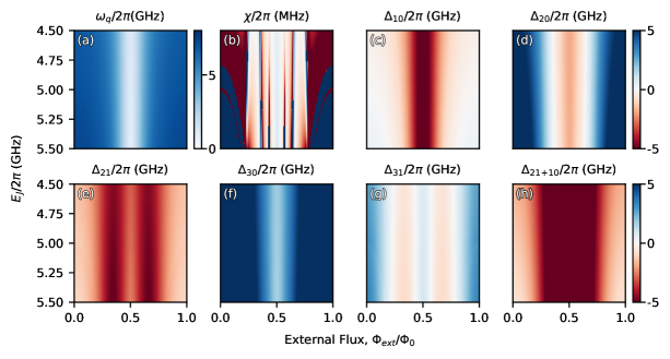
Figure 2: (a) Qubit transition frequency, (b) dispersive shift, and (c-h) detuning of various fluxonium transitions (denoted by the subscripts of $\Delta$) from the bare resonator frequency as a function of $E_{J}/2\pi$ (4.5-5.5 GHz) and external flux, where $E_{C}/2\pi=1.25$ GHz, $E_{L}/2\pi=1.5$ GHz, $\omega_{r}/2\pi=7$ GHz, and $g/2\pi=50$ MHz. The maximum and minumum of (b) are $\pm$5 MHz and for (c-h) they are $\pm$5 GHz to provide visual clarity. Values outside of this range take on the color corresponding to the maximum or minimum value, depending on the sign. Panels (b-h) share the same color bar, which is depicted to the right of panels d and h.

In Fig. 2(a) and (b), we numerically solve for the fluxonium qubit transition, $\omega_{q}$, and for the dispersive shift, $\chi$, respectively, and while the behavior of $\omega_{q}$ is rather smooth, we notice many rapidly changing features in $\chi$. Since the fluxonium qubit is not restricted by stringent selection rules away from flux biases equalling half-integer and integer flux quanta, higher order transitions can interact with the readout resonator giving rise to a large dispersive shift, see Fig. 2(c-h) where we display the detuning between various dressed higher order transitions and the bare readout resonator frequency. Ref. [18] elucidated the fact that each higher order transition contributes to the effective dispersive shift. The dispersive shift caused by a given transition $i\rightarrow j$ is proportional to $\left|\left\langle i\right|\hat{n}\left|j\right\rangle\right|^{2}/\Delta_{ij}$. Thus, as $\Delta_{ij}\rightarrow 0$, we expect an increase in the magnitude of the dispersive shift. At small detunings, the interaction is no longer considered dispersive and, thus, we want to avoid these regions as the dynamics will be dominated by a coherent swap interaction between the fluxonium and the resonator. By matching the regions of $\Delta_{ij}=0$ in Fig. 2(c-h) with regions of diverging dispersive shift, $\chi$, in Fig. 2(b), we identify which specific transition causes each divergence in the dispersive shift. For instance, the two dark, narrow lines in Fig. 2(b) closest to the half flux quantum point are caused by the $\left|3\right\rangle\leftrightarrow\left|1\right\rangle$ transition being on resonance with the readout resonator.

IV Readout

Fluxonium qubits with frequencies around 1 GHz or lower at the sweet-spot have shown consistently high $T_{1}$ times exceeding 100 $\mu$s [21]. To satisfy this requirement on the qubit frequency, as well as the requirements for the dispersive shift discussed in the previous section, we pick appropriate energy parameters for the fluxonium based on the results in Fig. 2. We propose to use a fluxonium qubit with the parameters $E_{J}/2\pi=4.75$ GHz, $E_{C}/2\pi=1.25$ GHz, and $E_{L}/2\pi=1.5$ GHz for implementing a flux pulse during readout to improve fidelity and speed. These values were chosen to keep both the qubit frequency and dispersive shift low at the sweet-spot, as altering one of the energy parameters results in a decrease in one value, but increase in the other. Additionally, targeting these values ensures that in the case of deviations due to fabrication imperfections, the proposed readout scheme can still be implemented. We note that the fluxonium qubit is symmetric about the sweet-spot, so we focus our discussion on values of $\Phi_{ext}/\Phi_{0}\geq 0.5$ for the rest of this section.

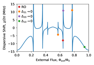
Figure 3: Dispersive shift as a function of external flux where $E_{J}/2\pi=4.75$ GHz, $E_{C}/2\pi=1.25$ GHz, and $E_{L}/2\pi=1.5$ GHz. The targeted readout (RO) point is marked with a red circle and the other markers denote where a certain qubit transition, $i\rightarrow j$, and the resonator are near or on resonance, denoted by $\Delta_{ij}\rightarrow 0$.

In order to simulate our system with the specified parameters, we use a readout resonator frequency of $\omega_{r}/2\pi=7$ GHz and a coupling strength of $g/2\pi=50$ MHz. At the half flux quantum point, $\chi/2\pi\approx 0.53$ MHz and $\omega_{q}/2\pi\approx 1.05$ GHz. The proposed readout point is denoted with a red circle in Fig. 3, which sits at a flux bias of $\Phi_{ext}/\Phi_{0}\approx 0.64$, where $\chi/2\pi\approx-8$ MHz, $\omega_{q}/2\pi\approx 4.6$ GHz, and $\Delta_{10}/2\pi=-2.4$ GHz. The large dispersive shift arises due to $\Delta_{20}$ approaching zero. At the specific value we propose, we have $\Delta_{20}/2\pi=-67$ MHz which places the system at the edge of the dispersive limit with $g_{20}^{2}/\Delta_{20}=2\pi\times-5$ MHz. Here, $g_{20}/2\pi$ = $(g/2\pi)\left|\left\langle 2\right|\hat{n}\left|0\right\rangle\right|$ = 18.32 MHz. From Fig. 3, it is evident that we must traverse a point at which the $\left|3\right\rangle\leftrightarrow\left|1\right\rangle$ qubit transition is resonant with the resonator around $\Phi_{ext}/\Phi_{0}\approx 0.575$. We numerically calculate $g_{31}/2\pi=5.81$ MHz from the size of the anticrossing, which yields a swap time of roughly 43 ns. From the Jaynes-Cummings model, the swap time is defined as $\pi/2g_{ij}$, and is the time it takes for an excitation to be exchanged between the qubit subspace and resonator given that they are on resonance. The swap time sets an upper limit on the ramp time of the flux pulse.

In order to achieve high measurement fidelity, we aim to perform a strong measurement in a short amount of time in order to avoid relaxation of the qubit of interest. We can quantify the strength of the measurement using the signal to noise ratio (SNR) as a quantitative metric. This value is the ratio between the separation of the mean of the $\left|0\right\rangle$ and $\left|1\right\rangle$ state projections in the (I,Q) plane, and the total standard deviation of the two signal distributions which typically take on a Gaussian profile [22, 23]. The separation between the distributions grows linearly in time, $t$, compared to the width of the distributions which scales as $\sqrt{t}$ [22]. We are in the strong measurement regime when the SNR is greater than unity and the two states can be distinguished because the distributions have separated after a certain amount of integration time.

We can use the Langevin equation in the context of input-output formalism in order to numerically simulate the output field of a resonator when probed with a coherent input field via a capacitively coupled drive line. This is expressed as

$$\dot{\hat{a}}=-i\chi\hat{\sigma}_{z}\hat{a}-\frac{1}{2}\kappa\hat{a}-\sqrt{\kappa}\hat{a}_{in},$$ (6)

$$\hat{a}_{out}=\hat{a}_{in}+\sqrt{\kappa}\hat{a},$$ (7)

where Eq. (7) is the boundary condition for Eq. (6), $\hat{a}_{in}$ is the coherent input field such that $\langle\hat{a}_{in}\rangle$=$-\epsilon/\sqrt{\kappa}$, $\hat{a}$ is the intracavity field, $\hat{a}_{out}$ is the output field, and $\kappa$ is the photon decay rate into the drive line or the linewidth of the resonator [24, 25, 26]. Assuming the resonator is in a coherent state as we probe it with a classical signal, Eq. (6) can alternatively be solved in terms of the coherent state amplitude, $\alpha$, from

$$\dot{\alpha}=-i\chi\left\langle\hat{\sigma}_{z}\right\rangle\alpha-\frac{1}{2}\kappa\alpha-\sqrt{\kappa}\alpha_{in},$$ (8)

where $\alpha_{(in/out)}$ = $\left\langle\hat{a}_{(in/out)}\right\rangle$. Eq. (8) has the solutions

$$\begin{split}&\alpha_{\pm}=\frac{\epsilon}{\sqrt{\kappa}}e^{-i\phi_{qb}\left\langle\hat{\sigma}_{z}\right\rangle}\\ &\times\left[1-2\mathrm{cos}\left(\frac{\phi_{qb}}{2}\right)e^{\left(-i\chi\tau\left\langle\hat{\sigma}_{z}\right\rangle-\frac{\kappa\tau}{2}+i\frac{\phi_{qb}}{2}\left\langle\hat{\sigma}_{z}\right\rangle\right)}\right].\end{split}$$ (9)

From Eq. (9), $\alpha_{+}$ ($\alpha_{-}$) is obtained when $\left\langle\hat{\sigma}_{z}\right\rangle$ = +1 (-1), corresponding to the qubit eigenstate $\left|0\right\rangle$ ($\left|1\right\rangle$). Additionally, $\tau$ is the integration time, $\epsilon$ is the driving amplitude of the input field, and $\phi_{qb}$ is the phase shift of the output field caused by the qubit, defined as

$$\phi_{qb}=2\mathrm{arctan}\left(\frac{2\chi}{\kappa}\right).$$ (10)

We can choose $\epsilon$ based on the targeted mean photon number by solving for $\overline{n}$ in the steady state in terms of the drive amplitude

$$\epsilon=\sqrt{\overline{n}\left(\frac{\kappa^{2}}{4}+\chi^{2}\right)}.$$ (11)

Once we have found $\alpha_{\pm}$, we can find $\alpha_{out}$ via the equation

$$\alpha_{out}=\alpha_{in}+\sqrt{\kappa}\alpha.$$ (12)

We can describe the signal to noise ratio in terms of the measurement operator $\hat{M}$

$$\hat{M}(\tau)=\sqrt{\kappa\eta}\int_{0}^{\tau}[\hat{a}_{out}^{\dagger}(t)+\hat{a}_{out}(t)]dt,$$ (13)

where $\eta$ is the measurement efficiency. We denote $\left\langle\hat{M}\right\rangle$ as $M_{S}$ and the noise operator as $\hat{M}_{N}$ = $\hat{M}$-$\left\langle\hat{M}\right\rangle$, following the convention in Ref. [26]. The equation describing the signal to noise ratio then reads as

$$SNR=\frac{|M_{S,\eta,\left|0\right\rangle}-M_{S,\eta,\left|1\right\rangle}|}{\left[\left\langle\hat{M}_{N,\left|0\right\rangle}^{2}\right\rangle+\left\langle\hat{M}_{N,\left|1\right\rangle}^{2}\right\rangle\right]^{1/2}}.$$ (14)

We can evaluate $\left\langle\hat{M}_{N}^{2}\right\rangle$ to $\kappa\tau$ since we are using a coherent input field.

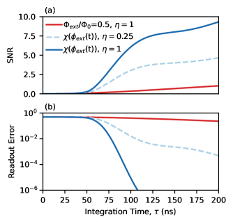
Figure 4: Comparison of readout at the half flux quantum point where $\Phi_{ext}/\Phi_{0}=0.5$ and $\chi/2\pi=0.527$ MHz (red) versus readout incorporating a flux pulse with 50 ns rise time to $\Phi_{ext}/\Phi_{0}=0.641$ with $\chi/2\pi=-7.95$ MHz for measurement efficiencies of 25$\%$ (light blue, dashed) and 100$\%$ (dark blue, solid). (a) Signal to noise ratio and (b) readout error as a function of integration time.

Combining these formulas, we first calculate the SNR for conventional fluxonium readout where $\Phi_{ext}/\Phi_{0}=0.5$ and remains static, see red lines in Fig. 4. At the half flux quantum point, the dispersive shift is $\chi/2\pi=0.527$ MHz and with a resonator linewidth of $\kappa/2\pi=5$ MHz, perfect measurement efficiency, and $\bar{n}=10$, we obtain an SNR of 1 after about 200 ns. Following our proposal, we next discern the effect of performing readout during flux tuning of the qubit. We numerically solve the Langevin equation using an explicit time dependent dispersive shift $\chi(\phi_{ext},t)=\chi(\phi_{ext}(t))$, following the behavior shown in Fig. 3 and assuming the flux increases linearly from $\Phi_{ext}/\Phi_{0}=0.5$ to the target flux of $\Phi_{ext}/\Phi_{0}=0.641$ during the first 50 ns of the readout. The SNR slowly increases during the ramp time of the flux pulse and then increases more rapidly once the steady value of $\Phi_{ext}/\Phi_{0}=0.641$ is reached, see blue lines in Fig. 4. Assuming 100$\%$ measurement efficiency, the SNR is around 10 after 200 ns, giving an order of magnitude improvement in the SNR as compared to static readout at the sweet-spot. With a realistic experimental measurement efficiency of 25$\%$, after 200 ns the SNR is still about 5 times larger than the SNR obtained with perfect measurement efficiency when readout is performed at the sweet-spot. Thus, we can more rapidly distinguish the two qubit states with high certainty via the exploitation of a strong dispersive shift. We use a long flux pulse rise time in these simulations to numerically demonstrate proof of principle and show that we still see a substantial improvement in measurement time, and potential additional speedup could be achieved with pulse shaping [27].

From the signal to noise ratio, we can also extract the measurement error from

$$\mathrm{error}=\frac{1}{2}\mathrm{erfc}\left(\frac{\mathrm{SNR}}{2}\right),$$ (15)

with

$$\mathrm{erfc}(x)=1-\frac{2}{\sqrt{\pi}}\int_{0}^{x}e^{-t^{2}}dt,$$

which is displayed in Fig. 4(b).

As expected, the readout error trends towards zero for large times, although much more rapidly for the case where we flux tune to the suggested readout point. Using the proposed flux pulsing scheme, an error of $10^{-3}$ is reached in roughly 180 ns for the case of 25$\%$ measurement efficiency, compared to 940 ns if readout is performed at the half flux quantum point with perfect measurement efficiency. It is important to note that in practice we will not only be limited by finite measurement efficiency, but also the relaxation time of the qubit and potential measurement-induced state transitions, which were not accounted for in these simulations [14, 28].

V Quasi-static Flux Noise

Although the fluxonium qubit benefits from long coherence times partially afforded by the first-order insensitivity to flux noise at the sweet-spot, our proposed protocol requires flux-pulsing to a bias point that has an increased susceptibility to flux noise. Additionally, Ref. [29] showed that the dominant noise mechanism in fluxonium qubits transitions from dielectric loss to 1/$f$ noise for frequencies at and below about $\omega\approx 2k_{B}T_{\mathrm{eff}}/\hbar$, with quasi-static 1/$f$ noise, varying from one pulse sequence to the next, resulting in dephasing [30]. While additional dephasing during readout is irrelevant as a strong measurement inherently dephases the qubit, we need to verify that the flux-pulse-assisted measurement performance is not limited by potential flux noise.

In this section, we simulate the presence of quasi-static flux noise by adding a constant flux bias offset of $\delta$ during flux-pulse-assisted readout, assuming 25$\%$ measurement efficiency. We average over 50 iterations of $\delta$ for 3 different scaling factors. In this context, $\delta=\varepsilon x\Phi_{0}$, where $\varepsilon$ is a scaling factor of $10^{-2},10^{-3},\mathrm{or}$ $10^{-4}$, and $x$ is a random number sampled from a Gaussian distribution with a mean of $\mu=0$ and a variance of $\sigma^{2}=1$, for each iteration. The literature commonly reports flux noise amplitudes on the order of 1-10 $\mu\Phi_{0}$ observed in superconducting qubit devices [31, 32, 33, 34]. Thus, the amount of noise we add to our numerical simulations reflects flux noise significantly larger than that observed in state-of-the-art experiments. As displayed in Fig. 5(a), for the extreme case of $\varepsilon=10^{-2}$, our SNR after 200 ns is 3 times larger than the SNR with a static readout at sweet-spot with perfect measurement efficiency (refer to red line of Fig. 4(a)). This corresponds to a readout error of roughly 4$\%$. In the cases of $\varepsilon=10^{-3}$ or $10^{-4}$, there is no substantial deviation from the readout achievable in the presence of zero quasi-static flux noise.

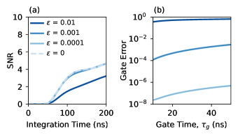
Figure 5: Comparison of (a) readout signal to noise ratio obtained using flux-pulse-assisted readout with a measurement efficiency of 25$\%$ and (b) single qubit gate fidelity of a Pauli-X gate with varying amounts of quasi-static flux noise added in the form of a constant offset, $\delta$, where $\delta$ = $\varepsilon a\Phi_{0}$ and $a$ is a value sampled randomly from a normal Gaussian distribution.

For comparison, we also simulate the single qubit gate fidelity of a Pauli-X gate with a DRAG pulse performed at the sweet-spot in the presence of varying degrees of quasi-static flux noise in order to further characterize the achievable quality of qubit operations in the presence of this decoherence channel. We add the flux noise offset in the same manner which was done for the readout simulations previously discussed. Prior to adding the noise, we first optimize the performance of the $X_{\pi}$ rotation.

In order to model these single qubit gates, we add a drive term to the Hamiltonian of the fluxonium-resonator coupled system [Eq. (1-3)]. We assume the qubit is capacitively coupled to a microwave drive line that receives signals from room temperature electronics, of which experimental parameters including pulse shape, amplitude, duration, frequency, and phase can be altered.

The envelope function used to describe the shape of the in-phase pulse component is

$$s(t)=\frac{1}{2}\left(1-\mathrm{cos}\left(\frac{2\pi(t)}{\tau_{g}}\right)\right).$$ (16)

We opt for a sinusoidal envelope function as in Ref. [9] in order to avoid the truncation that is necessary with a traditional Gaussian envelope function and to reduce the bandwidth of the pulse. A derivative removal by adiabatic gate (DRAG) pulse is also applied in the out-of-phase component to help correct for leakage and pulse errors, as has been done before in transmon qubits and has been theoretically explored in scalable fluxonium architectures [23, 35, 9]. The envelope function of this pulse takes the form

$$s^{\prime}(t)=\frac{\lambda}{\alpha}\frac{\partial s(t)}{\partial t},$$ (17)

where $\lambda$ is a scaling parameter and $\alpha$ is the qubit’s anharmonicity.

With this pulse shape defined, we can write the drive term of the Hamiltonian as

$$\hat{H}_{\mathrm{drive}}=\varepsilon_{d}\hat{n}[2s(t)\mathrm{sin}(\omega_{d}(t))+s^{\prime}(t)\mathrm{cos}(\omega_{d}(t))],$$ (18)

where $\varepsilon_{d}$ is the drive amplitude and $\omega_{d}$ is the frequency of the drive signal.

We first optimize over $\varepsilon_{d}$ and $\lambda$, assuming that $\omega_{d}=\omega_{q,\varphi_{ext}=\pi}$, for gate times ranging from 10-50 ns. We subsequently add the flux noise offset to the single qubit gate performance with optimized parameters. These results are presented in Fig. 5(b). In the noisiest case simulated with $\varepsilon=10^{-2}$, our single qubit gate error has a high value of 36$\%$ with a gate time of 10 ns, which is an order of magnitude worse than the readout error induced by this level of flux noise. If we compare the single qubit gate error curves in the cases of $\varepsilon=10^{-3}$ and $10^{-4}$, we see that one order of magnitude increase in quasi-static flux noise degrades the gate error by 4 orders of magnitude. Thus, we observe that our flux-pulse-assisted readout scheme is more robust than optimized single qubit gates in the face of quasi-static 1/$f$ flux noise.

VI Conclusion and Outlook

In summary, we present a proposal for performing flux-pulse-assisted, fast, high fidelity readout of a fluxonium qubit with optimized energy parameters. We suggest appropriate values of Josephson, capacitive, and inductive energy for a fluxonium qubit which will enable our readout proposal based on the simulated dispersive shift landscape. Then, we proceed to show the improvement in measurement speed that can be obtained by exploiting a large dispersive shift when the qubit is detuned from the sweet-spot. In this work, we do not explicitly consider swap dynamics or changes in the dispersive shift due to AC Stark shifting during measurement, however, we expect this can be compensated for through flux pulse calibration. Pulse shaping techniques may also be utilized to further reduce the time required for the scheme. Finally, we present the readout SNR and single qubit gate fidelity achievable in the presence of quasi-static flux noise. Our simulated results show robust improvement in both readout speed and fidelity when the proposed protocol is implemented.

Data Availability

The code used to generate these numerical results is available at https://github.com/AndersenQubitLab/FluxPulseAssistedFluxonium.

References

- Blais et al. [2004] A. Blais, R.-S. Huang, A. Wallraff, S. M. Girvin, and R. J. Schoelkopf, Cavity quantum electrodynamics for superconducting electrical circuits: An architecture for quantum computation, Physical Review A 69, 062320 (2004).
- Schoelkopf and Girvin [2008] R. Schoelkopf and S. Girvin, Wiring up quantum systems, Nature 451, 664 (2008).
- Wallraff et al. [2004] A. Wallraff, D. I. Schuster, A. Blais, L. Frunzio, R.-S. Huang, J. Majer, S. Kumar, S. M. Girvin, and R. J. Schoelkopf, Strong coupling of a single photon to a superconducting qubit using circuit quantum electrodynamics, Nature 431, 162 (2004).
- Braginsky et al. [1980] V. B. Braginsky, Y. I. Vorontsov, and K. S. Thorne, Quantum nondemolition measurements, Science 209, 547 (1980).
- Koch et al. [2007] J. Koch, M. Y. Terri, J. Gambetta, A. A. Houck, D. I. Schuster, J. Majer, A. Blais, M. H. Devoret, S. M. Girvin, and R. J. Schoelkopf, Charge-insensitive qubit design derived from the cooper pair box, Physical Review A 76, 042319 (2007).
- Manucharyan et al. [2009] V. E. Manucharyan, J. Koch, L. I. Glazman, and M. H. Devoret, Fluxonium: Single cooper-pair circuit free of charge offsets, Science 326, 113 (2009).
- Gyenis et al. [2021] A. Gyenis, A. Di Paolo, J. Koch, A. Blais, A. A. Houck, and D. I. Schuster, Moving beyond the transmon: Noise-protected superconducting quantum circuits, PRX Quantum 2, 030101 (2021).
- Lin et al. [2018] Y.-H. Lin, L. B. Nguyen, N. Grabon, J. San Miguel, N. Pankratova, and V. E. Manucharyan, Demonstration of protection of a superconducting qubit from energy decay, Physical review letters 120, 150503 (2018).
- Nguyen et al. [2022] L. B. Nguyen, G. Koolstra, Y. Kim, A. Morvan, T. Chistolini, S. Singh, K. N. Nesterov, C. Jünger, L. Chen, Z. Pedramrazi, et al., Scalable high-performance fluxonium quantum processor, arXiv preprint arXiv:2201.09374 (2022).
- Koch et al. [2009] J. Koch, V. Manucharyan, M. Devoret, and L. Glazman, Charging effects in the inductively shunted josephson junction, Physical review letters 103, 217004 (2009).
- Bao et al. [2022] F. Bao, H. Deng, D. Ding, R. Gao, X. Gao, C. Huang, X. Jiang, H.-S. Ku, Z. Li, X. Ma, et al., Fluxonium: an alternative qubit platform for high-fidelity operations, Physical Review Letters 129, 010502 (2022).
- Wang et al. [2019] Z. Wang, S. Shankar, Z. Minev, P. Campagne-Ibarcq, A. Narla, and M. H. Devoret, Cavity attenuators for superconducting qubits, Physical Review Applied 11, 014031 (2019).
- Swiadek et al. [2023] F. Swiadek, R. Shillito, P. Magnard, A. Remm, C. Hellings, N. Lacroix, Q. Ficheux, D. C. Zanuz, G. J. Norris, A. Blais, et al., Enhancing dispersive readout of superconducting qubits through dynamic control of the dispersive shift: Experiment and theory, arXiv preprint arXiv:2307.07765 (2023).
- Sank et al. [2016] D. Sank, Z. Chen, M. Khezri, J. Kelly, R. Barends, B. Campbell, Y. Chen, B. Chiaro, A. Dunsworth, A. Fowler, et al., Measurement-induced state transitions in a superconducting qubit: Beyond the rotating wave approximation, Physical review letters 117, 190503 (2016).
- Krinner et al. [2022] S. Krinner, N. Lacroix, A. Remm, A. Di Paolo, E. Genois, C. Leroux, C. Hellings, S. Lazar, F. Swiadek, J. Herrmann, et al., Realizing repeated quantum error correction in a distance-three surface code, Nature 605, 669 (2022).
- Moskalenko et al. [2022] I. N. Moskalenko, I. A. Simakov, N. N. Abramov, A. A. Grigorev, D. O. Moskalev, A. A. Pishchimova, N. S. Smirnov, E. V. Zikiy, I. A. Rodionov, and I. S. Besedin, High fidelity two-qubit gates on fluxoniums using a tunable coupler, npj Quantum Information 8, 1 (2022).
- Somoroff et al. [2021] A. Somoroff, Q. Ficheux, R. A. Mencia, H. Xiong, R. V. Kuzmin, and V. E. Manucharyan, Millisecond coherence in a superconducting qubit, arXiv preprint arXiv:2103.08578 (2021).
- Zhu et al. [2013] G. Zhu, D. G. Ferguson, V. E. Manucharyan, and J. Koch, Circuit qed with fluxonium qubits: Theory of the dispersive regime, Physical Review B 87, 024510 (2013).
- Schuster [2007] D. I. Schuster, Circuit Quantum Electrodynamics, Ph.D. thesis (2007).
- Walter et al. [2017] T. Walter, P. Kurpiers, S. Gasparinetti, P. Magnard, A. Potočnik, Y. Salathé, M. Pechal, M. Mondal, M. Oppliger, C. Eichler, et al., Rapid high-fidelity single-shot dispersive readout of superconducting qubits, Physical Review Applied 7, 054020 (2017).
- Nguyen et al. [2019] L. B. Nguyen, Y.-H. Lin, A. Somoroff, R. Mencia, N. Grabon, and V. E. Manucharyan, High-coherence fluxonium qubit, Physical Review X 9, 041041 (2019).
- Clerk et al. [2010] A. A. Clerk, M. H. Devoret, S. M. Girvin, F. Marquardt, and R. J. Schoelkopf, Introduction to quantum noise, measurement, and amplification, Reviews of Modern Physics 82, 1155 (2010).
- Krantz et al. [2019] P. Krantz, M. Kjaergaard, F. Yan, T. P. Orlando, S. Gustavsson, and W. D. Oliver, A quantum engineer’s guide to superconducting qubits, Applied Physics Reviews 6, 021318 (2019).
- Gardiner and Zoller [2004] C. Gardiner and P. Zoller, Quantum noise: a handbook of Markovian and non-Markovian quantum stochastic methods with applications to quantum optics (Springer Science & Business Media, 2004).
- Didier et al. [2015a] N. Didier, J. Bourassa, and A. Blais, Fast quantum nondemolition readout by parametric modulation of longitudinal qubit-oscillator interaction, Physical review letters 115, 203601 (2015a).
- Didier et al. [2015b] N. Didier, A. Kamal, W. D. Oliver, A. Blais, and A. A. Clerk, Heisenberg-limited qubit read-out with two-mode squeezed light, Physical review letters 115, 093604 (2015b).
- Bryon et al. [2022] J. Bryon, D. Weiss, X. You, S. Sussman, X. Croot, Z. Huang, J. Koch, and A. Houck, Experimental verification of the treatment of time-dependent flux in circuit quantization, arXiv preprint arXiv:2208.03738 (2022).
- Khezri et al. [2022] M. Khezri, A. Opremcak, Z. Chen, A. Bengtsson, T. White, O. Naaman, R. Acharya, K. Anderson, M. Ansmann, F. Arute, et al., Measurement-induced state transitions in a superconducting qubit: Within the rotating wave approximation, arXiv preprint arXiv:2212.05097 (2022).
- Sun et al. [2023] H. Sun, F. Wu, H.-S. Ku, X. Ma, J. Qin, Z. Song, T. Wang, G. Zhang, J. Zhou, Y. Shi, et al., Characterization of loss mechanisms in a fluxonium qubit, arXiv preprint arXiv:2302.08110 (2023).
- Bylander et al. [2011] J. Bylander, S. Gustavsson, F. Yan, F. Yoshihara, K. Harrabi, G. Fitch, D. G. Cory, Y. Nakamura, J.-S. Tsai, and W. D. Oliver, Dynamical decoupling and noise spectroscopy with a superconducting flux qubit, arXiv preprint arXiv:1101.4707 (2011).
- Braumüller et al. [2020] J. Braumüller, L. Ding, A. P. Vepsäläinen, Y. Sung, M. Kjaergaard, T. Menke, R. Winik, D. Kim, B. M. Niedzielski, A. Melville, et al., Characterizing and optimizing qubit coherence based on squid geometry, Physical Review Applied 13, 054079 (2020).
- Kou et al. [2017] A. Kou, W. Smith, U. Vool, R. Brierley, H. Meier, L. Frunzio, S. Girvin, L. Glazman, and M. Devoret, Fluxonium-based artificial molecule with a tunable magnetic moment, Physical Review X 7, 031037 (2017).
- Gustavsson et al. [2011] S. Gustavsson, J. Bylander, F. Yan, W. D. Oliver, F. Yoshihara, and Y. Nakamura, Noise correlations in a flux qubit with tunable tunnel coupling, Physical Review B 84, 014525 (2011).
- Yoshihara et al. [2006] F. Yoshihara, K. Harrabi, A. Niskanen, Y. Nakamura, and J. S. Tsai, Decoherence of flux qubits due to 1/f flux noise, Physical review letters 97, 167001 (2006).
- Gambetta et al. [2011] J. M. Gambetta, F. Motzoi, S. Merkel, and F. K. Wilhelm, Analytic control methods for high-fidelity unitary operations in a weakly nonlinear oscillator, Physical Review A 83, 012308 (2011).