Robin Hood model versus Sheriff of Nottingham model: transfers in population dynamics

Abstract

We study the problem of transfers in a population structured by a continuous variable corresponding to the quantity being transferred. The model is of Boltzmann type with kernels corresponding to the specific rules of the transfer process. We focus our interest on the well-posedness of the Cauchy problem in the space of measures and $L^{1}$. We characterize transfer kernels that give a continuous semiflow in the space of measures and $L^{1}$. We construct some examples of kernels that may be particularly interesting in economic applications. Our model considers blind money transfers between individuals. The two models are the “Robin Hood model”, where the richest individual unconditionally gives a fraction of their wealth to the poorest when a transfer occurs, and the other extreme, the “Sheriff of Nottingham model”, where the richest unconditionally takes a fraction of the poorest’s wealth. Between these two extreme cases is a continuum of intermediate models obtained by interpolating the kernels. We illustrate those models with numerical simulations and show that any small fraction of the “Sheriff of Nottingham” in the transfer rules leads to a segregated population with extremely poor and extremely rich individuals after some time. Although our study is motivated by economic applications, we believe that this study is a first step towards a better understanding of many transfer phenomena occurring in the life sciences.

Keywords: transfer processes, population dynamics, cooperative and competitive transfers.

1 Introduction

Transfer phenomena arise in many natural processes. For example, one may think of mass or energy exchanges between particles, transfers of proteins or DNA between cells and bacteria, or simply transfers of money or assets in the economy. We refer to the book by Bellouquid and Delitala [3] and the review papers by Bellomo, Li, and Maini [2], and Bellomo and Delitala [1].

Their mathematical formulations have a long history. A fundamental mathematical modeling approach has been proposed by Boltzmann, in which interacting particles are viewed as members of a continuum of population density. In these models transfer of physical quantities from one particle to another is modulated by a kernel function that specifies the transfer process. Many examples have been explored, and a review is found in Perthame [10], Villani [11].

This article studies models inspired by the life sciences with potential economic applications. In Magal and Webb [9] and Magal [8], the authors introduced a model devoted to transfers of genetic material in which parent cells exchange genetic material to form their offspring. Here we use a similar idea to model the transfer of richness between individuals. Before we introduce the mathematical concepts rigorously, let us explain our model’s idea in a few words. We study a population of individuals who possess a certain transferable quantity (for example, money) and exchange it according to a rule expressed for two individuals chosen randomly in the population.

Let $I\subset\mathbb{R}$ be a closed interval of $\mathbb{R}$. Let $\mathcal{M}(I)$ be the space of measures on $I$. It is well known that $\mathcal{M}(I)$ endowed with the norm

$$\|u\|_{\mathcal{M}(I)}=\int_{I}|u|(dx),\forall u\in\mathcal{M}(I),$$

is a Banach space.

In the above norm’s definition, the non-trivial part is to define a unique set of finite positive measures $u^{+}$ and $u^{-}$ such that

$$u(dx)=u^{+}(dx)-u^{-}(dx).$$

In order to define the absolute value of a measure, one may first realize that the space of measures $\mathcal{M}(I)$ is defined as

$$\mathcal{M}(I)=\mathcal{M}_{+}(I)-\mathcal{M}_{+}(I),$$

where $\mathcal{M}_{+}(I)$ is the set of positive measures on $I$.

Then by the Hahn-decomposition theorem (see Theorem A.2), the positive part $u^{+}(dx)$ and the negative part of $u^{-}(dx)$ are uniquely defined. Then the absolute value of $u$ is defined by

$$|u(dx)|=u^{+}(dx)+u^{-}(dx).$$

The nontrivial part of defining measures’ norms is its absolute value. The reader interested can find more results and references in the Appendix A.

An alternative to define the norm of a measure is the following (see Proposition A.8)

$$\|u\|_{\mathcal{M}(I)}=\sup_{\phi\in\mathrm{BC}\left(I\right):\|\phi\|_{\infty}\leq 1}\int_{I}\phi(x)u(dx),\forall u\in\mathcal{M}(I).$$

A finite measure on an interval $I\subset\mathbb{R}$ (bounded or not) is, therefore, a bounded linear form on $\mathrm{BC}\left(I\right)$, the space of bounded and continuous functions from $I$ to $\mathbb{R}$. Since $\mathcal{M}(I)$ endowed with its norm is a Banach space, we deduce that $\mathcal{M}(I)$ is a closed subset of $\mathrm{BC}(I)^{\star}$. When the interval $I$ is not compact, Example A.9 shows that

$$\mathcal{M}(I)\neq BC(I)^{\star}.$$

Let $T:\mathcal{M}_{+}(I)\to\mathcal{M}_{+}(I)$ be a transfer operator. Let $\tau>0$ be the rate of transfers. We assume the time between two transfers follows an exponential law with a mean value of $1/\tau$. Two individuals will be involved once the transfer time has elapsed, so the transfer rate will have to be doubled (i.e, equal to $2\tau$). The model of transfers is an ordinary differential equation on the space of positive measures

$$\partial_{t}u(t,dx)=2\tau\,T\big{(}u(t,.)\big{)}(dx)-2\tau\,u(t,dx),\forall t\geq 0.$$ (1.1)

The equation (1.1) should be complemented with the measure-valued initial distribution

$$u(0,dx)=\phi(dx)\in\mathcal{M}_{+}(I).$$ (1.2)

A solution of (1.1), will be a continuous function $u:[0,+\infty)\to\mathcal{M}_{+}(I)$, satisfying the fixed point problem

$$u(t,dx)=\phi(dx)+\int_{0}^{t}2\tau\,T\big{(}u(\sigma,.)\big{)}(dx)-2\tau\,u(\sigma,dx)d\sigma,$$ (1.3)

where the above integral is a Riemann integral in $(\mathcal{M}(I),\|.\|_{\mathcal{M}(I)})$.

To prove the positivity of the solution (1.1), one may prefer to use the fixed point problem

$$u(t,dx)=e^{-2\tau t}\phi(dx)+\int_{0}^{t}e^{-2\tau\left(t-s\right)}2\tau\,T\big{(}u(\sigma,.)\big{)}(dx)d\sigma,$$ (1.4)

which is equivalent to (1.3).

For each $t\geq 0$,

$$u(t,dx)\in\mathcal{M}_{+}(I),$$

is understood as a measure-valued population density at time $t$.

Let us recall that $\mathcal{B}(I)$ is the $\sigma$-algebra generated by all the open subsets of $I$ is called the Borel $\sigma$-algebra. A subset $A$ of $I$ that belongs to $\mathcal{B}(I)$ is called a Borel set. For any Borel subset $A\subset I$, the quantity

$$\int_{A}u(t,dx)=u(t,A),$$

is the number of individuals having their transferable quantity $x$ in the domain $A\subset I$. Therefore,

$$\int_{I}u(t,dx)=u(t,I),$$

is the total number of individuals at time $t$.

The operator of transfer $T:\mathcal{M}_{+}(I)\to\mathcal{M}_{+}(I)$ is defined by

$$T\left(u\right)(dx):=\left\{\begin{array}[]{ll}\dfrac{B(u,u)(dx)}{\int_{I}u(\mathrm{d}\sigma)},&\text{ if }u\in M_{+}(I)\setminus\left\{0\right\},\vspace{0.2cm}\\ 0,&\text{ if }u=0,\end{array}\right.$$

where $B:\mathcal{M}(I)\times\mathcal{M}(I)\to\mathcal{M}(I)$ is a bounded bi-linear map defined by

$$B(u,v)(dx):=\iint_{I^{2}}K(dx,x_{1},x_{2})u(\mathrm{d}x_{1})v(\mathrm{d}x_{2}),$$

or equivalently, defined by

$$B(u,v)(A):=\iint_{I^{2}}K(A,x_{1},x_{2})u(\mathrm{d}x_{1})v(\mathrm{d}x_{2}),$$

for each Borel set $A\subset I$, and each $u,v\in\mathcal{M}(I)$.

Based on the examples of kernels presented in Section 2, we can make the following assumption.

Assumption 1.1.

We assume the kernel $K$ satisfies the following properties

1. For each Borel set $A\in\mathcal{B}(I)$, the map $(x_{1},x_{2})\mapsto K(A,x_{1},x_{2})$ is Borel measurable.

2. For each $(x_{1},x_{2})\in I\times I$, the map $A\in\mathcal{B}(I)\mapsto K(A,x_{1},x_{2})$ is a probability measure.

3. For each $(x_{1},x_{2})\in I\times I$,

   $$\int_{I}x\,K(dx,x_{1},x_{2})=\dfrac{x_{1}+x_{2}}{2}.$$

The plan of the paper is the following. In Section 2, we present the Robin Hood (RH) model, which corresponds to cooperative transfers, and the model of the Sheriff of Nottingham (SN), which corresponds to competitive transfers. These two examples illustrate the problem and will show how the rules at the individual level can be expressed using a proper kernel $K$. In Section 3, we prove that under Assumption 1.1, the operator $B$ maps $\mathcal{M}(I)\times\mathcal{M}(I)$ into $\mathcal{M}(I)$ and is a bounded bi-linear operator. Due to the boundedness of $B$, we will deduce that (1.1)-(1.2) generates a unique continuous semiflow on the space of positive measures $\mathcal{M}_{+}(I)$. In Section 4, we consider the restriction of the system (1.1)-(1.2) to $L^{1}_{+}(I)$. In Section 5, we run individual-based stochastic simulations of the mixed RH and SN model. The paper is complemented with an Appendix A in which we present some results about measure theory.

2 Examples of transfer kernels

Constructing a transfer kernel is a difficult problem. In this section, we propose two examples of transfer models. Some correspond to existing examples in the literature, while others seem new.

2.1 Robin Hood model: (the richest give to the poorest)

The poorest gains a fraction $f$ of the difference $|x_{2}-x_{1}|$, and the richest looses a fraction $f$ of the difference $|x_{2}-x_{1}|$

$$K_{1}(\mathrm{d}x,x_{1},x_{2}):=\frac{1}{2}\left(\delta_{x_{2}-f(x_{2}-x_{1})}(\mathrm{d}x)+\delta_{x_{1}-f(x_{1}-x_{2})}(\mathrm{d}x)\right),$$

where $f\in(0,1)$ is fixed.

In Figure 1, we explain why we need to consider a mean value of two Dirac masses in the kernel $K_{1}$. Consider a transfer between two individuals, and consider $x_{1}$ and $x_{2}$ (respectively $y_{1}$ and $y_{2}$) the values of the transferable quantities before transfer (respectively after transfer). When we define $K_{1}$ we need to take a mean value, because we can not distinguish if $x_{1}$ and $x_{2}$ are ancestors of $y_{1}$ or $y_{2}$. In other words, we can not distinguish between the two cases: 1) $x_{1}\to y_{1}$ and $x_{2}\to y_{2}$; and 2) $x_{1}\to y_{2}$ and $x_{2}\to y_{1}$; (where $x\to y$ means $x$ becomes $y$).

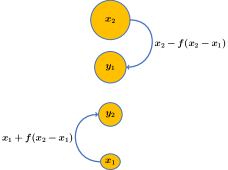
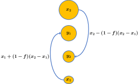
Figure 1: In the figure, a transfer between two individuals, and consider $x_{1}$ and $x_{2}$ (respectively $y_{1}$ and $y_{2}$) the values of the transferable quantities before transfer (respectively after transfer). We plot a transfer whenever $x_{2}>x_{1}$, and $f\in[0,1/2]$ (on the left hand side), and $(1-f)\in[1/2,1]$ (on the right hand side). We observe that the values $y_{1}$ and $y_{2}$ are the same on both sides.

In Figure 1, we use the following equalities

$$y_{1}=x_{2}-f(x_{2}-x_{1})=x_{1}+(1-f)(x_{2}-x_{1}),$$

and

$$y_{2}=x_{2}-(1-f)(x_{2}-x_{1})=x_{1}+(1-f)(x_{2}-x_{1}).$$

The values $y_{1}$ and $y_{2}$ are the same after a given transfer if we choose $f$ or $1-f$. In other words, we can not distinguish if $x_{1}$ and $x_{2}$ are ancestors of $y_{1}$ or $y_{2}$. This explains the mean value of Dirac masses in the kernel $K_{1}$. It follows, that this kind of kernel will preserve the support of the initial distribution, so we can restrict to any closed bounded interval $I\subset\mathbb{R}$. This transfer kernel corresponds to the one proposed to build the recombination operator in Magal and Webb [9]. An extended version with friction was proposed by Hinow, Le Foll, Magal, and Webb [6].

Here we can compute $B_{1}(u,v)$ explicitly when $I=\mathbb{R}$, $u\in L^{1}(\mathbb{R})$ and $v\in L^{1}(\mathbb{R})$. Indeed let $\varphi\in C_{c}(I)$ be a compactly supported test function. Then

$$\int_{\mathbb{R}}\varphi(x)B_{1}(u,v)(\mathrm{d}x) =\int_{x_{1}\in\mathbb{R}}\int_{x_{2}\in\mathbb{R}}\int_{x\in\mathbb{R}}\varphi(x)K_{1}(\mathrm{d}x,x_{1},x_{2})u(x_{1})\mathrm{d}x_{1}u(x_{2})\mathrm{d}x_{2}$$

$$=\iint_{\mathbb{R}\times\mathbb{R}}\frac{1}{2}\left(\varphi\big{(}x_{2}-f(x_{2}-x_{1})\big{)}+\varphi\big{(}x_{1}-f(x_{1}-x_{2})\big{)}\right)u(x_{1})v(x_{2})\mathrm{d}x_{1}\mathrm{d}x_{2}$$

$$=\frac{1}{2}\left(\iint_{\mathbb{R}\times\mathbb{R}}\varphi\big{(}(1-f)x_{2}+fx_{1}\big{)}u(x_{1})v(x_{2})\mathrm{d}x_{1}\mathrm{d}x_{2}\right.$$

$$\quad\left.+\iint_{\mathbb{R}\times\mathbb{R}}\varphi\big{(}(1-f)x_{1}+fx_{2}\big{)}u(x_{1})v(x_{2})\mathrm{d}x_{1}\mathrm{d}x_{2}\right)$$

$$=\frac{1}{2}\left(\iint_{\mathbb{R}\times\mathbb{R}}\varphi\big{(}(1-f)x_{2}+fx_{1}\big{)}u(x_{1})v(x_{2})\mathrm{d}x_{1}\mathrm{d}x_{2}\right.$$

$$\quad\left.+\iint_{\mathbb{R}\times\mathbb{R}}\varphi\big{(}(1-f)x_{2}+fx_{1}\big{)}u(x_{2})v(x_{1})\mathrm{d}x_{1}\mathrm{d}x_{2}\right).$$

Next, by using the change of variable

$$\left\{\begin{array}[]{l}x_{1}=x-(1-f)\sigma\\ x_{2}=x+f\sigma\end{array}\right.\Leftrightarrow\left\{\begin{array}[]{l}\sigma=x_{2}-x_{1}\\ x=(1-f)x_{2}+fx_{1}\end{array}\right.$$

we obtain

$$\int_{\mathbb{R}}\varphi(x)B_{1}(u,v)(\mathrm{d}x) =\frac{1}{2}\left(\int_{\mathbb{R}}\varphi\big{(}x\big{)}\int_{\mathbb{R}}u(x-(1-f)\sigma)v(x+f\sigma)\mathrm{d}\sigma\mathrm{d}x\right.$$

$$\quad\left.+\int_{\mathbb{R}}\varphi\big{(}x\big{)}\int_{\mathbb{R}}u(x+f\sigma)v(x-(1-f)\sigma)\mathrm{d}\sigma\mathrm{d}x\right),$$

and we obtain

$$B_{1}(u,v)(x)=\dfrac{1}{2}\left(\int_{\mathbb{R}}u(x-(1-f)\sigma)v\left(x+f\sigma\right)\mathrm{d}\sigma+\int_{\mathbb{R}}v(x-(1-f)\sigma)u\left(x+f\sigma\right)\mathrm{d}\sigma\right).$$

We conclude that the transfer operator restricted to $L^{1}_{+}(\mathbb{R})$ is defined by

$$T_{1}(u)(x)=\left\{\begin{array}[]{ll}\dfrac{\int_{\mathbb{R}}u(x-(1-f)\sigma)u\left(x+f\sigma\right)\mathrm{d}\sigma}{\int_{\mathbb{R}}u(x)\mathrm{d}x},\text{ if }u\in L^{1}_{+}(\mathbb{R})\setminus\left\{0\right\},\vspace{0.2cm}\\ 0,\text{ if }u=0.\end{array}\right.$$

Remark 2.1.

One may also consider the case where the fraction transferred varies in function of the distance between the poorest and richest before transferred. This problem was considered by Hinow, Le Foll, Magal and Webb [6], and in the case

$$K_{1}(\mathrm{d}x,x_{1},x_{2}):=\frac{1}{2}\left(\delta_{x_{2}-f(|x_{2}-x_{1}|)(x_{2}-x_{1})}(\mathrm{d}x)+\delta_{x_{1}-f(|x_{2}-x_{1}|)(x_{1}-x_{2})}(\mathrm{d}x)\right),$$

where $f:[0,+\infty)\to[0,1]$ is a continuous function.

2.2 Sheriff of Nottingham model: (the poorest give to the richest)

The poorest looses a fraction $f$ of the difference $|x_{2}-x_{1}|$, and the richest gains a fraction $f$ of the difference $|x_{2}-x_{1}|$

$$K_{2}(\mathrm{d}x,x_{1},x_{2}):=\frac{1}{2}\left(\delta_{x_{2}+f(x_{2}-x_{1})}(\mathrm{d}x)+\delta_{x_{1}+f(x_{1}-x_{2})}(\mathrm{d}x)\right),$$

where $f\in(0,1)$ is fixed.

This kind of kernel will expand the support of the initial distribution to the whole real line, therefore we can not restrict to bounded intervals $I\subset\mathbb{R}$.

In Figure 2, we explain why we need to consider a mean value of two Dirac masses in the kernel $K_{1}$. Indeed, we have

$$y_{2}=x_{2}+f(x_{2}-x_{1})=x_{1}+(1+f)(x_{2}-x_{1}),$$

and

$$y_{1}=x_{2}-(1+f)(x_{2}-x_{1})=x_{1}-f(x_{2}-x_{1}).$$

Therefore, the transferable quantities $y_{1}$ and $y_{2}$ after a given transfer, are the same with $f$ or $1+f$.

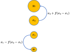
Figure 2: In the figure, the two values before transfers are $x_{1}$ and $x_{2}$, and the two values after transfer are $y_{1}$ and $y_{2}$. We plot a transfer whenever $x_{2}>x_{1}$, and $f\in[0,1]$ (on the left hand side), and $f$ is replaced by $1+f$ (on the right hand side). We observe that the values $y_{1}$ and $y_{2}$ are the same on both sides.

Here again we can compute $B_{2}(u,v)$ explicitly when $I=\mathbb{R}$, $u\in L^{1}(\mathbb{R})$ and $v\in L^{1}(\mathbb{R})$. Indeed let $\varphi\in C_{c}(I)$ be a compactly supported test function. Then

$$\int_{\mathbb{R}}\varphi(x)B_{2}(u,v)(\mathrm{d}x)$$

$$=\int_{x_{1}\in\mathbb{R}}\int_{x_{2}\in\mathbb{R}}\int_{x\in\mathbb{R}}\varphi(x)K_{2}(\mathrm{d}x,x_{1},x_{2})u(x_{1})\mathrm{d}x_{1}u(x_{2})\mathrm{d}x_{2}$$

$$=\iint_{\mathbb{R}\times\mathbb{R}}\frac{1}{2}\left(\varphi\big{(}x_{2}+f(x_{2}-x_{1})\big{)}+\varphi\big{(}x_{1}+f(x_{1}-x_{2})\big{)}\right)u(x_{1})v(x_{2})\mathrm{d}x_{1}\mathrm{d}x_{2}$$

$$=\frac{1}{2}\left(\iint_{\mathbb{R}\times\mathbb{R}}\varphi\big{(}(1+f)x_{2}-fx_{1}\big{)}u(x_{1})v(x_{2})\mathrm{d}x_{1}\mathrm{d}x_{2}\right.$$

$$\quad\left.+\iint_{\mathbb{R}\times\mathbb{R}}\varphi\big{(}(1+f)x_{1}-fx_{2}\big{)}u(x_{1})v(x_{2})\mathrm{d}x_{1}\mathrm{d}x_{2}\right)$$

$$=\frac{1}{2}\left(\iint_{\mathbb{R}\times\mathbb{R}}\varphi\big{(}(1+f)x_{2}-fx_{1}\big{)}u(x_{1})v(x_{2})\mathrm{d}x_{1}\mathrm{d}x_{2}\right.$$

$$\quad\left.+\iint_{\mathbb{R}\times\mathbb{R}}\varphi\big{(}(1+f)x_{2}-fx_{1}\big{)}u(x_{2})v(x_{1})\mathrm{d}x_{1}\mathrm{d}x_{2}\right).$$

Next, by using the change of variable

$$\left\{\begin{array}[]{l}x_{1}=x-(1+f)\sigma\\ x_{2}=x-f\sigma\end{array}\right.\Leftrightarrow\left\{\begin{array}[]{l}\sigma=x_{2}-x_{1}\\ x=(1+f)x_{2}-fx_{1}\end{array}\right.$$

we obtain

$$\int_{\mathbb{R}}\varphi(x)B_{2}(u,v)(\mathrm{d}x) =\frac{1}{2}\left(\int_{\mathbb{R}}\varphi\big{(}x\big{)}\int_{\mathbb{R}}u(x-(1+f)\sigma)v(x-f\sigma)\mathrm{d}\sigma\mathrm{d}x\right.$$

$$\quad\left.+\int_{\mathbb{R}}\varphi\big{(}x\big{)}\int_{\mathbb{R}}u(x-f\sigma)v(x-(1+f)\sigma)\mathrm{d}\sigma\mathrm{d}x\right),$$

and we obtain

$$B_{2}(u,v)(x)=\dfrac{1}{2}\left(\int_{\mathbb{R}}u(x-(1+f)\sigma)v\left(x-f\sigma\right)\mathrm{d}\sigma+\int_{\mathbb{R}}v(x-(1+f)\sigma)u\left(x-f\sigma\right)\mathrm{d}\sigma\right).$$

We conclude that the transfer operator restricted to $L^{1}_{+}(\mathbb{R})$ is defined by

$$T_{2}(u)(x)=\left\{\begin{array}[]{ll}\dfrac{\int_{\mathbb{R}}u(x-(1+f)\sigma)u\left(x-f\sigma\right)\mathrm{d}\sigma}{\int_{\mathbb{R}}u(x)\mathrm{d}x},\text{ if }u\in L^{1}_{+}(\mathbb{R})\setminus\left\{0\right\},\vspace{0.2cm}\\ 0,\text{ if }u=0.\end{array}\right.$$

3 Understanding (1.1) in the space of measures

Before anything, we need to define $B(u,v)(dx)$ whenever $u$ and $v$ are finite measures on $I$.

Theorem 3.1.

Let Assumption 1.1 be satisfied. Define

$$B(u,v)(A):=\iint_{I^{2}}K(A,x_{1},x_{2})u(\mathrm{d}x_{1})v(\mathrm{d}x_{2}),$$ (3.1)

for each Borel set $A\subset I$, and each $u,v\in\mathcal{M}(I)$.

Then $B$ maps $\mathcal{M}(I)\times\mathcal{M}(I)$ into $\mathcal{M}(I)$, and satisfies the following properties

• $$\|B(u,v)\|_{\mathcal{M}(I)}\leq\|u\|_{\mathcal{M}(I)}\|v\|_{\mathcal{M}(I)},\forall u,v\in\mathcal{M}(I).$$

• $$B(u,v)\in M_{+}(I),\forall u,v\in M_{+}(I),$$

• $$\int_{I}B(u,v)(\mathrm{d}x)=\int_{I}u(\mathrm{d}x_{1})\int_{I}v(\mathrm{d}x_{2}),\forall u,v\in M_{+}(I).$$

• $$\int_{I}xB(u,v)(\mathrm{d}x)=\dfrac{\int_{I}x_{1}u(\mathrm{d}x_{1})\int_{I}v(\mathrm{d}x_{2})+\int_{I}u(\mathrm{d}x)\int_{I}x_{2}v(\mathrm{d}x_{2})}{2},\forall u,v\in M_{+}(I).$$

• For each integer $n\geq 0$,

  $$\int_{I}x^{n}B(u,v)(dx)=\int_{I\times I}\int_{I}x^{n}K(dx,x_{1},x_{2})\,u(dx_{1})\,v(dx_{2}),\forall u,v\in M_{+}(I).$$

Proof.

Let $u\in\mathcal{M}(I)$, $v\in\mathcal{M}(I)$ and define

$$w(\mathrm{d}x):=B(u,v)(\mathrm{d}x)$$

by (3.1). Let $(A_{n})_{n\in\mathbb{N}}$ a collection of pairwise disjoint Borel-measurable sets in $I$. We want to prove that

$$w\left(\bigcup_{n\in\mathbb{N}}A_{n}\right) =\sum_{n\in\mathbb{N}}w(A_{n}).$$ (3.2)

We have

$$\begin{array}[]{ll}w\left(\bigcup_{n\in\mathbb{N}}A_{n}\right)&=\displaystyle\iint_{I^{2}}K\left(\bigcup_{n\in\mathbb{N}}A_{n},x_{1},x_{2}\right)u(\mathrm{d}x_{1})v(\mathrm{d}x_{2})\\ &=\displaystyle\iint_{I^{2}}\sum_{n\in\mathbb{N}}K(A_{n},x_{1},x_{2})u(\mathrm{d}x_{1})v(\mathrm{d}x_{2}).\end{array}$$

In order to change the order of summation between the integral and the sum, we will use Fubini’s Theorem [4, Vol. I Theorem 3.4.4 p.185] and Tonnelli’s Theorem [4, Vol. I Theorem 3.4.5 p.185].

We consider $P\subset\mathcal{B}(I^{2})$ the support of the positive part of $u\otimes v$ (as given by [4, Theorem 3.1.1 p. 175]). That is

$$\mathbbm{1}_{P}u\otimes v\in M_{+}(I^{2}),\text{ and }-\mathbbm{1}_{P^{c}}u\otimes v\in M_{+}(I^{2}),$$

where $\mathbbm{1}_{P}$ (respectively $\mathbbm{1}_{P^{c}}$) is the indicator functions of $P$, that is $\mathbbm{1}_{P}(x)=1$ if $x\in P$ else $\mathbbm{1}_{P}(x)=0$ (respectively the indicator function of $P^{c}=I\setminus P$ the complement set of $P$).

We consider the maps defined for all $n\in\mathbb{N}$, and all $x_{1},x_{2}\in I,$

$$f_{n}(x_{1},x_{2}):=\mathbbm{1}_{P}K(A_{n},x_{1},x_{2}),$$ (3.3)

and

$$\,f(n,x_{1},x_{2}):=f_{n}(x_{1},x_{2}).$$

Then by Assumption 1.1-(i), for each integer $n\in\mathbb{N}$ the map $f_{n}$ is Borel measurable (i.e., measurable with respect to the Borel $\sigma$-algebra), and for each Borel set $B\subset\mathbb{R}$, we have

$$f^{-1}(B)=\bigcup_{n\in\mathbb{N}}\{n\}\times f_{n}^{-1}(B).$$

Consequently, $f$ is measurable for the $\sigma$-algebra $\mathcal{P}(\mathbb{N})\otimes\mathcal{B}(I^{2})$, the smallest $\sigma$-algebra in $\mathcal{P}(\mathbb{N}\times I^{2})$ that contains all rectangles $\mathcal{N}\times B$ where $\mathcal{N}\in\mathcal{P}(\mathbb{N})$ and $B\in\mathcal{B}(I^{2})$.

Let $c$ be the counting measure on $\mathbb{N}$, $c:=\sum_{n\in\mathbb{N}}\delta_{n}$. By Tonnelli’s Theorem [4, Vol. I Theorem 3.4.5 p.185], since $f$ is nonnegative, and $c$ and $(u\otimes v)_{+}$ are nonnegative $\sigma$-finite measures, and

$$\int_{I^{2}}\int_{\mathbb{N}}f(n,x_{1},x_{2})c(\mathrm{d}n)(u\otimes v)_{+}(\mathrm{d}x_{1}\mathrm{d}x_{2})$$

$$=\int_{I^{2}}\sum_{n\in\mathbb{N}}\mathbbm{1}_{P}(x_{1},x_{2})K(A_{n},x_{1},x_{2})(u\otimes v)_{+}(\mathrm{d}x_{1}\mathrm{d}x_{2})$$

$$=\iint_{I^{2}}\mathbbm{1}_{P}(x_{1},x_{2})K\left(\bigcup_{n\in\mathbb{N}}A_{n},x_{1},x_{2}\right)u(\mathrm{d}x_{1})v(\mathrm{d}x_{2})$$

$$\leq\iint_{I^{2}}\mathbbm{1}_{P}(x_{1},x_{2})K\left(I^{2},x_{1},x_{2}\right)u(\mathrm{d}x_{1})v(\mathrm{d}x_{2})$$

$$=(u\otimes v)(P)<+\infty.$$

We conclude that $f\in L^{1}(c\otimes(u\otimes v)_{+})$ and therefore by Fubini’s Theorem [4, Vol. I Theorem 3.4.4 p.185] we have

$$\int_{I^{2}}\int_{\mathbb{N}}f(n,x_{1},x_{2})c(\mathrm{d}n)(u\otimes v)_{+}(\mathrm{d}x_{1}\mathrm{d}x_{2})$$

$$=\int_{\mathbb{N}}\int_{I^{2}}f(n,x_{1},x_{2})c(\mathrm{d}n)(u\otimes v)_{+}(\mathrm{d}x_{1}\mathrm{d}x_{2}).$$

This means that

$$\iint_{I^{2}}\sum_{n\in\mathbb{N}}\mathbbm{1}_{P}K(A_{n},x_{1},x_{2})u(\mathrm{d}x_{1})v(\mathrm{d}x_{2})$$

$$=\sum_{n\in\mathbb{N}}\iint_{I^{2}}\mathbbm{1}_{P}K(A_{n},x_{1},x_{2})u(\mathrm{d}x_{1})v(\mathrm{d}x_{2}).$$

By similar arguments we can show that

$$\iint_{I^{2}}\sum_{n\in\mathbb{N}}(-\mathbbm{1}_{P^{c}})K(A_{n},x_{1},x_{2})u(\mathrm{d}x_{1})v(\mathrm{d}x_{2})$$

$$=\sum_{n\in\mathbb{N}}\iint_{I^{2}}(-\mathbbm{1}_{P^{c}})K(A_{n},x_{1},x_{2})u(\mathrm{d}x_{1})v(\mathrm{d}x_{2}).$$

We conclude that

$$\iint_{I^{2}}\sum_{n\in\mathbb{N}}K(A_{n},x_{1},x_{2})u(\mathrm{d}x_{1})v(\mathrm{d}x_{2})$$

$$=\iint_{I^{2}}\sum_{n\in\mathbb{N}}(\mathbbm{1}_{P}+\mathbbm{1}_{P^{c}})K(A_{n},x_{1},x_{2})u(\mathrm{d}x_{1})v(\mathrm{d}x_{2})$$

$$=\iint_{I^{2}}\sum_{n\in\mathbb{N}}\mathbbm{1}_{P}K(A_{n},x_{1},x_{2})u(\mathrm{d}x_{1})v(\mathrm{d}x_{2})$$

$$\quad+\iint_{I^{2}}\sum_{n\in\mathbb{N}}\mathbbm{1}_{P^{c}}K(A_{n},x_{1},x_{2})u(\mathrm{d}x_{1})v(\mathrm{d}x_{2})$$

$$=\sum_{n\in\mathbb{N}}\iint_{I^{2}}\mathbbm{1}_{P}K(A_{n},x_{1},x_{2})u(\mathrm{d}x_{1})v(\mathrm{d}x_{2})$$

$$\quad+\sum_{n\in\mathbb{N}}\iint_{I^{2}}\mathbbm{1}_{P^{c}}K(A_{n},x_{1},x_{2})u(\mathrm{d}x_{1})v(\mathrm{d}x_{2})$$

$$=\sum_{n\in\mathbb{N}}\iint_{I^{2}}K(A_{n},x_{1},x_{2})u(\mathrm{d}x_{1})v(\mathrm{d}x_{2})$$

$$=\sum_{n\in\mathbb{N}}w(A_{n}).$$

We have proved (3.2) for any family of pairwise disjoint Borel sets $(A_{n})$, hence $w$ is a measure. Moreover $w$ is finite because

$$\int_{I}|w|(\mathrm{d}x)=|w|(I) \leq\iint_{I^{2}}K(I,x_{1},x_{2})|u\otimes v|(\mathrm{d}x_{1}\mathrm{d}x_{2})$$

$$=\iint_{I^{2}}|u|(\mathrm{d}x_{1})|v|(\mathrm{d}x_{2})$$

$$=\|u\|_{\mathcal{M}(I)}\|v\|_{\mathcal{M}(I)}.$$

We have proved that

$$\|B(u,v)\|_{\mathcal{M}(I)}\leq\|u\|_{\mathcal{M}(I)}\|v\|_{\mathcal{M}(I)}.$$

Hence $B(u,v)$ is a continuous bilinear map on $\mathcal{M}(X)$.

To prove (iii), we use Fubini’s theorem in the formula (3.1) of $B(u,v)$. To prove (iv), we use the definition (3.1) of $B(u,v)$:

$$\begin{array}[]{ll}\int_{I}B(u,v)(\mathrm{d}x)=B(u,v)(I)&=\iint_{I^{2}}K(I,x_{1},x_{2})u(\mathrm{d}x_{1})v(\mathrm{d}x_{2})\\ &=\iint_{I^{2}}u(\mathrm{d}x_{1})v(\mathrm{d}x_{2})\\ &=\int_{I}u(\mathrm{d}x)\int_{I}v(\mathrm{d}x),\end{array}$$

because $K(I,x_{1},x_{2})=1$ by assumption.

To prove (v), we use Fubini’s theorem applied to the formula (3.1) of $B(u,v)$:

$$\begin{array}[]{ll}\int_{I}xB(u,v)(\mathrm{d}x)&=\iint_{I^{2}}\int_{I}xK(dx,x_{1},x_{2})u(\mathrm{d}x_{1})v(\mathrm{d}x_{2})\\ &=\iint_{I^{2}}\dfrac{x_{1}+x_{2}}{2}u(\mathrm{d}x_{1})v(\mathrm{d}x_{2})\\ &=\dfrac{\int_{I}x_{1}u(\mathrm{d}x_{1})\int_{I}v(\mathrm{d}x_{2})+\int_{I}u(\mathrm{d}x_{1})\int_{I}x_{2}v(\mathrm{d}x_{2})}{2},\end{array}$$

because $\int_{I}xK(dx,x_{1},x_{2})=\dfrac{x_{1}+x_{2}}{2}$ by assumption. ∎

As a consequence of Theorem 3.1, the map $B$ is a bounded and bi-linear operator from $\mathcal{M}(I)\times\mathcal{M}(I)$ to $\mathcal{M}(I)$. Moreover $B$ maps $M_{+}(I)\times M_{+}(I)$ into $M_{+}(I)$. To investigate the Lipschitz property of $T:M_{+}(I)\to M_{+}(I)$, it is sufficient to observe that (here for short we replace $\|.\|_{\mathcal{M}(I)}$ by $\|.\|$)

$$\begin{array}[]{ll}\|T(u)-T(v)\|\\ =\bigg{\|}\|u\|^{-1}B(u,u-v)+\left(\|u\|^{-1}-\|v\|^{-1}\right)B(u,v)+\|v\|^{-1}B(u-v,v)\bigg{\|}\vspace{0.2cm}\\ \leq\bigg{\|}\|u\|^{-1}B(u,|u-v|)+\left(\|u\|^{-1}-\|v\|^{-1}\right)B(u,v)+\|v\|^{-1}B(|u-v|,v)\bigg{\|}\vspace{0.2cm}\\ \leq 2\,\|u-v\|+|\|u\|^{-1}-\|v\|^{-1}|\,\|u\|\,\|v\|\vspace{0.2cm}\\ \leq 2\,\|u-v\|+|\|u\|-\|v\||\vspace{0.2cm}\\ \leq 3\,\|u-v\|,\end{array}$$

therefore we obtain the following proposition.

Proposition 3.2.

Let Assumption 1.1 be satisfied. The operator $T$ map $M_{+}(I)$ into itself, and $T$ satisfies the following properties

• $T:M_{+}(I)\to M_{+}(I)$ is Lipchitz continuous.

• $T$ is positively homogeneous. That is,

  $$T(\lambda u)=\lambda T(u),\forall\lambda\geq 0,\forall u\in M_{+}(I).$$

• $T$ preserves the total mass of individuals. That is,

  $$\int_{I}T(u)(dx)=\int_{I}u(dx),\forall u\in M_{+}(I).$$

• $T$ preserves the total mass of transferable quantity. That is,

  $$\int_{I}xT(u)(dx)=\int_{I}xu(dx),\forall u\in M_{+}(I).$$

Therefore we obtain the following theorem.

Theorem 3.3.

Let Assumption 1.1 be satisfied. Then the Cauchy problem is

$$\partial_{t}u(t,dx)=2\tau\,T\big{(}u(t)\big{)}(dx)-2\tau\,u(t,dx),$$ (3.4)

with

$$u(0,dx)=\phi(dx)\in M_{+}(I).$$ (3.5)

The Cauchy problem generates a unique continuous homogeneous semiflow $t\to S(t)\phi$ on $M_{+}(I)$. That is

• (Semiflow property)

  $$S(0)\phi=\phi\text{ and }S(t)S(s)\phi=S(t+s)\phi,\forall t,s\geq 0,\forall\phi\in M_{+}(I).$$

• (Continuity) The map $(t,\phi)\to S(t)\phi$ is a continuous map from $[0,+\infty)\times M_{+}(I)$ to $M_{+}(I)$.

• (Homogeneity)

  $$S(t)\lambda\phi=\lambda S(t)\phi,\forall t\geq 0,\forall\lambda\geq 0,\forall\phi\in M_{+}(I).$$

• (Preservation of the total mass of individuals) The total mass of individuals is preserved

  $$\int_{I}S(t)(\phi)(dx)=\int_{I}\phi(dx),\forall t\geq 0,\forall\lambda\geq 0,\forall\phi\in M_{+}(I).$$

• (Preservation of the total mass of transferable quantity) The total mass of transferable quantity is preserved

  $$\int_{I}xS(t)(\phi)(dx)=\int_{I}x\phi(dx),\forall t\geq 0,\forall\lambda\geq 0,\forall\phi\in M_{+}(I).$$

• (From transfer rate $1/2$ to any transfer rate $\tau>0$) If we define $S^{\star}(t)$ the semi-flow generated by (3.4)-(3.5) whenever $\tau=1/2$, then

  $$S(t)=S^{\star}\left(2\tau t\right),\forall t\geq 0.$$

Remark 3.4.

Let $\mathcal{F}:\mathcal{M}(I)\to\mathbb{R}$ be a positive bounded linear form on $\mathcal{M}(I)$. We can consider for example

$$\mathcal{F}(u)=\int_{I}f(x)u(dx),$$

where $f:I\to\mathbb{R}$ a bounded and positive continuous map on $I$.

Then $(t,\phi)\mapsto U(t)\phi$ define on $[0,+\infty)\times M_{+}(I)$ by

$$U(t)u=\dfrac{S(t)\phi}{1+\int_{0}^{t}\mathcal{F}(S(\sigma)\phi)d\sigma},$$

is the unique solution of the Cauchy problem

$$u^{\prime}(t)=2\tau\,T\big{(}|u(t)|\big{)}(dx)-2\tau\,u(t,dx)-\mathcal{F}(u(t))u(t,dx),$$

with

$$u(0,dx)=\phi(dx)\in M_{+}(I).$$

More detailed arguments can be found in Magal and Webb [9], and Magal [7].

Remark 3.5.

The rate of transfers $\tau(x)$ may vary in function of $x$ the transferable quantity. In that case, we obtain the following model

$$\partial_{t}u(t,x)=T\big{(}2\tau(.)\,u(t,.)\big{)}(x)-2\tau(x)u(t,x),\text{ for }x\in\mathbb{R},$$

with

$$u(0,dx)=\phi(dx)\in\mathcal{M}(I).$$

4 Understanding (1.1) in $L^{1}(\mathbb{R})$

Recall that a Borel subset $A\in\mathcal{B}(I)$ is said to be negligible if and only if $A$ has a null Lebesgue measure. Then, thanks to the Radon-Nikodym Theorem A.6, we have the following characterization of kernels that define a bilinear mapping from $L^{1}(I)\times L^{1}(I)$ to $L^{1}(I)$.

Proposition 4.1.

Let Assumption 1.1 be satisfied. Then we have

$$B(u,v)\in L^{1}(I)\text{ for all }(u,v)\in L^{1}(I)\times L^{1}(I)$$

if, and only if, for each negligible subset $A\in\mathcal{B}(I)$, the set

$$\mathcal{N}(A):=\left\{(x_{1},x_{2})\in I\times I\,:\,K(A,x_{1},x_{2})\neq 0\right\},$$

is negligible. Equivalently, we have

$$\iint_{I\times I}K(A,x_{1},x_{2})\mathrm{d}x_{1}\mathrm{d}x_{2}=0,$$

whenever $A\in\mathcal{B}(I)$ is negligible.

Proof.

For simplicity, here we call $\mathcal{L}$ the one-dimensional Lebesgue measure, that is to say $\mathcal{L}(A)=\int_{A}\mathrm{d}x$; and $\mathcal{L}^{2}:=\mathcal{L}\otimes\mathcal{L}$ the two-dimensional Lebesgue measure in $\mathbb{R}^{2}$.

Let $u,v\in L^{1}(I)$ be given. Suppose that

$$\mathcal{L}^{2}(\mathcal{N}(A))=0,$$

for each $A\in\mathcal{B}(I)$ with $\mathcal{L}(A)=0$. Then by definition (see (3.1)),

$$B(u,v)(A)=\iint_{I\times I}K(A,x_{1},x_{2})u(x_{1})\mathrm{d}x_{1}v(x_{2})\mathrm{d}x_{2}=0,$$

since $(x_{1},x_{2})\mapsto K(A,x_{1},x_{2})$ is equal to zero $\mathcal{L}^{2}$-almost everywhere in $\mathbb{R}^{2}$ by assumption. Therefore $B(u,v)$ is absolutely continuous with respect to the Lebesgue measure $\mathcal{L}$, and by the Radon-Nikodym Theorem A.6, we can find function $f\in L^{1}(I)$ such that

$$B(u,v)(dx)=f(x)\mathrm{d}x,$$

which is equivalent to

$$B(u,v)\in L^{1}(I).$$

Conversely, assume that $B(u,v)\in L^{1}(I)$ for any $(u,v)\in L^{1}(I)^{2}$. If $I$ is bounded then $1\in L^{1}(I)$, so taking $u=v=1$, and $B(1,1)(\mathrm{d}x)=f(x)\mathrm{d}x$ with $f\in L^{1}(I)$ gives

$$B(u,v)(A)=\iint_{I\times I}K(A,x_{1},x_{2})\mathrm{d}x_{1}\mathrm{d}x_{2}=\int_{A}f(x)\mathrm{d}x=0,$$

whenever $\mathcal{L}(A)=0$, and we are done.

Let us consider the case when $I$ is not bounded. Assume that $A\in\mathcal{B}(I)$ is negligible. Define

$$u_{n}(x)=v_{n}(x)=\mathbbm{1}_{[-n,n]\cap I}(x)$$

where $x\mapsto\mathbbm{1}_{E}(x)$ is the indicator function of the set $E$.

Then, we have by assumption,

$$B(u_{n},v_{n})=f_{n}(x)\mathrm{d}x$$

for some $f_{n}\in L^{1}(I)$.

Moreover

$$B\big{(}u_{n},v_{n}\big{)}(A)=\iint_{(I\cap[-n,n])\times(I\cap[-n,n])}K(A,x_{1},x_{2})\mathrm{d}x_{1}\mathrm{d}x_{2}=\int_{A}f_{n}(x)\mathrm{d}x=0,$$

thus

$$\mathcal{L}\big{(}\mathcal{N}(A)\cap[-n,n]^{2}\big{)}=0\text{ for all }n\in\mathbb{N}.$$

Finally since we have an increase sequence of subsets, we obtain

$$\mathcal{L}\big{(}\mathcal{N}(A)\big{)}=\mathcal{L}\left(\mathcal{N}(A)\cap\bigcup_{n\in\mathbb{N}}[-n,n]^{2}\right)=\lim_{n\to+\infty}\mathcal{L}\left(\mathcal{N}(A)\cap[-n,n]^{2}\right)=0,$$

and the proof is completed. ∎

Since the norm in measure coincides with the $L^{1}$ for an $L^{1}$ function, we deduce that $T$ maps $L^{1}_{+}(I)$ into $L^{1}_{+}(I)$ into itself, and the following statements are consequences of Theorem 3.3, and Proposition 4.1.

Theorem 4.2.

Let Assumption 1.1 be satisfied. Then the Cauchy problem is

$$\partial_{t}u(t,x)=2\tau\,T\big{(}u(t)\big{)}-2\tau\,u(t,x),$$ (4.1)

with

$$u(0,x)=\phi(x)\in L^{1}_{+}(I).$$ (4.2)

The Cauchy problem (4.1)-(4.2), generates a unique semiflow which is the restriction of $S(t)$ to $L^{1}_{+}(I)$. We deduce that

$$S(t)L^{1}_{+}(I)\subset L^{1}_{+}(I),\forall t\geq 0,$$

and the semiflow $t\to S(t)\phi$ restricted to $L^{1}_{+}(I)$ satisfies the following properties:

• (Continuity) The map $(t,\phi)\to S(t)\phi$ is a continuous map from $[0,+\infty)\times L^{1}_{+}(I)$ to $L^{1}_{+}(I)$.

• (Preservation of the total mass of individuals) The total mass of individuals is preserved

  $$\int_{I}S(t)(\phi)(x)dx=\int_{I}\phi(x)dx,\forall t\geq 0,\forall\lambda\geq 0,\forall\phi\in M_{+}(I).$$

• (Preservation of the total mass of transferable quantity) The total mass of transferable quantity is preserved

  $$\int_{I}xS(t)(\phi)(x)dx=\int_{I}x\phi(x)dx,\forall t\geq 0,\forall\lambda\geq 0,\forall\phi\in M_{+}(I).$$

Example 4.3 (Robin Hood model).

Let $K(\mathrm{d}x,x_{1},x_{2})=K_{1}(\mathrm{d}x,x_{1},x_{2})=\frac{1}{2}\big{(}\delta_{x_{2}-f(x_{2}-x_{1})}(\mathrm{d}x)+\delta_{x_{1}-f(x_{1}-x_{2})}(\mathrm{d}x)\big{)}$. If $A\in\mathcal{B}(I)$ has zero Lebesgue measure, then we have:

$$\mathcal{N}(A) =\{(x_{1},x_{2})\in I\times I\,:\,K(A,x_{1},x_{2})>0\}$$

$$=\{(x_{1},x_{2})\,:\,x_{2}-f(x_{2}-x_{1})=y\in A\text{ or }x_{1}-f(x_{1}-x_{2})=z\in A\}$$

$$=\left\{(x_{1},x_{2})\,:\,x_{1}=\frac{1-f}{1-2f}z-\frac{f}{1-2f}y\text{ and }\right.$$

$$\hskip 28.45274pt\left.x_{2}=\frac{1-f}{1-2f}y-\frac{f}{1-2f}z\text{ and }\big{(}y\in A\text{ or }z\in A\big{)}\right\}$$

$$=\left\{\left(\frac{1-f}{1-2f}z-\frac{f}{1-2f}y,\frac{1-f}{1-2f}y-\frac{f}{1-2f}z\right)\,:\,y\in A,z\in I\right\}$$

$$\quad\cup\left\{\left(\frac{1-f}{1-2f}z-\frac{f}{1-2f}y,\frac{1-f}{1-2f}y-\frac{f}{1-2f}z\right)\,:\,y\in I,z\in A\right\}.$$

The two sets above have zero Lebesgue measure because they are the image of $A\times I$ and $I\times A$ by a linear invertible transformation. Therefore $\mathcal{N}(A)$ has zero Lebesgue measure and we can apply Proposition 4.1.

Example 4.4 (Sheriff of Nottingham model).

Let $K(\mathrm{d}x,x_{1},x_{2})=K_{2}(\mathrm{d}x,x_{1},x_{2})=\frac{1}{2}\big{(}\delta_{x_{2}+f(x_{2}-x_{1})}(\mathrm{d}x)+\delta_{x_{1}+f(x_{1}-x_{2})}(\mathrm{d}x)\big{)}$. If $A\in\mathcal{B}(\mathbb{R})$ has zero Lebesgue measure, then we have:

$$\mathcal{N}(A) =\{(x_{1},x_{2})\in I\times I\,:\,K(A,x_{1},x_{2})>0\}$$

$$=\{(x_{1},x_{2})\,:\,x_{2}+f(x_{2}-x_{1})=y\in A\text{ or }x_{1}+f(x_{1}-x_{2})=z\in A\}$$

$$=\left\{\left(\frac{1+f}{1+2f}z+\frac{f}{1+2f}y,\frac{1+f}{1+2f}y+\frac{f}{1+2f}z\right)\,:\,y\in A,z\in I\right\}$$

$$\quad\cup\left\{\left(\frac{1+f}{1+2f}z+\frac{f}{1+2f}y,\frac{1+f}{1+2f}y+\frac{f}{1+2f}z\right)\,:\,y\in I,z\in A\right\}.$$

The two sets above have zero Lebesgue measure because they are the image of $A\times\mathbb{R}$ and $\mathbb{R}\times A$ by a linear invertible transformation. Therefore $\mathcal{N}(A)$ has zero Lebesgue measure and we can apply Proposition 4.1.

Similarly, the mixed Robin Hood and Sheriff of Nottingham model also define a bilinear mapping from $L^{1}\times L^{1}$ to $L^{1}$.

Example 4.5 (Distributed Robin Hood or Sheriff of Nottingham models).

The kernel of the distributed Robin Hood model consists in replacing the Dirac mass centered a $0$, by $x\to g(x)\in L^{1}(I)$ a density of probability centered at $0$. That is

$$K_{3}(\mathrm{d}x,x_{1},x_{2})=\frac{1}{2}\bigg{\{}g\left(x-\left[x_{2}-f(x_{2}-x_{1})\right]\right)+g\left(x-\left[x_{1}-f(x_{1}-x_{2})\right]\right)\bigg{\}}\,\mathrm{d}x.$$

Similarly, the kernel of the distributed Sheriff of Nottingham model is the following

$$K_{4}(\mathrm{d}x,x_{1},x_{2}):=\frac{1}{2}\bigg{\{}g\left(x-\left[x_{2}+f(x_{2}-x_{1})\right]\right)+g\left(x-\left[x_{1}+f(x_{1}-x_{2})\right]\right)\bigg{\}}\,\mathrm{d}x.$$

Let $K(\mathrm{d}x,x_{1},x_{2})=K(x,x_{1},x_{2})\mathrm{d}x$ with $K(x,x_{1},x_{2})\in L^{1}(I)$ for any $(x_{1},x_{2})\in I\times I$. Examples are the distributed Robin Hood model, distributed Sheriff of Nottingham model, and distributed mixed Robin Hood and Sheriff of Nottingham model. If $A\in\mathcal{B}(I)$ has zero Lebesgue measure, then we have automatically

$$K(A,x_{1},x_{2})=\int_{A}K(x,x_{1},x_{2})\mathrm{d}x=0\text{ for any }(x_{1},x_{2})\in I\times I,\text{ so }\mathcal{N}(A)=\varnothing.$$

Therefore we can apply Proposition 4.1.

5 Numerical simulation

We introduce $p\in[0,1]$, the population’s redistribution fraction. The parameter $p$ is also the probability of applying the Robin Hood (RH) model during a transfer between two individuals. Otherwise, we use the Sheriff of Nottingham (SN) model with the probability $1-p$. In that case, the model is the following

$$\partial_{t}u(t,dx)=2\tau\,\left[p\,T_{1}\big{(}u(t)\big{)}(dx)+(1-p)\,T_{2}\big{(}u(t)\big{)}(dx)\right]-2\tau\,u(t,dx),$$ (5.1)

with

$$u(0,dx)=\phi(dx)\in M_{+}(I).$$ (5.2)

In Figures 3-7, we run an individual based simulation of the model (5.1)-(5.2). Such simulations are stochastic. We first choose a pair randomly following an exponential law with average $1/\tau$. Then we choose the RH model with a probability $p$ and the SN model with a probability $1-p$. Then we apply the transfers rule described in section 2. To connect this problem with our description in the space of measures, we can consider an initial distribution that is a sum of Dirac masses.

$$\phi(dx)=\sum_{i=1}^{N}\delta_{x_{i}}(x),$$

in which $x_{i}$ is the value of the transferable quantity for individual $i$ at $t=0$.

(a)                                             (b)
         

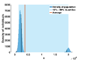
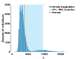
(c)                                             (d)
         

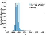
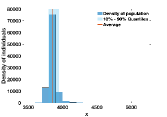
Figure 3: In this figure, we use $p=1$ (i.e. $100\%$ RH model), $f_{1}=f_{2}=0.1$, $1/\tau=1$ years. We start the simulations with $100\,000$ individuals. The figures (a) (b) (c) (d) are respectively the initial distribution at time $t=0$, and the distribution $10$ years, $50$ years and $100$ years.

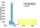
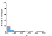
Figure 4: In this figure, we zoom on the distribution for $t=100$ in Figure 3 (d). The figure on the right-hand side corresponds to the yellow region in the left figure.

(a)                                             (b)
         

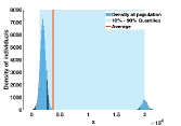
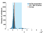
(c)                                             (d)
         

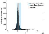
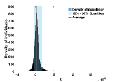
Figure 5: In this figure, we use $p=0.5$ (i.e. $50\%$ RH model and $50\%$ SN model), $f_{1}=f_{2}=0.1$, $1/\tau=1$ years. We start the simulations with $100\,000$ individuals. The figures (a) (b) (c) (d) are respectively the initial distribution at time $t=0$, and the distribution $10$ years, $50$ years and $100$ years.

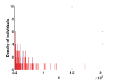
Figure 6: In this figure, we zoom on the distribution for $t=100$ in Figure 5 (d). The figure on the right-hand side corresponds to the yellow region in the left figure.

(a)                                             (b)
         

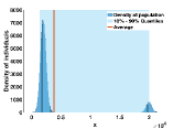
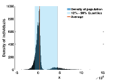
(c)                                             (d)
         

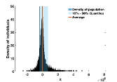
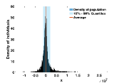
Figure 7: In this figure, we use $p=0$ (i.e. $0\%$ RH model and $100\%$ SN model), $f_{1}=f_{2}=0.1$, $1/\tau=1$ years. We start the simulations with $100\,000$ individuals. The figures (a) (b) (c) (d) are respectively the initial distribution at time $t=0$, and the distribution $10$ years, $50$ years and $100$ years.

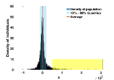
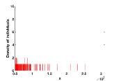
Figure 8: In this figure, we zoom on the distribution for $t=100$ in Figure 7 (d). The figure on the right-hand side corresponds to the yellow region in the left figure.

Figure 3 corresponds to the full RH model which corresponds to $p=1$. In that case, the population density converges to a Dirac mass centered at the mean value. That is, everyone will ultimately have the same amount of transferable quantity.

Whatever the value of $p$ strictly less than $1$, the simulations can be summed up by saying that "there is always a sheriff in town". In Figures 5-7, the unit for $x$-axis changes from (a) to (d). We can see from that some rich guys will always become richer and richer. The SN model induces competition between the poorest individuals also, and the population ends up after 100 years with a lot of debts. In other words, the richest individuals are becoming richer, while the poorest are becoming poorer. The effect in changing the value of the parameter $p\in[0,1)$ is strictly positive, it seems that it is only a matter of time before we end up with a very segregated population. We observe a difference for the richest of two orders of magnitude between the case $p=0.5$ and $p=0$. We conclude by observing that the smaller $p$ is, the more the wealthiest individuals are rich.

Appendix

Appendix A Spaces of measures

Let $X$ be a Polish space, that is complete metric space $(X,d)$ which is separable (i.e., there exists a countable dense subset). As an example for $X$ one may consider any closed subset of $\mathbb{R}^{n}$ endowed with the standard metric $d(x,y)=\|x-y\|$ induced by $\|.\|$ a norm on $\mathbb{R}^{n}$.

Recall that the Borel $\sigma$-algebra of $X$ is the set $\mathcal{B}(X)\subset\mathcal{P}(X)$ (the $\sigma$-algebra generated by the open subsets of $X$) of all parts of $X$ that can be obtained by countable union, countable intersection, and difference of open sets [4, Vol II Chap 6 section 6.3].

We define $\mathcal{M}(X)$ the space of measures on $X$ starting with the positive measures. A map $\mu:\mathcal{B}(X)\to\mathbb{R}^{+}$ is a positive measure, if it is additive (or a countably additive). That is,

$$\mu\left(\bigcup_{n\in\mathbb{N}}B_{n}\right)=\sum_{n\in\mathbb{N}}\mu(B_{n}),$$

for any countable collection of disjoint Borel sets $B_{n}\in\mathcal{B}(X)$ (where the empty set may occur infinitely many times). In the following, a countably additive measure will be called Borel measure.

A positive measure is finite if

$$\mu(X)<+\infty.$$

A signed measure $\mu$ is the difference between two positive measures

$$\mu=\mu^{+}-\mu^{-}$$

where $\mu^{+}$ and $\mu^{-}$ are both positive finite measures.

Definition A.1.

The set $\mathcal{M}(X)$ is the space of all the signed finite measures $\mu$.

Given a signed measure $\mu$, the Hahn decomposition theorem [4, Vol. I Theorem 3.1.1 p. 175] gives a decomposition of the space $X$ into two subsets $X^{+}$ and $X^{-}$ on which $\mu$ has constant sign.

Theorem A.2 (Hahn decomposition).

Let $\mu$ be a signed measure on a measurable space $(X,\mathcal{B}(X))$. Then, there exist disjoint sets $X^{+},X^{-}\in\mathcal{B}(X)$ such that $X^{+}\cup X^{-}=X,$ and for all $A\in\mathcal{B}(X)$, one has

$$\mu(A\cap X^{-})\leq 0\text{ and }\mu(A\cap X^{+})\geq 0.$$

Considering for example $\mu=\delta_{0}-\delta_{2}$ with $X=\{0,1,2\}$, we deduce that the Hahn decomposition is not unique in general. But the Hahn decomposition allows us to define the positive part $\mu^{+}$ and the negative part $\mu^{-}$ of a signed measure $\mu$:

$$\mu^{-}(A):=-\mu(A\cap X^{-})\text{ and }\mu^{+}(A):=\mu(A\cap X^{+}),\text{ for all }A\in\mathcal{B}(X).$$ (A.1)

Let us prove that $\mu^{+}$ is uniquely defined, the proof for $\mu^{-}$ being similar. Indeed, if we consider $\widetilde{X}^{+}\cup\widetilde{X}^{-}=X$ another Hahn decomposition for $\mu$. Then we have

$$\mu(X^{+}\cap\widetilde{X}^{-})=0,\text{ and }\mu(\widetilde{X}^{+}\cap X^{-})=0,$$

since both quantities are simultaneously positive and negative.

Therefore we have

$$\mu(X^{+}\cap A) =\mu\bigg{(}X^{+}\cap\bigg{(}(A\cap\widetilde{X}^{+})\cup(A\cap\widetilde{X}^{-})\bigg{)}\bigg{)}$$

$$=\mu\big{(}A\cap\widetilde{X}^{+}\cap{X}\big{)}+\mu(A\cap\widetilde{X}^{-}\cap X^{+}\big{)}$$

$$=\mu(A\cap\widetilde{X}^{+}\cap X)$$

$$=\mu\big{(}A\cap\widetilde{X}^{+}\cap{X}^{+}\big{)}+\mu(A\cap\widetilde{X}^{-}\cap X^{+}\big{)}$$

$$=\mu\bigg{(}\widetilde{X}^{+}\cap\bigg{(}(A\cap X^{+})\cup(A\cap X^{-})\bigg{)}\bigg{)}=\mu(\widetilde{X}^{+}\cap A).$$

This shows that $\mu^{+}$ defined by (A.1) is unique (i.e. $\mu^{+}$ is independent of the Hahn decomposition).

The total variation of $\mu$ (see [4, Vol. I Definition 3.1.4 p.176]) is

$$|\mu|=\mu^{+}+\mu^{-}.$$

The space $\mathcal{M}(X)$ of signed finite measures over $X$, is a Banach space endowed with the total variation norm

$$\|\mu\|_{\mathcal{M}(X)}:=\int_{X}|\mu|(\mathrm{d}x).$$

We refer again to Bogachev [4, Vol. I Theorem 4.6.1] for this result.

First, we check that the positive part, negative part and total variation are continuous on $\mathcal{M}(X)$.

Lemma A.3.

Let $(X,\mathcal{B}(X))$ be a measurable space. The maps $\mu\mapsto\mu^{+}$, $\mu\mapsto\mu^{-}$ and $\mu\mapsto|\mu|$ are 1-Lipschitz continuous on $\mathcal{M}(X)$ equiped with $\|\cdot\|_{\mathcal{M}(X)}$. That is,

$$\begin{array}[]{l}\|\mu_{1}^{+}-\mu_{2}^{+}\|_{\mathcal{M}(X)}\leq\|\mu_{1}-\mu_{2}\|_{\mathcal{M}(X)},\vspace{0.2cm}\\ \|\mu_{1}^{-}-\mu_{2}^{-}\|_{\mathcal{M}(X)}\leq\|\mu_{1}-\mu_{2}\|_{\mathcal{M}(X)},\vspace{0.2cm}\\ \||\mu_{1}|-|\mu_{2}|\|_{\mathcal{M}(X)}\leq\|\mu_{1}-\mu_{2}\|_{\mathcal{M}(X)}.\end{array}$$

Proof.

Let $\mu_{1},\mu_{2}\in\mathcal{M}(X)$ be given. We introduce the Hahn decompositions of $X$ with respect to $\mu_{1}$ and $\mu_{2}$, respectively: $X=:X_{1}^{+}\cup X_{1}^{-}$ and $X=:X_{2}^{+}\cup X_{2}^{-}$, so that $X_{1}^{+}$ is the support of $\mu_{1}^{+}$, $X_{1}^{-}$ is the support of $\mu_{1}^{-}$, $X_{2}^{+}$ is the support of $\mu_{2}^{+}$, and $X_{2}^{-}$ is the support of $\mu_{2}^{-}$.

We also introduce the Hahn decomposition of $X$ for $|\mu_{1}|-|\mu_{2}|$, $X=:Y^{+}\cup Y^{-}$. Then,

$$\||\mu_{1}|-|\mu_{2}|\|_{\mathcal{M}(X)} =\big{(}|\mu_{1}|-|\mu_{2}|\big{)}^{+}(X)+\big{(}|\mu_{1}|-|\mu_{2}|\big{)}^{-}(X)\vspace{0.2cm}$$

$$=|\mu_{1}|(Y^{+})-|\mu_{2}|(Y^{+})+|\mu_{2}|(Y^{-})-|\mu_{1}|(Y^{-})\vspace{0.2cm}$$

$$=\mu_{1}^{+}(Y^{+})+\mu_{1}^{-}(Y^{+})-\mu_{2}^{+}(Y^{+})-\mu_{2}^{-}(Y^{+})\vspace{0.2cm}$$ (A.2)

$$+\mu_{2}^{+}(Y^{-})+\mu_{2}^{-}(Y^{-})-\mu_{1}^{+}(Y^{-})-\mu_{1}^{-}(Y^{-}).$$ (A.3)

We decompose further $Y^{+}=(Y^{+}\cap X_{1}^{+})\cup(Y^{+}\cap X_{1}^{-})$ to obtain

$$\begin{array}[]{ll}\mu_{1}^{+}(Y^{+})+\mu_{1}^{-}(Y^{+})-\mu_{2}^{+}(Y^{+})-\mu_{2}^{-}(Y^{+})&=\mu_{1}(Y^{+}\cap X_{1}^{+})-\mu_{1}(Y^{+}\cap X_{1}^{-})\vspace{0.2cm}\\ &-|\mu_{2}|(Y^{+}\cap X_{1}^{+})-|\mu_{2}|(Y^{+}\cap X_{1}^{-}),\end{array}$$ (A.4)

and

$$\mu_{1}(Y^{+}\cap X_{1}^{+})-|\mu_{2}|(Y^{+}\cap X_{1}^{+}) =\mu_{1}(Y^{+}\cap X_{1}^{+})-\mu_{2}^{+}(Y^{+}\cap X_{1}^{+})-\mu_{2}^{-}(Y^{+}\cap X_{1}^{+})$$

$$\leq\mu_{1}(Y^{+}\cap X_{1}^{+})-\mu_{2}^{+}(Y^{+}\cap X_{1}^{+})+\mu_{2}^{-}(Y^{+}\cap X_{1}^{+})$$

$$=\mu_{1}(Y^{+}\cap X_{1}^{+})-\mu_{2}(Y^{+}\cap X_{1}^{+})$$

$$\leq|\mu_{1}-\mu_{2}|(Y^{+}\cap X_{1}^{+}),$$

similarly

$$-\mu_{1}(Y^{+}\cap X_{1}^{-})-|\mu_{2}|(Y^{+}\cap X_{1}^{-}) =-\mu_{1}(Y^{+}\cap X_{1}^{-})-\mu_{2}^{+}(Y^{+}\cap X_{1}^{-})-\mu_{2}^{-}(Y^{+}\cap X_{1}^{-})$$

$$\leq-\mu_{1}(Y^{+}\cap X_{1}^{-})+\mu_{2}^{+}(Y^{+}\cap X_{1}^{-})-\mu_{2}^{-}(Y^{+}\cap X_{1}^{-})$$

$$=\mu_{2}(Y^{+}\cap X_{1}^{-})-\mu_{1}(Y^{+}\cap X_{1}^{-})$$

$$\leq|\mu_{1}-\mu_{2}|(Y^{+}\cap X_{1}^{-}),$$

so finally (A.4) becomes

$$\begin{array}[]{ll}\left(|\mu_{1}|-|\mu_{2}|\right)\left(Y^{+}\right)&=\mu_{1}^{+}(Y^{+})+\mu_{1}^{-}(Y^{+})-\mu_{2}^{+}(Y^{+})-\mu_{2}^{-}(Y^{+})\vspace{0.2cm}\\ &\leq|\mu_{1}-\mu_{2}|(Y^{+}\cap X_{1}^{+})+|\mu_{1}-\mu_{2}|(Y^{+}\cap X_{1}^{-})\vspace{0.2cm}\\ &=|\mu_{1}-\mu_{2}|(Y^{+}).\end{array}$$ (A.5)

By a similar argument using this time the decomposition $Y^{-}=(Y^{-}\cap X_{2}^{+})\cup(Y^{-}\cap X_{2}^{-})$, we obtain

$$\begin{array}[]{ll}\left(|\mu_{1}|-|\mu_{2}|\right)\left(Y^{-}\right)&=\mu_{2}^{+}(Y^{-})+\mu_{2}^{-}(Y^{-})-\mu_{1}^{+}(Y^{-})-\mu_{1}^{-}(Y^{-})\vspace{0.2cm}\\ &\leq|\mu_{1}-\mu_{2}|(Y^{-}\cap X_{2}^{+})+|\mu_{1}-\mu_{2}|(Y^{-}\cap X_{2}^{-})\vspace{0.2cm}\\ &=|\mu_{1}-\mu_{2}|(Y^{-}).\end{array}$$ (A.6)

Finally, combining (A.5) and (A.6) into (A.2)-(A.3), we have

$$\||\mu_{1}|-|\mu_{2}|\|_{\mathcal{M}(X)} \leq|\mu_{1}-\mu_{2}|(Y^{+})+|\mu_{1}-\mu_{2}|(Y^{-})$$

$$=|\mu_{1}-\mu_{2}|(Y^{+})+|\mu_{1}-\mu_{2}|(Y^{-})$$

$$=|\mu_{1}-\mu_{2}|(X)$$

$$=\|\mu_{1}-\mu_{2}\|_{\mathcal{M}(X)}.$$

We have proved that $\mu\mapsto|\mu|$ is $1$-Lipschitz. Since $\mu^{+}=\frac{1}{2}\big{(}|\mu|+\mu\big{)}$ and $\mu^{-}=\frac{1}{2}\big{(}|\mu|-\mu\big{)}$, both $\mu\mapsto\mu^{+}$ and $\mu\mapsto\mu^{-}$ are also $1$-Lipschitz. The proof is completed. ∎

We have the following lemma.

Lemma A.4.

Let $(X,\mathcal{B}(X))$ be a measurable space. The subset $\mathcal{M}_{+}(X)$ is a positive cone of $\mathcal{M}(X)$. That is,

• $\mathcal{M}_{+}(X)$ is a closed and convex subset of $\mathcal{M}(X)$.

• $\lambda\,m\in\mathcal{M}_{+}(X),\,\forall\lambda\geq 0,\forall m\in\mathcal{M}_{+}(X)$.

• $\mathcal{M}_{+}(X)\cap-\mathcal{M}_{+}(X)=\left\{0_{\mathcal{M}(X)}\right\}$.

Proof.

Proof of (i). By Lemma A.3, the map $\mu\mapsto\mu^{-}$ is continuous, and

$$\mathcal{M}_{+}(X)=\{\mu\in\mathcal{M}(X)\,:\,\mu^{-}=0\}.$$

The property (ii) is trivial, since $(\lambda m)(A)=\lambda m(A),\forall A\in\mathcal{B}(X)$.

Proof of (iii). Let $\mu\in\mathcal{M}_{+}(X)\cap-\mathcal{M}_{+}(X)$. We observe that $\mu\in\mathcal{M}_{+}(X)$ implies $\mu^{-}=0$. Next $\mu\in-\mathcal{M}_{+}(X)$ is equivalent to $-\mu\in\mathcal{M}_{+}(X)$, and it follows that $(-\mu)^{-}=\mu^{+}=0$. We conclude that $\mu=\mu^{+}-\mu^{-}=0$, and (iii) is proved.

∎

When $\mu\in\mathcal{M}(X)$ is a given measure (not necessarily finite), one can define the space of integrable functions quotiented by the equivalence $\mu$-almost everywhere, $L^{1}(X,\mu)$. It is a Banach space [4, Vol. I Theorem 4.1.1 p.250] equipped with the norm

$$\|f\|_{L^{1}(X,\mu)}=\int_{X}|f(x)||\mu|(\mathrm{d}x).$$

For each $f\in L^{1}(X,\mu)$, the product measure $m(dx)=f(x)\mu(\mathrm{d}x)$ is defined by

$$m(A)=\int_{A}f(x)\mu(\mathrm{d}x),\forall A\in\mathcal{B}(X),$$

and this measure satisfies

$$\|m\|_{\mathcal{M}(X)}=\int_{X}|f(x)||\mu|(\mathrm{d}x)=\|f\|_{L^{1}(X,\mu)}.$$

It follows from its Banach space property, that $L^{1}(X,\mu)$ is a closed subspace of $\mathcal{M}(X)$. Remark that it is still true when $X=I$ is an interval and $\mu(\mathrm{d}x)=\mathrm{d}x$ is the Lebesgue measure, in which case $L^{1}(X,\mu)=L^{1}(I)$ is the usual space of $L^{1}$ functions.

Let us recall the Radon-Nikodym Theorem for signed measures [4, Vol. I Theorem 3.2.2 p.178]. We first recall the notion of absolute continuity [4, Vol. I Definition 3.2.1 (i) p.178].

Definition A.5 (Absolute continuity).

Let $(X,\mathcal{B}(X))$ be a measurable space, and $\mu,\nu\in\mathcal{M}(X)$ be two signed measures. The measure $\nu$ is absolutely continuous with respect to $\mu$ (notation: $\nu\ll\mu$) if for any Borel subset $A\in\mathcal{B}(X),$ $|\mu|(A)=0$ implies $|\nu|(A)=0$.

Theorem A.6 (Radon-Nikodym).

Let $(X,\mathcal{B}(X))$ be a measurable space and $\mu,\nu\in\mathcal{M}(X)$. The measure $\nu$ is absolutely continuous with respect to $\mu$ if there exists a $\mu$-integrable function $f\in L^{1}(X,\mu)$, such that

$$\nu(A)=\int_{A}f(x)\mu(\mathrm{d}x),\forall A\in\mathcal{B}(X).$$

Next, we consider the following formula

$$\|u\|_{\mathcal{M}(X)}=\sup_{\phi\in C\left(\mathbb{R}\right):\|\phi\|_{\infty}\leq 1}\int_{X}\phi(x)u(dx),\forall u\in\mathcal{M}(I).$$

where $X$ is a Polish space.

An equivalent statement is proved in [4, Vol.II Theorem 7.9.1 p.108] with far more general assumptions.

Here, we give a more elementary proof when $X$ is Polish. We rely on the Borel-regularity of Borel measures that we recall first. The following statement is exactly [4, Vol. I Theorem 1.4.8 p.30] when $X\subset\mathbb{R}^{n}$, and in general it is an easy consequence of the fact that all Borel measures are Radon in a Polish space [4, Vol. II Theorem 7.1.7 p.70].

Theorem A.7 (Approximations of Borel measures).

Let $(X,d)$ be a Polish space, and let $\mu$ be a Borel measure on $X$. Then, for any Borel set $B\subset X$, and any $\varepsilon>0$, there exists an open subset $U_{\varepsilon}\subset X$, and a compact subset $K_{\varepsilon}\subset X$, such that

$$K_{\varepsilon}\subset B\subset U_{\varepsilon},\text{ and }\mu\left(U_{\varepsilon}\backslash K_{\varepsilon}\right)\leq\varepsilon.$$

Now we have the following result.

Proposition A.8.

Let $(X,d)$ be a Polish space. For any measure $\mu\in\mathcal{M}(X)$, we have

$$\|\mu\|_{\mathcal{M}(X)}=\sup_{\phi\in C(X)\,:\,|\phi|\leq 1}\int_{X}\phi(x)\mu(\mathrm{d}x).$$

Proof.

Let $\mu^{+}$ and $\mu^{-}$ be the positive and negative part of $\mu$ and $X^{+},X^{-}$ the support of $\mu^{+}$ and $\mu^{-}$, respectively. By Theorem A.7 applied to $|\mu|$, there exists $K^{+}_{\varepsilon}\subset X^{+}\subset U^{+}_{\varepsilon}$ with $K^{+}_{\varepsilon}$ compact and $U^{+}_{\varepsilon}$ open such that

$$|\mu|(U^{+}_{\varepsilon}\backslash K^{+}_{\varepsilon})\leq\frac{\varepsilon}{4},$$

so

$$\begin{array}[]{ll}\mu^{+}(X^{+})=|\mu|(X^{+})&=|\mu|\big{(}K^{+}_{\varepsilon}\cup(X^{+}\cap K^{+}_{\varepsilon})\big{)}\\ &\geq\mu(K^{+}_{\varepsilon})-|\mu|\big{(}U^{+}_{\varepsilon}\cap K^{+}_{\varepsilon})\\ &=\mu^{+}(K^{+}_{\varepsilon})-\frac{\varepsilon}{4}.\end{array}$$

Similarly we can find $K^{-}_{\varepsilon}$ compact and $U^{-}_{\varepsilon}$ open such that

$$|\mu|(U^{-}_{\varepsilon}\backslash K^{-}_{\varepsilon})\leq\frac{\varepsilon}{4},\text{ so }\mu^{-}(X^{-})\geq\mu^{-}(K^{-}_{\varepsilon})-\frac{\varepsilon}{4}.$$

Recall that the distance between a point $x$ and a subset $B\subset X$ is defined as

$$d(x,B)=\inf_{y\in B}|x-y|.$$

Consider

$$d_{+}=\min_{y\not\in U^{+}_{\varepsilon}}d(y,K^{+}_{\varepsilon})>0,\text{ and }d_{-}=\min_{y\not\in U^{-}_{\varepsilon}}d(y,K^{-}_{\varepsilon})>0.$$

Define $d=\min(d_{-},d_{+})$. Then

$$\phi^{+}(x)=\rho\bigg{(}\mathrm{dist}(x,K^{+}_{\varepsilon})/d\bigg{)},\text{ and }\phi^{-}(x)=\rho\bigg{(}\mathrm{dist}(x,K^{-}_{\varepsilon})/d\bigg{)},$$

where $\rho$ is truncation map

$$\rho(u)=\left\{\begin{array}[]{l}e^{{u^{2}}/(u^{2}-1)},\text{ if }|u|<1,\\ 0,\text{if }|u|\geq 1.\end{array}\right.$$

By definition we have $\phi^{+}(x)$ and $\phi^{-}(x)$ are continuous maps, and

$$\phi^{+}(x)\left\{\begin{array}[]{l}=0,\text{ if }x\not\in U^{+}_{\varepsilon},\\ =1,\text{if }x\in K^{+}_{\varepsilon}\\ \in[0,1],\text{ otherwise},\end{array}\right.\text{ and }\phi^{-}(x)\left\{\begin{array}[]{l}=0,\text{ if }x\not\in U^{-}_{\varepsilon},\\ =1,\text{if }x\in K^{-}_{\varepsilon}\\ \in[0,1],\text{ otherwise}.\end{array}\right.$$

Consider $\phi(x):=\phi^{+}(x)-\phi^{-}(x)$, then we have

$$\int_{X}\phi(x)\mu(\mathrm{d}x) =\int_{X}\phi^{+}(x)\mu(\mathrm{d}x)-\int_{X}\phi^{-}(x)\mu(\mathrm{d}x)$$

$$=\int_{K^{+}_{\varepsilon}}\phi^{+}(x)\mu(\mathrm{d}x)+\int_{U^{+}_{\varepsilon}\backslash K^{+}_{\varepsilon}}\phi^{+}(x)\mu(\mathrm{d}x)$$

$$-\int_{K^{-}_{\varepsilon}}\phi^{-}(x)\mu(\mathrm{d}x)-\int_{U^{-}_{\varepsilon}\backslash K^{-}_{\varepsilon}}\phi^{-}(x)\mu(\mathrm{d}x)$$

$$\geq\mu(K^{+}_{\varepsilon})-\int_{U^{+}_{\varepsilon}\backslash K^{+}_{\varepsilon}}\phi^{+}(x)|\mu|(\mathrm{d}x)-\mu(K^{-}_{\varepsilon})-\int_{U^{-}_{\varepsilon}\backslash K^{-}_{\varepsilon}}\phi^{-}(x)|\mu|(\mathrm{d}x)$$

$$\geq\mu^{+}(K^{+}_{\varepsilon})+\mu^{-}(K^{-}_{\varepsilon})-\frac{\varepsilon}{2}$$

$$\geq\mu^{+}(X^{+})-\frac{\varepsilon}{4}+\mu^{-}(X^{-})-\frac{\varepsilon}{4}-\frac{\varepsilon}{2}$$

$$=|\mu|(X)-\varepsilon=\|\mu\|_{\mathcal{M}(X)}-\varepsilon.$$

Since $\varepsilon>0$ is arbitrary, we have proved that

$$\sup_{\phi\in C(X)\,:\,\sup_{x\in X}|\phi(x)|\leq 1}\int_{X}\phi(x)\mu(\mathrm{d}x)\geq\|\mu\|_{\mathcal{M}(X)}.$$

The converse inequality follows from the comparison of integrals $\int_{X}\phi(x)\mu(\mathrm{d}x)\leq\|\phi\|_{\infty}\int_{X}1\mu(\mathrm{d}x)$. Proposition A.8 is proved. ∎

Example A.9 (A bounded linear form that is not a measure).

The space of measures on non-compact metric space $(X,d)$ is not a dual space of the continuous functions or bounded sequences in the present case. Indeed, consider the example (taken from the book of [4]), $X=\mathbb{N}$ endowed with the standard metric $d(n,m)=|n-m|$. Due to the additive property of measures, any measure on $\mathbb{N}$ must be a linear form. That is,

$$\mu(f)=\int_{\mathbb{N}}f(n)\mu(dn)=\sum_{n=1}^{\infty}\mu_{n}f_{n},$$

whenever $f\in l^{\infty}\left(\mathbb{N},\mathbb{R}\right)$ the space of bounded sequence, which is a Banach space endowed with the standard supremum norm $\|f\|_{\infty}=\sup_{n\geq 1}|f_{n}|$.

Next, if we consider the linear form

$$x^{\star}(f)=\lim_{n\to\infty}f_{n},$$

defined for the converging sequences. By the Hahn Banach theorem, $x^{\star}$ has a continuous extension to the space of bounded sequence (endowed with the standard supremum norm), and this extension is not a measure. Therefore the dual space $l^{\infty}\left(\mathbb{N},\mathbb{R}\right)^{\star}$ is a larger than $\mathcal{M}(X)$ the space of measure on $X=\mathbb{N}$.

References

• [1] N. Bellomo and M. Delitala, From the mathematical kinetic, and stochastic game theory to modelling mutations, onset, progression and immune competition of cancer cells, Physics of Life Reviews, 5 (2008), 183-206.
• [2] N. Bellomo, N. Li, and P. Maini, On the foundations of cancer modelling selected topics, speculations, and perspectives, Math. Models Methods Appl. Sci., 18 (2008), 593-646.
• [3] A. Bellouquid and M. Delitala, Mathematical Modeling of Complex Biological Systems: A Kinetic Theory Approach, BirkhΓ€user, Boston, Basel, Berlin, (2006).
• [4] V.I. Bogachev, Measure theory, Vol. I, II. Springer-Verlag, Berlin, (2007).
• [5] R. BΓΌrger, The Mathematical Theory of Selection, Recombination, and Mutation, Wiley Series in Mathematical & Computational Biology. Wiley, 2000
• [6] P. Hinow, F. Le Foll, P. Magal, and G. F. Webb. Analysis of a model for transfer phenomena in biological populations. SIAM J. Appl. Math., 70(1):40–62, 2009.
• [7] P. Magal. Global stability for differential equations with homogeneous nonlinearity and application to population dynamics. Discrete and Continuous Dynamical Systems Series B, 2(4) (2002), 541-560.
• [8] P. Magal, Mutation and recombination in a model of phenotype evolution, Journal of Evolution Equations, 2 (2002), 2-39.
• [9] P. Magal, and G.F. Webb, Mutation, Selection, and Recombination in a model of phenotype evolution, Discrete and Continuous Dynamical Systems (Series A), 6 (2000), 221-236.
• [10] B. Perthame, Kinetic formulation of conservation laws, (Vol. 21). Oxford University Press (2002).
• [11] C. Villani, A review of mathematical topics in collisional kinetic theory, in Handbook of Mathematical Fluid Dynamics, Vol. 1, S. Friedlander and D. Serre, eds., North–Holland, Amsterdam, 2002, pp. 71–305.