Unfitted Spectral Element Method for interfacial models

Abstract

In this paper, we propose the unfitted spectral element method for solving elliptic interface and corresponding eigenvalue problems. The novelty of the proposed method lies in its combination of the spectral accuracy of the spectral element method and the flexibility of the unfitted Nitsche’s method. We also use tailored ghost penalty terms to enhance its robustness. We establish optimal $hp$ convergence rates for both elliptic interface problems and interface eigenvalue problems. Additionally, we demonstrate spectral accuracy for model problems in terms of polynomial degree.

65N30, 65N25, 65N15.

1 Introduction

Interface problems arise naturally in various physical systems characterized by different background materials, with extensive applications in diverse fields such as fluid mechanics and materials science. The primary challenge for interface problems is the low regularity of the solution across the interface. In the pioneering investigation of the finite element method for interface problems [2], Babuška established that standard finite element methods can only achieve $\mathcal{O}(h^{1/2})$ accuracy unless the meshes conform precisely to the interface. To date, various methods have been developed to address interface problems. The existing numerical methods can be roughly categorized into two different classes: body-fitted mesh methods and unfitted methods. When the meshes are fitted to the interface, optimal a priori error estimates are established [16, 41, 2]. To alleviate the need for body-fitted mesh generation for geometrically complicated interfaces, various unfitted numerical methods have been developed since the seminal work of Peskin on the immersed boundary method [36]. Famous examples include immersed interface methods [30], immersed finite element methods [31, 32], ghost fluid method [34], Petrov-Galerkin methods [27, 28], generalized/extended finite element methods [35, 3], and cut finite element methods [24, 11].

The cut finite element method (CutFEM), also known as the unfitted Nitsche’s method, was initially introduced by Hansbo et al. [24]. The key idea behind this approach involves employing two distinct sets of basis functions on the interface elements. These sets of basis functions are weakly coupled using Nitsche’s methods. Notably, this idea has been generalized to address various model equations, including elastic interface problems [25], Stokes interface problems [26], Maxwell interface problems [33], and biharmonic interface problems [13]. In our recent research [19], we have established superconvergence results for the cut finite element method. Moreover, high-order analogues of this method have been developed [15, 40, 29, 23, 7]. To enhance the robustness of the method in the presence of arbitrarily small intersections between geometric and numerical meshes, innovative techniques such as the ghost penalty method [12, 10] and the cell aggregation technique [6, 8] have been proposed. For readers interested in a comprehensive overview of CutFEM, we refer them to the review provided in [11].

The motivation for our paper stems from our recent investigation of unfitted finite element methods for interface eigenvalue problems [22, 21]. These types of interface eigenvalue problems have important applications in materials sciences, particularly in band gap computations for photonic/phononic crystals and in edge model computations for topological materials. In the context of eigenvalue problems, as elucidated in [42], higher-order numerical methods, especially spectral methods/spectral element methods, offer significantly more reliable numerical eigenvalues.

Our paper aims to introduce a novel and robust unfitted spectral element method for solving elliptic interface problems and associated interface eigenvalue problems. Unlike previous methodologies, we emphasize the utilization of nodal basis functions derived from the Legendre-Gauss-Lobatto points [39] and the development of $hp$ error estimates. In pursuit of enhanced robustness, we incorporate a ghost penalty stabilization term with parameters tailored to the polynomial order $p$. Notably, for interface eigenvalue problems, both mass and stiffness terms require the inclusion of the ghost penalty. However, introducing an additional ghost penalty term in the mass term precludes the direct application of the Babuška-Osborne theory. To overcome this challenge, we propose a solution by introducing intermediate interface eigenvalue problems and their corresponding solution operators. Using the intermediate solution operator as a bridge, we decompose the eigenvalue approximation into two components: one that can be rigorously analyzed using the Babuška-Osborne theory and another that can be estimated through the operator super-approximation property.

The rest of the paper is organized as follows: In Section 2, we introduce the equations for our interface models. Section 3 presents the unfitted spectral element formulations of these model equations and establishes their stability. In Section 4, we conduct a priori error estimates. Section 5 includes several numerical examples that are consistent with the theoretical results. Finally, we make conclusive remarks in Section 6.

2 Model interface problems

For the sake of simplicity, we assume $\Omega$ is a rectangular domain in $\mathbb{R}^{2}$. We choose the standard notations for Sobolev spaces as in [18, 17, 9]. For any subset $D$ of $\Omega$, let $H^{k}(D)$ denote the Sobolev space with norm $\|\cdot\|_{k,D}$ and seminorm $|\cdot|_{k,D}$. For a domain $D=D_{+}\cup D_{-}$ with $D_{+}\cap D_{-}=\emptyset$, let $H^{k}\left(D_{+}\cup D_{-}\right)$ be the function space consisting of piecewise Sobolev functions $w$ such that $\left.w\right|_{D_{+}}\in H^{k}\left(D_{+}\right)$ and $\left.w\right|_{D_{-}}\in W^{k}\left(D_{-}\right)$, whose norm is defined as

(1) $$\|w\|_{k,D_{+}\cup D_{-}}=\left(\|w\|_{k,D_{+}}^{2}+\|w\|_{k,D_{-}}^{2}\right)^{1/2},$$

and seminorm is defined as

(2) $$|w|_{k,D_{+}\cup D_{-}}=\left(|w|_{k,D_{+}}^{2}+|w|_{k,D_{-}}^{2}\right)^{1/2}.$$

Suppose there is a smooth curve $\Gamma$ separating $\Omega$ into two disjoint parts: $\Omega_{+}$ and $\Omega_{-}$. We shall consider the following elliptic interface problem:

(3a) $$-\nabla\cdot(\alpha\nabla u) =f,\quad\text{ in }\Omega_{-}\cup\Omega_{+},$$

(3b) $$\llbracket u\rrbracket =0,\quad\text{ on }\Gamma,$$

(3c) $$\llbracket\alpha\partial_{\mathbf{n}}u\rrbracket =0,\quad\text{ on }\Gamma,$$

where $\partial_{\mathbf{n}}u=\nabla u\cdot\mathbf{n}$ with $\mathbf{n}$ being the unit outward normal vector of $\Gamma$ from $\Omega_{-}$ to $\Omega_{+}$ and $\llbracket v\rrbracket(x)=v_{+}(x)-v_{-}(x)$ with $v_{\pm}=v|_{\Omega_{\pm}}$ being the restriction of $v$ on the subdomain $\Omega_{\pm}$. The coefficient is piecewise defined as

(4) $$\alpha=\left\{\begin{array}[]{cc}\alpha_{-}&\text{ in }\Omega_{-},\\ \alpha_{+}&\text{ in }\Omega_{+}.\\ \end{array}\right.$$

We assume $\alpha_{\pm}\geq\alpha_{0}$ for some given $\alpha_{0}>0$. Define the bilinear form

(5) $$a(v,w)=\int_{\Omega}\alpha\nabla v\cdot\nabla w\,dx.$$

The second model equation is described as the following interface eigenvalue problem: we seek to find the eigenpair $(\lambda,u)\in(\mathbb{R}^{+},H^{1}(\Omega))$ such that

(6a) $$-\nabla\cdot(\alpha\nabla u) =\lambda u, \text{ in }\Omega_{-}\cup\Omega_{+},$$

(6b) $$\llbracket u\rrbracket =0, \text{on }\Gamma,$$

(6c) $$\llbracket\alpha\partial_{\mathbf{n}}u\rrbracket =0, \text{ on }\Gamma.$$

According to spectral theory, the interface eigenvalue problem (6) possesses a countable sequence of real eigenvalues $0<\lambda_{1}\leq\lambda_{2}\cdots\rightarrow\infty$, along with corresponding eigenfunctions $u_{1},u_{2},\cdots$. These eigenfunctions can be assumed to satisfy $a(u_{i},u_{j})=\lambda_{i}(u_{i},u_{j})=\delta_{ij}$.

In the paper, the symbol $\mathcal{C}$, with or without a subscript, represents a generic constant that is independent of the mesh size $h$, polynomial degree $p$, and the location of the interface $\Gamma$. Its value may differ between instances. For simplicity, we shall condense the expression $x\leq\mathcal{C}y$ as $x\lesssim y$.

3 Unfitted spectral element method

In this section, we shall introduce the formulation of the unfitted spectral element method for the model equations.

3.1 Formulation of unfitted spectral element method

The spectral element method combines the flexibility of finite element methods with the spectral accuracy of spectral methods, making use of orthogonal polynomials [14, 39].

We denote the Legendre polynomials on the interval $[-1,1]$ as $L_{j}(x)$ for $j=0,1,\ldots$. Then, the Lobatto polynomials are defined as

(7) $$\Phi_{j+1}=\sqrt{\frac{2j+1}{2}}\int_{-1}^{x}L_{j}(t)\,dt,\quad j\geq 1.$$

The $(j+1)$ zeros of $\Phi_{j+1}$ are referred to as the Legendre-Gauss-Lobatto (LGL) points, which are denoted as $\xi_{0}=-1,\xi_{1},\ldots,\xi_{j-1},\xi_{j}=1$. In 2D, the LGL points are defined as the tensor product of the LGL points in 1D. It’s important to note that LGL points are non-uniformly distributed.

Let $\hat{K}=[-1,1]\times[-1,1]$ be the reference element in 2D. We define the Lagrange interpolation basis functions using the Legendre-Gauss-Lobatto (LGL) points as follows:

(8) $$\hat{\phi}_{i,j}(s,t)=\left(\prod_{n=0,n\neq i}^{p}\frac{s-\xi_{n}}{\xi_{i}-\xi_{n}}\right)\left(\prod_{m=0,m\neq j}^{p}\frac{t-\xi_{m}}{\xi_{j}-\xi_{m}}\right),$$

for $i,j=0,\ldots,p$. Then, the local spectral element space on the reference element of degree $p$ is defined as

(9) $$\mathbb{Q}_{p}(\hat{K})=\text{span}\{\hat{\phi}_{i,j}:0\leq i,j\leq p\}.$$

For a general rectangular element $K$, we define the spectral element space on $K$ as

(10) $$\mathbb{Q}_{p}(K)=\{\phi:\phi\circ F_{T}\in\mathbb{Q}_{p}(\hat{K})\},$$

where $F_{K}$ is the affine mapping from $K$ to $\hat{K}$.

Let $\mathcal{T}_{h}=\{K\}$ be a quasi-uniform rectangular partition of $\Omega$. For any rectangle $K\in\mathcal{T}_{h}$, let $h_{K}$ represent the maximum length of the edges of $K$, $h_{K}\coloneqq\max_{e\in\partial K}e$. Consequently, we define the mesh size $h$ to be the maximum of $h_{K}$ for all $K\in\mathcal{T}_{h}$. When $h$ is sufficiently small, it is reasonable to assume that the mesh $\mathcal{T}_{h}$ satisfies the following assumption:

Assumption .

Let $K$ be an interface element i.e. $K\cap\Gamma\neq\emptyset$ with boundary $\partial K$. $\Gamma$ intersects $\partial K$ exactly twice, and each open edge $e\in\partial K$ at most once. The interface $\Gamma$ intersects each interface element boundary $\partial K$ exactly twice, and each open edge at most once.

We can categorize the element $K$ into two types: interface elements and non-interface elements. Let $\mathcal{T}_{\Gamma,h}$ denote the set of elements $K$ such that $K\cap\Gamma\neq\emptyset$. For any element $K$ in $\mathcal{T}_{\Gamma,h}$, we define $K_{\pm}=K\cap\Omega_{\pm}$, and $\Gamma_{K}$ represents the part of the interface $\Gamma$ within $K$. Furthermore, we define the set of elements associated with $\Omega_{\pm}$ as

(11) $$\mathcal{T}_{\pm,h}=\{K\in\mathcal{T}_{h}:K\cap\Omega_{\pm}\neq\emptyset\}.$$

The fictitious domain $\Omega_{\pm,h}$ containing $\Omega_{\pm}$, $\Omega_{\pm,h}\supseteq\Omega_{\pm}$, is defined as

(12) $$\Omega_{\pm,h}=\bigcup_{K\in\mathcal{T}_{\pm,h}}K.$$

To facilitate the definition of the ghost penalty term, we also introduce the set of faces:

(13) $$\mathcal{G}_{\pm,h}=\left\{K\cap K^{\prime}:K\neq K^{\prime},K\in\mathcal{T}_{\Gamma,h}\text{ and }K^{\prime}\in\mathcal{T}_{\pm,h}\right\}.$$

Figure 1: Left: $\Omega$ and interface $\Gamma$ (white curve described as a level-set). $\Omega_{+,h}$: red and green elements. Middle: $\Omega_{-,h}$ is composed of blue and green elements. $\mathcal{G}_{-,h}$ is set of yellow edges. Right: $\Omega_{+,h}$ is composed of red and green elements. $\mathcal{G}_{+,h}$ is set of yellow edges. Note that edges $e\in\mathcal{G}_{\pm,h}$ may belong to both $\Omega_{-},\;\Omega_{+}$.

The spectral element space on $\Omega_{\pm,h}$ is defined as

(14) $$V_{\pm}^{p,h}=\{u^{p,h}|u^{p,h}\in C^{0}(\Omega_{\pm,h}),u^{p,h}|_{K}\in\mathbb{Q}_{p}(K),\,\forall K\in\mathcal{T}_{\pm,h}\}.$$

The unfitted spectral element space $V^{p,h}$ is defined to be the direct sum of $V_{+}^{p,h}$ and $V_{-}^{p,h}$, i.e.

(15) $$V^{p,h}=V_{+}^{p,h}\oplus V_{-}^{p,h}.$$

For an interface element $K$, there are two sets of basis functions. To handle the homogeneous boundary condition, we also define

(16) $$V^{p,h}_{0}=V^{p,h}\cap H^{1}_{0}(\Omega).$$

As in [1], we define the weights as

(17) $$\kappa_{+}=\frac{\alpha_{-}|K_{+}|}{\alpha_{-}|K_{+}|+\alpha_{+}|K_{-}|}\quad\text{ and }\quad\kappa_{-}=\frac{\alpha_{+}|K_{-}|}{\alpha_{-}|K_{+}|+\alpha_{+}|K_{-}|},$$

where $|\cdot|$ represents the appropriate set measure. For $v^{p,h}=(v_{+}^{p,h},v_{-}^{p,h})$, we define the weighted averaging $v_{p,h}$ along $\Gamma$ as

(18) $$\{\kern-2.24998pt\{v^{p,h}\}\kern-2.24998pt\}=\kappa_{+}v_{+}^{p,h}+\kappa_{-}v_{-}^{p,h},$$

and the jump along $\Gamma$ as

(19) $$\llbracket v^{p,h}\rrbracket=v_{+}^{p,h}-v_{-}^{p,h}.$$

For any edge $e$ belongs to $\mathcal{G}_{\pm,h}$, define the jump on $e$ as

(20) $$[v^{p,h}](x)=\lim_{t\rightarrow 0^{+}}v^{p,h}(x+t\mathbf{n})-\lim_{t\rightarrow 0^{+}}v^{p,h}(x-t\mathbf{n}),\quad x\in e.$$

With the above preparation, we are able to introduce our bilinear form

(21) $$a_{p,h}(v^{p,h},w^{p,h})= \sum\limits_{i=\pm}\left(\alpha_{i}\nabla v_{i}^{p,h},\nabla v_{i}^{p,h}\right)_{\Omega_{i}}+\left\langle\llbracket v^{p,h}\rrbracket,\{\kern-2.24998pt\{\alpha\partial_{\mathbf{n}}w^{p,h}\}\kern-2.24998pt\}\right\rangle_{\Gamma}$$

$$+\left\langle\{\kern-2.24998pt\{\alpha\partial_{\mathbf{n}}v^{p,h}\}\kern-2.24998pt\},\llbracket w^{p,h}\rrbracket\right\rangle_{\Gamma}+\frac{p^{2}}{h}\left\langle\gamma\llbracket v^{p,h}\rrbracket,\llbracket w^{p,h}\rrbracket\right\rangle_{\Gamma},$$

where the penalty parameter $\gamma$ on the interface element $K$ is

(22) $$\gamma|_{K}=\frac{2h_{K}|\Gamma_{K}|}{|K_{+}|/\alpha_{+}+|K_{-}|/\alpha_{-}}.$$

To enhance the robustness of the proposed unfitted spectral element method near the vicinity of interface, we define the ghost penalty term as

(23) $$g_{p,h}(v^{p,h},w^{p,h})=\sum_{e\in\mathcal{G}_{\pm,h}}\sum_{j=0}^{p}\frac{h^{2j+1}}{p^{2j}}([\partial^{j}_{\mathbf{n}}v^{p,h}],[\partial^{j}_{\mathbf{n}}w^{p,h}])_{e}.$$

Remark 3.1.

The coefficient’s denominator is slightly modified compared to its more traditional form in the literature. Such change is necessary to ensure our error estimates derived below. We also witness numerical improvements with this modification.

The linear functional $l_{h}(\cdot)$ is defined as

(24) $$l_{p,h}(v^{p,h})=\sum_{i=\pm}(f_{i},v_{i}^{p,h})_{\Omega_{i}}.$$

The unfitted spectral element method for solving the interface problem defined by equation (3) seeks to determine $u^{p,h}\in V^{p,h}_{0}$, such that the following equation holds for all $v^{p,h}\in V^{p,h}_{0}$:

(25) $$A_{p,h}(u^{p,h},v^{p,h})=l_{p,h}(v^{p,h}),$$

where the extended bilinear form $A_{p,h}(u^{p,h},v^{p,h})$ is defined as:

(26) $$A_{p,h}(u^{p,h},v^{p,h})\coloneqq a_{p,h}(u^{p,h},v^{p,h})+\frac{\gamma_{A}}{h^{2}}g_{p,h}(u^{p,h},v^{p,h}).$$

In a similar manner, the unfitted spectral element method applied to solving the interface eigenvalue problem described by equation (6) aims to find $(\lambda^{p,h},u^{p,h})\in(\mathbb{R}^{+},V_{0}^{p,h})$, such that the following equation holds:

(27) $$A_{p,h}(u^{p,h},v^{p,h})=\lambda^{p,h}M_{p,h}(u^{p,h},v^{p,h}),$$

where the extended mass matrix $M_{p,h}(u^{p,h},v^{p,h})$ is defined as:

(28) $$M_{p,h}(u^{p,h},v^{p,h})\coloneqq(u^{p,h},v^{p,h})+\gamma_{M}g_{p,h}(u^{p,h},v^{p,h}).$$

Remark 3.2.

The inclusion of the ghost penalty term as defined in equation (23) serves a crucial role in enhancing the robustness of unfitted numerical methods, particularly in scenarios involving small cut geometries. Remark that, in the context of the unfitted spectral element method, we take into account its dependence on the polynomial degree.

3.2 Stability analysis

In this subsection, we shall establish the well-posedness of the proposed unfitted spectral element methods. We commence by introducing the following definitions of energy norms:

(29) $${\left|\kern-1.07639pt\left|\kern-1.07639pt\left|v\right|\kern-1.07639pt\right|\kern-1.07639pt\right|}^{2}\coloneqq\|\nabla u\|_{0,\Omega_{-}\cup\Omega_{+}}^{2}+\|\{\kern-2.24998pt\{\partial_{\mathbf{n}}u\}\kern-2.24998pt\}\|_{-1,p,h,\Gamma}^{2}+\|\llbracket u\rrbracket\|_{1,p,h,\Gamma}^{2},$$

(30) $${\left|\kern-1.07639pt\left|\kern-1.07639pt\left|v\right|\kern-1.07639pt\right|\kern-1.07639pt\right|}_{\ast}^{2}\coloneqq{\left|\kern-1.07639pt\left|\kern-1.07639pt\left|v\right|\kern-1.07639pt\right|\kern-1.07639pt\right|}^{2}+\frac{1}{h^{2}}g_{p,h}(v,v),$$

where

(31) $$\|w\|_{-1,p,h,\Gamma}^{2}\coloneqq\frac{h}{p^{2}}\sum_{K\in\mathcal{T}_{\Gamma,h}}\|w\|_{0,\Gamma_{K}}^{2},\text{ and }\|w\|_{1,p,h,\Gamma}^{2}\coloneqq\frac{p^{2}}{h}\sum_{K\in\mathcal{T}_{\Gamma,h}}\|w\|_{0,\Gamma_{K}}^{2}.$$

To establish the well-posedness of discrete problems, it is imperative to introduce the following lemma:

Theorem 3.3.

For any $v,w\in V^{p,h}_{0}$, it holds that

(32) $$A_{p,h}(v,w) \lesssim{\left|\kern-1.07639pt\left|\kern-1.07639pt\left|v\right|\kern-1.07639pt\right|\kern-1.07639pt\right|}_{\ast}{\left|\kern-1.07639pt\left|\kern-1.07639pt\left|w\right|\kern-1.07639pt\right|\kern-1.07639pt\right|}_{\ast},$$

(33) $${\left|\kern-1.07639pt\left|\kern-1.07639pt\left|v\right|\kern-1.07639pt\right|\kern-1.07639pt\right|}_{\ast}^{2} \lesssim A_{p,h}(v,v).$$

Proof 3.4.

The continuity of bilinear form $A_{p,h}(\cdot,\cdot)$ can be proved using the Cauchy-Schwartz inequality. For the coercivity, it can be proved using the same approach as in [23] by using the enhanced stability of the ghost penalty term.

Remark 3.5.

We shall establish the continuity of the bilinear form $a_{p,h}(\cdot,\cdot)$ with respect to the energy norm ${\left|\kern-1.07639pt\left|\kern-1.07639pt\left|\cdot\right|\kern-1.07639pt\right|\kern-1.07639pt\right|}$. In particular, we have

(34) $$a_{p,h}(v,w)\lesssim{\left|\kern-1.07639pt\left|\kern-1.07639pt\left|v\right|\kern-1.07639pt\right|\kern-1.07639pt\right|}{\left|\kern-1.07639pt\left|\kern-1.07639pt\left|w\right|\kern-1.07639pt\right|\kern-1.07639pt\right|},\quad\forall v,w\in V^{p,h}_{0}.$$

Combining Theorem 3.3 with the Lax-Milgram theorem [18], we can conclude that the discrete problem (25) admits a unique solution and the discrete eigenvalue problem (27) is well-posed. Furthermore, according to the spectral theory [4], the discrete eigenvalues of (27) can be ordered as:

(35) $$0<\lambda_{1}^{p,h}\leq\lambda_{2}^{p,h}\leq\cdots\leq\lambda_{N^{p,h}}^{p,h},$$

where $N^{p,h}$ represents the dimensionality of the unfitted spectral element space $V_{0}^{p,h}$. The associated orthonormal eigenfunctions are denoted as $u_{i}^{p,h}$ for $i=1,\cdots N^{p,h}$.

3.3 High-order quadrature

In this subsection, we will elucidate the numerical integration methods employed to compute the integral quantities within both the bilinear and linear forms. Determining the weights and nodes for our quadrature is of paramount importance.

To begin, we use standard techniques for regular elements, denoted as $K\in\Omega_{\pm,h}$, where $K$ does not belong to $\mathcal{T}_{\Gamma,h}$. In such cases, we opt for the 2D Gauss-Legendre quadrature method.

However, when dealing with interface elements, specifically for $K\in\mathcal{T}_{\Gamma,h}$, a more sophisticated algorithm is required. This is because our integral regions are arbitrary and implicitly defined through a level set. Two primary approaches exist in this context: one can either adjust the weights to suit the irregular domain or reposition the nodes to best fit the integration domain.

In our implementation, we choose an algorithm developed by Saye, as described in [38], which falls into the latter category. This choice was motivated by the fact that we are dealing with especially high-order polynomials. Indeed, for $p$-convergence, we rapidly run into machine precision complications/limitations and methods targeting weight adjustments require significantly more nodes to achieve comparable accuracy. Furthermore, other available techniques were originally designed with simplex elements in mind, making their adaptation and implementation for our rectangular meshes less straightforward.

We only summarize the method here, specifically for two dimensions, and refer interested readers to [38] for full details and generality. A crucial requirement for the algorithm is for $\Gamma$ to be a local graph, i.e., $\Gamma|_{K}=\Phi(\vec{x}),\;\vec{x}\in K$ for any $K\in\mathcal{T}_{\Gamma,h}$. Hence, our numerical grid must be fine enough to describe the problem’s geometry. Assumption 3.1 is generally sufficient or otherwise, only a minimal refinement is needed to satisfy the graph condition. Again, we emphasize that in our implementation, the finite elements are two-dimensional, square-shaped, and that the basis functions are defined through interpolation about the LGL points.

Algorithm 1 Interface Quadrature

1:  Let $\Gamma=\psi(x,y)$.

2:  for $T\in\mathcal{T}_{\Gamma,h}$ do

3:     $T=[x_{m},x_{M}]\times[y_{m},y_{M}]$.

4:     $x_{c}=\frac{x_{m}+x_{M}}{2},\;y_{c}=\frac{y_{m}+y_{M}}{2}$. {Choose independent and dependent coordinates to avoid null derivative and be able to use Implicit Function Theorem.}

5:     if $|\psi_{x}(x_{c},y_{c})|\geq|\psi_{y}(x_{c},y_{c})|$ then

6:        $(\tilde{x},\tilde{y})=(x,y)$

7:     else

8:        $(\tilde{x},\tilde{y})=(y,x)$

9:     end if

10:     Define two new functions $\tilde{f}_{m}=\psi(\tilde{x},\tilde{y}_{m})$ and $\tilde{f}_{M}=\psi(\tilde{x},\tilde{y}_{M})$ and compute their root on the interval $[\tilde{x}_{m},\tilde{x}_{M}]$.

11:     We now have a partition $[\tilde{x}_{m},\tilde{x}_{M}]=\cup_{i=0}^{N-1}[r_{i},r_{i+1}]$ where $r_{0}=\tilde{x}_{m}$ and $r_{N}=\tilde{x}_{M}$.

12:     for $i=0\ldots N-1$ do

13:        if $[r_{i},r_{i+1}]\times[\tilde{y}_{m},\tilde{y}_{M}]\cap\Gamma=\emptyset$ then

14:           Apply 2D Gauss-Legendre quadrature on $[r_{i},r_{i+1}]\times[\tilde{y}_{m},\tilde{y}_{M}]$.

15:        else

16:           Apply 1D Gauss-Legendre quadrature on $[r_{i},r_{i+1}]$ i.e. $\{r_{j}^{*}\}_{j=0}^{L}$.

17:           for $j=0\ldots L$ do

18:              Define the function $f^{*}(\tilde{y})=\psi(r_{j}^{*},\tilde{y})$ and compute its root, $s_{j}$, on the interval $[\tilde{y}_{m},\tilde{y}_{M}]$.

19:              Apply 1D Gauss-Legendre quadrature on $[\tilde{y}_{m},s_{j}]$ and also on $[s_{j},\tilde{y}_{M}]$.

20:           end for

21:           Combine with step on line 16 for full 2d quadrature schemes on $T\cap\Omega_{-}$ and $T\cap\Omega_{+}$ respectively.

22:           For surface integrals, nodes are $(r_{j}^{*},s_{j})_{j=0}^{L}$, and

23:           Weights are defined as $\omega_{j}=w_{j}\frac{|\nabla\phi(r_{j}^{*},s_{j})|}{|\partial_{\tilde{y}}\phi(r_{j}^{*},s_{j})|}$ to account for change of measure from $dV$ to $dS$.

24:        end if

25:     end for

26:  end for

Remark 3.6.

We use Ridder’s method [37], based on Regula Falsi and the exponential function, for computing the roots in the pseudo-code Algorithm 1.

4 Error estimate

In this section, we shall carry out our $hp$ error analysis by establishing convergence rate with respect to both $h$ and $p$ parameters. Before that, we quantify the deviation of consistency due to ghost penalty term. In particular, we can show the following weak Galerkin orthogonality

Theorem 4.1.

Let $u\in H^{p+1}(\Omega_{+}\cup\Omega_{-})$ be the solution of the interface problem (3) and $u^{p,h}\in V^{p,h}_{0}$ be the solution of (25). Then, it holds that

(36) $$a_{p,h}(u-u^{p,h},v)=\frac{1}{h^{2}}g_{p,h}(u^{p,h},v),\quad\forall v\in V^{p,h}_{0}.$$

Proof 4.2.

It follows from the fact that $a_{p,h}(u,v)=l_{p,h}(v)=(f,v)_{\Omega}$ for any $v\in V^{p,h}_{0}$.

4.1 Error estimates for interface problems

To prepare a priori error estimate for interface problems, we shall introduce the extension operator $E_{i}$ for $i=\pm$. For any function $v_{i}\in H^{k}(\Omega_{i})$, its extension $E_{i}v_{i}$ is a function in $H^{k}(\Omega)$ satisfying $(E_{i}v_{i})|_{\Omega_{i}}=v_{i}$ and $\|E_{i}v_{i}\|_{k,\Omega}\lesssim\|v_{i}\|_{k,\Omega_{i}}$.

Let $I^{p,h}_{i}:H^{1}(\Omega_{i,h})\rightarrow V^{p,h}(\Omega_{i,h})$ denote the Lagrange-Gauss-Lobatto (LGL) polynomial interpolation operator, as defined in [5]. We extend this operator to the unfitted spectral element space $V^{p,h}$, denoted as $I^{p,h}$, with the following expression:

(37) $$I^{p,h}v=(I^{p,h}_{+}E_{+}v,I^{p,h}_{-}E_{-}v)\in V^{p,h}.$$

As established by [5, Theorem 4.5], the subsequent approximation property is valid:

(38) $$\|v-I^{p,h}v\|_{j,K}\lesssim\frac{h^{\min(p+1,k)-j}}{p^{k-j}}\|v\|_{k,K},\quad\forall v\in H^{k}(K),$$

where $K\in\mathcal{T}_{h}$ and $0\leq j\leq k$.

Furthermore, for any function $v\in H^{1}(\Omega)$, we recall the trace inequalities presented as follows [23]:

(39) $$\|v\|_{0,\partial K}\lesssim h^{-1/2}\|v\|_{0,K}+h^{1/2}\|\nabla v\|_{0,K},\quad\forall K\in\mathcal{T}_{h},$$

(40) $$\|v\|_{0,\Gamma\cap\partial K}\lesssim h^{-1/2}\|v\|_{0,K}+h^{1/2}\|\nabla v\|_{0,K},\quad\forall K\in\mathcal{T}_{\Gamma,h},.$$

We initiate our error analysis by addressing the consistency error arising from the presence of the ghost penalty term.

Theorem 4.3.

Let $I^{p,h}$ be the LGL polynomial interpolator operator defined in (37). Suppose $v\in H^{k}(\Omega_{+}\cup\Omega_{-})$. Then, the following estimate holds:

(41) $$\frac{1}{h^{2}}g_{p,h}(I^{p,h}v,I^{p,h}v)\lesssim\frac{h^{2\min(p+1,k)-2}}{p^{2(k-1)}}\|v\|_{k,\Omega_{+}\cup\Omega_{-}}.$$

Proof 4.4.

Notice the fact that $v\in H^{k}(\Omega_{+}\cup\Omega_{-})$. We can deduce that:

(42) $$g_{p,h}(I^{p,h}v,I^{p,h}v)$$

$$= g_{p,h}(v-I^{p,h}v,v-I^{p,h}v)$$

$$= \sum_{e\in\mathcal{G}_{\pm,h}}\sum_{j=0}^{p}\frac{h^{2j+1}}{p^{2j}}(\llbracket\partial^{j}_{\mathbf{n}}(v-I^{p,h}v)\rrbracket,\llbracket\partial^{j}_{\mathbf{n}}(v-I^{p,h}v)\rrbracket)_{e}$$

$$\leq \sum_{e\in\mathcal{G}_{\pm,h}}\sum_{j=0}^{p}\frac{h^{2j+1}}{p^{2j}}\|\llbracket\partial^{j}_{\mathbf{n}}(v-I^{p,h}v)\rrbracket\|_{0,e}^{2}$$

$$\lesssim \sum_{K\in\Omega_{\Gamma,h}}\sum_{j=0}^{p}\frac{h^{2j+1}}{p^{2j}}\left(\frac{1}{h}\|D^{j}(v-I^{p,h}v)\|_{0,K}^{2}+h\|D^{j}(v-I^{p,h}v)\|_{1,K}^{2}\right)$$

$$\lesssim \sum_{K\in\Omega_{\Gamma,h}}\sum_{j=0}^{p}\frac{h^{2j+1}}{p^{2j}}\left(\frac{1}{h}\frac{h^{2\min(p+1,k)-2j}}{p^{2k-2j}}+h\frac{h^{2\min(p+1,k)-2j-2}}{p^{2k-2j-2}}\right)\|v\|_{k,K}^{2}$$

$$\lesssim \frac{h^{2\min(p+1,k)}}{p^{2(k-1)}}\|v\|_{k,\Omega_{+}\cup\Omega_{-}},$$

where we have used the trace inequality (39) in the second inequality and the interpolation approximation estimate (38) in the third inequality. We conclude the proof of (41) by dividing both sides of (42) by $h^{2}$. This completes the proof.

With the above consistency error, we can now proceed to establish the approximation error in the energy norm.

Theorem 4.5.

Under the same assumption as in Theorem 4.3, we have the following estimate:

(43) $${\left|\kern-1.07639pt\left|\kern-1.07639pt\left|v-I^{p,h}v\right|\kern-1.07639pt\right|\kern-1.07639pt\right|}_{\ast}\lesssim\frac{h^{\min(p+1,k)-1}}{p^{k-\frac{3}{2}}}\|v\|_{k,\Omega_{+}\cup\Omega_{-}}.$$

Proof 4.6.

The definition of the energy norm in (30) brings

(44) $${\left|\kern-1.07639pt\left|\kern-1.07639pt\left|v-I^{p,h}v\right|\kern-1.07639pt\right|\kern-1.07639pt\right|}_{\ast}\lesssim \|\nabla v-I^{p,h}v\|_{0,\Omega_{-}\cup\Omega_{+}}+\|\{\kern-2.24998pt\{\partial_{\mathbf{n}}(v-I^{p,h}v)\}\kern-2.24998pt\}\|_{-1,p,h,\Gamma}+$$

$$\|\llbracket v-I^{p,h}v\rrbracket\|_{1,p,h,\Gamma}+\frac{1}{h}g_{p,h}(v-I^{p,h},v-I^{p,h})^{1/2}$$

$$\coloneqq I_{1}+I_{2}+I_{3}+I_{4}.$$

According to (38) and Theorem (4.3), one has

(45) $$I_{1}+I_{4}\lesssim\frac{h^{\min(p+1,k)-j}}{p^{k-j}}\|v\|_{k,\Omega_{+}\cup\Omega_{-}}.$$

For $I_{2}$, applying the trace inequality (40) gives

(46) $$I_{2}^{2}= \frac{h}{p^{2}}\sum_{K\in\mathcal{T}_{\Gamma,h}}\|\{\kern-2.24998pt\{\partial_{\mathbf{n}}(v-I^{p,h}v)\}\kern-2.24998pt\}\|_{0,\Gamma_{K}}^{2}$$

$$\lesssim \frac{h}{p^{2}}\sum_{s=\pm}\sum_{K\in\mathcal{T}_{\Gamma,h}}\left(\frac{1}{h}\|E_{s}v-I^{p,h}_{s}E_{s}v\|_{1,K}^{2}+h\|E_{s}v-I^{p,h}_{s}E_{s}v\|_{2,K}^{2}\right)$$

$$\lesssim \frac{h}{p^{2}}\sum_{s=\pm}\sum_{K\in\mathcal{T}_{\Gamma,h}}\left(\frac{1}{h}\frac{h^{2\min(p+1,k)-2}}{p^{2k-2}}\|E_{s}v\|_{k,K}^{2}+h\frac{h^{2\min(p+1,k)-4}}{p^{2k-4}}\|E_{s}v\|_{k,K}^{2}\right)$$

$$\lesssim \sum_{s=\pm}\sum_{K\in\mathcal{T}_{\Gamma,h}}\left(\frac{h^{2\min(p+1,k)-2}}{p^{2k}}\|E_{s}v\|_{k,K}^{2}+\frac{h^{2\min(p+1,k)-2}}{p^{2k-2}}\|E_{s}v\|_{k,K}^{2}\right)$$

$$\lesssim \frac{h^{2\min(p+1,k)-2}}{p^{2(k-1)}}\|v\|_{k,\Omega_{+}\cup\Omega_{-}}^{2},$$

where we have used the interpolation approximation property (38) in the first inequality and the property of the extension operator in the last inequality. Similarly, we can show that:

(47) $$I_{3}\lesssim\frac{h^{\min(p+1,k)-1}}{p^{k-\frac{3}{2}}}\|v\|_{k,\Omega_{+}\cup\Omega_{-}}.$$

Combining the above error estimates, we conclude the proof.

Now, we are ready to present our results in energy norm.

Theorem 4.7.

Let $u$ be the solution of the interface problem (3), and $u^{p,h}$ be its unfitted spectral element solution. Suppose $u\in H^{k}(\Omega_{+}\cup\Omega_{-})$. Then we have the following estimate:

(48) $${\left|\kern-1.07639pt\left|\kern-1.07639pt\left|u-u^{p,h}\right|\kern-1.07639pt\right|\kern-1.07639pt\right|}_{\ast}\lesssim\frac{h^{\min(p+1,k)-1}}{p^{k-\frac{3}{2}}}\|u\|_{k,\Omega_{+}\cup\Omega_{-}}.$$

Proof 4.8.

We decompose the error $e=u-u^{p,h}$ as:

(49) $$e=(u-I^{p,h}u)+(I^{p,h}u-u^{p,h})\coloneqq e_{I}+e_{h}.$$

Using the coercivity (33), the weak Galerkin orthogonality (36), and the Cauchy-Schwartz inequality produces

(50) $${\left|\kern-1.07639pt\left|\kern-1.07639pt\left|e_{h}\right|\kern-1.07639pt\right|\kern-1.07639pt\right|}_{\ast}^{2}\lesssim a_{p,h}(e_{h},e_{h})+\frac{1}{h^{2}}g_{p,h}(e_{h},e_{h})$$

$$= a_{p,h}(u^{p,h}-u,e_{h})+a_{p,h}(e_{I},e_{h})+\frac{1}{h^{2}}g_{p,h}(e_{h},e_{h})$$

$$= a_{h}(e_{I},e_{h})+\frac{1}{h^{2}}g_{p,h}(I^{p,h}u,e_{h})$$

$$\lesssim \left({\left|\kern-1.07639pt\left|\kern-1.07639pt\left|e_{I}\right|\kern-1.07639pt\right|\kern-1.07639pt\right|}{\left|\kern-1.07639pt\left|\kern-1.07639pt\left|e_{h}\right|\kern-1.07639pt\right|\kern-1.07639pt\right|}+\frac{1}{h}g_{p,h}(I^{p,h}u,I^{p,h}u)\frac{1}{h}g_{p,h}(e_{h},e_{h})\right)$$

$$\lesssim \left({\left|\kern-1.07639pt\left|\kern-1.07639pt\left|e_{I}\right|\kern-1.07639pt\right|\kern-1.07639pt\right|}+\frac{1}{h}g_{p,h}(I^{p,h}u,I^{p,h}u)\right){\left|\kern-1.07639pt\left|\kern-1.07639pt\left|e_{h}\right|\kern-1.07639pt\right|\kern-1.07639pt\right|}_{\ast}.$$

This implies that:

(51) $${\left|\kern-1.07639pt\left|\kern-1.07639pt\left|e_{h}\right|\kern-1.07639pt\right|\kern-1.07639pt\right|}_{\ast}\lesssim{\left|\kern-1.07639pt\left|\kern-1.07639pt\left|e_{I}\right|\kern-1.07639pt\right|\kern-1.07639pt\right|}+\frac{1}{h}g_{p,h}(I^{p,h}u,I^{p,h}u)\lesssim\frac{h^{\min(p+1,k)-1}}{p^{k-\frac{3}{2}}}\|v\|_{k,\Omega_{+}\cup\Omega_{-}}.$$

The result follows from (49), the triangular inequality, (51), and Theorem 4.5.

We end this subsection by establishing the error estimate in the $L^{2}$ norm using the Aubin-Nitsche argument. For this purpose, we introduce the dual interface problem:

(52) $$\begin{cases}-\nabla\cdot(\alpha\nabla\phi)=(u-u^{p,h})\text{ in }\Omega,\\ \phi=0\text{ on }\partial\Omega,\\ \llbracket\phi\rrbracket=\llbracket\alpha\partial_{\mathbf{n}}\phi\rrbracket=0\text{ on }\Gamma.\end{cases}$$

The regularity result implies that:

(53) $$\|\phi\|_{2,\Omega_{+}\cup\Omega_{-}}\lesssim\|u-u^{p,h}\|_{0,\Omega}.$$

Theorem 4.9.

Under the same assumption as in Theorem 4.7, there holds

(54) $$\|u-u^{p,h}\|_{0,\Omega}\lesssim\frac{h^{\min(p+1,k)}}{p^{k-1}}\|u\|_{k,\Omega_{+}\cup\Omega_{-}}.$$

Proof 4.10.

Taking the inner product of the first equation of (52) by $u-u^{p,h}$ and then applying the Green’s formula, we have:

(55) $$\|u-u^{p,h}\|_{0,\Omega}^{2}$$

$$= a_{p,h}(u-u^{p,h},\phi)$$

$$= a_{p,h}(u-u^{p,h},\phi-I^{p,h}\phi)+a_{p,h}(u-u^{p,h},I^{p,h}\phi)$$

$$= a_{p,h}(u-u^{p,h},\phi-I^{p,h}\phi)+\frac{1}{h^{2}}g_{p,h}(u^{p,h},I^{p,h}\phi)$$

$$\lesssim {\left|\kern-1.07639pt\left|\kern-1.07639pt\left|u-u^{p,h}\right|\kern-1.07639pt\right|\kern-1.07639pt\right|}{\left|\kern-1.07639pt\left|\kern-1.07639pt\left|\phi-I^{p,h}\phi\right|\kern-1.07639pt\right|\kern-1.07639pt\right|}+\frac{1}{h^{2}}g_{p,h}(u^{p,h},u^{p,h})^{\frac{1}{2}}g_{p,h}(I^{p,h}\phi,I^{p,h}\phi)^{\frac{1}{2}}$$

$$\coloneqq I_{1}+I_{2}.$$

For $I_{1}$, using Theorem 4.7 and (53), we obtain:

(56) $$I_{1}\leq\frac{h^{\min(p+1,k)}}{p^{k-1}}\|u-u^{p,h}\|_{0,\Omega}\|u\|_{k,\Omega_{+}\cup\Omega_{-}}.$$

To estimate $I_{2}$, we observe:

(57) $$\frac{1}{h}g_{p,h}(u^{p,h},u^{p,h})^{\frac{1}{2}}\lesssim {\left|\kern-1.07639pt\left|\kern-1.07639pt\left|u^{p,h}-I^{p,h}u\right|\kern-1.07639pt\right|\kern-1.07639pt\right|}_{\ast}+\frac{1}{h}g_{p,h}(I^{p,h}u,I^{p,h}u)$$

$$\lesssim \frac{h^{\min(p+1,k)-1}}{p^{k-3/2}}\|u\|_{k,\Omega_{+}\cup\Omega_{-}}.$$

Theorem 4.3 and the regularity (53) imply:

(58) $$\frac{1}{h}g_{p,h}(I^{p,h}\phi,I^{p,h}\phi)^{\frac{1}{2}}\lesssim\frac{h}{p^{1/2}}\|u-u^{p,h}\|_{0,\Omega}.$$

Combining the above estimates completes the proof of (54).

4.2 Error estimates for interface eigenvalue problems

In this section, we adopt the Babuška-Osborne theory [1, 2] to establish the approximation results for interface eigenvalue problems. For this purpose, we define the solution operator $T:L^{2}(\Omega)\rightarrow H^{1}(\Omega_{+}\cup\Omega_{-})$ as

(59) $$a_{p,h}(Tf,v)=(f,v),\quad\forall v\in H^{1}(\Omega_{+}\cup\Omega_{-}).$$

The eigenvalue problem (6) can be rewritten as

(60) $$Tu=\mu u.$$

Analogously, we can define the discrete solution operator $T^{p,h}:V^{p,h}\rightarrow V^{p,h}_{0}$ as

(61) $$A_{p,h}(T^{p,h}f,v)=M_{p,h}(f,v),\quad\forall v\in V^{p,h}.$$

The discrete eigenvalue problem (27) is equivalent to

(62) $$T^{p,h}u^{p,h}=\mu^{p,h}u^{p,h}.$$

It is not hard to see that we have $\mu=\frac{1}{\lambda}$ and $\mu^{p,h}=\frac{1}{\lambda^{p,h}}$. Furthermore, $T^{p,h}$ is self-adjoint.

To facilitate our analysis, we introduce an intermediate interface eigenvalue problem: find $(\tilde{\lambda}^{p,h},\tilde{u}^{p,h})\in\mathbb{R}^{+}\times V^{p,h}_{0}$ such that

(63) $$A_{p,h}(\tilde{u}^{p,h},v)=\tilde{\lambda}^{p,h}(\tilde{u}^{p,h},v),\quad\forall v\in V^{p,h}.$$

The corresponding solution operator $\tilde{T}^{p,h}:L^{2}(\Omega)\rightarrow V^{p,h}_{0}$ is defined as

(64) $$A_{p,h}(\tilde{T}^{p,h}f,v)=(f,v),\quad\forall v\in V^{p,h}_{0}.$$

Also, $\tilde{T}^{p,h}$ is self-adjoint.

We commence our analysis with the following theorem concerning approximation:

Theorem 4.11.

Let $\mu,\;E_{\mu}$ denote $T$’s eigenvalue and eigenspace respectively. Suppose $\mu$ has multiplicity $m$ and $E_{\mu}\subset H^{k}(\Omega_{+}\cup\Omega_{-})$ with $k\geq p+1$. Then, we have

(65) $$\|(T-T^{p,h})|_{E_{\mu}}\|_{\mathcal{L}(L^{2}(\Omega))}\lesssim\frac{h^{\min(p+1,k)-1}}{p^{k-1}}.$$

Proof 4.12.

The assumption $E_{\mu}\subset H^{k+1}(\Omega_{+}\cup\Omega_{-})$ suggests that $T^{p,h}$ is well-defined. For any $u\in E_{\mu}$ with $\|u\|_{0,\Omega}=1$, the triangle inequality implies that

(66) $$\|Tu-T^{p,h}u\|_{0,\Omega}\leq\|Tu-\tilde{T}^{p,h}u\|_{0,\Omega}+\|\tilde{T}^{p,h}u-T^{p,h}u\|_{0,\Omega}\coloneqq I_{1}+I_{2}.$$

For $I_{1}$, we can bound it using Theorem (4.9) as follows:

(67) $$I_{1}\leq\frac{h^{\min(p+1,k)}}{p^{k-1}}\|u\|_{k,\Omega_{+}\cup\Omega_{-}}.$$

To bound $I_{2}$, we first consider its difference in energy norm:

(68) $${\left|\kern-1.07639pt\left|\kern-1.07639pt\left|\tilde{T}^{p,h}u-T^{p,h}u\right|\kern-1.07639pt\right|\kern-1.07639pt\right|}_{\ast}^{2}$$

$$\lesssim A_{p,h}(\tilde{T}^{p,h}u-T^{p,h}u,\tilde{T}^{p,h}u-T^{p,h}u)$$

$$= A_{p,h}(\tilde{T}^{p,h}u,\tilde{T}^{p,h}u-T^{p,h}u)-A_{p,h}(T^{p,h}u,\tilde{T}^{p,h}u-T^{p,h}u)$$

$$= g_{p,h}(u-I^{p,h}u,\tilde{T}^{p,h}u-T^{p,h}u)+g_{p,h}(I^{p,h}u,\tilde{T}^{p,h}u-T^{p,h}u)$$

$$\lesssim \left[g_{p,h}(u-I^{p,h}u,u-I^{p,h}u)^{1/2}+g_{p,h}(I^{p,h}u,I^{p,h}u)^{1/2}\right]$$

$$g_{p,h}(\tilde{T}^{p,h}u-T^{p,h}u,\tilde{T}^{p,h}u-T^{p,h}u)^{1/2}$$

$$\lesssim g_{p,h}(I^{p,h}u,I^{p,h}u)^{1/2}{\left|\kern-1.07639pt\left|\kern-1.07639pt\left|\tilde{T}^{p,h}u-T^{p,h}u\right|\kern-1.07639pt\right|\kern-1.07639pt\right|}_{\ast}.$$

which implies that

(69) $${\left|\kern-1.07639pt\left|\kern-1.07639pt\left|\tilde{T}^{p,h}u-T^{p,h}u\right|\kern-1.07639pt\right|\kern-1.07639pt\right|}_{\ast}\leq g_{p,h}(I^{p,h}u,I^{p,h}u)^{1/2}\lesssim\frac{h^{\min(p+1,k)}}{p^{k-1}}\|u\|_{k,\Omega_{+}\cup\Omega_{-}},$$

where we have used the approximation result for the ghost penalty term in Theorem 4.3. Then, Poincaré’s inequality shows that

(70) $$\|\tilde{T}^{p,h}u-T^{p,h}u\|_{0,\Omega}\lesssim\frac{h^{\min(p+1,k)}}{p^{k-1}}\|u\|_{k,\Omega_{+}\cup\Omega_{-}}.$$

Combining the above estimates, we can deduce that

(71) $$\|Tu-T^{p,h}u\|_{0,\Omega}\lesssim\frac{h^{\min(p+1,k)-1}}{p^{k-1}}\|u\|_{k,\Omega_{+}\cup\Omega_{-}}.$$

Notice that the eigenspace $E_{\mu}$ is finite-dimensional, we conclude the proof of (65).

Building upon the preceding theorem, we can establish the subsequent spectral approximation result:

Theorem 4.13.

Let $\mu$ be an eigenvalue of $T$ with multiplicity $m$, and $\mu^{p,h}_{i}$ ($i=1,\cdots,m$) be the corresponding discrete eigenvalues. Let $E_{\mu}$ denote the corresponding eigenvalue space, and $E_{\mu}^{p,h}$ be the corresponding discrete eigenvalue space. Suppose $E_{\mu}\subset H^{k}(\Omega_{+}\cup\Omega_{-})$ with $k\geq p+1$. Then, we have

(72) $$|\mu-\mu_{i}^{p,h}|\lesssim\frac{h^{2\min(p+1,k)-2}}{p^{2k-3}},\quad 1\leq i\leq m.$$

For any $u\in E_{\mu}$, there exists $u^{p,h}\in E_{\mu}^{p,h}$ such that

(73) $$\|u-u^{p,h}\|_{0,\Omega}\leq\frac{h^{\min(p+1,k)}}{p^{(k-1)}}\|u\|_{k,\Omega_{+}\cup\Omega_{-}}.$$

Proof 4.14.

Let $u_{1},\cdots,u_{m}$ be an orthonormal basis of $E_{\mu}$. By Theorem 7.3 in [4], we have

(74) $$\left|\mu-\mu_{i}^{p,h}\right|\lesssim\sum_{j,\ell=1}^{m}\left|\left((T-T^{p,h})u_{j},u_{\ell}\right)\right|+\left\|\left.\left(T-T^{p,h}\right)\right|_{E}\right\|_{\mathcal{L}(L^{2}(\Omega))}.$$

Since a bound for the second term in the above inequality has been already established in Theorem 4.11, it suffices to estimate the first term. Using the triangle inequality, we have

(75) $$((T-T^{p,h})u_{j},u_{\ell})\lesssim((T-\tilde{T}^{p,h})u_{j},u_{\ell})+((\tilde{T}^{p,h}-T^{p,h})u_{j},u_{\ell})\coloneqq I_{1}+I_{2}.$$

For $I_{1}$, we have

(76) $$I_{1}= \left(u_{\ell},(T-\tilde{T}^{p,h})u_{j}\right)$$

$$= a_{p,h}(Tu_{\ell},(T-\tilde{T}^{p,h})u_{j})$$

$$= a_{p,h}((T-\tilde{T}^{p,h})u_{\ell},(T-\tilde{T}^{p,h})u_{j})+a_{p,h}(\tilde{T}^{p,h}u_{\ell},(T-\tilde{T}^{p,h})u_{j})$$

$$= a_{p,h}((T-\tilde{T}^{p,h})u_{\ell},(T-\tilde{T}^{p,h})u_{j})+a_{p,h}((T-\tilde{T}^{p,h})u_{j},\tilde{T}^{p,h}u_{\ell})$$

$$\lesssim {\left|\kern-1.07639pt\left|\kern-1.07639pt\left|(T-\tilde{T}^{p,h})u_{\ell}\right|\kern-1.07639pt\right|\kern-1.07639pt\right|}{\left|\kern-1.07639pt\left|\kern-1.07639pt\left|(T-\tilde{T}^{p,h})u_{j}\right|\kern-1.07639pt\right|\kern-1.07639pt\right|}+\frac{1}{h^{2}}g_{p,h}(\tilde{T}^{p,h}u_{j},\tilde{T}^{p,h}u_{\ell})$$

$$\lesssim {\left|\kern-1.07639pt\left|\kern-1.07639pt\left|(T-\tilde{T}^{p,h})u_{\ell}\right|\kern-1.07639pt\right|\kern-1.07639pt\right|}{\left|\kern-1.07639pt\left|\kern-1.07639pt\left|(T-\tilde{T}^{p,h})u_{j}\right|\kern-1.07639pt\right|\kern-1.07639pt\right|}+\frac{1}{h^{2}}g_{p,h}(\tilde{T}^{p,h}u_{j},\tilde{T}^{p,h}u_{\ell})^{1/2}$$

$$\lesssim \frac{h^{2\min(p+1,k)-2}}{p^{(2k-3)}}\|u_{\ell}\|_{j,\Omega_{+}\cup\Omega_{-}}\|u_{\ell}\|_{k,\Omega_{+}\cup\Omega_{-}},$$

where we have used the energy error estimate in Theorem 4.7 and adopted the Cauchy-Schwartz inequality and the same technique as in (57) to estimate the ghost penalty term.

For $I_{2}$, we have

(77) $$I_{2}= M_{p,h}(u_{\ell},(\tilde{T}^{p,h}-T^{p,h})u_{j})$$

$$= A_{p,h}((T^{p,h}u_{\ell},(\tilde{T}^{p,h}-T^{p,h})u_{j})-g_{p,h}(u_{\ell},(\tilde{T}^{p,h}-T^{p,h})u_{j})$$

$$= A_{p,h}((T^{p,h}-\tilde{T}^{p,h})u_{\ell},(\tilde{T}^{p,h}-T^{p,h})u_{j})+A_{p,h}(\tilde{T}^{p,h}u_{\ell},(\tilde{T}^{p,h}-T^{p,h})u_{j})$$

$$-g_{p,h}(u_{\ell},(\tilde{T}^{p,h}-T^{p,h})u_{j})$$

$$= A_{p,h}((T^{p,h}-\tilde{T}^{p,h})u_{\ell},(\tilde{T}^{p,h}-T^{p,h})u_{j})+g_{p,h}(u_{j},\tilde{T}^{p,h}u_{\ell})$$

$$-g_{p,h}(u_{\ell},(\tilde{T}^{p,h}-T^{p,h})u_{j})$$

$$\coloneqq F_{1}+F_{2}+F_{3}.$$

Using (69), we have

(78) $$F_{1}\lesssim\frac{h^{2\min(p+1,k)-2}}{p^{2(k-1)}}\|u_{j}\|_{k,\Omega_{+}\cup\Omega_{-}}\|u_{\ell}\|_{k,\Omega_{+}\cup\Omega_{-}}.$$

To estimate $F_{2}$, we have

(79) $$F_{2}= g_{p,h}(u_{j}-I^{p,h}u_{j},\tilde{T}^{p,h}u_{\ell})+g_{p,h}(I^{p,h}u_{j},\tilde{T}^{p,h}u_{\ell})$$

$$= \left[g_{p,h}(u_{j}-I^{p,h}u_{j},u_{j}-I^{p,h}u_{j})^{1/2}+g_{p,h}(I^{p,h}u_{j},I^{p,h}u_{j})^{1/2}\right]$$

$$\times g_{p,h}(\tilde{T}^{p,h}u_{\ell},\tilde{T}^{p,h}u_{\ell})^{1/2}$$

$$\lesssim \frac{h^{2\min(p+1,k)-2}}{p^{2k-5/2}}\|u_{\ell}\|_{j,\Omega_{+}\cup\Omega_{-}}\|u_{\ell}\|_{k,\Omega_{+}\cup\Omega_{-}},$$

where we have used Theorem 4.3 and (57). Similarly, we can show

(80) $$F_{3}\leq\frac{h^{2\min(p+1,k)-2}}{p^{2(k-1)}}\|u_{\ell}\|_{j,\Omega_{+}\cup\Omega_{-}}\|u_{\ell}\|_{k,\Omega_{+}\cup\Omega_{-}}.$$

Combining all the above estimates, we conclude the proof of (72).

Using Theorem 7.4 in [4], we have

(81) $$\|u-u^{p,h}\|_{0,\Omega}\lesssim\|(T-T^{p,h})|_{E}\|_{\mathcal{L}(L^{2}(\Omega))}\lesssim\frac{h^{\min(p+1,k)}}{p^{(k-1)}}\|u\|_{k,\Omega_{+}\cup\Omega_{-}}.$$

Using the relationship between $\mu$ ($\mu^{p,h}$) and $\lambda$ ($\lambda^{p,h}$), we immediately have

(82) $$|\lambda-\lambda_{i}^{p,h}|\lesssim\frac{h^{2\min(p+1,k)-2}}{p^{2k-3}},\quad 1\leq i\leq m.$$

5 Numerical experiments

In this section, we will provide a series of numerical examples to both substantiate our theoretical findings and showcase the improved robustness achieved through the inclusion of ghost penalty terms. For the first two examples, our computational domain is denoted as $\Omega=(-1,1)\times(-1,1)$. We generate a uniform partition $\mathcal{T}_{h}$ by subdividing $\Omega$ into $N^{2}$ sub-squares.

5.1 Interface problems

In this subsection, we will present two numerical examples to support the theoretical findings pertaining to elliptic interface problems.

5.1.1 Circular interface problem

In this example, we consider the elliptic interface problem (3) with a circular interface of radius $r_{0}=0.5$. The exact solution is given by:

$$u(x)=\begin{cases}\frac{r^{3}}{\alpha_{-}},&(r,\theta)\in\Omega_{-},\\ \frac{r^{3}}{\alpha_{+}}+\left(\frac{1}{\alpha_{+}}-\frac{1}{\alpha_{-}}\right)r_{0}^{3},&(r,\theta)\in\Omega_{+},\end{cases}$$

where $r=\sqrt{x_{1}^{2}+x_{2}^{2}}$. We have test our numerical solutions for various choices of $\alpha_{\pm}$. For simplicity, we only present the numerical results for the case when $\alpha_{+}/\alpha^{-}=1000$. The numerical results for other cases are similar.

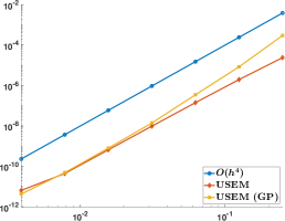
a

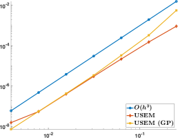
b

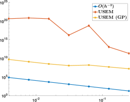
c

Figure 2: Plots of h convergence for circle interface problem with $\beta_{1}=1$ and $\beta_{2}=1000$: (a) $L^{2}$-error; (b) $H^{1}$-error; (c) Conditional number.

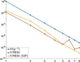
a

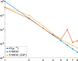
b

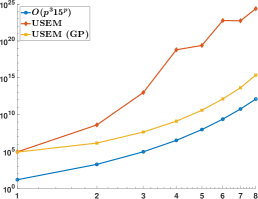
c

Figure 3: Plots of p convergence for circle interface problem with $\beta_{1}=1$ and $\beta_{2}=1000$: (a) $L^{2}$-error; (b) $H^{1}$-error; (c) Conditional number.

Firstly, we present $h$-convergence results in Figure 2 for $p=3$. As expected from our prior analysis, we observe convergence rates following:

$$O(h^{\min(p+1,m)})=O(h^{p+1})=O(h^{4}),$$

in the $L^{2}$-norm, which is consistent with our theoretical results. Similarly, a convergence rate of $O(h^{p})$ can be observed for the $H^{1}$ error. We observe that our stabilized Ghost Penalty (GP) version outperforms the standard approach in all aspects, preserving convergence rates in a superior fashion. Our graphs even suggest that this difference would become more pronounced as $h$ decreases further. Finally, we appreciate a tremendous improvement in the stiffness condition number with Ghost Penalty stabilization, with its evolution resembling $O(h^{-2})$ growth, similar to fitted Finite Element Methods.

Figure 3 presents $p$-convergence results for a grid of $16\times 16$ square elements. Regarding the $L^{2}$-error, only the Ghost Penalty (GP) version noticeably exhibits spectral convergence, initially deviating from the reference polynomial line (blue). In contrast, the non-stabilized version shows no apparent curvature, indicating a lack of spectral behavior. It’s worth noting that numerical limitations arising from double-precision arithmetic may hinder further spectral behavior beyond a polynomial degree of six. The Ghost Penalty stabilization maintains a cleaner trajectory as we approach the degree eight limit, while the standard USEM approach becomes erratic and yields somewhat unreliable results. Similar properties extend to the $H^{1}$-norm, although the overall convergence quality is notably reduced. We can only discern a hint of spectral behavior for low-order polynomial finite element bases in the GP case. Once again, a significant difference exists between the algorithms in terms of the evolution of the condition number, with even the Ghost Penalty version growing beyond an exponential rate.

5.1.2 Flower shape interface problem

In this example, we consider a flower shaped interface problem. The interface curve $\Gamma$ in polar coordinates is given by

$$r=\frac{1}{2}+\frac{\sin(5\theta)}{7},$$

which contains both convex and concave parts. The diffusion coefficient is piecewise constant with $\alpha_{-}=1$ and $\alpha_{+}=10$. The right-hand function $f$ in (3) is chosen to match the exact solution

$$u(x)=\begin{cases}e^{x_{1}^{2}+x_{2}^{2}}&\text{if }x\in\Omega^{-},\\ 0.1(x_{1}^{2}+x_{2}^{2})^{2}-0.01\ln(2\sqrt{x_{1}^{2}+x_{2}^{2}})&\text{if }x\in\Omega^{+}.\end{cases}$$

In this case, the jump conditions at the interface are nonhomogeneous and can be computed using the exact solution. The proposed unfitted spectral element method can handle interface problems with nonhomogeneous jump conditions by incorporating the corresponding terms into the right-hand side of (25), as described in [20].

a

b

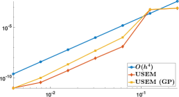
c

Figure 4: Plots of h convergence for flower shape interface problem: (a) $L^{2}$-error; (b) $H^{1}$-error; (c) Conditional number.

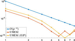
a

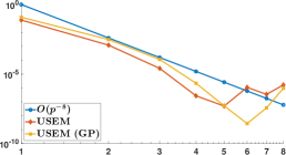
b

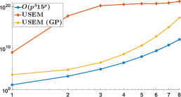
c

Figure 5: Plots of p convergence for flower shape interface problem: (a) $L^{2}$-error; (b) $H^{1}$-error; (c) Conditional number.

The $h$-convergence results presented in Figure 4 align with our theoretical expectations. In these simulations, we continued to use third-order ($p=3$) basis functions in our finite element calculations. It is evident that the $L^{2}$ convergence rate of the standard unfitted spectral element method deteriorates as we reach the last data point (the smallest $h$ value). In contrast, the Ghost Penalty (GP) version exhibits superior stability, maintaining a more consistent convergence rate. This trend is also observed in the $H^{1}$ error. As we refine the mesh, the standard unfitted spectral element method becomes increasingly susceptible to weaker numerical convergence rates, a characteristic not shared by its Ghost Penalty counterpart. In summary, the GP version consistently outperforms the standard unfitted spectral element method, and in some cases, even surpasses fitted finite element methods in terms of stiffness condition number growth. Notably, the yellow line in the right plot exhibits a less steep slope compared to the reference $O(h^{-2})$ blue line.

Given the more intricate geometry, we employed a finer grid, as compared to the previous circular test, consisting of $29\times 29$ elements. This choice allows us to better observe the desired $p$-convergence rates. In Figure 5, spectral convergence becomes quite evident. Both our unfitted spectral element method (USEM) lines, with and without Ghost Penalty (GP) stabilization, curve away from the reference polynomial rate (blue) before eventually succumbing to the limitations imposed by numerical precision. It’s important to note that the Ghost Penalty terms involve high-order derivatives, which can contribute significantly to round-off errors at higher degrees. In this case, we can observe that spectral behavior is preserved from $L^{2}$ to $H^{1}$ norms. Although our USEM curves eventually become inconsistent, the spectral tendency persists for two more degrees of $p$ with GP stabilization, thereby numerically validating its effectiveness beyond the realm of $h$-convergence. Lastly, it’s worth noting that Ghost Penalty demonstrates a remarkable improvement in the progression of the stiffness condition number. However, we also observe a growth rate that exceeds the exponential rate.

5.2 Interface eigenvalue problems

In this example, we investigate the interface eigenvalue problem (6). Our computational domain is $\Omega=(0,\pi)\times(0,\pi)$, which contains a circular interface centered at $(\frac{pi}{2},\frac{\pi}{2})$ with a radius of $\frac{\pi}{4}$, effectively splitting $\Omega$ into subdomains $\Omega_{-}$ and $\Omega_{+}$. Unlike previous cases, we now have to consider not only the stiffness matrix but also the mass matrix, adding another potential source of ill-conditioning for numerical solvers. Ghost Penalty’s contribution is thus even more significant in this scenario, as it effectively addresses instability issues stemming from both the stiffness and mass matrices. As a result, we only present the numerical results for the specific case of $\alpha_{+}/\alpha_{-}=1000$ to demonstrate the efficacy of the Ghost Penalty method.

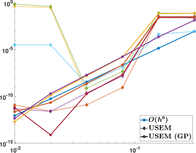
a

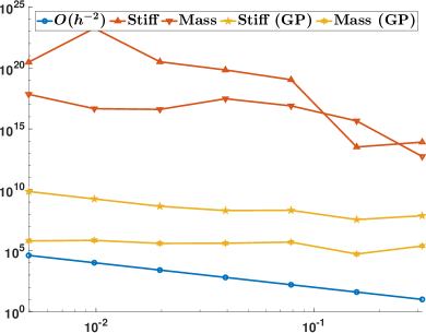
b

Figure 6: Plots of h convergence for circle interface eigenvalue problem with $\beta_{1}=1$ and $\beta_{2}=1000$: (a) eigenvalue approximation error; (b) Conditional number.

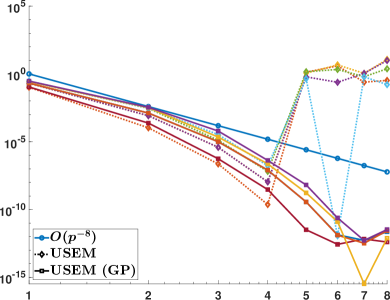
a

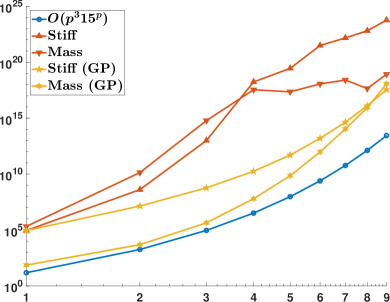
b

Figure 7: Plots of $p$-convergence for circle interface eigenvalue problem with $\beta_{1}=1$ and $\beta_{2}=1000$: (a) Eigenvalue approximation error; (b) Conditional number.

In the context of $h$-convergence (Figure 6), we set the stabilizing coefficients to $\gamma_{A}=4.1$ and $\gamma_{M}=0.002$ respectively. Aside from the initial step, we observe our expected rate of convergence,

$$O(h^{2\min(p+1,m)-1})=O(h^{2(p+1)-1})=O(h^{2p})=O(h^{6}),$$

for the USEM with Ghost Penalty Stabilization. This convergence rate aligns with our theoretical analysis and demonstrates the effectiveness of the Ghost Penalty method, which can handle problems where the solution’s regularity, $m$, exceeds the finite element functions’ degree $p$. In contrast, standard USEM struggles to maintain the theoretical convergence trajectory and becomes unstable and unreliable as we refine the mesh and reduce the mesh-to-interface intersections. Additionally, there is a noticeable difference in the progression of matrix condition numbers between the two methods. From the outset, the non-Ghost Penalty version is already in or close to the ill-conditioned range, while the Ghost Penalty matrices, both stiffness and mass, exhibit convergence rates of approximately $O(h^{-2})$ and $O(1)$ respectively, which are in line with their fitted counterparts.

For $p$-convergence in Figure 7, we set $\gamma_{A}=0.1$ and $\gamma_{M}=0.05$. In this case, both versions of USEM initially exhibit spectral convergence, with their curves deviating significantly from the reference polynomial line (blue). This behavior is notably different from the Poisson problem with the same domains $\Omega$ and $\Gamma$. However, the non-stabilized method breaks down after reaching degree $p=4$, with the error curve diverging and exhibiting random oscillations. On the other hand, GP USEM continues to descend in a spectral fashion, approaching machine precision (double arithmetic) and remaining stable even at higher degrees. Regarding the condition numbers, the main observation is that Ghost Penalty delays the inevitable and rapid increase in condition numbers, which is one of the factors contributing to the improved numerical stability of the GP algorithm. Interestingly, the stabilized mass matrix’s condition number eventually reaches and appears to overtake that of the stiffness matrix. This observation is somewhat surprising since the mass bilinear form for is much simpler than for stiffness.

6 Conclusion

In this paper, we have introduced a novel spectral element method on unfitted meshes. Our proposed method combines the spectral accuracy of spectral element methods with the geometric flexibility of unfitted Nitsche’s methods. To enhance the robustness of our approach, especially for small cut elements, we have introduced a tailored ghost penalty term with a polynomial degree of $p$. We have demonstrated the optimal $hp$ convergence properties of our proposed methods. We have conducted extensive numerical experiments to validate our theoretical results. These numerical examples not only confirm the $h$-convergence observed in existing literature but also showcase the $p$-convergence of our method.

References

- [1] C. Annavarapu, M. Hautefeuille, and J. E. Dolbow, A robust Nitsche’s formulation for interface problems, Comput. Methods Appl. Mech. Engrg., 225/228 (2012), pp. 44–54.
- [2] I. Babuška, The finite element method for elliptic equations with discontinuous coefficients, Computing (Arch. Elektron. Rechnen), 5 (1970), pp. 207–213.
- [3] I. Babuška and J. E. Osborn, Generalized finite element methods: their performance and their relation to mixed methods, SIAM J. Numer. Anal., 20 (1983), pp. 510–536.
- [4] I. Babuška and J. E. Osborn, Eigenvalue problems, in Handbook of numerical analysis, Vol. II, Handb. Numer. Anal., II, North-Holland, Amsterdam, 1991, pp. 641–787.
- [5] I. Babuška and M. Suri, The - version of the finite element method with quasi-uniform meshes, RAIRO Modél. Math. Anal. Numér., 21 (1987), pp. 199–238.
- [6] S. Badia, E. Neiva, and F. Verdugo, Linking ghost penalty and aggregated unfitted methods, Comput. Methods Appl. Mech. Engrg., 388 (2022), pp. Paper No. 114232, 23.
- [7] S. Badia, E. Neiva, and F. Verdugo, Robust high-order unfitted finite elements by interpolation-based discrete extension, Comput. Math. Appl., 127 (2022), pp. 105–126.
- [8] S. Badia, F. Verdugo, and A. F. Martín, The aggregated unfitted finite element method for elliptic problems, Comput. Methods Appl. Mech. Engrg., 336 (2018), pp. 533–553.
- [9] S. C. Brenner and L. R. Scott, The mathematical theory of finite element methods, vol. 15 of Texts in Applied Mathematics, Springer, New York, third ed., 2008.
- [10] E. Burman, Ghost penalty, C. R. Math. Acad. Sci. Paris, 348 (2010), pp. 1217–1220.
- [11] E. Burman, S. Claus, P. Hansbo, M. G. Larson, and A. Massing, CutFEM: discretizing geometry and partial differential equations, Internat. J. Numer. Methods Engrg., 104 (2015), pp. 472–501.
- [12] E. Burman and P. Hansbo, Fictitious domain finite element methods using cut elements: II. A stabilized Nitsche method, Appl. Numer. Math., 62 (2012), pp. 328–341.
- [13] Y. Cai, J. Chen, and N. Wang, A Nitsche extended finite element method for the biharmonic interface problem, Comput. Methods Appl. Mech. Engrg., 382 (2021), pp. Paper No. 113880, 24.
- [14] C. Canuto, M. Y. Hussaini, A. Quarteroni, and T. A. Zang, Spectral methods, Scientific Computation, Springer-Verlag, Berlin, 2006. Fundamentals in single domains.
- [15] Z. Chen, K. Li, and X. Xiang, An adaptive high-order unfitted finite element method for elliptic interface problems, Numer. Math., 149 (2021), pp. 507–548.
- [16] Z. Chen and J. Zou, Finite element methods and their convergence for elliptic and parabolic interface problems, Numer. Math., 79 (1998), pp. 175–202.
- [17] P. G. Ciarlet, The finite element method for elliptic problems, vol. 40 of Classics in Applied Mathematics, Society for Industrial and Applied Mathematics (SIAM), Philadelphia, PA, 2002. Reprint of the 1978 original [North-Holland, Amsterdam].
- [18] L. C. Evans, Partial differential equations, vol. 19 of Graduate Studies in Mathematics, American Mathematical Society, Providence, RI, second ed., 2010.
- [19] H. Guo and X. Yang, Gradient recovery for elliptic interface problem: I. Body-fitted mesh, Commun. Comput. Phys., 23 (2018), pp. 1488–1511.
- [20] H. Guo and X. Yang, Gradient recovery for elliptic interface problem: III. Nitsche’s method, J. Comput. Phys., 356 (2018), pp. 46–63.
- [21] H. Guo, X. Yang, and Y. Zhu, Unfitted Nitsche’s method for computing band structures of phononic crystals with periodic inclusions, Comput. Methods Appl. Mech. Engrg., 380 (2021), pp. Paper No. 113743, 17.
- [22] H. Guo, X. Yang, and Y. Zhu, Unfitted Nitsche’s method for computing wave modes in topological materials, J. Sci. Comput., 88 (2021), pp. Paper No. 24, 28.
- [23] C. Gürkan and A. Massing, A stabilized cut discontinuous Galerkin framework for elliptic boundary value and interface problems, Comput. Methods Appl. Mech. Engrg., 348 (2019), pp. 466–499.
- [24] A. Hansbo and P. Hansbo, An unfitted finite element method, based on Nitsche’s method, for elliptic interface problems, Comput. Methods Appl. Mech. Engrg., 191 (2002), pp. 5537–5552.
- [25] A. Hansbo and P. Hansbo, A finite element method for the simulation of strong and weak discontinuities in solid mechanics, Comput. Methods Appl. Mech. Engrg., 193 (2004), pp. 3523–3540.
- [26] P. Hansbo, M. G. Larson, and S. Zahedi, A cut finite element method for a Stokes interface problem, Appl. Numer. Math., 85 (2014), pp. 90–114.
- [27] S. Hou and X.-D. Liu, A numerical method for solving variable coefficient elliptic equation with interfaces, J. Comput. Phys., 202 (2005), pp. 411–445.
- [28] T. Y. Hou, X.-H. Wu, and Y. Zhang, Removing the cell resonance error in the multiscale finite element method via a Petrov-Galerkin formulation, Commun. Math. Sci., 2 (2004), pp. 185–205.
- [29] C. Lehrenfeld, High order unfitted finite element methods on level set domains using isoparametric mappings, Comput. Methods Appl. Mech. Engrg., 300 (2016), pp. 716–733.
- [30] R. J. LeVeque and Z. Li, The immersed interface method for elliptic equations with discontinuous coefficients and singular sources, SIAM J. Numer. Anal., 31 (1994), pp. 1019–1044.
- [31] Z. Li, A fast iterative algorithm for elliptic interface problems, SIAM J. Numer. Anal., 35 (1998), pp. 230–254.
- [32] Z. Li, T. Lin, and X. Wu, New Cartesian grid methods for interface problems using the finite element formulation, Numer. Math., 96 (2003), pp. 61–98.
- [33] H. Liu, L. Zhang, X. Zhang, and W. Zheng, Interface-penalty finite element methods for interface problems in , , and , Comput. Methods Appl. Mech. Engrg., 367 (2020), pp. 113137, 16.
- [34] X.-D. Liu, R. P. Fedkiw, and M. Kang, A boundary condition capturing method for Poisson’s equation on irregular domains, J. Comput. Phys., 160 (2000), pp. 151–178.
- [35] N. Moës, J. Dolbow, and T. Belytschko, A finite element method for crack growth without remeshing, Internat. J. Numer. Methods Engrg., 51 (2001), pp. 293–313.
- [36] C. S. Peskin, Numerical analysis of blood flow in the heart, J. Computational Phys., 25 (1977), pp. 220–252.
- [37] C. Ridders, A new algorithm for computing a single root of a real continuous function, IEEE Transactions on Circuits and Systems, 26 (1979), pp. 979–980.
- [38] R. I. Saye, High-order quadrature methods for implicitly defined surfaces and volumes in hyperrectangles, SIAM Journal on Scientific Computing, 37 (2015), pp. A993–A1019.
- [39] J. Shen, T. Tang, and L. Wang, Spectral methods, vol. 41 of Springer Series in Computational Mathematics, Springer, Heidelberg, 2011. Algorithms, analysis and applications.
- [40] H. Wu and Y. Xiao, An unfitted -interface penalty finite element method for elliptic interface problems, J. Comput. Math., 37 (2019), pp. 316–339.
- [41] J. Xu, Error estimates of the finite element method for the 2nd order elliptic equations with discontinuous coefficients, J. Xiangtan Univ., 1 (1982), pp. 1–5.
- [42] Z. Zhang, How many numerical eigenvalues can we trust?, J. Sci. Comput., 65 (2015), pp. 455–466.