Fourier synthesis optical diffraction tomography for kilohertz rate volumetric imaging

Abstract

Many biological processes occur at high speeds in complex 3D environments, and developing imaging techniques capable of elucidating their dynamics is an outstanding challenge. One outstanding question is understanding the interactions of active swimmers with the local physics of their viscous 3D environment. Here, we address this challenge by developing a multiplexed quantitative phase imaging approach capable of recording the 3D refractive index at kilohertz rates. Specifically, we develop Fourier synthesis optical diffraction tomography (FS-ODT), a new pattern generation and inverse computational strategy for ODT. In FS-ODT, we multiplex tens of beam angles to expand the system field of view and increase the information in single images, thereby increasing the tomogram acquisition rate. We further show that FS-ODT can simultaneously multiplex beam angles and positions to synthesize a large field of view at kilohertz framerates. We verify FS-ODT performance by imaging samples of known composition and accurately recovering the refractive index for multiplexing conditions. We then demonstrate the capabilities of FS-ODT for imaging fast diffusing microspheres in solution and single-cellular bacterial swimmers. FS-ODT is a promising approach for unlocking challenging imaging regimes that have been little explored, including measuring 3D flow fields generated by microswimmers.

Introduction

Probing biology and physics at high resolution and high speed in 3D is a tremendous experimental challenge that has inspired significant advances in imaging techniques ranging from confocal to selective-plane and structured illumination microscopy. Fluorescence microscopy is one of the most widely used techniques, but photobleaching, phototoxicity, and fluorophore photophysics limit the speed, duration, and total light dose during live cell imaging [1]. There are approaches to mitigate this problem, such as using quantum dots or monomeric fluorescent proteins. However, recent advances in quantitative phase imaging (QPI) techniques have positioned these as an alternative to fluorescence in many domains [2]. Although QPI approaches, which measure the refractive index distribution, sacrifice the molecular specificity of fluorescence, they also avoid the low-signal level, photobleaching, and fundamental tradeoffs associated with fluorescence imaging. Furthermore, the lack of fluorophores removes some of the oxidative chemical pathways believed to play an essential role in phototoxicity, with the possibility of further reducing phototoxicity by using near-infrared excitation light [3]. In many cases, when morphology and dynamics are of primary interest, QPI approaches are becoming a method of choice for long-term, high-speed volumetric imaging [4].

A variety of powerful single-shot phase imaging approaches enable fast “volumetric” imaging, including digital in-line holography [5], off-axis holography [6], and iSCAT [7]. However optical diffraction tomography (ODT) [8, 9, 10, 11, 12] has shown the most promise for rapid 3D imaging. ODT infers the 3D refractive index of a sample by combining multiple views obtained by projecting coherent light through the sample at different angles and is closely related to synthetic aperture microscopy [13] and Fourier ptychography [14]. ODT distinguishes itself in its flexibility to probe arbitrary refractive indices and non-sparse samples and obtain true volumetric images. The single-shot QPI methods, on the other hand, can only obtain unambiguous volumetric reconstructions by putting strong priors on the geometry of particles that are imaged (e.g., spheres, rods, or other particles with a known scattering model) or have inferior axial resolution [15]. Therefore, ODT stands out as the method of choice for imaging dense samples in complex environments. However, ODT imaging is typically two orders of magnitude slower than single-shot techniques due to the need to acquire $>100$ images to perform high-quality tomographic reconstruction.

Despite recent technological advances in ODT, achieving high-quality refractive index reconstructions at kilohertz volumetric imaging speeds is an open challenge. Experiments have used various techniques to generate the required illumination patterns, including galvanometric mirrors [16] and spatial light modulators (SLM’s). SLM’s are valued for their high speed and are typically placed conjugate to the sample plane where they generate tilted beams using Lee holograms [17, 18, 19], or continuous phase ramps [20]. A few approaches have alternatively placed the optics in the Fourier plane [21, 22]. Various types of SLM may be used [23, 24], but the fastest and most common choice is the digital micromirror device (DMD), a binary device often run in a grayscale mode that limits the pattern refresh rate to 1 [25, 26]. DMD’s can run at 1030 in binary mode, but this introduces stray diffraction orders that must be filtered out using static [18, 19] or dynamic [27, 28, 29] masks. Even working at the full DMD display rate, achieving high-quality ODT using $>100$ patterns limits the volumetric frame rate to ¡100, significantly slower than required for the applications discussed above. To address this, some groups have increased the frame rate by multiplexing several illumination angles into a single SLM pattern. However, due to patterning constraints, at most four angles have been combined in this way [29]. An open challenge is to further increase the volumetric imaging rate by increasing the number of simultaneous multiplexed angles.

To address this challenge, we present an alternative strategy to rationally designing and projecting ODT illumination patterns, Fourier synthesis optical diffraction tomography (FS-ODT), which is compatible with multiplexing many plane waves in a single image. FS-ODT relies on placing the DMD in the conjugate pupil plane to the objective and achieves position and angle control over the patterns using a spatial carrier frequency. Building on our previous work [30], our approach allows us to use binary DMD patterns to achieve kilohertz volumetric imaging and multiplex tens to hundreds of ODT angles in each pattern. In FS-ODT, each image contains additional information about the sample at the cost of introducing a challenging and more ill-posed reconstruction problem. To address the ill-posed problem of multiplexed patterns, we designed an iterative reconstruction approach based on multi-slice beam propagation and accelerated proximal gradient descent. In some sense, intensity diffraction tomography (IDT) inspired the FS-ODT approach presented here. IDT methods utilize LED point sources in the far-field to generate multiplex plane wave patterns and solve a joint phase retrieval and refractive index inference [31, 32]. In FS-ODT, working with coherent light and a fast pattern modulator increases flexibility by providing additional control over the beam phase and position and allows us to achieve two orders of magnitude faster volume acquisition.

In parallel with experimental advances in ODT, improving computational reconstruction techniques is a topic of great interest. As FS-ODT multiplexing introduces a more challenging computational image reconstruction problem, we briefly discuss some commonly used reconstruction approaches. In 1969, Wolf introduced optical diffraction tomography using a Born approximation formulation [8]. Devaney realized that the Rytov approximation is better suited for biological sample [9] and various technical improvements have expanded the range of validity [33, 34] and quality of reconstructions [35, 36, 37, 38, 39, 40]. However, imaging thicker and higher-contrast samples inevitably introduces multiple scattering events, which the linear Born and Rytov approximations do not include. To address multiple scattering events, a variety of multislice reconstruction approaches have been developed that rely on the beam-propagation model (BPM) [41, 42, 43, 44, 45]. However, the BPM entails the paraxial approximation, motivating the development of more accurate forward models, including the split-step non-paraxial (SSNP) model [46], more sophisticated Born approximation approaches [47, 48, 49], and HyPM [50]. Most approaches consider forward scattering only, which is implicit in the layer-by-layer multislice forward models. Other approaches account for backscattering using the Lippman-Schwinger equation [51, 52, 53, 54], but these are generally more computationally expensive than multislice models. Machine learning approaches are increasingly employed to accelerate and denoise refractive index reconstruction [55, 56]. In this work, we primarily rely on the BPM or the SSNP combined with an initial guess generated using a demultiplexed low-resolution Rytov approximation approach to infer refractive index information from FS-ODT data.

Here, we demonstrate the capabilities of FS-ODT for a variety of samples and scenarios, illustrating its unique combination of high-quality refractive index reconstruction and high-speed volumetric imaging capability. We first profile the reconstruction quality versus the degree of angle multiplexing by imaging a sample of known composition, a 10 polystyrene microsphere. Next, we consider dynamic samples, including diffusing microspheres and bacteria, and demonstrate FS-ODT tracking of colloidal particles and extraction of their hydrodynamic properties. Finally, we combine position and angle multiplexing at the fastest FS-ODT imaging rate possible with our hardware to measure diffusing microspheres at kilohertz volumetric frame rates. Taken together, the results presented here demonstrate that FS-ODT is a powerful new approach for the dynamics of cells and colloids in complex environments.

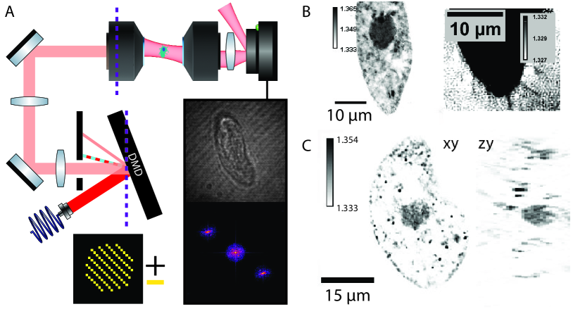
Figure 1: Fourier synthesis optical diffraction tomography. A. In FS-ODT, a spot-like pattern with a superimposed spatial carrier frequency is displayed on the DMD (lower left), which is conjugate to the back-focal plane of the objectives (purple line). The light which diffracts from the $-$ mirrors (red) at the carrier frequency is transmitted. The angle of the ODT illumination is changed by shifting the spot position, while the position of the ODT illumination is changed by shifting the carrier frequency. B. Fixed Tetrahymena imaged with FS-ODT and reconstructed in the Rytov approximation using $331$ views. Internal cell structures are resolved (left), and ∼200 cilia are at the edge of our detection ability (right). C. Fixed Tetrahymena imaged with FS-ODT and reconstructed with FISTA-BPM using $145$ views. The refractive index is shown in a single $xy$- (left) and $zy$-plane (right), and internal structure of the cell can be resolved.

Results

.1 Fourier synthesis of ODT patterns

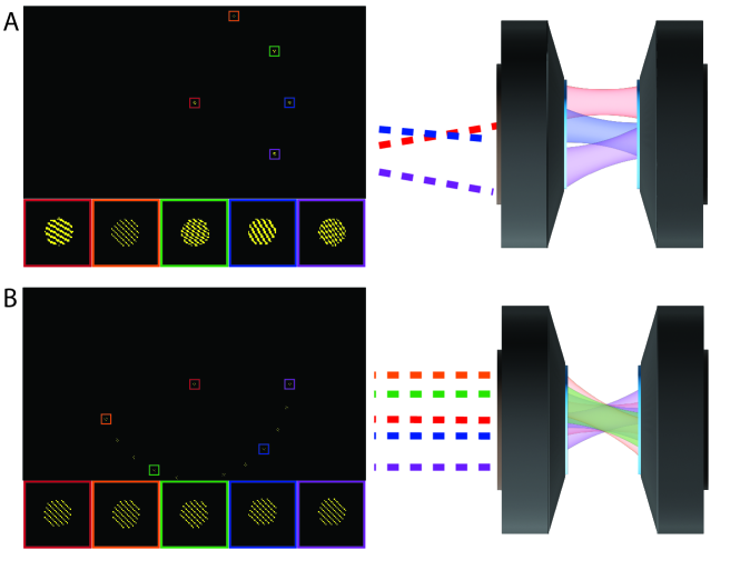
Figure 2: Multiplexed illumination with FS-ODT. A. Position multiplexing is achieved using five separate spot patterns (top left) with different carrier frequencies (inset, bottom left). When relayed to the objective back focal plane, the resulting beams have different incidence angles, and the lens transforms these angles to different positions in the focal plane. Only three beams are shown for clarity. B. Angle multiplexing is achieved using spot patterns (top left) at different spatial positions but with the same carrier frequency (inset, bottom left). When relayed to the objective back focal plane, the resulting beams have different incidence positions, and the lens transforms these positions to different angles in the focal plane.

In FS-ODT, we generate patterns using a DMD conjugate to the objective back focal (or Fourier) plane, as shown in Fig. 1A. Plane waves are encoded by circular “spot” patterns on the DMD. Varying the beam position in the sample corresponds to a adding a phase ramp in the Fourier plane, and so to make the beam position tuneable we align the system so that beams which diffract from a given spatial carrier frequency on the DMD are centered in the optical system [57]. Beam angle through the sample is encoded by spot position, so multiplexing tens to hundreds of beams at different angles is possible by displaying multiple spatially separated spot patterns on the DMD. Further, by working in the Fourier plane we avoid the need to filter stray diffraction orders as these are mitigated by Fourier broadening due to the small spot sizes. We have carefully modelled this approach by extending the DMD simulation tools we developed previously for multicolor structured illumination microscopy [30] (section S2).

To generate a single plane wave at spatial frequency $\mathbf{f}=(f_{x},f_{y})$ displaced from the center of the field of view by $\delta\mathbf{r}$, we generate a spot pattern at location $\mathbf{r}_{p}$ and spatial frequency $\mathbf{f}_{p}$ on the DMD. The object space parameters are determined by

$$\delta\mathbf{r} =\frac{f_{l}\lambda}{M}\left(\mathbf{f}_{p}-\mathbf{f}_{c}\right)$$ (1)

$$\mathbf{f} =\frac{M}{f_{l}\lambda}\left(\mathbf{r}_{p}-\mathbf{r}_{c}\right)$$ (2)

where $\mathbf{f}_{c}$ is the spatial carrier frequency, $\mathbf{r}_{c}$ is the position on the DMD aligned with the optical axis, $f_{l}$ is the focal length of the objective lens, $M$ is the magnification between the DMD and the lens back focal plane, and $\lambda$ is the wavelength of light. This approach is power inefficient as the incident beam illuminates the full DMD chip, but spot patterns of typical radius $10$ mirrors diffract only a small portion of the light. Nevertheless, since ODT detects transmitted light, there is sufficient signal to image with ¡ 100 exposure times (section A).

To validate that the proposed FS-ODT optical design is capable of high-quality 3D refractive index reconstruction, we first perform standard ODT on a complex 3D sample. We image fixed samples of the ciliate Tetrahymena using hundreds of plane waves (Fig. 1B,C). After refractive index reconstruction, we resolved the internal structure of the cell, including the nucleus, the “mouth” and the cilia, using our approach.

Next, we consider applying the FS-ODT pattern generation strategy to generate multiplexed illumination patterns. Since FS-ODT uses spatially separated spot patterns to generate plane waves at different angles, we can easily generate multiplexed patterns by displaying spot patterns at different positions on the DMD. We synthesize composite patterns from a set of beam frequencies and position shift pairs $\left\{\left(\mathbf{f}_{1},\delta\mathbf{r}_{1}\right),...\left(\mathbf{f}_{N},\delta\mathbf{r}_{N}\right)\right\}$. Each pattern consists of $N$ beams passing through the sample plane in different positions at different angles (i.e., spatial frequencies). Our approach enables two forms of multiplexing: (i) position multiplexing to extend the system field of view and (ii) angle multiplexing, which illuminates a single sample region with overlapping beams at different angles. We demonstrate these two strategies in Fig. 2. A unique benefit of FS-ODT is that these two strategies can be combined to enable angle multiplexing over a large field of view.

We use a custom Python implementation of either the BPM or the SSNP forward models  [46, 32] to reconstruct the refractive index from FS-ODT data (section S3). BPM balances quantitative reconstruction and computational cost, while SSNP provides the highest quality quantitative refractive index reconstruction. We note that although the SSNP provides results comparable to a BPM modified with the appropriate obliquity factor of the incoming plane wave [32], FS-ODT multiplexed patterns contain multiple incoming plane waves, so there is no appropriate analog of the obliquity modified BPM that can be applied here.

We solve the inverse problem using accelerated proximal gradient descent with the fast iterative shrinkage-thresholding algorithm (FISTA) [58]. FISTA and related proximal approaches have proven particularly powerful for solving ill-posed inverse image reconstruction problems because they provide a natural framework for applying regularization. Regularization stabilizes the reconstruction and favors physical solutions from all possible refractive index distributions consistent with the data. In this case, we use total variation regularization (TV), which promotes smoothness, and in some cases, $\ell_{1}$ regularization, which promotes sparsity. Additionally, we impose physical constraints, typically that the imaginary part of the refractive index is strictly absorptive (no gain) and, in certain circumstances, the real part of the refractive index is greater than the background index.

Multiplexing many patterns results in a more ill-posed inverse problem than single-beam ODT due to the additional need to unmix scattering contributions from different incident plane waves. To improve the convergence of our reconstruction algorithm, we develop an approach to initialize the refractive index with a high-quality guess in the presence of multiplexing, which we refer to as low-frequency Rytov demultiplexing. In this scheme, we rely on the presence of multiple “peaks” in the Fourier transform of the off-axis holograms, which are present if the sample is not too strongly scattering. Each peak is dominated by scattering due to a single ODT plane wave. To initialize the inverse problem, we take a small region in Fourier space around each peak and treat this as if it comes from a single plane wave. We take the resulting low-resolution demultiplexed fields and compute the Rytov phase. Finally, we use the linear scattering model to map this information to the scattering potential at the correct position in Fourier space. We found this Rytov-motivated initial guess produces a better initial guess than, e.g., beginning with a constant refractive index or mapping each position in the hologram back to multiple possible positions in the scattering potential due to the multiplexing ambiguity.

.2 10 microspheres

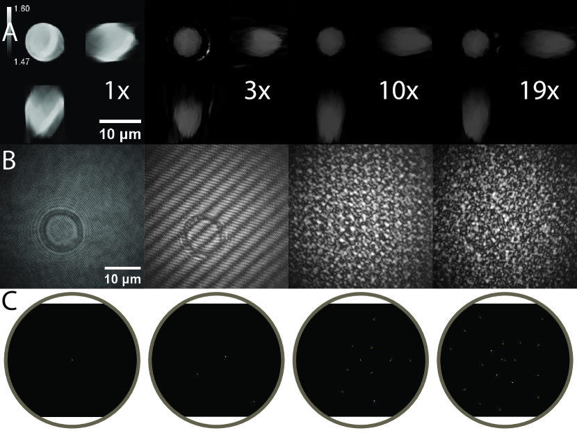
Figure 3: 10 microsphere refractice index reconstruction versus angle multiplexing. A. Refractive index reconstruction using FISTA-SSNP and an initial guess from the low-resolution demultiplexed Rytov approach described in the text. Slices through the microsphere near its center are shown in the $xy$-plane (upper left), $yz$-plane (upper right), and $xz$-plane (lower left). Results for angle multiplexing factors of $1$, $3$, $10$, and $19$ are shown (left to right) B. Exemplary raw hologram images which are used to recover the bead refractive index C. Exemplary DMD patterns used to generate the multiplexed patterns. Only the portion of the DMD within the detection objective pupil radius (grey circle) is shown. The DMD is slightly smaller (∼84) than the pupil along the vertical direction.

To assess the quality of FS-ODT reconstructions versus degree of multiplexing, we image a sample of known refractive index, a polystyrene microsphere ($n\approx$1.57$$) with diameter 10 in glycerol, $n_{o}\approx$1.47$$ (Fig. 3). We consider multiplexing by factor of $1$, $3$, $10$, $19$ using a fixed set of $N=$145$$ plane wave angles. Where the total number of angles is not divisible by the multiplexing factor, we include some plane waves twice to simplify the reconstruction. This results in a total of $145$, $49$, $15$, and $8$ raw images. We use exposure times of 600, 600, 200, and 100.

To generate the multiplexed illumination patterns, we first select $N$ plane wave angles, which approximately uniformly fill the available spatial frequency space supported by the detection objective. Due to geometric distortions introduced by the fact that our DMD is not perpendicular to the optical axis and stringent alignment requirements, we typically choose the maximum frequency to be $0.95$ of the predicted maximum frequency supported by the objective.

While FS-ODT can generate arbitrary multiplexed patterns, reconstruction quality is improved using multiplexed patterns that are easier to unmix by ensuring the beam angles in each image are as far as possible. We design our patterns using an iterative algorithm to ensure this is the case. We initialize each $M$-fold multiplexed pattern with $M$ beam angles by iteratively selecting the beam angle that maximizes the distance from those already chosen. Next, we iterate over all choices of two patterns and randomly swap beam angles. We define a loss function, the average distance between beam angles on the DMD up to a certain maximum value. If swapping the angles increases the loss function, we keep the swap. We obtain high-quality multiplexed patterns after performing $5$ iterations of $300$ swaps.

We reconstruct the microsphere refractive index using the SSNP model on a grid of size 107 x 900 x 960 with voxel sizes $dz\times dxy=\qtyproduct{0.2x0.1}{\micro}$. This array occupies ∼1.5 when stored as 128-bit complex numbers and is near the maximum we can work with on a GPU with 24 memory due to the fact our TV implementation requires $\sim 10$ times the memory of the initial array (section D). Although the reconstruction grid is significantly oversampled with respect to the Nyquist limit, it is convenient to use the camera pixel size for the $xy$ grid, and the small $z$-step is required for the SSNP to converge. Alternatively, binning the electric field by a factor of two before reconstruction can reduce the computational cost significantly. In this case we use regularization parameters $\tau_{\text{tv}}=${10}^{-3}$$ and $\tau_{\ell_{1}}=0$. Additionally we enforce the constraints that $\text{Re}(n)\geq n_{o}$ and $\text{Im}(n)=0$.

We obtain high-quality refractive index reconstructions for all multiplexing values considered in Fig. 3. With no multiplexing, we recover a nearly spherical object of the correct diameter with $n\approx 1.57$. As expected, due to the missing cone problem, the sphere appears somewhat elongated in the axial ($z$) direction. Some distortions in the bead shape may be due to the bead solution being dried on the coverslip before mounting in glycerol and imaging. As the degree of multiplexing increases, there is some underestimation of the bead’s refractive index and radius.

.3 Swimming E. coli and tracer particles

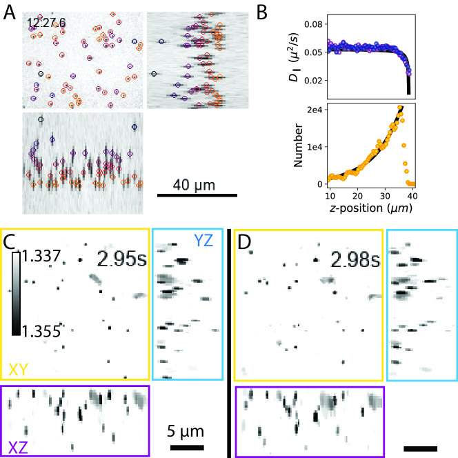
Figure 4: E. coli and tracer particles. A. 1 diameter microspheres diffusing in water-glycerol mixture imaged with FS-ODT and reconstructed with FISTA-Rytov. Maximum intensity projections of the refractive index are shown in three orthogonal planes. B. Hydrodynamic interactions between microspheres and the coverslip induce a spatially varying diffusion coefficient (top). The microspheres are buoyant in this solution, leading to a spatially varying density (bottom). C. Refractive index reconstruction of bacteria and tracer particles using FISTA-BPM max projected along three orthogonal axes, $XY$ (upper left), $YZ$ (right), and $XZ$ (bottom). The bacteria and tracers can be clearly distinguished based on their refractive index and morphology. Two bacteria (upper right) and $\sim 20$ tracer particles are visible in the $XY$ projection. D. Bacteria and tracer particles 30 later. One bacteria has rotated, and the tracers have changed position due to diffusion and advection.

Having established high-quality refractive index recovery, we now turn towards demonstrating the utility of FS-ODT to study hydrodynamics and microswimmer motility. Phase imaging approaches offer significant advantages over fluorescence imaging in lower phototoxicity, faster frame rates, and axial position sensitivity. As such, these methods are ideally suited to studying motion in 3D environments, such as the motility of colloids or cells in complex environments, which are topics of recent interest [59, 60]. 3D QPI approaches offer significant advantages over 2D-only or 2D with limited $z$ range tracking, which only measure particles at or near the microscope’s focal plane. As a first step, we demonstrate that we can image and distinguish diffusing microspheres and swimming E. coli cells in 3D using FS-ODT (Fig. 4).

Imaging dense samples introduces new reconstruction challenges, as our algorithms require knowledge of the excitation electric field with no sample present. While in some cases, the excitation field is sufficiently homogeneous such that plane wave illumination can be assumed, FS-ODT produces beams with more structure. One standard solution is to acquire a background image taken at a spatial position where no refractive index objects are present. However, for dense diffusing objects, there are no sample-free regions. Instead, we rely on the time-average image, assuming that over the long term, the refractive index inhomogeneities average out. For relatively sparse samples, this is a good approximation. For denser samples, it may be necessary to account for an average background refractive index different from the fluid medium’s. Other approaches, including joint inference of the incident electric field and the sample refractive index, are possible [61].

Before tracking microswimmers, we initially tested our dense reconstruction strategy using 1 beads diffusing in a water glycerol mixture. We performed this experiment on an early version of FS-ODT where the camera frame rate limited the maximum volumetric rate of ∼6. Nevertheless, this frame rate was sufficient to track the microspheres and measure their mean-square displacement, and hence diffusion coefficient, as a function of 3D position (Fig. 4A,B).

The diffusion coefficient is sensitive to hydrodynamic forces on the beads and serves as a sensitive indicator of hydrodynamic interactions. Colloidal particles experience hydrodynamic interactions with boundaries because they generate fluid flow fields as they move, which must satisfy the Stokes equation (in the low-Reynolds number regime) with appropriate boundary conditions. When a sphere is within a few radii, $R$, of a boundary, the no-slip boundary condition at the wall modifies the flow fields. The resulting changes affect the mobility of the sphere and, therefore, the translational and rotational diffusion coefficients. This effect is perturbative in the ratio of the distance from the wall related to the sphere’s radius $h/R$. To leading order, the effect on the diffusion coefficient parallel to the wall is [62]

$$D_{\parallel} =D_{o}\left[1-\frac{9}{16}\frac{h}{R}+\mathcal{O}\left(\frac{h^{2}}{R^{2}}\right)\right].$$ (3)

Our measured diffusion coefficients versus height above the coverslip 4B match well this functional form. There are small deviations from the expected curvature, which we attribute to the fact that the microspheres sample different heights during our measurement, leading to some broadening of the measured curve.

We also imaged swimming E. coli in solutions seeded with 0.5 microspheres as tracer particles at volumetric rates of 143 over ∼7 (Fig. 4C,D). Due to the sub-diffraction limited size of the tracer particles and bacteria, we do not expect the refractive index to be quantitative. Therefore, we multiplexed only $11$ ODT beam angles to accelerate imaging and reduce reconstruction complexity. We found that the bacteria and tracer particles can be easily distinguished based on refractive index and morphology. We observe diffusion of the tracer particles and directed swimming and rotational diffusion of the E. coli.

.4 Diffusing microspheres imaged at kilohertz volumetric rates

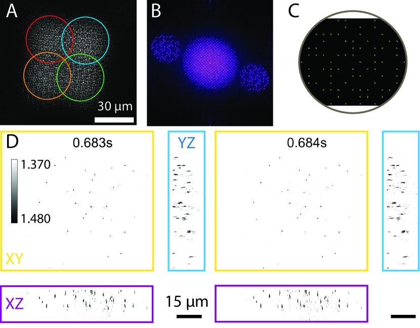
Figure 5: Diffusing microspheres at kilohertz volumetric rates with an extended field-of-view. A. Intensity profile of the beam after interacting with microspheres using $19\times$ angle multiplexing and $4\times$ position multiplexing (circles). Position multiplexing expands the usable field of view by $\sim 2\times$ B. Fourier transform of the intensity profile in A showing $76$ distinct beams in Fourier space. C. DMD pattern used to generate the illumination shown in A and B D. Refractive index reconstruction using FISTA-BPM at two time points ∼1 aparts. This time scale is faster than diffusion, so no appreciable position changes are apparent.

Finally, we demonstrate that FS-ODT leads to high-quality refractive index reconstructions running at kilohertz rates with both position and angle multiplexing. Here, we use $8$ FS-ODT patterns, each of which multiplexes $4$ positions and $19$ angles per position. This approach expands our field-of-view by a factor of $2\times$ in each lateral direction at a frame rate of 1.032. We show an exemplary angle- and position-multiplexed illumination pattern in Fig. 5A-C.

Using these highly multiplexed FS-ODT patterns, we image 1 polystyrene microspheres diffusing in water for $1000$ volumetric frames and 0.969. We reconstruct the refractive index over a volume of 20.5 x 96 x 104 x with voxel size $dz\times dxy=\qtyproduct{0.5x0.1}{\micro}$. As for other time-resolved experiments, we construct a reference electric field by averaging the images. We performed refractive index reconstruction using $100$ iterations of GPU-accelerated BPM-FISTA. Reconstruction takes ∼16, with the BPM propagation and the TV proximal operator limiting the speed. Here we used regularization strength $\tau_{tv}=$3\text{\times}{10}^{-4}$$ and $\tau_{\ell_{1}}=0$. Although we expect the SSNP model to be more accurate for these illumination patterns that include high-angle beams, the computational cost for the SSNP over this large field of view is substantial. The additional computational cost is because a finer $dz$ step is required for SSNP convergence as compared with the BPM, although the computational burden is only a factor of $\sim 2\times$ greater on an equivalent grid.

The refractive index is reconstructed separately at each time point, and exemplary time points are shown in Fig. 5D, E. Over the ∼1 interval, the beads do not move significantly. Further reconstruction improvements are possible by imposing time continuity using, for example, a Hessian proximal operator, profitably applied in other contexts [63].

Conclusion

FS-ODT is a powerful approach that extends the multiplexing capabilities of ODT, and we have demonstrated that it provides high-quality refractive index reconstructions of a variety of samples, including cells, 10 microspheres, and swimming bacteria. Multiplexing can be applied to increase the number of beam angles in a single image or expand the system field of view. Both approaches can be combined to perform fast ODT over extended lateral fields of view. We anticipate that FS-ODT will unlock challenging imaging regimes that have been difficult or impossible to explore. These include probing the ∼100 mechanical motion and hydrodynamics of cilia during swimming of protists such as Tetrahymena or exploring the behavior of microswimmers and active colloids in dense or complex 3D environments.

Despite the capabilities demonstrated here, FS-ODT can be further improved by increasing its speed and developing new computational reconstruction approaches. For example, using faster DMD models that have pattern update rates up to 30 can immediately accelerate the volumetric imaging rate by a factor of $3$. On the other hand, using FISTA or a deep learning approach to unmix the off-axis hologram, denoise raw data, suppress coherent speckle, or perform phase unwrapping will further improve the reconstruction quality. Deep learning techniques trained on paired non-multiplexed and multiplexed images might also improve the reconstructions  [55, 29]. In this case, a neural network can be thought of as incorporating a more physical regularization than ad hoc applying TV or $\ell_{1}$ regularization. Finally, in the limit of an extremely large number of multiplexed angles, FS-ODT bears some resemblance to speckle tomography [64], and it may be possible to exploit similar techniques to improve or accelerate refractive index reconstruction.

We anticipate that FS-ODT further extends the frontier of QPI to tracking and quantifying highly dynamics systems and may spur further developments in wavefront patterning and computational imaging approaches.

Data Availability

Instrument control and ODT reconstruction code is available on github [65].

Author contributions

PTB and DPS conceived the project and prepared the manuscript. PTB built the instrument, wrote the control and reconstruction code, and performed the experiments. DPS supervised all aspects of the project. RK provided assistance with sample preparation. LM and NW prepared the E. coli. EM, AP, and DFG prepared the Tetrahymena.

Supporting Information

S1 Sample Preparation

A Preparation of Tetrahymena samples

Tetrahymena were cultured at room temperature in media containing 2 proteose peptone, 0.2 yeast extract, 0.012 FeCl3, 0.2 glucose, 100/ penicillin, 100/ streptomycin, and 0.25/ Amphotericin B. Tetrahymena were passaged to fresh media every 3-4 days. Tetrahymena were stained as described previously at room temperature unless noted [66]. Briefly, $\sim 2\text{\times}{10}^{6}$ mid-log cells were washed with 10 Tris pH $7.5$, permeabilized in 0.25 TX-100 in PHEM for 30 (60 PIPES, 25 HEPES, 10 EGTA, 4 MgSO4), fixed in 1 paraformaldehyde in PHEM for 15, blocked in 3 BSA in PBS-T for 30 (0.01 Tween-20, 130 NaCl, 2 KCl, 8 Na2HPO4, 2 KH2PO4, 10 EGTA, 2 MgCl2, pH 7.5), stained with primary antibodies diluted in 3 BSA in PBS-T at 4 overnight (glutamylated tubulin 1:1000, GT335, Adipogen, AG-20B-0020-C100 and centrin 1:1000, 20H5, MilliporeSigma, 04-1624), stained with secondary antibodies diluted in 3 BSA in PBS-T for 1 hour (1:1000 goat anti-mouse IgG2a Alexa Fluor 488, Invitrogen, A-21131 and 1:1000 goat anti-mouse IgG1 Rhoadmine Red X, Jackson Immuno, 115-005-205), and counterstained with 1/ DAPI for 5 . Samples were washed with PBS three times after fixation, primary antibody incubation, and secondary antibody incubation. Each wash lasted 5 and all centrifugations were carried out for 5 at $250\times g$ in a swinging bucket centrifuge.

For the samples in Fig. 1B, we placed ∼100 of fixed Tetrahymena cells in PBS in a 40 diameter cell culture dish (FluoroDish FD5040). The single image exposure time was 1. We use $331$ plane waves arranged at the center of the pupil and $7$ annuli at 25, 45, 55, 65, 75, 84, and 95 of the pupil radius. The inner $5$ annuli include $50$ patterns arranged at equal angles. The outermost two annuli contain $46$ and $34$ patterns, respectively, as these exceed the size of the DMD along the short axis. We reconstructed the refractive index using the FISTA-Rytov approach on a grid spacing $dz\times dxy=\qtyproduct{0.869x0.202}{\micro}$ over a field-of-view of 32.2 x 47.6 x 60.9.

For the samples in Fig. 1C, 10 of fixed Tetrahymena cells in PBS were placed on a round #$1.5$ coverslip of diameter 40. A square #$1$ coverslip with 25 sides was dropped on top and the chamber was sealed with epoxy (Devcon 2 Ton Epoxy, GLU-735.90). The single-image exposure time was 0.6. We used $145$ ODT patterns with one pattern at the center of the pupil and $15$ distributed at each radius described above. We reconstructed the refractive index using the FISTA-BPM approach on grid spacings $dz\times dxy=\qtyproduct{0.87x0.2}{\micro}$ over a field-of-view of 26.97 x 50.4 x 56. The electric field data was binned by a factor of $2$ to reduce the memory required during reconstruction.

B 10 polystyrene microspheres

Polystyrene microspheres of diameter 10 (Thermofish Fluospheres F8836) were sonicated for 20 and then diluted by a factor of $100$ in EtOH. 5 were spread on a #$1.5$ coverslip of diameter 40 with a pipette tip and allowed to dry. Then 15 of glycerol was pipetted over the microspheres, and a #1 square 25x25 coverslip was dropped on top and sealed with epoxy (Devcon 2 Ton Epoxy, GLU-735.90). After the epoxy dried, the sample was placed on the microscope, and a few drops of water were placed on the top coverslip to facilitate imaging with a water dipping objective.

C Preparation of diffusing microspheres in a water-glycerol mixture

Polystyrene microspheres of diameter $2R=\qty{1}{\micro}$ (ThermoFisher Fluospheres F8823) of weight/volume 0.02 were first sonicated for 20 and then diluted by a factor of $10$ in MQ water. 10 of this dilution was combined with 40 of MQ water and 50 of glycerol. 10 of this mixture was placed on a round #$1.5$ coverslip of diameter 40. A square #$1$ coverslip with 25 sides was dropped on top, and the chamber was sealed with epoxy (Devcon 2 Ton Epoxy, GLU-735.90).

This experiment was performed on an earlier version of the apparatus. The detection objective was a $50\times$ long-working distance air objective with $\operatorname{NA}=$0.55$$ (Mitutoyu 378-805-3) and 200 focal length tube lens (Thorlabs ACT508-200-A-ML). The camera was a Prime BSI Express (Teledyne Photometrics) with 6.5 pixels and 1.8 RMS read noise. No beam expander was used after the detection tube lens. The effective pixel size was 0.130.

We used $11$ ODT patterns, including one at 0, five at 50, and five at 90 of the detection objective pupil radius arranged with equal angular separation. Due to the simple structure of the microspheres, this limited pattern set was sufficient to allow high-quality refractive index reconstruction. We acquired $10\,000$ tomograms with a single-image exposure time of 3 and a volumetric imaging rate of 6.05. The frame rate was limited by the readout time of the camera.

We reconstructed the refractive index using the Rytov approximation on a grid of $dz\times dxy=\qtyproduct{1.75x0.376}{\micro}$ over an area of $z\times y\times x=\qtyproduct{\sim 54x67x79}{\micro}$. The grid parameters were determined from the Nyquist limit based on the maximum measurable spatial frequencies given the incident beam angles and detection objective numerical aperture.

The expected refractive index of this mixture is $n_{o}=$1.407$$, the viscosity $\eta=\qty{0.0076}{}$, and the density $\rho_{\text{solvent}}=\qty{1.13}{/\milli}$ at $T=\qty{22.5}{}$. The expected diffusion coefficient far from the wall is $D_{o}=k_{B}T/6\pi\eta R=\qty{0.0579}{\micro^{2}/}$. The measured average diffusion coefficient is 0.0536^2 / . Deviations may come from differences in temperature and magnification from nominal values and the hydrodynamic interactions with the wall. The density of polystyrene is $\rho_{\text{bead}}=\qty{1.05}{/\milli}$ and therefore the microspheres are buoyant in this mixture. We observe that the height distribution of the microspheres matches a Boltzmann distribution with the expected effective mass $m=\frac{4}{3}\pi R^{3}(\rho_{\text{bead}}-\rho_{\text{solvent}})$.

After reconstructing the sample refractive index, we identified and localized the microspheres using a custom Python package, localize-psf, with GPU acceleration [67, 68, 69]. To identify candidate microspheres, we first applied a difference-of-Gaussian filter to suppress noise and background, then applied a maximum filter and selected pixels where the initial and maximum filtered images had the same values. We keep only points above a threshold. Next, we fit an ROI of size 4 x 2 x 2 around each candidate to a 3D Gaussian and only kept spots where the fit parameter was reasonable. After localizing the microspheres at all time points, we tracked them using trackpy [70, 71]. To mitigate the effect of localization errors, we computed the mean-square displacements using every $8$th frame.

D Preparation of E. coli and microspheres

A culture of Escherichia coli strain RP437, which is wild type for motility, was inoculated from a single colony and incubated overnight at 37 in Lysogeny Broth (10 tryptone, 5 yeast extract, 10 NaCl). Cultures were diluted 1:100 in T-broth (10 tryptone, 10 NaCl), and incubated at 33 while shaking at 200, until reaching an $O.D_{600}$ of $0.5$. Cells were then centrifuged at $1,200\times g$ for 7, washed, and resuspended in motility buffer (10 K2HPO4, 0.1 EDTA, pH 7.5). The mobility buffer’s refractive index was $1.333$ as measured using a refractometer (Krüss HR 901). The bacterial concentration was estimated to be 1.2e81/ using a hemacytometer (Fisher Scientific 0267151B).

Polystyrene microspheres of diameter 0.5 (ThermoFisher Fluospheres F8813) of weight/volume 0.02 were first sonicated for 20 and then diluted by a factor of $3\text{\times}{10}^{2}$ with the motility buffer and E. coli mixture. Coverslips were cleaned with EtOH. A 120 tall chamber was prepared by placing a secure seal spacer (Electron Microscopy Science Cat #70327-20S) on a round #$1.5$ coverslip of diameter 40. ∼40 of solution were placed in this chamber, and a square #$1$ coverslip with 25 sides was placed on top to close the chamber.

We acquired $1000$ tomograms with a single-image exposure time of 0.6 and a volumetric imaging rate of ∼143. We used $11$ ODT patterns with one pattern at the center of the pupil and the others arranged in an annulus at 84 of the pupil radius. We reconstructed the refractive index using the FISTA-BPM approach on grid spacings $dz\times dxy=\qtyproduct{0.435x0.196}{\micro}$ over a field-of-view of 25.6 x 25.3 x 26.5. Tracking was performed using the same workflow described for the diffusing microspheres in a water-glycerol mixture.

E Preparation of diffusing microspheres in water

Polystyrene microspheres of diameter 1 (ThermoFisher Fluospheres F8823) were sonicated for 20min and then 3 were diluted with 97 of MQ water. 10 of the dilution was pipetted on a #1.5 coverslip of diameter 40 and a square #1 coverslip with 25 sides was dropped on top. The chamber was sealed with epoxy (Devcon 2 Ton Epoxy, GLU-735.90). The height of the fluid chamber was estimated to be ∼10 from a fluorescence z-stack.

We acquired $1000$ volumes with a single-image exposure time of 75, a volumetric frame time of 0.969, and a volumetric frame rate of 1.032, limited by the maximum DMD pattern update rate. To achieve this frame rate with the camera, we cropped the chip to 960 x 1040 pixels. We used $8$ patterns, each multiplexing $19$ angles for each of $4$ positions (i.e., $76$ spot patterns on the DMD). We reconstructed the refractive index using the FISTA-BPM approach on grid spacings $dz\times dxy=\qtyproduct{0.5x0.1}{\micro}$ over a field-of-view of 20.5 x 96 x 104.

S2 Optical diffraction tomography

Optical diffraction tomography was performed using a Mach-Zender interferometer, part of a bespoke multimodal microscope with quantitative phase imaging (FS-ODT) and multicolor fluorescence superresolution microscopy (structured illumination) capabilities. Portions of this microscope are described in previous work [30]. Up to 80 of 785 light with coherence length of ∼50 is generated using a volume-holographic-grating (VHG) stabilized laser (Thorlabs FPV785P). This light is divided using a polarizing beam splitter, and the two paths are coupled into separate 1 long polarization-maintaining fibers (Thorlabs PM780-HP). One fiber is used to generate the ODT excitation light, and the other is used to generate the reference beam for the off-axis holography.

The reference beam is collimated with a molded aspheric lens of focal length 13.86 (Thorlabs C560TME-B) and beam expanded with lenses of focal length 40 (Thorlabs AC254-040-B-ML) and 300 (Thorlabs AC508-300-AB-ML). It is combined with the reference beam on a d-mirror (Thorlabs BBD1-E03) near the focal plane of the 40 lens.

The excitation light is collimated with a molded aspheric lens of focal length 18.4 (Thorlabs A280TM-B) and beam expanded by lenses with focal length 30 (Thorlabs AC254-030-AB-ML) and 125 (Thorlabs LA1986-B-ML), resulting in a Gaussian beam with waist ∼7 which is incident on the DMD.

The ODT patterns are generated from diffraction off a DMD (Texas Instruments DLP6500) with 7.56 pitch and $1920\times 1080$ mirrors. We have discussed the details of our DMD geometry elsewhere [30]. Let $\hat{\mathbf{x}}$ point along the long axes of the mirror grid and $\hat{\mathbf{y}}$ point along the short axis, both in the plane of the DMD face. Let $\hat{\mathbf{p}}=(\hat{\mathbf{x}}+\hat{\mathbf{y}})/\sqrt{2}$, $\hat{\mathbf{m}}=(\hat{\mathbf{x}}-\hat{\mathbf{y}})/\sqrt{2}$, and $\hat{\mathbf{z}}$ be the normal vector of the DMD surface pointing outwards. The DMD mirrors swivel about $\hat{\mathbf{p}}$ the axis and can be in two binary states, either $\gamma_{\pm}=\qty{\pm 12}{}$, which we will call the $+$ and $-$ states. The DMD chip is rotated so that the optical table normal points along $\hat{\mathbf{p}}$, ensuring that the principle diffraction occurs in the $mz$ plane.

The initial DMD geometry was designed to enable 3 color SIM with excitation wavelength 465, 532, and 635. For these three colors to all roughly meet the blaze condition, the DMD face normal $\hat{\mathbf{z}}$ makes an angle of $\theta_{d}\sim\qty{-21.2}{}$ with the optical axis. In the DMD coordinate system, the optical axis points along the $\sin\theta_{d}\hat{\mathbf{m}}+\cos\theta_{d}\hat{\mathbf{z}}$.

To achieve high-efficiency ODT, we align the 785 excitation light to approximately satisfy the blaze condition for the $(n_{x},n_{y})=(-3,3)$ diffraction order when the mirrors are in the $-$ state. The excitation light is incident on at an angle of approximately $\theta_{e}=\qty{6.64}{}$ so that $\hat{\mathbf{v}}_{e}=\sin\theta_{e}\mathbf{m}-\cos\theta_{e}\hat{\mathbf{z}}$. The light diffracted into $(-3,3)$ travels along the $\theta_{o}=\qty{-18.96}{}$ along $\hat{\mathbf{v}}_{o}=\sin\theta_{o}\mathbf{m}+\cos\theta_{o}\hat{\mathbf{z}}$.

As discussed in the main text, we apply an additional “carrier frequency” to our patterns of frequency $\mathbf{f}_{c}=\frac{1}{4}\hat{\mathbf{x}}-\frac{1}{4}\hat{\mathbf{y}}\ 1/\text{mirror}$. This produces additional diffraction about the $(-3,3)$, and we have designed our system such that the $(-3,3)+(1/4,-1/4)$ diffraction order travels along the optical axis and is nearly blazed. The perfectly blazed output direction for the $-$ mirrors is $\sin\theta_{b}\hat{\mathbf{p}}+\cos\theta_{b}\hat{\mathbf{z}}$ for $\theta_{b}=\qty{-17.36}{}$. An aperture blocks all other diffraction orders. This specific carrier frequency is chosen to displace the beam as far as possible from orders of the form $(n/2,m/2)$, as we see significant diffraction due to the $+$ mirror states. Furthermore, this avoids diffraction along the $\hat{\mathbf{x}}$ and $\hat{\mathbf{y}}$ axes coming from a row of DMD mirrors beyond the active chip, which are fixed in the $-$ state.

The DMD is in a conjugate plane to the back focal plane (Fourier plane) of the excitation and detection objectives. After light diffracts off of the DMD, it is relayed by a pair of imaging systems, the first using lenses of focal length 200 (Nikon MXA20696) and 100 (Thorlabs AC508-100-A-ML), and the second using lenses of 400 (Thorlabs AC508-400-A-ML) and 300 (Thorlabs AC508-300-A-ML). After the Nikon tube lens, the NIR light is separated from the visible light with a dichroic mirror (Semrock FF750-SDi02-25x36). After the 100 achromat, they are recombined using a second identical dichroic mirror. The two dichroic mirrors are arranged at right angles to each other to avoid the differential $s$– and $p$–phase shifts from affecting the polarization of the visible light [72]. We align the polarization orthogonal to the table surface to avoid similar polarization degradation of the ODT beam by the epifluorescence dichroic for the fluorescence modality.

The ODT light is focused with an oil immersion objective (Olympus UPlanFL N 100x NA 1.3), interacts with the sample, and is collected using a water objective (Olympus LUMPLFLN60XW) and a 180 tube lens (Thorlabs AC508-180-AB-ML). The image is then magnified by a factor of $3$ using a relay composed of a 100 (Thorlabs AC508-100-B-ML) and 300 (Thorlabs AC508-300-AB-ML) lenses. The light is imaged onto a Phantom camera (VEO-1010L-72G-M) which has 1280 x 960 pixels, pixel size 18, quantum efficiency ∼51 at 785, read-noise 10.5 RMS and gain of 0.39/ , measured using the approach of [73]. The effective pixel size is 0.1. The maximum frame rate for the full chip is 8420

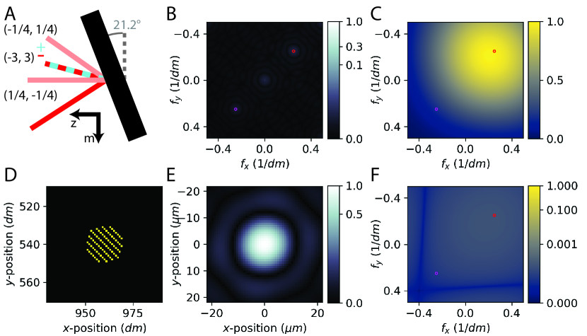
Figure S1: DMD geometry and pattern simulation. A. DMD geometry showing the incident NIR light (red) and the main diffraction orders for the $+$ (cyan) and $-$ (red) mirrors and the positive and negative diffraction at the carrier frequencies (pale red) B. Magnitude squared of the diffracted electric field versus frequency, $|E(f)|^{2}$. The diffracted weight is concentrated around the positive (red) and negative (magenta) carrier frequency diffraction orders C. Blaze envelope for $-$ mirrors. D. Sample DMD pattern with $R=\qty{10}{}$ show mirrors in the $-$ state (red) and the $+$ state (cyan) E. Pattern in sample plane with measured waist $w_{o}=\qty{9.3}{\micro}$ F. Blaze envelope for the $+$ mirrors. The strength of this diffraction is suppressed by $\sim{10}^{-5}$ compared with the $-$ mirrors.

A DMD efficiency

The expected peak DMD diffraction efficiency into any order $(n_{x},n_{y})$ is ∼50, limited by the reflective of the DMD mirrors, the fraction of the chip the mirrors cover, the transmissivity of the DMD window, and diffraction physics. Using the carrier frequency, we expect that efficiency into the $\pm 1$ carrier orders are each ∼25 of the power in the $0$th order. We expect the power in $0$th order is ∼18 of the power that would be diffracted if the mirrors were all in the $-$ state. Taken together, we estimate the DMD diffraction efficiency into the desired order is ∼2.

The fiber coupling efficiency is ∼50. Additionally, since the fluorescence modality of our microscope operates at visible wavelengths, most of the optical coatings are optimized for visible light. Thus, only ∼75 of light diffracted from the DMD reaches the objectives. The two objective lenses have a combined transmissivity of ∼50. The efficiency from the DMD to the camera is thus ∼30,

As only a small fraction of the DMD mirrors are used to generate a plane wave, this further reduces the efficiency. We adjust the magnification between the back focal plane and the DMD so that the pupil radius is approximately the same size as the DMD along its narrow dimension. As the magnification factor is $M=$0.625$$, the detection objective pupil radius is $R_{p}=\operatorname{NA}f/0.625=\qty{4.8}{\milli}$ at the DMD. For a spot pattern of radius $R$ and assuming the laser power is distributed uniformly over the pupil, we expect the number of photons per second that strike the camera is

$$\frac{\qty{80}{\milli}}{hc/\lambda}\times\frac{\pi R^{2}}{\pi R^{2}_{p}}\times\left(0.5\times 0.02\times 0.3\right)\approx\qty{2e11}{/}.$$ (S1)

for $R=10\times\qty{7.56}{\micro}$. Here, we divide the terms into incident power, geometric efficiency, and transmission/diffraction efficiency.

For patterns of radius $10$ mirrors, our simulations show that the beam waist in the imaging plane is ∼10 (Fig. S1E), and putting this all together, for an imaging time of 100 we expect to collect about

$$N=\qty{2e11}{/}\times\frac{\left(\qty{20}{\micro}\times\frac{1}{180}\right)^{2}}{\pi\left(\qty{10}{\micro}\right)^{2}}\times\qty{100}{\micro}\times\operatorname{QE}\sim\qty{400}{}$$ (S2)

per pixel, where the quantum efficiency of the camera is $\operatorname{QE}\sim\qty{50}{}$ at 785.

B Pattern fidelity

Previous ODT approaches using binary DMD patterns have resulted in lower-quality reconstruction than gray-scale approaches due to the unwanted additional diffraction orders introduced by the DMD’s square binary pixels. Our previous structured illumination microscopy work addressed similar issues [30]. In both cases, these spurious diffraction orders arise when using large-scale periodic patterns covering the face of the DMD. In this case, our small spot patterns lead to much smaller contributions from these orders, which are mitigated by Fourier broadening (Fig. S1B).

C DMD non-planarity

Unlike in many DMD imaging applications, we do not place the DMD orthogonal to the optical axis (Fig. S1A). This compromise improves the diffraction efficiency by satisfying the blaze condition. In our geometry, the effect of this tilt is minor.

The tilt introduces a shift in the focus of the plane waves across the DMD face. At the pupil radius, the DMD $z$-shift is at most $R_{p}\sin\theta_{D}\sim\qty{1.73}{\milli}$. As the $z$-magnification is $M_{z}=M^{2}=$0.39$$ the shift in the objective back-focal plane is 0.67. The shift must be compared with the depth-of-focus of the beam in the back focal plane, which we estimate using the Rayleigh range. For a plane wave with $w_{o}=\qty{10}{\micro}$ in the focal plane, the waist in the objective BFP is ∼37 corresponding to a Rayleigh range of $\pi w_{o}^{2}/\lambda\sim\qty{5.5}{\milli}$, which is one order of magnitude larger than the focal shift.

The tilt also introduces deformations in the transformation between the position on the DMD face and the frequency of the beam. For example, there is some shear, and a ring pattern on the DMD maps to an oval in frequency space. The precise effects can be calculated using the approach of [30] described in section 3 of the supplemental methods.

D Computer control and refractive index reconstruction

The microscope is controlled using a custom computer package and a GUI based on Napari-MicroManager, which relies on the MicroManager device drivers but replaces the Java GUI with Napari. The DMD and Phantom camera are controlled using custom Python code. The ODT patterns are pre-loaded on the DMD firmware, and the entire microscope acquisition is hardware triggered by a National Instruments DAQ (PCIe-6343).

We implemented light scattering forward models and proximal gradient algorithms in Python, harnessing CuPy for GPU acceleration and Dask for parallelization and orchestration [65]. We rely on the RAPIDS cuCIM implementation of the total variation proximal operator, which is modeled on the scikit-image implementation, denoise_tv_chambolle.

We use a Lenovo ThinkStation P620 running Microsoft Windows 10 Enterprise for reconstruction and experimental control. This computer has an AMD Ryzen Threadripper Pro 3945WX CPU with $12$ cores, 128 RAM, and an NVidia GeForce RTX 3090 (Ampere) GPU with 24 memory. We run CUDA 11.8 and Python 3.11. The Phantom camera includes 72 on-board memory and the 10 Gigabit ethernet option. It communicates with the PC using an X540-T2 10GbE card. A full 72 camera acquisition can be transferred to the computer in ∼2.

E System stability

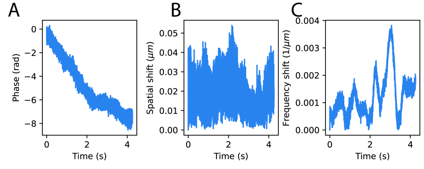
Figure S2: System stability. A. Exemplary phase stability plot from the first pattern from the 10 bead data. Phases are unwrapped B. Exemplary pattern position stability for the same pattern as A. C. Exemplary pattern frequency stability for one frequency in the pattern in A.

Due to the relatively long beam path ($>\qty{2}{}$) used in our multimodal microscope setup, we observe several sources of instability in our system and ODT patterns, which we correct for computationally during ODT reconstruction. Specifically, we correct for (1) phase drift between the reference arm and the imaging arm, (2) frequency instability of the ODT patterns, and (3) position instability of the ODT patterns.

To correct for (1), we determine the complex factor relating the image electric fields to a single background electric field using a least-squares fit. To correct for (2), we determine the location of the Fourier peaks versus time by fitting the Fourier transform of the hologram image to a Gaussian in the vicinity of each peak. To correct for (3), we register images using the Fourier transform of the absolute value of the electric field. Empirically, we find that using the absolute value of the electric field is superior to using either the Fourier transform of the intensity or the Fourier transform of the electric field. The improvement is likely due to the rejection of background fluctuations that do not involve the interference pattern and taking the absolute value removes the need to consider phase fluctuations of the electric field.

The stability of our system over ∼4 is shown in Fig. S2. Over this short time span the relative phase between the imaging and reference beam drifts by $\sim 2\pi$ radians, the spatial position drifts by ¡ 50, and the beam frequency drifts by ¡ 4e-3^-1. Note that the Fourier space pixel sizes are $df_{x}=\qty{7.81e-3}{\micro^{-1}}$ and $df_{y}=\qty{10.42e-3}{\micro^{-1}}$, so the frequency drift is sub-pixel.

S3 Iterative reconstruction with proximal gradient methods

We treat refractive index reconstruction as a regularized minimization problem and solve it using the fast iterative shrinkage-thresholding algorithm (FISTA) [58]. As usual in FISTA, we attempt to minimize a function which is the sum of two terms, a loss function and a regularization function $\mathcal{L}(x)+g(x)$, where $\mathcal{L}$ is differentiable and has a Lipschitz-continuous gradient with Lipschitz constant $L$ and $g$ is convex. We iterate starting from $t=0$, $q_{0}=1$, the step-size $\gamma$, and an initial object $x_{o}$

$$y_{t} =\operatorname{prox}_{\gamma_{t}}\left[x_{t-1}-\gamma\nabla\mathcal{L}(x_{t-1})\right]$$

$$q_{t} =\frac{1+\sqrt{1+4q_{t-1}^{2}}}{2}$$

$$x_{t+1} =y_{t}+\frac{q_{t-1}-1}{q_{t}}\left(y_{t}-y_{t-1}\right).$$

In the last step the convergence is accelerated by including a momentum term and the structure of $q_{t}$ is chosen to change the convergence from $\mathcal{O}(1/t)$ to $\mathcal{O}(1/t^{2})$.

The proximal operator for $g$,

$$\operatorname{prox}_{\gamma}(z)=\operatorname{argmin}_{x}\left\{g(x)+\frac{1}{2\gamma}\left|x-z\right|^{2}\right\},$$ (S3)

determines a new object which is near to the initial value but better satisfies the regularization. When an explicit form of or fast algorithm for computing the proximal operator is known, this process is efficient, as in the case of total variation [74], $\ell_{1}$, or $\ell_{2}$ norms. In this work we choose a regularization function which enforces smoothness and sparsity

$$g(x)=\tau_{\text{tv}}TV(x)+\tau_{\ell_{1}}\lVert x\rVert_{1}.$$ (S4)

The total loss, $\mathcal{L}(x_{t})+g(x_{t})$, is non-increasing when the step-size $\gamma\in[0,2/L]$. If the Lipschitz constant is not known, a line-search strategy can determine the step-size at each iteration by reducing an initial step-size until the Lipschitz condition is locally satisfied (algorithm 1). This requires additional calculation of $\mathcal{L}(y)$, $\mathcal{L}(x)$, and $\nabla\mathcal{L}(y)$.

Data: Proposed object $x$

Data: Initial step-size $\gamma_{o}$

Data: Step-size adjuster $f<1$

$\gamma\leftarrow\gamma_{o}$;

$y\leftarrow\operatorname{prox}\left[x-\gamma\nabla\mathcal{L}(x)\right]$;

while $\mathcal{L}(y)>\mathcal{L}(x)+\nabla\mathcal{L}(x)\cdot(y-x)+\frac{1}{2\gamma}\lVert y-x\rVert^{2}_{2}$ do

       $\gamma\leftarrow f\gamma$;

       $y\leftarrow\operatorname{prox}\left[x-\gamma\nabla\mathcal{L}(x)\right]$;

      

end while

Algorithm 1 Line-search algorithm for setting the step-size

In ODT, we measure a sequence of electric fields $\mathbf{\Psi}^{(i,d)}$, where $i=1,...,M$ indexes the incident angles, derived from off-axis holography and define our loss function by

$$\mathcal{L}(n) =\frac{1}{2NM}\sum_{i=1}^{M}\left(\mathbf{\Psi}^{(i)}-\mathbf{\Psi}^{(i,d)}\right)^{\dagger}\left(\mathbf{\Psi}^{(i)}-\mathbf{\Psi}^{(i,d)}\right)$$ (S5)

where $\mathbf{\Psi}^{(i)}(n)$ is the forward model describing the predicted electric field as a function of $n$ and $N$ is the number of pixels in a single electric field.

We take the derivative of the loss function with respect to the refractive index, which only acts directly on the forward model. Suppose $b$ and $l$ index the $xy$- and $z$-position of the voxels respectively, then we have (suppressing the beam angle index)

$$\frac{\partial\mathcal{L}}{\partial n^{\prime}_{b}(z_{l})} =\frac{1}{2}\frac{\partial\mathbf{\Psi}^{\dagger}}{\partial n^{\prime}_{b}(z_{l})}\mathbf{D}+\text{c.c.}=\frac{1}{2}\sum_{a}\left(\frac{\partial\Psi_{a}}{\partial n^{\prime}_{b}(z_{l})}\right)^{*}D_{a}+\text{c.c.}$$ (S6)

$$\nabla_{n}\mathcal{L} =\nabla_{n^{\prime}}\mathcal{L}+i\nabla_{n^{\prime\prime}}\mathcal{L}$$ (S7)

where $n^{\prime}$ is the real part of the refractive index and $\mathbf{D}^{(i)}=\mathbf{\Psi}^{(i)}-\mathbf{\Psi}^{(i,d)}$ is the difference vector between the forward model and the data. The derivative with respect to the imaginary part of the refractive index, $n^{\prime\prime}$, is similar.

A Linear scattering models

As usual we suppose light interacts with a spatially varying refractive index according to the scalar Helmholtz equation and work with phasors carrying $\exp(i\omega t)$ time dependence,

$$\left[\nabla^{2}+k^{2}n^{2}(\mathbf{r})\right]E(\mathbf{r}) =0.$$ (S8)

where $k=2\pi/\lambda n_{o}$.

Additionally we define the scattering potential $V$

$$V(\mathbf{r}) =-\left(\frac{2\pi}{\lambda}\right)^{2}\left[n^{2}(\mathbf{r})-n_{o}^{2}\right]$$ (S9)

We suppose that our sample is illuminated by a sequence of plane waves and the $i$th plane wave has frequency $\mathbf{f}^{(i)}$

$$E^{(i,o)} =\exp\left[-i2\pi\mathbf{f}^{(i)}\cdot\mathbf{r}\right]$$ (S10)

where $2\pi\left\lvert\mathbf{f}^{(i)}\right\rvert=k$.

In the Born approximation, valid when the cumulative phase shift of the beam is $\lesssim\pi/4$ [75], the 2D Fourier transform of the scattered electric field gives the scattering potential along a spherical cap in 3D Fourier space

$$\tilde{E}^{(i,s)}(f_{x},f_{y}) =\frac{1}{2i\times 2\pi f_{z}(f_{x},f_{y})}\tilde{V}(f_{x}-f^{(i)}_{x},f_{y}-f^{(i)}_{y},f_{z}-f^{(i)}_{z})\;\text{(Born)}$$ (S11)

The Rytov approximation is an alternate approach which is usually more accurate for biological samples. In this approximation, the scattering potential is related to the Rytov phase $\psi(\mathbf{r})$,

$$E^{(i,s)}(\mathbf{r}) =E_{o}(\mathbf{r})\left(e^{\psi^{(i)}(\mathbf{r})}-1\right)$$ (S12)

$$\psi^{(i)}(\mathbf{r}) =\log\left|\frac{E^{(i)}(\mathbf{r})}{E^{(i,bg)}(\mathbf{r})}\right|+i\ \text{unwrap}\left\{\text{angle}\left[E^{(i)}(\mathbf{r})\right]-\text{angle}\left[E^{(i,bg)}(\mathbf{r})\right]\right\}$$ (S13)

$$\tilde{\psi}^{(i)}(f_{x}-f_{x}^{(i)},f_{y}-f_{y}^{(i)}) =\frac{1}{2i\times 2\pi f_{z}(f_{x},f_{y})}\tilde{V}(f_{x}-f_{x}^{(i)},f_{y}-f_{y}^{(i)},f_{z}-f_{z}^{(i)})\;\text{(Rytov)}$$ (S14)

The Rytov approximation is valid when $n^{2}(\mathbf{r})-n_{o}^{2}\gg\left\lvert\nabla\psi(\mathbf{r})\right\rvert^{2}k^{2}$ [9].

In this case, it is more convenient to work with the scattering potential than the refractive index, and the loss function (eq. S5) and its gradient are

$$\mathcal{L}(V) =\frac{1}{N}\frac{1}{2MN}\sum_{i=1}^{M}\sum_{j=1}^{N}\left|\left(F^{(i)}\tilde{V}\right)_{j}-\tilde{\Psi}^{(i)}_{j}\right|^{2}$$

$$\nabla_{\tilde{V}}\mathcal{L} =\frac{1}{N}\frac{1}{MN}\sum_{i}\left(F^{(i)}\right)^{\dagger}\left(F^{(i)}\tilde{V}-\tilde{\mathbf{\Psi}}^{(i)}\right)$$

where $\tilde{\mathbf{\Psi}}^{(i)}$ is the scattered field or the Rytov phase depending on the approximation, $F^{(i)}$ is the forward model linear operator for the $i$th angle which connects the 3D Fourier transform of the scattering potential, $\tilde{V}$, to $\tilde{\mathbf{\Psi}}^{(i)}$. The second factor of $1/N$ converts this to the per-pixel loss in real-space accounting for the Fourier transform. Since the forward model is linear, a Lipschitz constant for the loss function is proportional to the largest eigenvalue of $F^{t}F$ which can be computed using a singular value decomposition or the power iteration algorithm.

B Phase unwrapping

Applying the Rytov approximation to obtain an initial refractive index distribution requires a phase unwrapping step (eq. S13). This is critical to the reconstruction performance because it must initialize the solver in the correct local minimum. Consider the case of a sphere of homogeneous refractive index and a straight-on incident plane wave. Near the center of the sphere, the beam experiences a phase shift of $\Delta\phi$, which is measured modulo $2\pi$. The number of phase wraps can be determined from the way the phase interpolates between $\Delta\phi$ and $0$ at the edge of the beam, beyond the region where the light interacts with the sphere. When phase unwrapping fails, $\Delta\phi$ is predicted with the wrong multiply of $2\pi$. The solver cannot escape by increasing the refractive index enough to induce an extra phase wrap because in between the predicted $\Delta\phi$ is wrong, leading to increased loss function.

Due to the spatial structure of the multiplexed patterns, there are regions where interference leads to zero amplitude for the electric field. These zeros cause phase unwrapping methods which require a path in 2D to be brittle. Instead, we apply a method based on mapping the phase unwrapping to a Poisson equation with Neumann boundary conditions which can be solved using the discrete cosine transform [76]. This method can be modified to handle the weighted phase unwrapping problem, although this requires an iterative procedure resulting in a slower algorithm. However, we find using the electric field magnitude as the weight parameter results in more robust phase unwrapping.

C Multi-slice models

Suppose that we can rewrite the Helmholtz equation (eq. S8) by reparameterizing the electric field as $\Psi$ and rewriting the differential operator as the sum of two terms, where $A$ describes the effect of the background refractive index $n_{o}$ and $B$ captures the effect of spatially varying refractive index perturbations,

$$\partial_{z}\Psi =\left(A+B\right)\Psi.$$ (S15)

Formally the solution is a path-ordered exponential, but for small enough $\delta z$,

$$\Psi(\delta z) \approx\exp\left[(A+B)\delta z\right]\Psi(0)$$ (S16)

$$\approx\exp\left[A\delta z\right]\exp\left[B\delta z\right]\Psi(0).$$ (S17)

For convenience we define $P=\exp\left[A\delta z\right]$ and $Q=\exp\left[B\delta z\right]$. Corrections to eq. S17 are given by the Baker-Campbell-Hausdorff formula, and the first correction is proportional to the commutator $[A,B]$. By construction, this vanishes when $n=n_{o}$, and we expect it and higher order commutators to be small when the refractive index perturbation is small.

We can propagate an initial field through a volume by discretizing it into layers of thickness $\delta z$ and iteratively applying eq. S17

$$\Psi =F(PQ)^{(k-1)}...(PQ)^{(0)}\Psi^{(0)}$$ (S18)

Here $F$ describes model operations beyond the final refractive index plane, $\Psi^{(m)}$ is the intermediate field before the $m$th voxel, and $\Psi$ is the detected field.

For models considered here, $Q$ is local in the sense that the only dependence on $n(z=z_{l})$ is in $Q^{(l)}$, and thus

$$\frac{\partial\Psi_{a}}{\partial n^{\prime}_{b}(z_{l})} =\sum_{cd}W^{(l+1)}_{ac}\frac{\partial Q^{(l)}_{cd}}{\partial n^{\prime}_{b}(z_{l})}\Psi^{(l)}_{d}$$ (S19)

$$W^{(l+1)} =F(PQ)^{(k-1)}...(PQ)^{(l+1)}P^{(l)}.$$ (S20)

Typically the structure of $\partial Q$ allow us to simplify this expression. For example, in the BPM $Q$ is diagonal due to the fact it does not mix the field at different $\mathbf{r}$ positions. For the SSNP, $Q$ is local but mixes the derivative and field at the same position.

D Beam-propagation model (BPM)

In the BPM, the Helmholtz equation is put in the form of eq. S15 by first making the paraxial approximation [43]. Here we take $\Psi=E$ and the model is defined by

$$P\Psi =\mathcal{F}_{\perp}^{-1}\left\{e^{i\delta z\sqrt{k^{2}-k_{x}^{2}-k_{y}^{2}}}\times\mathcal{F}_{\perp}\left\{\Psi\right\}(k_{x},k_{y})\right\}$$ (S21)

$$Q\Psi =\exp\left[ik_{o}\delta z\left(n(x,y,z_{o})-n_{o}\right)\right]\times\Psi$$ (S22)

$$F\Psi =\mathcal{F}_{\perp}^{-1}\left\{H(k_{x},k_{y})\times e^{i\delta z_{f}\sqrt{k^{2}-k_{x}^{2}-k_{y}^{2}}}\times\mathcal{F}_{\perp}\left\{\Psi\right\}(k_{x},k_{y})\right\}$$ (S23)

where $H$ is the coherent transfer function, $\delta z_{f}$ is the final distance the beam propagates, and $k_{o}=2\pi/\lambda$.

Following eqs. S6 and S19 the derivatives are

$$\frac{\partial Q^{(l)}_{cd}}{\partial n^{\prime}_{b}(z_{l})} =ik_{o}\delta z\ \exp\left[ik_{o}\delta z(n_{c}(z_{l})-n_{o})\right]\times\delta_{cd}\times\delta_{bd}$$ (S24)

$$\frac{\partial\Psi_{a}}{\partial n^{\prime}_{b}(z_{l})} =ik_{o}\delta z\left(F(PQ)^{(k-1)}...(PQ)^{(l+1)}\right)_{ab}\Psi^{(l+1)}_{b}$$ (S25)

$$\frac{\partial\mathcal{L}}{\partial n^{\prime}_{b}(z_{l})} =-\frac{ik_{o}\delta z}{2N}\sum_{a}\left(F(PQ)^{(k-1)}...(PQ)^{(l+1)}\right)_{ab}^{*}D_{a}\left(E^{(l+1)}_{b}\right)^{*}+\text{c.c.}$$ (S26)

$$\nabla_{n(z_{l})}\mathcal{L} =-ik_{o}\delta z\frac{1}{N}\left[\left(F(PQ)^{(k-1)}...(PQ)^{(l+1)}\right)^{\dagger}\mathbf{D}\right]\odot\left(\Psi^{(l+1)}\right)^{*}.$$ (S27)

E Split-step non-paraxial model (SSNP)

This model is extensively discussed elsewhere [46, 32] and we briefly discuss it here for convenience. To rewrite the Helmholtz equation in the form of eq. S15 we must work with a vector of the electric field and its first derivative. The physical intuition behind this is as follows. Suppose we know the electric field in a single plane and wish to know its value everywhere. We can decompose the field into Fourier modes, but we cannot distinguish forward and backwards travelling plane waves at the same lateral spatial frequency. We need additional information to untangle these two contributions: e.g. the magnetic field or the axial derivative of the electric field $\partial_{z}E$. Therefore the propagation operator must act on both the field and its derivative.

In this case the forward model is

$$\Psi =\begin{pmatrix}E\\ \partial_{z}E\end{pmatrix}$$ (S28)

$$P\Psi =\mathcal{F}_{\perp}^{-1}\left\{\begin{pmatrix}\cos k_{z}\delta z&\frac{1}{k_{z}}\sin k_{z}\delta z\\ -k_{z}\sin k_{z}\delta_{z}&\cos k_{z}\delta_{z}\end{pmatrix}\mathcal{F}_{\perp}\left\{\Psi\right\}\right\}$$ (S29)

$$Q\Psi =\begin{pmatrix}1&0\\ k_{o}^{2}(n_{o}^{2}-n^{2})\delta z&1\end{pmatrix}\Psi$$ (S30)

$$F\Psi =\mathcal{F}_{\perp}^{-1}\left\{\begin{pmatrix}\frac{1}{2}&\frac{1}{2}\frac{1}{ik_{z}}\end{pmatrix}H(k_{x},k_{y})\times P(\delta z_{f})\Psi\right\}.$$ (S31)

When we write $Q$ as a matrix following eq. S19 we combine the structure of the $\mathbf{r}_{\perp}$ index and the field/derivative index. Let $i$ and $j$ index the position $\mathbf{r}_{\perp}$ and field/derivative respectively and define the composite index $c=2i+j$. Following eqs. S6, S19, and S20, the derivatives are

$$\frac{\partial Q_{cd}}{\partial n^{\prime}_{b}} =-2k_{o}^{2}\ \delta z\ n\times\delta_{c,2b+1}\ \delta_{d,2b}$$ (S32)

$$\frac{\partial E_{a}}{\partial n^{\prime}_{b}(z_{l})} =-2k_{o}^{2}\ \delta z\ n_{b}\times W^{(l+1)}_{a,2b+1}\Psi_{2b}^{(l)}$$ (S33)

$$\frac{\partial\mathcal{L}}{\partial n^{\prime}_{b}(z_{l})} =-k_{o}^{2}\ \delta z\sum_{a}\left(W_{a,2b+1}^{(l+1)}\right)^{*}D_{a}\left(\Psi_{2b}^{(l)}\right)^{*}n_{b}^{*}(z_{l})+\text{c.c.}$$ (S34)

$$\nabla_{n}\mathcal{L} =-2k_{o}^{2}\ \delta z\left[\left(\hat{W}^{(l+1)}\right)^{\dagger}\mathbf{D}\right]\odot n^{*}(z_{l})\odot\left(\mathbf{E}^{(l)}\right)^{*}.$$ (S35)

where in the last line we use $\Psi_{2b}=E_{b}$ and define $\hat{W}$, a modified version of $W$ which retains only the derivative parts of the second index.

References

- Laissue et al. [2017] P. P. Laissue, R. A. Alghamdi, P. Tomancak, E. G. Reynaud, and H. Shroff, Assessing phototoxicity in live fluorescence imaging, Nature Methods 14, 657 (2017).
- Javidi et al. [2021] B. Javidi, A. Carnicer, A. Anand, G. Barbastathis, W. Chen, P. Ferraro, J. W. Goodman, R. Horisaki, K. Khare, M. Kujawinska, R. A. Leitgeb, P. Marquet, T. Nomura, A. Ozcan, Y. Park, G. Pedrini, P. Picart, J. Rosen, G. Saavedra, N. T. Shaked, A. Stern, E. Tajahuerce, L. Tian, G. Wetzstein, and M. Yamaguchi, Roadmap on digital holography, Optics Express 29, 35078 (2021).
- Chen et al. [2020a] G. Chen, Y. Cao, Y. Tang, X. Yang, Y. Liu, D. Huang, Y. Zhang, C. Li, and Q. Wang, Advanced Near-Infrared Light for Monitoring and Modulating the Spatiotemporal Dynamics of Cell Functions in Living Systems, Advanced Science 7, 1903783 (2020a).
- Park et al. [2018] Y. Park, C. Depeursinge, and G. Popescu, Quantitative phase imaging in biomedicine, Nature Photonics 12, 578 (2018).
- Xu et al. [2001] W. Xu, M. H. Jericho, I. A. Meinertzhagen, and H. J. Kreuzer, Digital in-line holography for biological applications, Proceedings of the National Academy of Sciences 98, 11301 (2001).
- Girshovitz and Shaked [2015] P. Girshovitz and N. T. Shaked, Fast phase processing in off-axis holography using multiplexing with complex encoding and live-cell fluctuation map calculation in real-time, Optics Express 23, 8773 (2015).
- Lindfors et al. [2004] K. Lindfors, T. Kalkbrenner, P. Stoller, and V. Sandoghdar, Detection and spectroscopy of gold nanoparticles using supercontinuum white light confocal microscopy, Physical Review Letters 93, 037401 (2004).
- Wolf [1969] E. Wolf, Three-dimensional structure determination of semi-transparent objects from holographic data, Optics Communications 1, 153 (1969).
- Devaney [1981] A. J. Devaney, Inverse-scattering theory within the Rytov approximation, Optics Letters 6, 374 (1981).
- Lauer [2002] V. Lauer, New approach to optical diffraction tomography yielding a vector equation of diffraction tomography and a novel tomographic microscope, Journal of Microscopy 205, 165 (2002).
- Charrière et al. [2006] F. Charrière, A. Marian, F. Montfort, J. Kuehn, T. Colomb, E. Cuche, P. Marquet, and C. Depeursinge, Cell refractive index tomography by digital holographic microscopy, Optics Letters 31, 178 (2006).
- Choi et al. [2007] W. Choi, C. Fang-Yen, K. Badizadegan, S. Oh, N. Lue, R. R. Dasari, and M. S. Feld, Tomographic phase microscopy, Nature Methods 4, 717 (2007).
- Alexandrov et al. [2006] S. A. Alexandrov, T. R. Hillman, T. Gutzler, and D. D. Sampson, Synthetic aperture Fourier holographic optical microscopy, Phys. Rev. Lett. 97, 168102 (2006).
- Zheng et al. [2013] G. Zheng, R. Horstmeyer, and C. Yang, Wide-field, high-resolution Fourier ptychographic microscopy, Nature Photonics 7, 739 (2013).
- Mallery and Hong [2019] K. Mallery and J. Hong, Regularized inverse holographic volume reconstruction for 3D particle tracking, Optics Express 27, 18069 (2019).
- Dong et al. [2020] D. Dong, X. Huang, L. Li, H. Mao, Y. Mo, G. Zhang, Z. Zhang, J. Shen, W. Liu, Z. Wu, G. Liu, Y. Liu, H. Yang, Q. Gong, K. Shi, and L. Chen, Super-resolution fluorescence-assisted diffraction computational tomography reveals the three-dimensional landscape of the cellular organelle interactome, Light: Science & Applications 9, 10.1038/s41377-020-0249-4 (2020).
- Lee [1979] W.-H. Lee, Binary computer-generated holograms, Applied Optics 18, 3661 (1979).
- Shin et al. [2015] S. Shin, K. Kim, J. Yoon, and Y. Park, Active illumination using a digital micromirror device for quantitative phase imaging, Optics Letters 40, 5407 (2015).
- Shin et al. [2016] S. Shin, K. Kim, T. Kim, J. Yoon, K. Hong, J. Park, and Y. Park, Optical diffraction tomography using a digital micromirror device for stable measurements of 4D refractive index tomography of cells, in Quantitative Phase Imaging II, edited by G. Popescu and Y. Park (SPIE, 2016).
- Kuś et al. [2015] A. Kuś, W. Krauze, and M. Kujawińska, Limited-angle holographic tomography with optically controlled projection generation, in SPIE Proceedings, edited by T. G. Brown, C. J. Cogswell, and T. Wilson (SPIE, 2015).
- Chamgoulov et al. [2004] R. O. Chamgoulov, P. M. Lane, and C. E. MacAulay, Optical computed-tomography micoscope using digital spatial light modulation, in SPIE Proceedings, edited by J.-A. Conchello, C. J. Cogswell, and T. Wilson (SPIE, 2004).
- Bianchi et al. [2022] S. Bianchi, F. Brasili, F. Saglimbeni, B. Cortese, and R. Di Leonardo, Optical diffraction tomography of 3D microstructures using a low coherence source, Optics Express 30, 22321 (2022).
- Chowdhury et al. [2017a] S. Chowdhury, W. J. Eldridge, A. Wax, and J. Izatt, Refractive index tomography with structured illumination, Optica 4, 537 (2017a).
- Chowdhury et al. [2017b] S. Chowdhury, W. J. Eldridge, A. Wax, and J. A. Izatt, Structured illumination microscopy for dual-modality 3D sub-diffraction resolution fluorescence and refractive-index reconstruction, Biomedical Optics Express 8, 5776 (2017b).
- Lee et al. [2017] K. Lee, K. Kim, G. Kim, S. Shin, and Y. Park, Time-multiplexed structured illumination using a DMD for optical diffraction tomography, Optics Letters 42, 999 (2017).
- Shin et al. [2018] S. Shin, D. Kim, K. Kim, and Y. Park, Super-resolution three-dimensional fluorescence and optical diffraction tomography of live cells using structured illumination generated by a digital micromirror device, Scientific Reports 8, 9183 (2018).
- Jin et al. [2018] D. Jin, R. Zhou, Z. Yaqoob, and P. T. C. So, Dynamic spatial filtering using a digital micromirror device for high-speed optical diffraction tomography, Optics Express 26, 428 (2018).
- He et al. [2020] Y. He, Y. Wang, and R. Zhou, Digital micromirror device based angle-multiplexed optical diffraction tomography for high throughput 3d imaging of cells, in Emerging Digital Micromirror Device Based Systems and Applications XII, edited by B. L. Lee and J. Ehmke (SPIE, 2020).
- Ge et al. [2022] B. Ge, Y. He, M. Deng, M. H. Rahman, Y. Wang, Z. Wu, C. H. N. Wong, M. K. Chan, Y.-P. Ho, L. Duan, Z. Yaqoob, P. T. C. So, G. Barbastathis, and R. Zhou, Single-frame label-free cell tomography at speed of more than 10,000 volumes per second, (2022), arXiv:2202.03627 .
- Brown et al. [2021] P. T. Brown, R. Kruithoff, G. J. Seedorf, and D. P. Shepherd, Multicolor structured illumination microscopy and quantitative control of polychromatic light with a digital micromirror device, Biomedical Optics Express 12, 3700 (2021).
- Tian et al. [2014] L. Tian, X. Li, K. Ramchandran, and L. Waller, Multiplexed coded illumination for Fourier Ptychography with an LED array microscope, Biomedical Optics Express 5, 2376 (2014).
- Zhu et al. [2022] J. Zhu, H. Wang, and L. Tian, High-fidelity intensity diffraction tomography with a non-paraxial multiple-scattering model, Optics Express 30, 32808 (2022).
- Kostencka and Kozacki [2015] J. Kostencka and T. Kozacki, Computational and experimental study on accuracy of off-axis reconstructions in optical diffraction tomography, Optical Engineering 54, 024107 (2015).
- Krauze et al. [2018] W. Krauze, A. Kuś, D. Śladowski, E. Skrzypek, and M. Kujawińska, Reconstruction method for extended depth-of-field optical diffraction tomography, Methods 136, 40 (2018).
- Devaney [1982] A. J. Devaney, A filtered backpropagation algorithm for diffraction tomography, Ultrasonic Imaging 4, 336 (1982).
- Kim et al. [2013a] K. Kim, H. Yoon, M. Diez-Silva, M. Dao, R. R. Dasari, and Y. Park, High-resolution three-dimensional imaging of red blood cells parasitized by Plasmodium falciparumandin situhemozoin crystals using optical diffraction tomography, Journal of Biomedical Optics 19, 011005 (2013a).
- Kim et al. [2013b] K. Kim, K. S. Kim, H. Park, J. C. Ye, and Y. Park, Real-time visualization of 3-D dynamic microscopic objects using optical diffraction tomography, Optics Express 21, 32269 (2013b).
- Müller et al. [2015] P. Müller, M. Schürmann, and J. Guck, ODTbrain: a python library for full-view, dense diffraction tomography, BMC Bioinformatics 16, 10.1186/s12859-015-0764-0 (2015).
- Kostencka et al. [2016] J. Kostencka, T. Kozacki, A. Kuś, B. Kemper, and M. Kujawińska, Holographic tomography with scanning of illumination: space-domain reconstruction for spatially invariant accuracy, Biomedical Optics Express 7, 4086 (2016).
- Kostencka and Kozacki [2016] J. Kostencka and T. Kozacki, Space-domain, filtered backpropagation algorithm for tomographic configuration with scanning of illumination, in SPIE Proceedings, edited by C. Gorecki, A. K. Asundi, and W. Osten (SPIE, 2016).
- Tian and Waller [2015] L. Tian and L. Waller, 3D intensity and phase imaging from light field measurements in an LED array microscope, Optica 2, 104 (2015).
- Kamilov et al. [2015] U. S. Kamilov, I. N. Papadopoulos, M. H. Shoreh, A. Goy, C. Vonesch, M. Unser, and D. Psaltis, Learning approach to optical tomography, Optica 2, 517 (2015).
- Kamilov et al. [2016a] U. S. Kamilov, I. N. Papadopoulos, M. H. Shoreh, A. Goy, C. Vonesch, M. Unser, and D. Psaltis, Optical tomographic image reconstruction based on beam propagation and sparse regularization, IEEE Transactions on Computational Imaging 2, 59 (2016a).
- Lim et al. [2018] J. Lim, A. Goy, M. H. Shoreh, M. Unser, and D. Psaltis, Learning tomography assessed using Mie theory, Physical Review Applied 9, 034027 (2018).
- Chowdhury et al. [2019] S. Chowdhury, M. Chen, R. Eckert, D. Ren, F. Wu, N. Repina, and L. Waller, High-resolution 3d refractive index microscopy of multiple-scattering samples from intensity images, Optica 6, 1211 (2019).
- Lim et al. [2019] J. Lim, A. B. Ayoub, E. E. Antoine, and D. Psaltis, High-fidelity optical diffraction tomography of multiple scattering samples, Light: Science & Applications 8, 10.1038/s41377-019-0195-1 (2019).
- Kamilov et al. [2016b] U. S. Kamilov, D. Liu, H. Mansour, and P. T. Boufounos, A recursive Born approach to nonlinear inverse scattering, IEEE Signal Processing Letters 23, 1052 (2016b).
- Chen et al. [2020b] M. Chen, D. Ren, H.-Y. Liu, S. Chowdhury, and L. Waller, Multi-layer Born multiple-scattering model for 3D phase microscopy, Optica 7, 394 (2020b).
- Lee et al. [2022] M. Lee, H. Hugonnet, and Y. Park, Inverse problem solver for multiple light scattering using modified Born series, Optica 9, 177 (2022).
- Moser et al. [2023] S. Moser, A. Jesacher, and M. Ritsch-Marte, Efficient and accurate intensity diffraction tomography of multiple-scattering samples, Optics Express 31, 18274 (2023).
- Soubies et al. [2017] E. Soubies, T.-A. Pham, and M. Unser, Efficient inversion of multiple-scattering model for optical diffraction tomography, Optics Express 25, 21786 (2017).
- Pham et al. [2018] T.-A. Pham, E. Soubies, A. Goy, J. Lim, F. Soulez, D. Psaltis, and M. Unser, Versatile reconstruction framework for diffraction tomography with intensity measurements and multiple scattering, Optics Express 26, 2749 (2018).
- Liu et al. [2018] H.-Y. Liu, D. Liu, H. Mansour, P. T. Boufounos, L. Waller, and U. S. Kamilov, SEAGLE: Sparsity-driven image reconstruction under multiple scattering, IEEE Transactions on Computational Imaging 4, 73 (2018).
- an Pham et al. [2020] T. an Pham, E. Soubies, A. Ayoub, J. Lim, D. Psaltis, and M. Unser, Three-dimensional optical diffraction tomography with Lippmann-Schwinger model, IEEE Transactions on Computational Imaging 6, 727 (2020).
- Matlock et al. [2023] A. Matlock, J. Zhu, and L. Tian, Multiple-scattering simulator-trained neural network for intensity diffraction tomography, Optics Express 31, 4094 (2023).
- Volpe et al. [2023] G. Volpe, C. Wählby, L. Tian, M. Hecht, A. Yakimovich, K. Monakhova, L. Waller, I. F. Sbalzarini, C. A. Metzler, M. Xie, K. Zhang, I. C. D. Lenton, H. Rubinsztein-Dunlop, D. Brunner, B. Bai, A. Ozcan, D. Midtvedt, H. Wang, N. Sladoje, J. Lindblad, J. T. Smith, M. Ochoa, M. Barroso, X. Intes, T. Qiu, L.-Y. Yu, S. You, Y. Liu, M. A. Ziatdinov, S. V. Kalinin, A. Sheridan, U. Manor, E. Nehme, O. Goldenberg, Y. Shechtman, H. K. Moberg, C. Langhammer, B. Špačková, S. Helgadottir, B. Midtvedt, A. Argun, T. Thalheim, F. Cichos, S. Bo, L. Hubatsch, J. Pineda, C. Manzo, H. Bachimanchi, E. Selander, A. Homs-Corbera, M. Fränzl, K. de Haan, Y. Rivenson, Z. Korczak, C. B. Adiels, M. Mijalkov, D. Veréb, Y.-W. Chang, J. B. Pereira, D. Matuszewski, G. Kylberg, I.-M. Sintorn, J. C. Caicedo, B. A. Cimini, M. A. L. Bell, B. M. Saraiva, G. Jacquemet, R. Henriques, W. Ouyang, T. Le, E. Gómez-de-Mariscal, D. Sage, A. Muñoz-Barrutia, E. J. Lindqvist, and J. Bergman, Roadmap on Deep Learning for Microscopy (2023), arXiv:2303.03793 .
- Zupancic et al. [2016] P. Zupancic, P. M. Preiss, R. Ma, A. Lukin, M. E. Tai, M. Rispoli, R. Islam, and M. Greiner, Ultra-precise holographic beam shaping for microscopic quantum control, Optics Express 24, 13881 (2016).
- Beck and Teboulle [2009] A. Beck and M. Teboulle, A fast iterative shrinkage-thresholding algorithm for linear inverse problems, SIAM Journal on Imaging Sciences 2, 183 (2009).
- Drescher et al. [2011] K. Drescher, J. Dunkel, L. H. Cisneros, S. Ganguly, and R. E. Goldstein, Fluid dynamics and noise in bacterial cell-cell and cell-surface scattering, Proceedings of the National Academy of Sciences of the United States of America 108, 10940 (2011), 21690349 .
- Kamdar et al. [2022] S. Kamdar, S. Shin, P. Leishangthem, L. F. Francis, X. Xu, and X. Cheng, The colloidal nature of complex fluids enhances bacterial motility, Nature 603, 819 (2022).
- Thibault et al. [2009] P. Thibault, M. Dierolf, O. Bunk, A. Menzel, and F. Pfeiffer, Probe retrieval in ptychographic coherent diffractive imaging, Ultramicroscopy 109, 338 (2009).
- [62] H. Brenner and J. Happel, Low Reynolds Number Hydrodynamics (Springer Netherlands).
- Huang et al. [2018] X. Huang, J. Fan, L. Li, H. Liu, R. Wu, Y. Wu, L. Wei, H. Mao, A. Lal, P. Xi, L. Tang, Y. Zhang, Y. Liu, S. Tan, and L. Chen, Fast, long-term, super-resolution imaging with Hessian structured illumination microscopy, Nature Biotechnology 36, 451 (2018).
- Kang et al. [2023] S. Kang, R. Zhou, M. Brelen, H. K. Mak, Y. Lin, P. T. C. So, and Z. Yaqoob, Mapping nanoscale topographic features in thick tissues with speckle diffraction tomography, Light: Science & Applications 12, 200 (2023).
- Brown and Shepherd [2023] P. T. Brown and D. P. Shepherd, mcsim (2023), https://github.com/QI2lab/mcSIM.
- Galati et al. [2014] D. F. Galati, S. Bonney, Z. Kronenberg, C. Clarissa, M. Yandell, N. C. Elde, M. Jerka-Dziadosz, T. H. Giddings, J. Frankel, and C. G. Pearson, DisAp-dependent striated fiber elongation is required to organize ciliary arrays, Journal of Cell Biology 207, 705 (2014).
- Brown et al. [2023] P. T. Brown, S. Sheppard, A. Coullomb, and D. P. Shepherd, localize-psf (2023), https://github.com/QI2lab/localize-psf.
- gpu [2023] GPUfit (2023), https://github.com/QI2lab/Gpufit.
- Przybylski et al. [2017] A. Przybylski, B. Thiel, J. Keller-Findeisen, B. Stock, and M. Bates, Gpufit: An open-source toolkit for GPU-accelerated curve fitting, Scientific Reports 7, 10.1038/s41598-017-15313-9 (2017).
- Crocker and Grier [1996] J. C. Crocker and D. G. Grier, Methods of digital video microscopy for colloidal studies, Journal of Colloid and Interface Science 179, 298 (1996).
- tra [2023] Trackpy v0.6.1 (2023), http://soft-matter.github.io/trackpy.
- Lu-Walther et al. [2015] H.-W. Lu-Walther, M. Kielhorn, R. Förster, A. Jost, K. Wicker, and R. Heintzmann, fastSIM: A practical implementation of fast structured illumination microscopy, Methods and Applications in Fluorescence 3, 014001 (2015).
- Huang et al. [2013] F. Huang, T. M. P. Hartwich, F. E. Rivera-Molina, Y. Lin, W. C. Duim, J. J. Long, P. D. Uchil, J. R. Myers, M. A. Baird, W. Mothes, M. W. Davidson, D. Toomre, and J. Bewersdorf, Video-rate nanoscopy using sCMOS camera–specific single-molecule localization algorithms, Nature Methods 10, 653 (2013).
- Chambolle [2004] A. Chambolle, An algorithm for total variation minimization and applications, Journal of Mathematical Imaging and Vision 20, 89 (2004).
- Slaney et al. [1984] M. Slaney, A. Kak, and L. Larsen, Limitations of imaging with first-order diffraction tomography, IEEE Transactions on Microwave Theory and Techniques 32, 860 (1984).
- Ghiglia and Romero [1994] D. C. Ghiglia and L. A. Romero, Robust two-dimensional weighted and unweighted phase unwrapping that uses fast transforms and iterative methods, Journal of the Optical Society of America A 11, 107 (1994).