Bhimaraju, Etesami, and Varshney

Dynamic Batching

Dynamic Batching of Online Arrivals to Leverage Economies of Scale

Akhil Bhimaraju, S. Rasoul Etesami, Lav R. Varshney Department of Electrical and Computer Engineering, Coordinated Science Laboratory
University of Illinois Urbana-Champaign, Urbana, IL 61801
{akhilb3, etesami1, varshney}@illinois.edu

Many settings, such as medical testing of patients in hospitals or matching riders to drivers in ride-hailing platforms, require handling arrivals over time. In such applications, it is often beneficial to group the arriving orders, samples, or requests into batches and process the larger batches rather than individual arrivals. However, waiting too long to create larger batches incurs a waiting cost for past arrivals. On the other hand, processing the arrivals too soon leads to higher processing costs by missing the economies of scale of grouping larger numbers of arrivals into larger batches. Moreover, the timing of the next arrival is often unknown, meaning that fixed-size batches or fixed wait times tend to be suboptimal. In this work, we consider the problem of finding the optimal batching schedule to minimize the average wait time plus the average processing cost under both offline and online settings. In the offline problem in which all arrival times are known a priori, we show that the optimal batching schedule can be found in polynomial time by reducing it to a shortest path problem on a weighted acyclic graph. For the online problem with unknown arrival times, we develop online algorithms that are provably competitive for a broad range of processing-cost functions. We also provide a lower bound on the competitive ratio that no online algorithm can beat. Finally, we run extensive numerical experiments on simulated and real data to demonstrate the effectiveness of our proposed algorithms against the optimal offline benchmark.

Online algorithm; batching; competitive ratio; scheduling; group testing A preliminary version of this paper appeared in the Proceedings of the 2022 IEEE International Symposium on Information Theory as Bhimaraju and Varshney (2022).

1 Introduction

There are many applications where a service provider processes requests that arrive over time. The service provider can often benefit from economies of scale (Smith 1776) if they wait to accumulate a large number of requests. However, waiting too long incurs a higher waiting cost on the requests that arrived earlier and are waiting in the queue to be processed. This leads to a trade-off: either process arrivals soon after they arrive and incur a low waiting cost or wait longer to accumulate larger numbers of arrivals, incurring a higher waiting cost but lowering the processing cost via economies of scale. Further, how long the service provider needs to wait until the next arrival is not always known. For instance, the arrival process is often stochastic, with potentially difficult-to-characterize statistics. This necessitates a principled approach to determining when the service provider should process batches of arrivals and whether waiting longer for more arrivals would be beneficial to serve the requests at a lower cost. There are many motivating applications that one can consider, and the following are only a few examples.

Group testing

Group testing (Dorfman 1943) is a means to test a large number of samples (e.g., blood, saliva, urine, etc.) for their infection status by pooling the samples intelligently to reduce the number of tests required. If the result of a pool test is negative, then every sample included in the pool is negative, and if the pool tests positive, at least one sample in the pool must be positive (see Fig. 1 for an illustrative example). Group testing can lead to dramatic reductions in the number of tests compared to naively testing every sample for the infection (Chan et al. 2014, Aldridge et al. 2014, Scarlett and Johnson 2020), and information-theoretically optimal algorithms for group testing have been developed for multiple regimes of infection prevalence (Ruszinkó 1994, Baldassini et al. 2013, Aldridge 2018, Gandikota et al. 2019). We refer to Aldridge et al. (2019) for a comprehensive survey on group testing and its applications. More recently, there has also been work on modeling connections between individuals (and thus the samples provided by the individuals) with graphical structures and using this information to further reduce the number of tests required (Arasli and Ulukus 2023, Nikolopoulos et al. 2021a, b, Ahn et al. 2021). Another related line of work is on accurately estimating the state of an ongoing epidemic in a susceptible-infected-recovered (SIR) model using group testing to inform quarantining measures and keep the total number of infections at manageable levels (Srinivasavaradhan et al. 2021, Acemoglu et al. 2021).

Figure 1: In this example, there are $6$ samples, but only sample $3$ is infected, which we need to determine. We first pool the $6$ samples into $3$ pools as shown and test the pools. The samples in the positive pool are then tested individually. By pooling, we needed only $5$ tests—the three shown in the figure and two more for individually testing samples $3$ and $4$—to determine the infection status of all $6$ samples. If we had tested the samples individually, we would have required $6$ tests.

Much of this prior theoretical work focuses on proving the optimality of various group-testing algorithms in the asymptotic regime as the number of available samples goes to infinity. However, not all samples might be available simultaneously, and waiting for more samples to accumulate increases the turnaround time for samples that arrived earlier. Further, since pandemic-control measures typically involve quarantining individuals suspected of being infected, waiting too long before testing also imposes societal costs in terms of unnecessarily quarantining uninfected individuals. The trade-off between quarantining and testing costs has been empirically investigated by Doger and Ulukus (2022) for a fixed set of individuals with a community structure. To the best of our knowledge, there has been no prior work on provably competitive algorithms that inform when to perform the tests as new samples arrive over time.

The specific (adaptive or non-adaptive) group-testing approach within the algorithm being used can depend on various factors such as the current infection prevalence, testing capacity, and error tolerance. Further, even for the same group-testing scheme, the testing cost might differ depending on local conditions governing the costs of chemical reagents, lab maintenance, and desired accuracy for the performed tests. One advantage of our formulation (see Sec. 2) is that it does not restrict to any particular deployment and considers a very broad class of testing-cost functions, including those that correspond to group tests with various kinds of noise.

Matching riders to drivers in ride-hailing platforms

While early ride-hailing platforms matched riders to the closest driver as soon as they requested a ride, this led to inefficiency in the overall matching. The following is a quote from Uber (2023):

“But if we wait just a few seconds after a request, it can make a big difference. It’s enough time for a batch of potential rider-driver matches to accumulate. The result is better matches, and everyone’s collective wait time is shorter.”

A similar batched matching framework has also been used for other ride-hailing platforms, such as Didi Chuxing (Zhang et al. 2017). This idea also applies to ride-sharing, where a larger batch of people needing shared rides can be more efficiently matched with each other (Lyft 2016). More recently, Xie et al. (2022) have studied how a fixed delay in making matching decisions can improve the overall matching efficiency.

While this prior literature studies the problem of how to match users optimally, either after a fixed delay or with a fixed batch size, there is no work, to the best of our knowledge, that schedules these batches dynamically. In other words, the existing results either assume the batches are of a constant size or the delay is a constant amount. In general, this can be suboptimal. For fixed-size batches, the final few arrivals might take a very long time to arrive, incurring a very high waiting cost for all the samples that arrived in the past. This means we need to process the batch without waiting too long for a fixed number of arrivals. Similarly for fixed-delay scheduling, if we already have a very large number of arrivals, making them wait for a fixed amount of time is suboptimal, and it is instead better to process them after a relatively shorter wait. Depending on the number of samples and the processing-cost function, fixed-size batches and fixed-delay scheduling can even incur an unbounded gap with the optimal schedule that processes batches of any size at any time.

In-stream video advertising

At any moment, online video platforms that display ads need to match the set of online users with the set of ads they wish to serve (Feng and Niazadeh 2022). Since businesses that advertise on the platform have finite budgets, the number of times a particular ad can be displayed is also limited. Batching a larger number of users (i.e., consumers of video) and matching the set of available ads to them is more efficient compared to deciding which ad to serve to a user as soon as they arrive (Feng and Niazadeh 2022). However, using larger batches requires the platform to wait longer for more arrivals, which incurs a latency cost. While Feng and Niazadeh (2022) study the batching vs. inefficiency trade-off and theoretically characterize the efficiency gains of using larger batches, it is not obvious why constant-sized batches must be used or how long one should wait before deciding to perform the matching. In this work, we aim to address when it is better to perform the matching and when it is better to wait longer for more arrivals. By carefully managing the waiting time and processing cost, we achieve a constant competitive ratio with respect to the optimal offline batching schedule computed in hindsight with full information about future arrivals (see Sec. 4). As we have seen in the preceding section, this is not possible for constant-sized batches, which can incur an unbounded gap with respect to the optimal offline cost.

1.1 Other related work

This work is also related to batch-service queuing (Deb and Serfozo 1973, Neuts and Chandramouli 1987, Bar-Lev et al. 2007, Claeys et al. 2010, 2013, Chakravarthy et al. 2021), where a (typically Poisson) distribution is assumed for the arrival process, and the testing is done in batches once a large enough number of arrivals has accumulated. Much work has focused on finding the optimal batch size, or the number of accumulated arrivals to be tested. In contrast, our model and algorithm make no assumptions about the statistics of the arrival process. Our performance guarantee holds for any static or time-varying arrival process.

The problem that we consider in this work also bears similarity to job scheduling on processors (Graham 1966, Hall et al. 1997), where the objective is to minimize the weighted sum of the completion times of the jobs. More specifically, “speed scaling,” where the goal is to minimize the average wait time until completion plus the energy consumed (Albers and Fujiwara 2007, Bansal et al. 2010, Devanur and Huang 2018) is similar to our formulation of minimizing the wait time plus the processing cost. However, practical considerations suggest a concave processing cost (see Claim 1), which is incurred at discrete instants of time when the batching happens. This makes the convex programs and primal-dual analysis such as those used by Hall et al. (1997), Devanur and Huang (2018) not immediately applicable for our setting.

1.2 Contributions

Motivated by the above and many other applications, here we formulate a general problem in the form of minimization of the average wait time of the arrivals plus the average processing cost. We also assume no information about future arrivals, and hence the proposed algorithm must work in an online fashion by irrevocably making batching decisions while updating the known information as new requests arrive. As a performance metric for our online algorithm, we adopt the notion of competitive ratio, which is the worst-case ratio between the cost of running the online algorithm and the cost of the optimal offline schedule that is computed in hindsight with full information about all the arrival times. Thus, if an online algorithm has a certain competitive ratio, then the cost of running the algorithm is never worse than this ratio times the optimal offline cost. This also means that our performance guarantee holds in an adversarial setting regardless of potentially time-varying statistics of the arrival process. Moreover, our competitive ratio does not depend on the total number of arrivals and holds for every possible instance of the problem. The main contributions of our work are summarized below.

• We provide a general formulation to characterize the trade-off between the waiting and processing times in dynamic batching problems with online arrivals.

• We show that the offline problem in which all the arrival times are known a priori can be solved in polynomial time using a shortest path problem or via solving a linear program (Theorem 3.3).

• We develop a constant competitive algorithm for the online problem without the knowledge of future arrivals (Theorem 4.1 and Corollary 4.4).

• We provide a lower bound for the competitive ratio of any online algorithm (Theorem 5.1).

• We evaluate the performance of our online algorithm using extensive numerical experiments.

1.3 Organization

The remainder of this paper is organized as follows. Sec. 2 describes the system model, objective, and assumptions on the processing-cost function. Sec. 3 gives a polynomial-time offline algorithm for computing the best batching solution in hindsight, using full information about all the arrival times. This serves as a benchmark for online algorithms and also helps to evaluate the performance of online algorithms numerically in a reasonable computation time. Sec. 4 presents our online algorithm, which balances the waiting and processing costs to achieve a small competitive ratio. Sec. 5 gives a lower bound on the competitive ratio that any online algorithm might achieve. Sec. 6 shows the empirical performance of our algorithms using numerical experiments, and Sec. 7 concludes the paper by identifying some future research directions.

2 Model

We consider a system that has to process a sequence of $n$ samples over time, where we denote the arrival times of the samples by $a_{1}\leq a_{2}\leq\cdots\leq a_{n}$. Using an algorithm alg, the samples are processed in $m^{\textsc{alg}}$ batches $\mathcal{B}^{\textsc{alg}}_{1},\mathcal{B}^{\textsc{alg}}_{2},\ldots,\mathcal{B}^{\textsc{alg}}_{m^{\textsc{alg}}}$ at times $s^{\textsc{alg}}_{1}<s^{\textsc{alg}}_{2}<\cdots<s^{\textsc{alg}}_{m^{\textsc{alg}}}$, where $\mathcal{B}^{\textsc{alg}}_{j}$ is the set of samples processed together at time $s^{\textsc{alg}}_{j}$, with $\mathcal{B}^{\textsc{alg}}_{i}\cap\mathcal{B}^{\textsc{alg}}_{j}=\emptyset$ for $i\neq j$. For each sample $i$, define $d^{\textsc{alg}}_{i}$ as the time when it gets processed by alg, i.e., $d^{\textsc{alg}}_{i}=s^{\textsc{alg}}_{j}$ for $i\in\mathcal{B}^{\textsc{alg}}_{j}$. Note that a sample can only be processed if it has arrived before. Therefore, for alg to be valid, we must have $d^{\textsc{alg}}_{i}\geq a_{i}$ for all $1\leq i\leq n$. Let the function $f:\mathbb{N}\cup\{0\}\mapsto\mathbb{R}^{+}\cup\{0\}$ be such that $f(x)$ denotes the cost incurred when we process $x$ samples in a single batch. We expect the processing of a larger batch to have a lower per-sample processing cost than multiple smaller batches due to economies of scale. Further, we expect the processing of a larger batch to have a larger total cost than a smaller batch. These properties lead us to the following assumption.

We assume that the cost function $f(\cdot)$ satisfies the following conditions:

• $f(0)=0$;

• $f(\cdot)$ is a non-decreasing function, i.e., $f(x)\geq f(y)$ if $x\geq y$;

• the increase in the processing cost per sample decreases with the number of samples, that is $f(x+1)-f(x)\leq f(x)-f(x-1)$ for all $x\in\mathbb{N}$.

We define the cost of algorithm alg on an input instance, denoted by $J^{\textsc{alg}}$, as the per-sample average of the total waiting time of all the samples plus the processing cost, i.e.,

$$J^{\textsc{alg}}=\frac{1}{n}\left(\sum_{i=1}^{n}(d_{i}-a_{i})+\sum_{j=1}^{m^{\textsc{alg}}}f\left(\lvert\mathcal{B}^{\textsc{alg}}_{j}\rvert\right)\right).$$ (1)

An algorithm alg is online if in determining to process the batch $\mathcal{B}^{\textsc{alg}}_{j}$ at time $s^{\textsc{alg}}_{j}$, alg makes no use of information about any future samples in $\{i:a_{i}>s^{\textsc{alg}}_{j}\}$. In other words, an online algorithm alg makes its decisions irrevocably and purely based on the past observed samples. Moreover, we let opt denote the optimal offline algorithm that selects the batches $\mathcal{B}$ to minimize the objective cost (1) assuming full knowledge of the arrival times. We denote the cost of the optimal offline algorithm by $J^{\textsc{opt}}=\min_{\textsc{alg}}J^{\textsc{alg}}$.

To analyze the performance of our devised online algorithms, as is conventional in the literature of online optimization, we adopt the notion of competitive ratio, as defined next.

Definition 2.1

An online algorithm alg is said to be $\rho$-competitive for $\rho\geq 1$ if the supremum of $\frac{J^{\textsc{alg}}}{J^{\textsc{opt}}}$ over all possible problem instances $\{a_{1},a_{2},\ldots,a_{n}\}$ for all $n$ is less than or equal to $\rho$, in which case we refer to $\rho$ as the competitive ratio of alg.

Our main objective in this paper is to design online algorithms that provably admit a small (and constant) competitive ratio and to establish nearly matching lower bounds on the competitive ratio that no online algorithms can achieve. To that end, in the next section, we first consider the offline problem with known arrival times, which serves as the benchmark for our subsequent competitive ratio analysis.

3 The Offline Problem

In this section, we consider the offline version of the problem, in which all the samples’ arrival times $a_{1},a_{2},\ldots,a_{n}$ are known, and we wish to compute the optimal schedule that minimizes the cost given by (1). Developing an effective algorithm for the offline problem helps us evaluate the performance of our online algorithms since computing the competitive ratio requires us to find the best offline schedule in reasonable compute time. In fact, for some practical applications such as group testing, it is not implausible that the testing center might know when the samples might arrive if people have booked testing slots in advance. In this case, one can use the offline algorithm to compute the best batching schedule and run it as the samples arrive at their given times. While we can find the optimal offline schedule using brute force by computing every possible schedule and its corresponding cost, this is an extremely inefficient solution with exponential computational time. While it is tempting to infer that solving the optimal offline problem is NP-hard, as for similar problems (Ullman 1975, Garey and Johnson 1975), we show this is not the case here.

We propose the OffShortPath (OSP) algorithm based on Chakravarty et al. (1982) for the offline problem. While the concave in subset-sum for fixed cardinality property of Chakravarty et al. (1982) does not appear to be applicable here, we do not require this property as we see in the proof of Theorem 3.3. The offline algorithm starts by constructing a weighted directed graph $G=(V,E)$ with $|V|=n+1$ nodes, where node $v_{i}\in V$ corresponds to sample $i$ (the sample which arrived at time $t=a_{i}$) for $i\in\{1,2,\ldots,n\}$. We also include an additional node $v_{n+1}$, which denotes the end state after all the samples have arrived (its purpose will become clear in Alg. 1). A weight of $e_{ij}$ is assigned to edge $(v_{i},v_{j},e_{ij})\in E$ for $i<j$ as follows:

$$e_{ij}:=f(j-i)+\sum_{k=i}^{j-1}(a_{j-1}-a_{k})\quad\text{for}\ i<j.$$ (2)

Effectively, $e_{ij}$ can be thought as the unnormalized cost of processing the samples $\{a_{i},a_{i+1},\ldots,a_{j-1}\}$ in a single batch at time $t=a_{j-1}$. The solution to the optimal schedule is given by computing the minimum weight path from $v_{1}$ to $v_{n+1}$ in this weighted acyclic graph. If the minimum weight path is given by $(v_{1}=:v_{r_{1}},v_{r_{2}},\ldots,v_{r_{p}}:=v_{n+1})$, the optimum solution is given by processing in $p-1$ batches, where the $j$th batch $\mathcal{B}_{j}:=\{{r_{j}},{r_{j}+1},\ldots,{r_{j+1}-1}\}$ is processed at $d_{j}=a_{r_{j+1}-1}$. We state this algorithm formally as Alg. 1, whose computational complexity is analyzed in Theorem 3.3.

Algorithm 1 OffShortPath (OSP)

Input: $\{a_{1},a_{2},\ldots,a_{n}\}$, $f:\mathbb{N}\cup\{0\}\mapsto\mathbb{R}^{+}\cup\{0\}$
Output: $m$, $(\mathcal{B}_{1},\mathcal{B}_{2},\ldots,\mathcal{B}_{m})$, $(s_{1},s_{2},\ldots,s_{m})$
Initialize: Nodes $V=\{v_{1},v_{2},\ldots,v_{n+1}\}$, edges $E=\emptyset$

1:Construct the weighted acyclic graph $G=(V,E)$:

2:for $i<j$ in $(v_{i},v_{j})\in V\times V$ do

3:     $e_{ij}\leftarrow f(j-i)+\sum_{k=i}^{j-1}(a_{j-1}-a_{k})$

4:     $E\leftarrow E\cup\{(v_{i},v_{j},e_{ij})\}$

5:end for

6:$(v_{r_{1}},\ldots,v_{r_{p}})\!\leftarrow\!\textsc{MinWeightPath}(G,\ \text{from}\ v_{1}\ \text{to}\ v_{n+1})$

7:$m\leftarrow p-1$

8:for $j\in\{1,2,\ldots,m\}$ do

9:     $\mathcal{B}_{j}\leftarrow\{r_{j},r_{j}+1,\ldots,r_{j+1}-1\}$

10:     $s_{j}\leftarrow a_{r_{j+1}-1}$

11:end for

Before we state Theorem 3.3, let us first make some useful observations about the cost function $f(\cdot)$.

Claim 1

Let Assumption 2 hold. Then,

• $f(x+y)\leq f(x)+f(y)$ for all $x,y\in\mathbb{N}\cup\{0\}$;

• $\theta f(x)+(1-\theta)f(y)\leq f\left(\lceil\theta x+(1-\theta)y\rceil\right)$ for $\theta\in[0,1]$, where $\lceil\cdot\rceil$ denotes the ceiling function.

• $\frac{f(x)+f(y)}{f(x+y)}\leq\frac{2}{\Gamma}$ for all $x,y\in\mathbb{N}\cup\{0\}$ with $x+y\neq 0$, where $\Gamma=\inf_{x\in\mathbb{N}}\frac{f(2x)}{f(x)}$. Further, $\Gamma\in[1,2]$.

Proof 3.1

Proof. Please see Appendix 8.

We now state a property of the optimal schedule opt as Claim 2, which will be useful for proving subsequent theorems.

Claim 2

There is an optimal batching schedule such that if a batch is processed at $t=s^{\textsc{opt}}_{j}$ for some $j$, then all the available untested samples at $t$ are processed together. More precisely, if $u^{\textsc{opt}}_{t}=\big{\lvert}\{i:a_{i}\leq t<d^{\textsc{opt}}_{i}\}\big{\rvert}$ denotes the number of samples that have arrived by time $t$ but not yet been processed by time $t$ in the optimal batching schedule, then we have $u^{\textsc{opt}}_{t}=0$ at $t=s^{\textsc{opt}}_{j}$.

Proof 3.2

Proof. Please see Appendix 9.

Theorem 3.3

The algorithm OffShortPath (Alg. 1) gives the optimum offline schedule that minimizes the cost given by (1). Further, it can be implemented with a time complexity of $O(n^{2})$, where $n$ is the number of samples.

Proof 3.4

Proof. Let us first observe that the construction of the graph in Alg. 1 always results in a connected (directed) acyclic graph. This is because we add edges from $v_{i}$ to $v_{j}$ only if $i<j$ (which makes the graph acyclic), and we add edges for all such $(i,j)$ (which makes the graph connected). Let an optimal schedule for $\{a_{1},a_{2},\ldots,a_{n}\}$ be given by the $m^{\textsc{opt}}$ batches $\mathcal{B}_{1}^{\textsc{opt}},\mathcal{B}_{2}^{\textsc{opt}},\ldots,\mathcal{B}_{m^{\textsc{opt}}}^{\textsc{opt}}$ tested at times $d_{1},d_{2},\ldots,d_{m^{\textsc{opt}}}$ respectively. Define $u_{j}^{\textsc{opt}}$ for $j\in\{1,2,\ldots,m^{\textsc{opt}}\}$ as

$$u_{j}^{\textsc{opt}}=v_{\min\{i\mathop{:}i\in\mathcal{B}_{j}^{\textsc{opt}}\}}.$$

By Claim 2, we can find an optimal schedule that is “consecutive,” i.e.,

$$x\in\mathcal{B}_{i}^{\textsc{opt}}\ \text{and}\ y\in\mathcal{B}_{j}^{\textsc{opt}}\ \text{for}\ i<j\implies x<y\ \forall\ x,y.$$

This implies $(u_{1}^{\textsc{opt}},u_{2}^{\textsc{opt}},\ldots,u_{m^{\textsc{opt}}}^{\textsc{opt}},v_{n+1})$ forms a valid (directed) path in the graph $G$. Further, we can see that the weight of this path is equal to $n$ times $J^{\textsc{opt}}$, the cost of running the optimal schedule. Using similar arguments, every path in the graph from $v_{1}$ to $v_{n+1}$ corresponds to a schedule which satisfies Claim 2. By this equivalence, minimizing the weight of the path in $G$ from $v_{1}$ to $v_{n+1}$ corresponds to minimizing the cost among the schedules that satisfy Claim 2. Since at least one optimal schedule satisfies Claim 2, the output of Alg. 1 gives us an optimal schedule.

For the runtime complexity, we have two computationally expensive parts to consider: (i) construction of the graph, and (ii) finding the minimum weight path. In the graph construction, there are $O(n^{2})$ edges to consider. While a naive implementation of (2) for calculating $e_{ij}$ requires an $O(n)$ computation for each edge, giving us an overall complexity of $O(n^{3})$, this can be avoided by observing that (2) can be written as

$$e_{ij}=f(j-i)+(j-i)a_{j-1}-\sum_{k=i}^{j-1}a_{k}.$$ (3)

The summation term in (3) can be calculated in $O(1)$ if we maintain a cumulative sum array $S_{j}=\sum_{k=1}^{j}a_{k}$, which itself can be constructed in $O(n)$ time. Thus, the complexity of graph construction is $O(n+n^{2})=O(n^{2})$. Finally, computing the minimum weight path in a weighted directed acyclic graph can be done in $O(|V|+|E|)$ using topological sorting (Cormen et al. 2022), which has a complexity of $O(n^{2})$ in our problem. This gives us an overall complexity of $O(n^{2}+n^{2})=O(n^{2})$.

Remark 3.5

In Chakravarty et al. (1982), the “concave in subset-sum for fixed cardinality” property was used to guarantee consecutive sets in an optimal solution. While this may not directly be applicable in our case, we instead use Claim 2 to guarantee consecutive sets. For the runtime complexity, as we see in the preceding proof, it turns out that the graph can be constructed in $O(n^{2})$ time, which results in an overall complexity of at most $O(n^{2})$.

Reducing the batch-scheduling problem into one of finding the minimum-weight path implies that one can also write a linear program for solving the problem. Since solvers for linear programs are readily available, interpreting the problem as a linear program allows for easy implementation (potentially at the cost of computational complexity, depending on how well the solver can optimize for our program structure). Interestingly, solving the dual of this program reduces to solving a dynamic program very similar to OSP (Alg. 1). We refer to Appendix 10 for more details.

4 Competitive Online Algorithms

Having developed an offline algorithm for computing the optimal batching schedule in Sec. 3, we now present our online algorithms for the dynamic-batching problem from Sec. 2 and prove their performance guarantees in terms of the competitive ratio. Let us first introduce some useful notation. For a given problem instance and an algorithm alg (either online or offline), let $W^{\textsc{alg}}$ and $F^{\textsc{alg}}$ denote the average wait time and the average (per-sample) processing cost, respectively:

$$W^{\textsc{alg}}=\frac{1}{n}\sum_{i=1}^{n}(d^{\textsc{alg}}_{i}-a_{i}),$$

$$F^{\textsc{alg}}=\frac{1}{n}\sum_{j=1}^{m^{\textsc{alg}}}f\left(\lvert\mathcal{B}^{\textsc{alg}}_{j}\rvert\right),$$

where we note that $J^{\textsc{alg}}=W^{\textsc{alg}}+F^{\textsc{alg}}$. Moreover, let $u^{\textsc{alg}}_{t}$ denote the number of samples that have arrived by time $t$ but not yet been processed by time $t$, i.e.,

$$u^{\textsc{alg}}_{t}=\big{\lvert}\{i:a_{i}\leq t<d^{\textsc{alg}}_{i}\}\big{\rvert}.$$

Observe that the average wait time can be written as

$$W^{\textsc{alg}}=\frac{1}{n}\int_{0}^{\infty}u^{\textsc{alg}}_{\tau}d\tau.$$ (4)

The main trade-off in the dynamic batching problem is the following. If we wait for a long time before processing, we accumulate many samples, thus decreasing the per-sample processing cost (via batching gains) but increasing the waiting time. However, if we process too aggressively soon after a few samples have arrived, we might lose out on accumulating enough samples and thus incur a high per-sample processing cost even though the waiting time would be lower.

We propose the WaitTillAlpha (WTA) algorithm, which balances these two components. We first compute the cumulative waiting time of arrived samples that are yet to be processed and compare this with the cost of processing them all together. Initially, the cumulative wait time would be small, but it would increase as time progresses. Once its value equals $\alpha$ times the cost of processing all these samples together, we process them, where $\alpha$ is a scalar balancing factor that can be optimized to obtain a smaller competitive ratio. We state this formally as Alg. LABEL:alg:wte, whose performance guarantee is shown in Theorem 4.1.

Theorem 4.1

The online algorithm WaitTillAlpha (Alg. LABEL:alg:wte) admits a competitive ratio of

$$\frac{J^{\textsc{WTA}}}{J^{\textsc{opt}}}\leq\left(1+\frac{1}{\alpha}\right)\max\left\{1,\frac{2\alpha}{\Gamma}\right\},$$

for any problem instance, where $\Gamma=\inf_{x\in\mathbb{N}}\frac{f(2x)}{f(x)}$.

The parameter $\Gamma$ captures the curvature or “concavity” of the function $f$. In fact, for any $f$ that satisfies Assumption 2, we have $\Gamma\in[1,2]$ (see Claim 1). Depending on what we know about the value of $\Gamma$ for our particular $f$, we can choose $\alpha$ in Alg. LABEL:alg:wte appropriately to obtain a smaller competitive ratio (see Corollary 4.4 for more details).

It is straightforward to see that WTA works in an online fashion since computing the set $u_{t}$ only requires us to know the samples that have already arrived but have not yet been processed. Before proving Theorem 4.1, we first state the following key lemma.

Lemma 4.2

The following is true for the WTA algorithm:

$$\frac{1}{n}\int_{0}^{\infty}\left(u^{\textsc{WTA}}_{\tau}-u^{\textsc{opt}}_{\tau}\right)^{+}d\tau\leq\frac{2\alpha}{\Gamma}F^{\textsc{opt}},$$

where $(x)^{+}=\max\{0,x\}$ and $\Gamma=\inf_{x\in\mathbb{N}}\frac{f(2x)}{f(x)}$.

We defer the proof of Lemma 4.2 to Sec. 4.1. First, we show how this lemma can be used to prove Theorem 4.1.

Proof 4.3

Proof of Theorem 4.1. Observe that for any algorithm alg, we can write

$$u^{\textsc{alg}}_{\tau}\leq u^{\textsc{opt}}_{\tau}+\left(u^{\textsc{alg}}_{\tau}-u^{\textsc{opt}}_{\tau}\right)^{+}\ \text{for all}\ \tau\geq 0.$$

Writing this for WTA and integrating over time gives us

$$\int_{0}^{\infty}u^{\textsc{WTA}}_{\tau}d\tau\leq\int_{0}^{\infty}u^{\textsc{opt}}_{\tau}d\tau+\int_{0}^{\infty}\left(u^{\textsc{WTA}}_{\tau}-u^{\textsc{opt}}_{\tau}\right)^{+}d\tau.$$

Using (4) and Lemma 4.2, we get

$$W^{\textsc{WTA}}\leq W^{\textsc{opt}}+\frac{2\alpha}{\Gamma}F^{\textsc{opt}} \leq\max\left\{1,\frac{2\alpha}{\Gamma}\right\}\left(W^{\textsc{opt}}+F^{\textsc{opt}}\right)$$

$$=\max\left\{1,\frac{2\alpha}{\Gamma}\right\}J^{\textsc{opt}}.$$ (5)

Since WTA tests samples at the time instant when their cumulative wait time is equal to $\alpha$ times their testing cost, we have

$$W^{\textsc{WTA}}=\alpha F^{\textsc{WTA}},$$

which gives $J^{\textsc{WTA}}=\left(1+\frac{1}{\alpha}\right)W^{\textsc{WTA}}$. Using (5) then gives us

$$J^{\textsc{WTA}}\leq\left(1+\frac{1}{\alpha}\right)\max\left\{1,\frac{2\alpha}{\Gamma}\right\}J^{\textsc{opt}},$$

which concludes the proof.

Next, we state the following corollary that gives us possible values of $\alpha$ that could be used in practice.

Corollary 4.4

The following are true for all functions $f(\cdot)$ that satisfy Assumption 2.

1. If $\alpha=\frac{1}{2}$, WTA admits a competitive ratio of $3$.

2. If $\alpha=1$, WTA admits a competitive ratio of $\frac{4}{\Gamma}$ which is never more than $4$.

3. If we know $\Gamma$, we can set $\alpha=\frac{\Gamma}{2}$, giving us a competitive ratio of $\left(1+\frac{2}{\Gamma}\right)\in[2,3]$.

Proof 4.5

Proof. When $\alpha=\frac{1}{2}$, using $\Gamma\in[1,2]$ gives

$$\max\left\{1,\frac{2\alpha}{\Gamma}\right\}=1.$$

Theorem 4.1 then implies that the competitive ratio is $\left(1+\frac{1}{\alpha}\right)=3$.

When $\alpha=1$, we have

$$\max\left\{1,\frac{2\alpha}{\Gamma}\right\}=\frac{2}{\Gamma}.$$

So the competitive ratio given in Theorem 4.1 becomes $\left(1+\frac{1}{\alpha}\right)\frac{2}{\Gamma}=\frac{4}{\Gamma}$. Since $\Gamma\in[1,2]$, this ratio cannot be more than $4$.

Finally, setting $\alpha=\frac{\Gamma}{2}$ implies

$$\max\left\{1,\frac{2\alpha}{\Gamma}\right\}=1,$$

which gives us the competitive ratio $\left(1+\frac{1}{\alpha}\right)=\left(1+\frac{2}{\Gamma}\right)$. As $\Gamma\in[1,2]$, we have $\frac{2}{\Gamma}\in[2,3]$.

4.1 Proof of Lemma 4.2

We are now ready to prove Lemma 4.2.

Let opt be a schedule with optimal cost that satisfies Claim 2. For proving Lemma 4.2, we divide the integral $\int_{0}^{\infty}(u^{\textsc{WTA}}_{\tau}-u^{\textsc{opt}}_{\tau})^{+}d\tau$ into segments:

$$\int_{0}^{\infty}(u^{\textsc{WTA}}_{\tau}-u^{\textsc{opt}}_{\tau})^{+}d\tau=\sum_{j=1}^{m^{\textsc{WTA}}}\int_{s^{\textsc{WTA}}_{j-1}}^{s^{\textsc{WTA}}_{j}}(u^{\textsc{WTA}}_{\tau}-u^{\textsc{opt}}_{\tau})^{+}d\tau,$$ (6)

where we have defined $s^{\textsc{WTA}}_{0}=0$. Note that for $\tau>s^{\textsc{WTA}}_{m^{\textsc{WTA}}}$, the integrand is $0$ since all the samples have been processed by WTA, and so $u^{\textsc{WTA}}_{\tau}=0$.

The set of batches in opt can be partitioned into sets $\mathcal{S}_{j}$ based on the $(s^{\textsc{WTA}}_{j-1},s^{\textsc{WTA}}_{j}]$ segment in which opt processes them:

$$\mathcal{S}_{j}=\left\{k:s^{\textsc{opt}}_{k}\in(s^{\textsc{WTA}}_{j-1},s^{\textsc{WTA}}_{j}]\right\}\ \text{for}\ j\in\{1,2,\ldots,m^{\textsc{WTA}}\}.$$

Observe that at $\tau=s^{\textsc{WTA}}_{j-1}$ for all $j$, $u^{\textsc{WTA}}_{\tau}=0$ since WTA processes all the samples available at $\tau$. So $(u^{\textsc{WTA}}_{\tau}-u^{\textsc{opt}}_{\tau})^{+}=0$ at $\tau=s^{\textsc{WTA}}_{j-1}$. Further, if $\mathcal{S}_{j}=\emptyset$, then opt does not process any samples before WTA processes all the available samples again, and so $(u^{\textsc{WTA}}_{\tau}-u^{\textsc{opt}}_{\tau})^{+}=0$ for all $\tau\in(s^{\textsc{WTA}}_{j-1},s^{\textsc{WTA}}_{j}]$. This gives

$$\int_{s^{\textsc{WTA}}_{j-1}}^{s^{\textsc{WTA}}_{j}}\left(u^{\textsc{WTA}}_{\tau}-u^{\textsc{opt}}_{\tau}\right)^{+}d\tau=0\ \ \text{if}\ \ \mathcal{S}_{j}=\emptyset.$$ (7)

If $\mathcal{S}_{j}\neq\emptyset$, we have

$$\int_{s^{\textsc{WTA}}_{j-1}}^{s^{\textsc{WTA}}_{j}}\left(u^{\textsc{WTA}}_{\tau}-u^{\textsc{opt}}_{\tau}\right)^{+}d\tau \leq\int_{s^{\textsc{WTA}}_{j-1}}^{s^{\textsc{WTA}}_{j}}u^{\textsc{WTA}}_{\tau}d\tau$$

$$=\alpha f\left(\lvert\mathcal{B}_{j}^{\textsc{WTA}}\rvert\right),$$ (8)

where the equality follows directly from the definition of the WTA algorithm.

We now define some useful variables, which are also listed in Table 1 for ease of presentation. We refer to Fig. 2 for a pictorial illustration of those variables. Let $\tilde{\mathcal{B}}_{j}$ denote the samples that arrive in $(s_{j-1}^{\textsc{WTA}},s_{j}^{\textsc{WTA}}]$ and are processed by opt in the same interval. Let $\mathcal{L}_{j}$ denote the samples that arrive in $(s_{j-1}^{\textsc{WTA}},s_{j}^{\textsc{WTA}}]$ but are not processed by opt in the same interval. Define $\mathcal{L}_{0}:=\emptyset$. Note that $\tilde{\mathcal{B}}_{j}\cup\mathcal{L}_{j}=\mathcal{B}_{j}^{\textsc{WTA}}$, and $\mathcal{L}_{m^{\textsc{WTA}}}=\emptyset$ (because the final batch of opt would be processed at $t=a_{n}$, before the final batch of WTA). Finally, let $\text{PNE}(j)$ denote the previous batch before $j$ where $\mathcal{S}_{j}$ is non-empty (the “previous non-empty” batch), i.e., $\text{PNE}(j):=\max\{k:k<j\ \text{and}\ \mathcal{S}_{j}\neq\emptyset\}$. Define $\text{PNE}(1):=0$.

Variable	Definition
$\Gamma$	$\min_{x\in\mathbb{N}}\frac{f(2x)}{f(x)}$
opt	An optimal schedule (computed with hindsight).
$\tilde{\mathcal{B}}_{j}$	Samples tested in opt before being tested as part of $\mathcal{B}_{j}^{\textsc{WTA}}$. Note that $\tilde{\mathcal{B}}_{j}\subseteq\mathcal{B}_{j}^{\textsc{WTA}}$.
$\mathcal{L}_{j}$	Samples tested in $\mathcal{B}_{j}^{\textsc{WTA}}$ which arrive after opt has tested $\tilde{\mathcal{B}}_{j}$. Note that $\tilde{\mathcal{B}}_{j}\cup\mathcal{L}_{j}=\mathcal{B}_{j}^{\textsc{WTA}}$. Also $\mathcal{L}_{m^{\textsc{WTA}}}=\emptyset$ and let $\mathcal{L}_{0}:=\emptyset$.
$\mathcal{S}_{j}$	Set of batches that are tested in opt at times $t\in(s_{j-1}^{\textsc{WTA}},s_{j}^{\textsc{WTA}}]$.
$\text{PNE}(j)$	The “previous non-empty” batch before $j$ where $\mathcal{S}_{j}\neq\emptyset$. Specifically, $\text{PNE}(j):=\max\{k:k<j\text{ and }\mathcal{S}_{j}\neq\emptyset\}$. Define $\text{PNE}(1):=0$.

Table 1: Variables used in the proof of Claim 4.2.

Since $\mathcal{B}_{j}^{\textsc{WTA}}=\tilde{\mathcal{B}}_{j}\cup\mathcal{L}_{j}$, Claim 1(i) gives

$$f\left(\lvert\mathcal{B}_{j}^{\textsc{WTA}}\rvert\right)\leq f(\lvert\tilde{\mathcal{B}}_{j}\rvert)+f\left(\lvert\mathcal{L}_{j}\rvert\right).$$ (9)

Further, by Claim 2, opt needs to process all samples in $\tilde{\mathcal{B}}_{j}$ and $\mathcal{L}_{\text{PNE}(j)}$ during $(s_{j-1}^{\textsc{WTA}},s_{j}^{\textsc{WTA}}]$, either together or separately, possibly with other samples if $\text{PNE}(j)<j-1$. Together with Claim 1(i), this gives

$$f(\lvert\tilde{\mathcal{B}}_{j}\cup\mathcal{L}_{\text{PNE}(j)}\rvert)\leq\sum_{k\in\mathcal{S}_{j}}f(\lvert\mathcal{B}_{k}^{\textsc{opt}}\rvert).$$ (10)

Figure 2: Pictorial representation of the variables used in the proof of Lemma 4.2. The calligraphic variables $\mathcal{B}$ and $\mathcal{L}$ denote the set of samples that arrive during the indicated period.

Adding (9) and (10), we get

$$f(\lvert\mathcal{B}_{j}^{\textsc{WTA}}\rvert) \leq\sum_{k\in\mathcal{S}_{j}}f(\lvert\mathcal{B}_{k}^{\textsc{opt}}\rvert)$$

$$\qquad+f(\lvert\tilde{\mathcal{B}}_{j}\rvert)+f(\lvert\mathcal{L}_{j}\rvert)-f(\lvert\tilde{\mathcal{B}}_{j}\cup\mathcal{L}_{\text{PNE}(j)}\rvert).$$

Adding and subtracting $f(\lvert\mathcal{L}_{\text{PNE}(j)}\rvert)$ gives

$$f(\lvert\mathcal{B}_{j}^{\textsc{WTA}}\rvert) \leq\sum_{k\in\mathcal{S}_{j}}f(\lvert\mathcal{B}_{k}^{\textsc{opt}}\rvert)$$

$$\quad+f(\lvert\tilde{\mathcal{B}}_{j}\rvert)+f(\lvert\mathcal{L}_{\text{PNE}(j)}\rvert)-f(\lvert\tilde{\mathcal{B}}_{j}\cup\mathcal{L}_{\text{PNE}(j)}\rvert)$$

$$\quad+f(\lvert\mathcal{L}_{j}\rvert)-f(\lvert\mathcal{L}_{\text{PNE}(j)}\rvert)$$

$$\leq\sum_{k\in\mathcal{S}_{j}}f(\lvert\mathcal{B}_{k}^{\textsc{opt}}\rvert)$$

$$\quad+f(\lvert\tilde{\mathcal{B}}_{j}\cup\mathcal{L}_{\text{PNE}(j)}\rvert)\left(\tfrac{f(\lvert\tilde{\mathcal{B}}_{j}\rvert)+f(\lvert\mathcal{L}_{\text{PNE}(j)}\rvert)}{f(\lvert\tilde{\mathcal{B}}_{j}\cup\mathcal{L}_{\text{PNE}(j)}\rvert)}-1\right)$$

$$\quad+f(\lvert\mathcal{L}_{j}\rvert)-f(\lvert\mathcal{L}_{\text{PNE}(j)}\rvert).$$

Using Claim 1(iii) and substituting (10), this reduces to

$$f(\lvert\mathcal{B}_{j}^{\textsc{WTA}}\rvert) \leq\sum_{k\in\mathcal{S}_{j}}f(\lvert\mathcal{B}_{k}^{\textsc{opt}}\rvert)$$

$$\quad+\left(\sum_{k\in\mathcal{S}_{j}}f(\lvert\mathcal{B}_{k}^{\textsc{opt}}\rvert)\right)\left(\frac{2}{\Gamma}-1\right)$$

$$\quad+f(\lvert\mathcal{L}_{j}\rvert)-f(\lvert\mathcal{L}_{\text{PNE}(j)}\rvert),$$

which simplifies to

$$f(\lvert\mathcal{B}_{j}^{\textsc{WTA}}\rvert)\leq\frac{2}{\Gamma}\sum_{k\in\mathcal{S}_{j}}f(\lvert\mathcal{B}_{k}^{\textsc{opt}}\rvert)+f(\lvert\mathcal{L}_{j}\rvert)-f(\lvert\mathcal{L}_{\text{PNE}(j)}\rvert).$$ (11)

substituting (11) in (8), we get

$$\int_{s^{\textsc{WTA}}_{j-1}}^{s^{\textsc{WTA}}_{j}}\left(u^{\textsc{WTA}}_{\tau}-u^{\textsc{opt}}_{\tau}\right)^{+}d\tau \leq\frac{2\alpha}{\Gamma}\sum_{k\in\mathcal{S}_{j}}f(\lvert\mathcal{B}_{k}^{\textsc{opt}}\rvert)$$

$$\quad+\alpha\left(f(\lvert\mathcal{L}_{j}\rvert)-f(\lvert\mathcal{L}_{\text{PNE}(j)}\rvert)\right).$$

Summing this over all non-empty $\mathcal{S}_{j}$ results in a telescopic cancellation of the $f(\lvert\mathcal{L}_{j}\rvert)-f(\lvert\mathcal{L}_{\text{PNE}(j)}\rvert)$ terms. Using $\mathcal{L}_{0}=\mathcal{L}_{m^{\textsc{WTA}}}=\emptyset$, together with (7) and (6), this gives us

$$\int_{0}^{\infty}(u^{\textsc{WTA}}_{\tau}-u^{\textsc{opt}}_{\tau})^{+}d\tau\leq\frac{2\alpha}{\Gamma}\left(nF^{\textsc{opt}}\right),$$

which completes the proof. $\square$

Remark 4.6

One can view (11) as a variant of the amortized local-competitiveness argument (Edmonds 2000, Pruhs 2007). If the right side only had the first term (possibly with additional factors), it would be locally competitive. However, using the $f(\lvert\mathcal{L}_{j}\rvert)-f(\lvert\mathcal{L}_{\text{PNE}(j)}\rvert)$ term, we amortize this cost over all $j$. This can also be interpreted as a (discrete) potential function (Bansal et al. 2010, Vaze and Nair 2022) that sums to $0$ over all time.

5 A Lower Bound for the Competitive Ratio

In this section, we give a lower bound on the competitive ratio that no online algorithm can beat, formalized as Theorem 5.1. This gives us a theoretical benchmark for evaluating the competitive ratios guaranteed by various online algorithms.

Theorem 5.1

Let alg be an online algorithm that achieves a competitive ratio of $\rho$, and $f(\cdot)$ be the processing-cost function for the dynamic batching problem. Then,

$$\rho\geq 1+\frac{1}{2}\left(\sqrt{\Gamma^{2}-4\Gamma+8}-\Gamma\right),$$

where $\Gamma=\inf_{x\in\mathbb{N}}\frac{f(2x)}{f(x)}$.

Proof 5.2

Proof. Consider a problem instance where $n$ samples arrive at time $t=0$. Assume the algorithm alg processes them at some time $t=\Delta t$. We note that according to Claim 2, processing the samples together is better, such that the competitive ratio can only be worse if alg processes them separately. From this, the competitive ratio is lower-bounded by

$$\rho\geq\frac{f(n)+n\Delta t}{f(n)},$$ (12)

since the optimal schedule is to process all samples at time $t=0$.

If an additional $n$ samples arrive at time $t=\Delta t+\epsilon$ for some $\epsilon>0$, alg would still process the first $n$ samples at $t=\Delta t$ because alg is online and the known information in both cases (when the additional samples do and do not arrive) is identical until time $t=\Delta t$. Since alg processes $n$ of them at $\Delta t$, its total cost can be no better than $2f(n)+n\Delta t$. However, in this case, it is better to wait for all samples to arrive and process them all together at time $t=\Delta t+\epsilon$. Since the optimal algorithm can only do better, the competitive ratio is lower bounded by

$$\rho\geq\frac{2f(n)+n\Delta t}{f(2n)+n(\Delta t+\epsilon)}.$$ (13)

Since $\epsilon$ can be arbitrarily small, using (12) and (13), and letting $\epsilon\to 0$, we get

$$\rho \geq\max\left\{\frac{f(n)+n\Delta t}{f(n)},\frac{2f(n)+n\Delta t}{f(2n)+n\Delta t}\right\}$$

$$=1+\max\left\{\frac{n\Delta t}{f(n)},\frac{2f(n)-f(2n)}{f(2n)+n\Delta t}\right\}.$$

Since this is true for any $\Delta t$ that an online algorithm might use, any online algorithm must satisfy

$$\rho\geq 1+\min_{\Delta t}\max\left\{\frac{n\Delta t}{f(n)},\frac{2f(n)-f(2n)}{f(2n)+n\Delta t}\right\}.$$

Observe that at $\Delta t=0$, the second term in the above equation is greater. As $\Delta t$ increases, the second term gets increasingly smaller, and the first term (starting from $\frac{n\Delta t}{f(n)}=0$ at $\Delta t=0$) gets increasingly larger. So the minima over $\Delta t$ would occur when the two terms are equal, i.e.,

$$\frac{n\Delta t}{f(n)}=\frac{2f(n)-f(2n)}{f(2n)+n\Delta t}.$$

This is a quadratic equation in $\Delta t$ with only one positive root, solving which gives us

$$\rho\geq 1+\frac{1}{2}\left(-\frac{f(2n)}{f(n)}+\sqrt{\frac{f^{2}(2n)}{f^{2}(n)}-4\frac{f(2n)}{f(n)}+8}\right).$$ (14)

As this expression holds for all $n$, by choosing an $n$ that maximizes (14), we obtain the tightest lower bound for the competitive ratio. Claim 1(i) gives us $f(2n)\leq 2f(n)$, and in the range $[1,2]$, (14) is strictly decreasing in $\frac{f(2n)}{f(n)}$, which gives us

$$\rho\geq 1+\frac{1}{2}\left(\sqrt{\Gamma^{2}-4\Gamma+8}-\Gamma\right),$$

where $\Gamma=\inf_{x\in\mathbb{N}}\frac{f(2x)}{f(x)}$. This completes the proof.

6 Numerical Experiments

In this section, we conduct some numerical experiments to validate the performance of our online algorithms. For the simulations, we use (homogeneous and inhomogeneous) Poisson processes for generating the arrivals. The rate functions of the processes for different plots are detailed subsequently. We refer to Ross (2023) for details on how to simulate such arrivals.

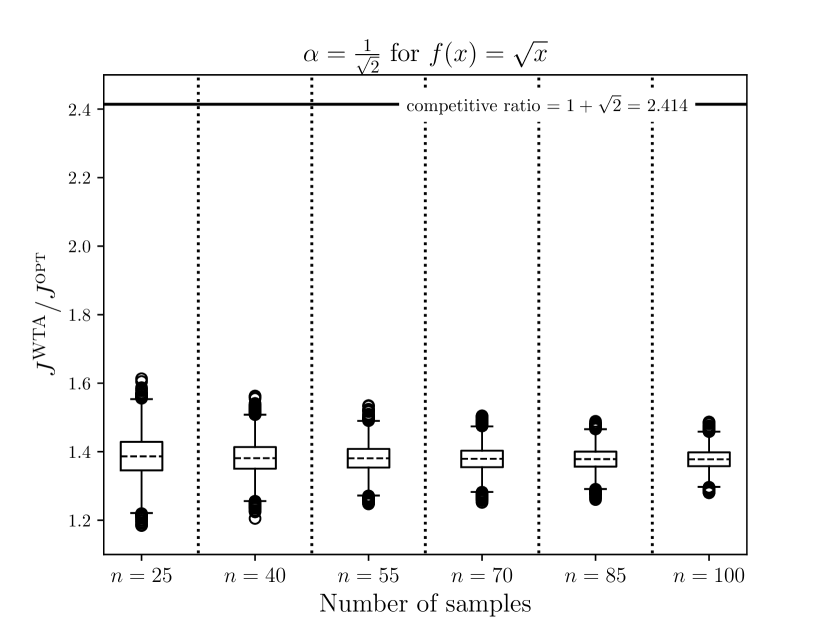
(a)

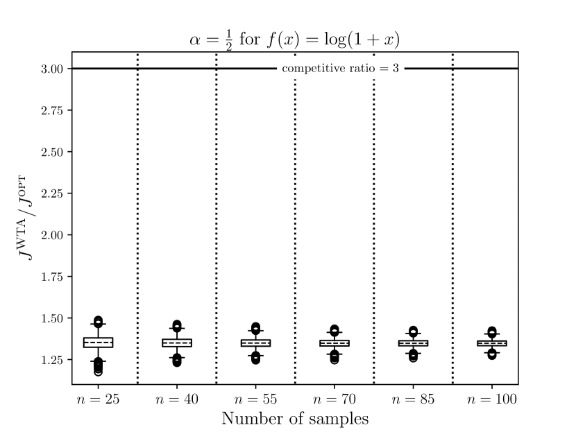
(b)

Figure 3: Performance of WTA over a varying number of samples. We use a Poisson process with rate $\lambda=2$ to generate $n$ arrivals. The value of $\alpha$ for WTA is set based on the “optimal” value given by Corollary 4.4(iii). We plot the results over $10000$ trials for each value of $n$.

In Fig. 3, we show the performance of WTA over a varying number of arrivals $n$ for two different cost functions: $f(x)=\sqrt{x}$ in Fig. 3(a) and $f(x)=\log(1+x)$ in Fig. 3(b). In both cases, we generate the arrivals using a time-homogeneous Poisson process with a (constant) rate $\lambda=2$. For $f(x)=\sqrt{x}$, we have $\Gamma=\inf_{x\in\mathbb{N}}\frac{f(2x)}{f(x)}=\sqrt{2}$, and we use $\alpha=\frac{1}{\sqrt{2}}$ as suggested by Corollary 4.4(iii). Likewise, we have $\Gamma=1$ for $f(x)=\log(1+x)$ and so we use $\alpha=\frac{1}{2}$. For each value of $n$, we generate the arrivals $10000$ times and compute $\frac{J^{\textsc{WTA}}}{J^{\textsc{opt}}}$ for each instance ($J^{\textsc{opt}}$ can be calculated using Alg. 1). The distribution of $\frac{J^{\textsc{WTA}}}{J^{\textsc{opt}}}$ is then shown in Fig. 3.

We can see that in both Fig. 3(a) and Fig. 3(b), there is considerable gap between the maximum value of $\frac{J^{\textsc{WTA}}}{J^{\textsc{opt}}}$ and the competitive ratio. While Corollary 4.4(iii) guarantees that the value of $\frac{J^{\textsc{WTA}}}{J^{\textsc{opt}}}$ would never be more than the competitive ratio, it seems to be the case that a tighter bound might be possible for WTA. Further, we can also see that the distribution of $\frac{J^{\textsc{WTA}}}{J^{\textsc{opt}}}$ concentrates around a certain value as the value of $n$ increases. Note, however, that this does not reduce the competitive ratio for large values of $n$. We can repeat an $n=25$ instance $4$ times (with an appropriate gap between the repetitions) to get an instance with the same ratio of $\frac{J^{\textsc{WTA}}}{J^{\textsc{opt}}}$ for $n=100$. However, such “repeated” instances are unlikely to occur when the arrivals follow a Poisson distribution.

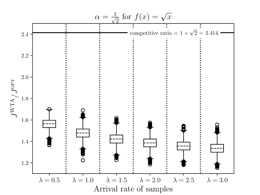
(a)

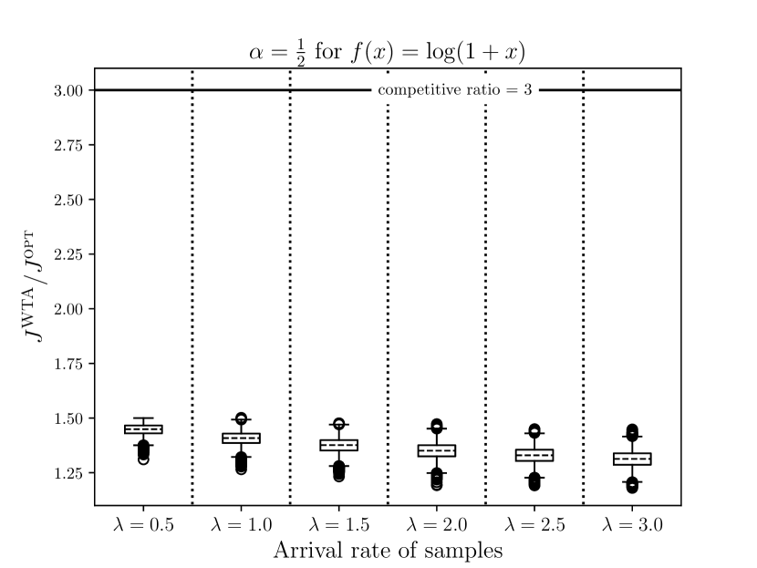
(b)

Figure 4: Performance of WTA over a varying arrival rate of samples. We use a Poisson process with rate $\lambda$ to generate $n=30$ arrivals. The value of $\alpha$ for WTA is set based on the “optimal” value given by Corollary 4.4(iii). We plot the results over $10000$ trials for each value of $\lambda$.

In Fig. 4, we repeat the experiment of Fig. 3, but we fix the value of $n$ to $30$, and instead vary the value of $\lambda$. We observe that the distribution of $\frac{J^{\textsc{WTA}}}{J^{\textsc{opt}}}$ trends downward as $\lambda$ increases in both Fig. 4(a) and Fig. 4(b). This is intuitively reasonable since a very high rate suggests that waiting for samples is better than testing too soon since a new sample is probably just around the corner (due to the high rate). Since WTA waits sufficiently long to give a constant competitive ratio for any possible set of arrival times, the algorithm performs very well when the rate is high. However, since the arrivals are stochastic and any possible set of arrival times have a non-zero probability density, the “competitive ratio” is the same in all these cases.

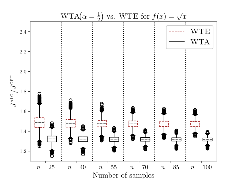
(a)

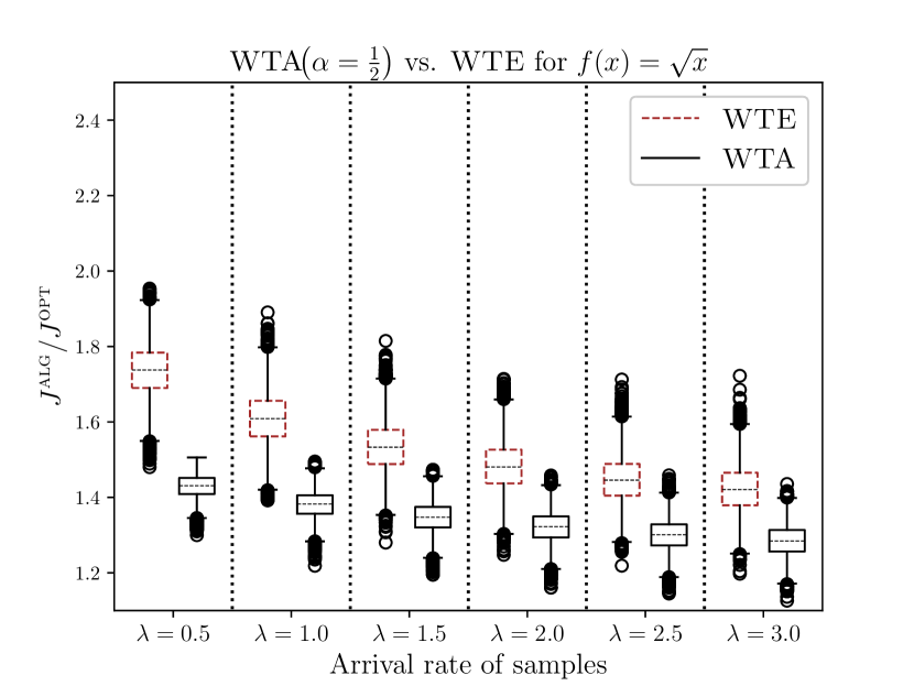
(b)

Figure 5: Comparison of the performance of WTA with $\alpha=\frac{1}{2}$ against WTE (Bhimaraju and Varshney 2022). We use $\lambda=2$ for Fig. 5(a) and $n=30$ for Fig. 5(b), and plot the results over $10000$ trials for each value of $n$ and $\lambda$.

In Fig. 5, we compare the performance of WTA (with $\alpha=\frac{1}{2})$ against WTE (Bhimaraju and Varshney 2022). We vary the value of $n$ in Fig. 5(a) and the rate $\lambda$ in Fig. 5(b). The cost function is $f(x)=\sqrt{x}$ in both cases. Recall that WTA with $\alpha=1$ reduces to WTE. We choose $\alpha=\frac{1}{2}$ because that is the function-agnostic value suggested by Corollary 4.4(i). Additionally, as we see subsequently in Fig. 6, this choice turns out to be better experimentally than $\alpha=\frac{1}{\sqrt{2}}$, which has the best (theoretical) competitive ratio. Fig. 5(a) and Fig. 5(b) show that $\textsc{WTA}\left(\alpha=\frac{1}{2}\right)$ outperforms WTE for all values of $n$ and $\lambda$. As we see in Fig. 5(b), the gains are particularly large for small values of $\lambda$, where the distribution of $\frac{J^{\textsc{WTA}}}{J^{\textsc{opt}}}$ is much lower than the distribution of $\frac{J^{\textsc{WTE}}}{J^{\textsc{opt}}}$. Fig. 6(a) suggests that $\textsc{WTA}\big{(}\alpha=\frac{1}{\sqrt{2}}\big{)}$ is likely to outperform WTE as well, but by a smaller margin than $\textsc{WTA}\left(\alpha=\frac{1}{2}\right)$.

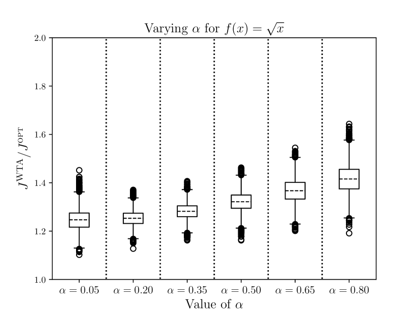
(a)

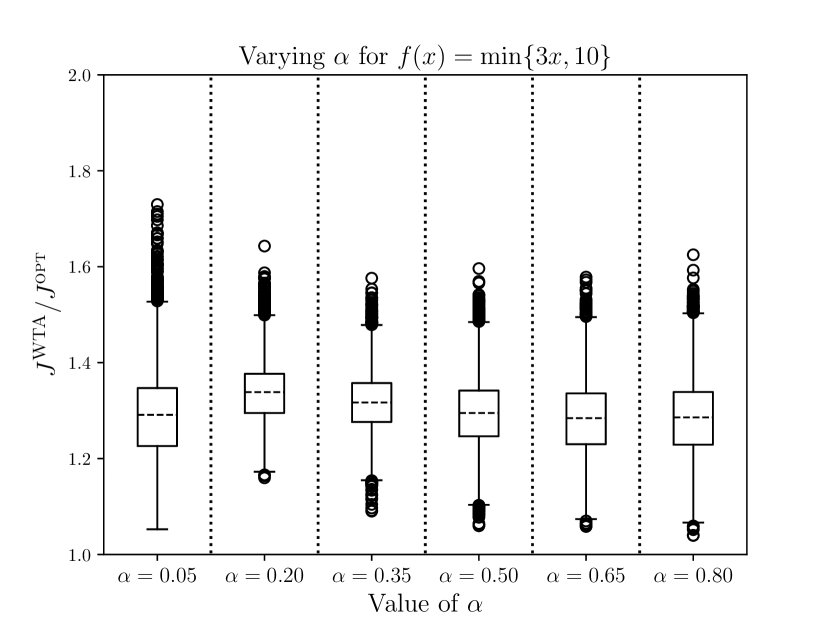
(b)

Figure 6: Performance of WTA for different values of $\alpha$. We use $\lambda=2$ and $n=30$ for all values of $\alpha$, and plot the results over $10000$ trials.

In Fig. 6, we vary the value of $\alpha$ while fixing $n=30$ and $\lambda=2$. Fig. 6(a) uses the cost function $f(x)=\sqrt{x}$. For the worst-case performance, we see in Fig. 6(a) that it improves from $\alpha=0.05$ to $\alpha=0.2$ while worsening for increasing values of $\alpha$. However, for some outlier instances, $\alpha=0.05$ performs better. This is not surprising since if the arrivals are sufficiently spaced apart, the optimal schedule tests them independently, which corresponds to $\alpha=0$. We also observe that for $f(x)=\sqrt{x}$, the value of $\alpha$ that has the best (theoretical) competitive ratio according to Corollary 4.4, i.e., $\alpha=\frac{1}{\sqrt{2}}$, is not the best practical choice. While $f(x)=\log(1+x)$ exhibits similar trends, we omit that function and instead use $f(x)=\min\{3x,10\}$ in Fig. 6(b), which has more interesting behavior. Here, we see that one of the best empirical performances is for $\alpha=\frac{1}{2}$, which also has the best theoretical guarantee. We also see that $\alpha=0.65$ performs just as well, perhaps a little better for some outlier instances.

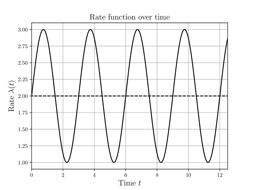
(a)

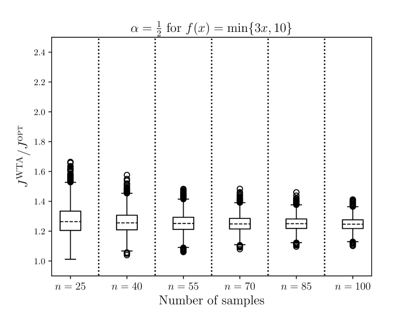
(b)

Figure 7: Performance of WTA for different values of $n$ with a time-inhomogenous arrival rate $\lambda(t)$. We use $\alpha=\frac{1}{2}$ which is the “optimal” choice for $f(x)=\min\{3x,10\}$ according to Corollary 4.4(iii) and plot the results over $10000$ trials.

While the arrivals so far have been homogeneous (constant-rate) Poisson processes, Fig. 7 considers a time-inhomogeneous Poisson process. We use the rate function $\lambda(t)=2+\sin\left(\frac{2\pi}{3}t\right)$ shown in Fig. 7(a). We use the cost function $f(x)=\min\{3x,10\}$ from Fig. 6(b). Fig. 7(b) shows the performance of WTA with $\alpha=\frac{1}{2}$ for the arrival process $\lambda(t)$ for a varying $n$. We see a trend similar to Fig. 3, where the distribution of $\frac{J^{\textsc{WTA}}}{J^{\textsc{opt}}}$ concentrates around a certain value as $n$ increases. Note that since $\alpha=\frac{1}{2}$ and $\Gamma=1$, the competitive ratio guaranteed by Corollary 4.4 is $3$.

Real-world data

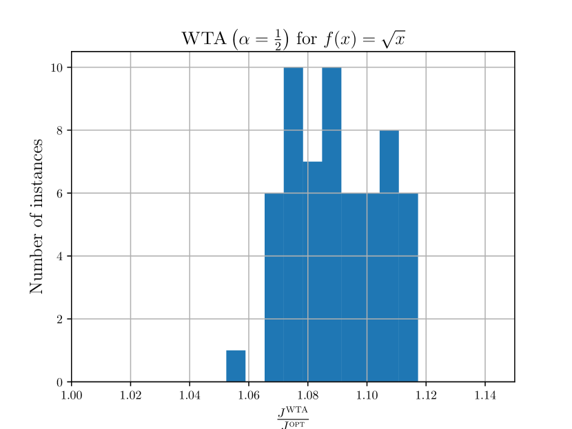
(a)

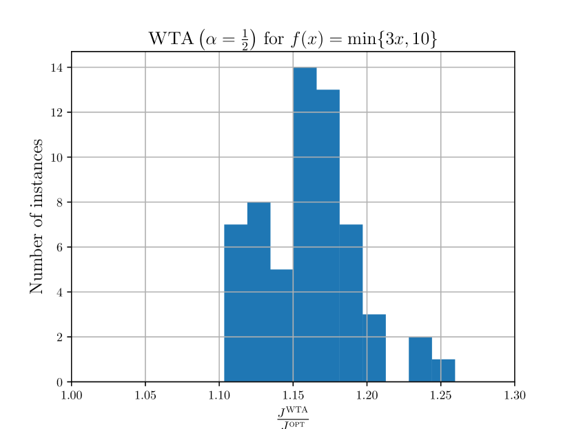
(b)

Figure 8: Performance of WTA with $\alpha=\frac{1}{2}$ over the arrival data from Bishop et al. (2018). In Fig. 8(a) we use the processing cost function $f(x)=\sqrt{x}$ and in Fig. 8(b) we use the function $f(x)=\min\{3x,10\}$. The best schedule is computed using OSP and we plot the histogram of $\frac{J^{\textsc{WTA}}}{J^{\textsc{opt}}}$ over the $60$ instances in the data.

We use the customer arrival data at $3$ banks over $4$ weeks collected by Bishop et al. (2018). We consider each day of each week as a problem instance, giving us a total of $3\times 4\times 5=60$ instances over which we report the statistics. For each instance, customers arrive from $8$ AM to $3$ PM (i.e., over a period of $7$ hours), and the average number of arrivals per day was $874.9$. We can see in Fig. 8 that the schedule given by WTA is very close to the optimal schedule. For all the instances considered here, the cost of the WTA schedule was less than a factor $1.3$ away from the optimal. We also observe that we have (marginally) better performance in Fig. 8(a) for $f(x)=\sqrt{x}$ compared to $f(x)=\min\{3x,10\}$ in Fig. 8(b).

7 Conclusions and Future Research Directions

In this work, we give a competitive algorithm for the dynamic batching of samples that arrive over time. We consider the average wait time of the samples plus the average per-sample processing cost as the objective to minimize. We first give a polynomial-time algorithm that computes the optimal offline schedule. We then consider the online problem and devise constant competitive algorithms for general concave processing cost functions. We also give a lower bound on the competitive ratio that no online algorithm can beat.

However, there is still a gap between the competitive ratio guaranteed by our online algorithm and the proposed lower bound. One avenue for future research is to close this gap. This may be pursued by (i) using more precise analysis to show that WTA has a better competitive ratio, (ii) improving the lower bound by showing no online algorithm can achieve a better competitive ratio, or (iii) develop new algorithms better than WTA and show an improved competitive ratio. Developing randomized algorithms that achieve a lower competitive ratio in expectation would be another interesting research direction. Finally, the competitive ratios that we obtained in this work hold for any adversarial arrival sequence. However, as we observed in our numerical experiments, for stochastic arrivals, one might be able to leverage additional statistics of the arrivals sequence to show improved competitive ratios for the WTA. We believe all these have much potential for future research.

This work was supported in part by NSF grant ECCS-2033900, and the Center for Pathogen Diagnostics through the ZJU-UIUC Dynamic Engineering Science Interdisciplinary Research Enterprise (DESIRE).

8 Proof of Claim 1

For proving part (i), we use induction on $y$. Using Assumption 2, we can write

$$f(x+1)-f(x) \leq f(x)-f(x-1)$$

$$\leq f(x-1)-f(x-2)$$

$$\leq\cdots\leq f(1)-f(0)=f(1).$$

This gives us $f(x+1)\leq f(x)+f(1)$, which is the base case for $y=1$. Now assume that part (i) of Claim 1 is true for $y=k-1$, and consider

$$f(x+k)-f(x+k-1) \leq f(x+k-1)-f(x+k-2)$$

$$\leq f(x+k-2)-f(x+k-3)$$

$$\leq\cdots\leq f(k)-f(k-1).$$

This gives us $f(x+k)\leq f(x+k-1)+f(k)-f(k-1)$, but since part (i) is true for $y=k-1$, using $f(x+k-1)\leq f(x)+f(k-1)$, we get

$$f(x+k)\leq f(x)+f(k).$$

This completes the induction and so the assertion holds for all $y\in\mathbb{N}$. Since we have made no assumptions on $x$, the statement is thus true for all $x,y\in\mathbb{N}$.

For proving part (ii) of Claim 1, it will be helpful to define a real extension of $f(\cdot)$ using linear interpolation. Let $\tilde{f}:\mathbb{R}^{+}\cup\{0\}\mapsto\mathbb{R}^{+}\cup\{0\}$ be defined as follows:

$$\tilde{f}(x)=\begin{cases}f(x)\qquad\qquad\qquad&\text{if}\ x\in\mathbb{N}\cup\{0\},\\ \left(x-\lfloor x\rfloor\right)f\left(\lceil x\rceil\right)+\left(\lceil x\rceil-x\right)f\left(\lfloor x\rfloor\right)\ &\text{else},\end{cases}$$

where $\lceil\cdot\rceil$ and $\lfloor\cdot\rfloor$ are the integer ceiling and floor functions, respectively. It follows directly that $\tilde{f}$ is continuous and non-decreasing. Further, since the slope at $x\notin\mathbb{N}\cup\{0\}$ is $f\left(\lceil x\rceil\right)-f\left(\lfloor x\rfloor\right)$, which can only decrease with $x$ from our assumptions on $f(\cdot)$, $\tilde{f}(\cdot)$ is a concave function in its domain. This gives us

$$\theta f(x)+(1-\theta)f(y) =\theta\tilde{f}(x)+(1-\theta)\tilde{f}(y)$$

$$\leq\tilde{f}(\theta x+(1-\theta)y)$$

$$\leq\tilde{f}\left(\lceil\theta x+(1-\theta)y\rceil\right)$$

$$=f\left(\lceil\theta x+(1-\theta)y\rceil\right),$$

which completes the proof of part (ii) of Claim 1.

For part (iii), let us first observe that $\Gamma\in[1,2]$. This is because the monotonicity of $f$ implies $f(2x)\geq f(x)$ (giving us $\Gamma\geq 1$), and Claim 1(ii) with $x=2x$, $y=0$, and $\theta=\frac{1}{2}$ yields $f(2x)\leq 2f(x)$ (giving us $\Gamma\leq 2$). Since $\Gamma\in[1,2]$, we have $\frac{2}{\Gamma}\geq 1$ for any function $f$, and thus Claim 1(iii) holds when either $x=0$ or $y=0$ (but not both).

So we are just left with the case where $x\in\mathbb{N}$ and $y\in\mathbb{N}$ (neither is $0$). Applying Claim 1 with $x=2x$, $y=2y$, and $\theta=\frac{1}{2}$ gives

$$\frac{1}{2}f(2x)+\frac{1}{2}f(2y)\leq f(x+y)\leq f(x)+f(y),$$

where the last inequality follows from Claim 1(i). This gives us

$$\frac{f(x)+f(y)}{f(x+y)}\leq\frac{f(x)+f(y)}{\frac{1}{2}f(2x)+\frac{1}{2}f(2y)}=2\frac{f(x)+f(y)}{f(2x)+f(2y)}.$$

The fraction on the right side is a linear combination of $\frac{f(x)}{f(2x)}$ and $\frac{f(y)}{f(2y)}$ (since $x,y\neq 0$), so we can write

$$\frac{f(x)+f(y)}{f(x+y)}\leq 2\max\left\{\frac{f(x)}{f(2x)},\frac{f(y)}{f(2y)}\right\}.$$

From the definition of $\Gamma$, we have $\frac{f(x)}{f(2x)}\leq\frac{1}{\Gamma}$ and $\frac{f(y)}{f(2y)}\leq\frac{1}{\Gamma}$, which gives Claim 1(iii).

9 Proof of Claim 2

We prove this claim by showing that any (optimal) schedule can be converted, without increasing the cost, into one where the following property is true: if there is a test at some $t=s^{\textsc{opt}}_{j}$, then $u^{\textsc{opt}}_{t}=0$.

In an optimal schedule opt, assume only $n_{1}$ samples are tested at some time $t$, while $n_{2}$ samples, already available at $t$, are tested in a different batch along with $n_{\text{new}}$ samples (all released at times after $t$) at some time $t+\Delta t$. We prove this claim by showing that at least one of the following does not increase the cost:

• test the $n_{1}+n_{2}$ samples together at time $t$, or

• test all the $n_{1}+n_{2}+n_{\text{new}}$ samples together at time $t+\Delta t$.

Let us assume the contrary (which will lead us to a contradiction): both the options above strictly increase the cost. Note that the waiting time of the $n_{\text{new}}$ samples is the same in all cases. Further, the waiting time and testing costs of samples that are not in these $n_{1}+n_{2}+n_{\text{new}}$ samples are the same in all the cases. Considering only the terms that are different, the above two cases imply

$$f(n_{1})+f(n_{2}+n_{\text{new}})+n_{2}\Delta t <f(n_{1}+n_{2})+f(n_{\text{new}}),$$

$$f(n_{1})+f(n_{2}+n_{\text{new}})+n_{2}\Delta t <f(n_{1}+n_{2}+n_{\text{new}})+(n_{1}+n_{2})\Delta t.$$

These inequalities give us

$$\Delta t <\frac{f(n_{1}+n_{2})+f(n_{\text{new}})-f(n_{1})-f(n_{2}+n_{\text{new}})}{n_{2}},$$

$$\Delta t >\frac{f(n_{1})+f(n_{2}+n_{\text{new}})-f(n_{1}+n_{2}+n_{\text{new}})}{n_{1}}.$$

Putting the two together, we get

$$\frac{f(n_{1})+f(n_{2}+n_{\text{new}})-f(n_{1}+n_{2}+n_{\text{new}})}{n_{1}}\qquad\qquad\qquad\qquad$$

$$\qquad<\frac{f(n_{1}+n_{2})+f(n_{\text{new}})-f(n_{1})-f(n_{2}+n_{\text{new}})}{n_{2}}.$$

Rearranging the terms gives us

$$f(n_{1})+f(n_{2}+n_{\text{new}})< \tfrac{n_{1}}{n_{1}+n_{2}}f(n_{1}+n_{2})$$

$$+\tfrac{n_{1}}{n_{1}+n_{2}}f(n_{\text{new}}) +\tfrac{n_{2}}{n_{1}+n_{2}}f(n_{1}+n_{2}+n_{\text{new}}).$$ (15)

Using Claim 1(ii) with $\theta=\frac{n_{1}}{n_{1}+n_{1}}$, $x=n_{1}+n_{2}$, and $y=0$ gives

$$\frac{n_{1}}{n_{1}+n_{2}}f(n_{1}+n_{2})\leq f(\lceil n_{1}\rceil)=f(n_{1}).$$ (16)

With $\theta=\frac{n_{1}}{n_{1}+n_{2}}$, $x=n_{\text{new}}$, and $y=n_{1}+n_{2}+n_{\text{new}}$, we get

$$\frac{n_{1}}{n_{1}+n_{2}}f(n_{\text{new}}) +\frac{n_{2}}{n_{1}+n_{2}}f(n_{1}+n_{2}+n_{\text{new}})$$

$$\leq f(\lceil n_{2}+n_{\text{new}}\rceil)=f(n_{2}+n_{\text{new}}).$$ (17)

Substituting (16) and (17) into (15) gives

$$f(n_{1})+f(n_{2}+n_{\text{new}})<f(n_{1})+f(n_{2}+n_{\text{new}}),$$

which is a contradiction.

10 Linear program for the offline problem

Since we formulated the batch-scheduling problem as one of finding the minimum-weight path in a graph, we can write it as an integer linear program. However, as we show, we do not need to solve with integral constraints, and a relaxed version of the program over a convex polyhedron gives the same cost as the integer program. More concretely, consider the problem of finding the minimum-weight path in the graph defined in Sec. 3 and define the binary variables $x_{i,j}\in\{0,1\}$ for $i<j$ with $i\in\{1,2,\ldots,n\}$ and $j\in\{2,3,\ldots,n+1\}$. Each batching schedule corresponds to an assignment of $0$s and $1$s to all $x_{i,j}$, and we interpret this as $x_{i,j}=1$ if and only if the arrivals $\{i,i+1,\ldots,j-1\}$ are processed in a single batch. Additionally, arrivals before $i$ and after $j-1$ are not part of this batch. Let the edge weights $e_{i,j}$ be defined as we did in Sec. 3 for $e_{ij}$, i.e., $e_{i,j}:=f(j-i)+\sum_{k=i}^{j-1}(a_{j-1}-a_{k})$.

Consider the following integer linear program.

$$\underset{x_{i,j}\in\{0,1\}}{\text{minimize}} \quad\frac{1}{n}\sum_{i<j}x_{i,j}e_{i,j}$$ (ILP)

subject to $$\quad\sum_{j=2}^{n+1}x_{1,j}=1\qquad(\text{for}\ i=1),$$

$$\quad\sum_{j=i+1}^{n+1}x_{i,j}=\sum_{j=1}^{i-1}x_{j,i}\quad\text{for all}\ i\in\{2,3,\ldots,n\}.$$

Claim 3

The optimal solution of (ILP), $\{x_{i,j}^{*}\}$, has a cost equal to $J^{\textsc{opt}}$, the cost of the optimal batching schedule. Further, this cost can be achieved by scheduling in such a way that we form a batch of arrivals $\{i,i+1,\ldots,j-1\}$ if and only if $x_{i,j}^{*}=1$. Solving (ILP) results in a solution where this batching gives a valid schedule (i.e., no arrival is assigned to multiple batches, and every arrival is assigned to at least one batch).

Proof 10.1

Proof. We prove this claim in two parts: (i) we show that there is a feasible solution which gives a cost of $J^{\textsc{opt}}$ — this guarantees that the optimal cost is not more than $J^{\textsc{opt}}$; and (ii) we show that any (optimal) solution of (ILP) corresponds to a valid batching schedule. This implies that the optimal solution cannot have a cost less than $J^{\textsc{opt}}$, since the the best possible schedule for the batching problem has a cost of $J^{\textsc{opt}}$.

For part (i), let a best batching schedule (that satisfies Claim 2) be given by the $m$ batches $\mathcal{B}^{\textsc{opt}}_{1},\mathcal{B}^{\textsc{opt}}_{2},\ldots,\mathcal{B}^{\textsc{opt}}_{m}$. For each $\mathcal{B}^{\textsc{opt}}_{k}$, define $p_{k}:=\min\{i:i\in\mathcal{B}^{\textsc{opt}}_{k}\}$ and $q_{k}:=\max\{i:i\in\mathcal{B}^{\textsc{opt}}_{k}\}+1$, and set $x_{p_{k},q_{k}}=1$. Set the remaining $x_{i,j}=0$. From the definition of $e_{i,j}$, we can see that the cost of this schedule is equal to $\frac{1}{n}\sum_{i<j}x_{i,j}e_{i,j}$. To show that this assignment of $0$s and $1$s to $\{x_{i,j}\}$ is feasible, observe the following. Since $\mathcal{B}^{\textsc{opt}}_{1}$ includes the first arrival, the value of $x_{1,\max\{\mathcal{B}^{\textsc{opt}}_{1}\}+1}$ would be set to $1$. Further, no other batch contains the first arrival, so the sum $\sum_{j=2}^{n+1}x_{1,j}$ is equal to $1$. This is sufficient to satisfy the first ($i=1$) constraint. For each $i\in\{2,3,\ldots,n\}$, the only way the right side of the second constraint is nonzero is if the $(i-1)$th arrival was the last arrival of some batch $\mathcal{B}^{\textsc{opt}}_{k}$. In this case, the right side is equal to $1$, but the left side is also equal to $1$ since the $i$th arrival is now the first sample of $\mathcal{B}^{\textsc{opt}}_{k+1}$. So all the constraints are satisfied and this solution is feasible. Thus the optimal cost of (ILP) is not more than $J^{\textsc{opt}}$.

Now we have to prove part (ii). Assume that the solution of (ILP) is $\{x_{i,j}^{*}\}$, and we batch the arrivals into batches $\{i,i+1,\ldots,j-1\}$ if and only if $x_{i,j}^{*}=1$. Fixing an $i=\hat{i}\ (\in\{1,2,\ldots,n\})$ and adding up the constraints for $i=1,2,\ldots,\hat{i}$ gives

$$\sum_{i=1}^{\hat{i}}\sum_{j=i+1}^{n+1}x_{i,j}=1+\sum_{i=1}^{\hat{i}}\sum_{j=1}^{i-1}x_{j,i}.$$

Every $x_{i,j}$ term on the right side in the above equation also occurs on the left side, and cancelling these gives

$$\sum_{i=1}^{\hat{i}}\sum_{j=\hat{i}+1}^{n+1}x_{i,j}=1\quad\forall\ \hat{i}\in\{1,2,\ldots,n\}.$$ (18)

Since $\{x_{i,j}^{*}\}$ (optimally) solves (ILP), it must satisfy (18). Since all $x_{i,j}$ are binary variables, (18) implies for any $\hat{i}$ that there is exactly one $(i,j)$ with $i\leq\hat{i}$ and $j>\hat{i}$ such that $x_{i,j}=1$. So each arrival $\hat{i}$ is assigned to exactly one and only one batch. This proves that the optimal solution $\{x_{i,j}^{*}\}$ always results in a valid batching schedule when we schedule it according to the scheme given in the claim, which concludes the proof.

Solving (ILP) directly using integer linear-programming solvers for large problem instances is intractable due to the integer constraints $x_{i,j}\in\{0,1\}$. However, we can relax these constraints to the convex $x_{i,j}\geq 0$, and it turns out that there is an optimal solution to this (convex) linear program where $x_{i,j}$ is binary. Since the domain of $\{x_{i,j}\geq 0\}$ is a superset of $x_{i,j}\in\{0,1\}$, this solution of the relaxed linear program is thus an optimal solution of (ILP) as well. We state this relaxed program formally as (LP) and the equivalence as Claim 4.

$$\underset{x_{i,j}\geq 0}{\text{minimize}} \quad\frac{1}{n}\sum_{i<j}x_{i,j}e_{i,j}$$ (LP)

subject to $$\quad\sum_{j=2}^{n+1}x_{1,j}=1\qquad(\text{for}\ i=1),$$

$$\quad\sum_{j=i+1}^{n+1}x_{i,j}=\sum_{j=1}^{i-1}x_{j,i}\quad\text{for all}\ i\in\{2,3,\ldots,n\}.$$

Claim 4

There is an optimal solution of (LP), $\{\tilde{x}_{i,j}\}$, that satisfies $\tilde{x}_{i,j}\in\{0,1\}$.

Proof 10.2

Proof. For each constraint in (LP), define the dual variable $\lambda_{i}$ for $i\in\{1,2,\ldots,n\}$. The dual program of (LP), (DP) is given by

$$\underset{\lambda_{i}\in\mathbb{R}}{\text{maximize}} \qquad\lambda_{1}$$ (DP)

subject to $$\quad\lambda_{i}\leq\frac{e_{i,n+1}}{n}\quad\text{for}\ i\in\{1,2,\ldots,n\},$$

$$\quad\lambda_{i}\leq\frac{e_{i,j}}{n}+\lambda_{j}\quad\text{for}\ i<j\ \ (i,j\in\{1,2,\ldots,n\}).$$

We prove Claim 4 by showing that the objective value of a dual-feasible solution is equal to that achieved by a binary solution for the primal program (LP). To see this, define $\lambda_{n+1}:=0$ so we can write both the constraints compactly as

$$\lambda_{i}\leq\frac{e_{i,j}}{n}+\lambda_{j}\quad\text{for}\ i<j\ \ (i,j\in\{1,2,\ldots,n+1\}).$$

Since we are maximizing $\lambda_{1}$ in (DP), it will be equal to the right side of one of the inequalities containing $\lambda_{1}$:

$$\lambda_{1}=\min_{j\in\{2,3,\ldots,n+1\}}\left\{\frac{e_{1,j}}{n}+\lambda_{j}\right\}.$$

This implies that for the maximum value of $\lambda_{1}$, we need to find the maximum values of $\lambda_{j}$ for $j\in\{2,3,\ldots,n\}$ (the value of $\lambda_{n+1}$ is fixed to $0$). This suggests a natural recursion for computing the optimal value of $\lambda_{1}$. Starting with the base case $\lambda_{n+1}=0$, we have for $i\in\{n,n-1,\ldots,1\}$:

$$\lambda_{i}=\min_{j\in\{i+1,i+2,\ldots,n+1\}}\left\{\frac{e_{i,j}}{n}+\lambda_{j}\right\}.$$ (19)

Let $r_{i}$ denote the index where the minimum in (19) occurs:

$$r_{i}=\arg\min_{j\in\{i+1,i+2,\ldots,n+1\}}\left\{\frac{e_{i,j}}{n}+\lambda_{j}\right\}.$$

Use the following procedure to assign values to $\{\tilde{x}_{i,j}\}$:

1:Initialize $i\leftarrow 1$ and $\tilde{x}_{p,q}\leftarrow 0$ for all $p<q$

2:while $i\leq n$ do

3:     $\tilde{x}_{i,r_{i}}\leftarrow 1$

4:     $i\leftarrow r_{i}$

5:end while

From the definition of $r_{i}$, we have

$$\lambda_{i}=\frac{e_{i,r_{i}}}{n}+\lambda_{r_{i}},$$

which implies

$$\lambda_{1}=\frac{1}{n}\sum_{i=1}^{n}\sum_{j=i+1}^{n+1}\tilde{x}_{i,j}e_{i,j}.$$ (20)

Thus there is a dual-feasible solution which has the same cost as a binary solution for the primal program (LP). We now just have to show that this binary solution satisfies all the constraints of (LP) to conclude the proof. The first constraint of (LP) is satisfied since $\tilde{x}_{1,r_{1}}=1$ and $\tilde{x}_{1,j}=0$ for $j\neq r_{1}$. Further, observe that $\tilde{x}_{i,j}$ is nonzero if and only if $i$ and $j$ both occur in the $\{r_{1},r_{r_{1}},r_{r_{r_{1}}},\ldots\}$ sequence, and $j=r_{i}$. This ensures that for each element in this sequence, there is exactly one term in the second constraint of (LP) that is $1$. All other terms are $0$ guaranteeing that the constraint is valid for all $i$, and thus $\{\tilde{x}_{i,j}\}$ is a primal-feasible solution. So there is a feasible binary solution for the primal which has an objective equal to a feasible solution for the dual (by (20)), which means that these are the optimal solutions for both the primal and the dual (Boyd and Vandenberghe 2004).

Together with Claim 3, Claim 4 implies that we can solve (LP) to find the optimal batching schedule. This can be done using any off-the-shelf linear-program solver since (LP) is just a standard linear program. We also observe in the proof of Claim 4 that solving the dual program bears a lot of similarity to how the minimum-weight path is computed once we have a topologically sorted order of the vertices in the graph. The recursion in (19) is essentially the same dynamic program that computes the minimum-weight path via topological sorting (Cormen et al. 2022).

References

- Acemoglu et al. (2021) Acemoglu D, Fallah A, Giometto A, Huttenlocher D, Ozdaglar A, Parise F, Pattathil S (2021) Optimal adaptive testing for epidemic control: combining molecular and serology tests. arXiv:2101.00773 [eess.SY].
- Ahn et al. (2021) Ahn S, Chen W, Özgür A (2021) Adaptive group testing on networks with community structure. Proc. IEEE Int. Symp. Inf. Theory (ISIT), 1242–1247.
- Albers and Fujiwara (2007) Albers S, Fujiwara H (2007) Energy-efficient algorithms for flow time minimization. ACM Trans. Algorithms 3(4):49–es.
- Aldridge (2018) Aldridge M (2018) Individual testing is optimal for nonadaptive group testing in the linear regime. IEEE Trans. Inf. Theory 65(4):2058–2061.
- Aldridge et al. (2014) Aldridge M, Baldassini L, Johnson O (2014) Group testing algorithms: Bounds and simulations. IEEE Trans. Inf. Theory 60(6):3671–3687.
- Aldridge et al. (2019) Aldridge M, Johnson O, Scarlett J (2019) Group testing: An information theory perspective. Found. Trends Commun. Inf. Theory 15(3-4):196–392.
- Arasli and Ulukus (2023) Arasli B, Ulukus S (2023) Group testing with a graph infection spread model. Information 14(1):48.
- Baldassini et al. (2013) Baldassini L, Johnson O, Aldridge M (2013) The capacity of adaptive group testing. Proc. IEEE Int. Symp. Inf. Theory (ISIT), 2676–2680.
- Bansal et al. (2010) Bansal N, Pruhs K, Stein C (2010) Speed scaling for weighted flow time. SIAM J. Comput. 39(4):1294–1308.
- Bar-Lev et al. (2007) Bar-Lev SK, Parlar M, Perry D, Stadje W, Van der Duyn Schouten FA (2007) Applications of bulk queues to group testing models with incomplete identification. Eur. J. Oper. Res. 183(1):226–237.
- Bhimaraju and Varshney (2022) Bhimaraju A, Varshney LR (2022) Scheduling group tests over time. Proc. IEEE Int. Symp. Inf. Theory (ISIT), 886–891.
- Bishop et al. (2018) Bishop SA, Okagbue HI, Oguntunde PE, Opanuga AA, Odetunmibi OA (2018) Survey dataset on analysis of queues in some selected banks in Ogun State, Nigeria. Data in Brief 19:835–841.
- Boyd and Vandenberghe (2004) Boyd SP, Vandenberghe L (2004) Convex Optimization (Cambridge University Press).
- Chakravarthy et al. (2021) Chakravarthy SR, Shruti, Rumyantsev A (2021) Analysis of a queueing model with batch Markovian arrival process and general distribution for group clearance. Methodol. Comput. Appl. Probab. 23(4):1551–1579.
- Chakravarty et al. (1982) Chakravarty AK, Orlin JB, Rothblum UG (1982) A partitioning problem with additive objective with an application to optimal inventory groupings for joint replenishment. Oper. Res. 30(5):1018–1022.
- Chan et al. (2014) Chan CL, Jaggi S, Saligrama V, Agnihotri S (2014) Non-adaptive group testing: Explicit bounds and novel algorithms. IEEE Trans. Inf. Theory 60(5):3019–3035.
- Claeys et al. (2013) Claeys D, Steyaert B, Walraevens J, Laevens K, Bruneel H (2013) Tail probabilities of the delay in a batch-service queueing model with batch-size dependent service times and a timer mechanism. Comput. Oper. Res. 40(5):1497–1505.
- Claeys et al. (2010) Claeys D, Walraevens J, Laevens K, Bruneel H (2010) A queueing model for general group screening policies and dynamic item arrivals. Eur. J. Oper. Res. 207(2):827–835.
- Cormen et al. (2022) Cormen TH, Leiserson CE, Rivest RL, Stein C (2022) Introduction to Algorithms (MIT Press), fourth edition.
- Deb and Serfozo (1973) Deb RK, Serfozo RF (1973) Optimal control of batch service queues. Adv. Appl. Probab. 5(2):340–361.
- Devanur and Huang (2018) Devanur NR, Huang Z (2018) Primal dual gives almost optimal energy-efficient online algorithms. ACM Trans. Algorithms 14(1):1–30.
- Doger and Ulukus (2022) Doger M, Ulukus S (2022) Dynamical Dorfman testing with quarantine. Proc. Conf. Inf. Sci. Syst. (CISS).
- Dorfman (1943) Dorfman R (1943) The detection of defective members of large populations. Ann. Math. Stat. 14(4):436–440.
- Edmonds (2000) Edmonds J (2000) Scheduling in the dark. Theor. Comput. Sci. 235(1):109–141.
- Feng and Niazadeh (2022) Feng Y, Niazadeh R (2022) Batching and optimal multi-stage bipartite allocations. arXiv:2211.16581 [cs.DS].
- Gandikota et al. (2019) Gandikota V, Grigorescu E, Jaggi S, Zhou S (2019) Nearly optimal sparse group testing. IEEE Trans. Inf. Theory 65(5):2760–2773.
- Garey and Johnson (1975) Garey MR, Johnson DS (1975) Complexity results for multiprocessor scheduling under resource constraints. SIAM J. Comput. 4(4):397–411.
- Graham (1966) Graham RL (1966) Bounds for certain multiprocessing anomalies. Bell Syst. Tech. J. 45(9):1563–1581.
- Hall et al. (1997) Hall LA, Schulz AS, Shmoys DB, Wein J (1997) Scheduling to minimize average completion time: Off-line and on-line approximation algorithms. Math. Oper. Res. 22(3):513–544.
- Lyft (2016) Lyft (2016) Matchmaking in Lyft Line. https://eng.lyft.com/matchmaking-in-lyft-line-9c2635fe62c4, Accessed on 2023-09-01.
- Neuts and Chandramouli (1987) Neuts MF, Chandramouli Y (1987) Statistical group testing with queueing involved. Queueing Syst. 2(1):19–39.
- Nikolopoulos et al. (2021a) Nikolopoulos P, Srinivasavaradhan SR, Guo T, Fragouli C, Diggavi S (2021a) Group testing for connected communities. Proc. Int. Conf. Artif. Intell. Stat. (AISTATS), 2341–2349.
- Nikolopoulos et al. (2021b) Nikolopoulos P, Srinivasavaradhan SR, Guo T, Fragouli C, Diggavi S (2021b) Group testing for overlapping communities. Proc. IEEE Int. Conf. Commun. (ICC), 1–7.
- Pruhs (2007) Pruhs K (2007) Competitive online scheduling for server systems. ACM SIGMETRICS Perform. Eval. Rev. 34(4):52–58.
- Ross (2023) Ross SM (2023) Introduction to Probability Models (Academic Press), thirteenth edition.
- Ruszinkó (1994) Ruszinkó M (1994) On the upper bound of the size of the -cover-free families. J. Comb. Theory, Ser. A 66(2):302–310.
- Scarlett and Johnson (2020) Scarlett J, Johnson O (2020) Noisy non-adaptive group testing: A (near-) definite defectives approach. IEEE Trans. Inf. Theory 66(6):3775–3797.
- Smith (1776) Smith A (1776) An Inquiry into the Nature and Causes of the Wealth of Nations (W. Strahan and T. Cadell).
- Srinivasavaradhan et al. (2021) Srinivasavaradhan SR, Nikolopoulos P, Fragouli C, Diggavi S (2021) An entropy reduction approach to continual testing. Proc. IEEE Int. Symp. Inf. Theory (ISIT), 611–616.
- Uber (2023) Uber (2023) How does Uber match riders with drivers? https://www.uber.com/us/en/marketplace/matching/, Accessed on 2023-09-01.
- Ullman (1975) Ullman JD (1975) NP-complete scheduling problems. J. Comput. Sys. Sci. 10(3):384–393.
- Vaze and Nair (2022) Vaze R, Nair J (2022) Speed scaling with multiple servers under a sum-power constraint. ACM SIGMETRICS Perform. Eval. Rev. 49(3):45–50.
- Wei et al. (2021) Wei L, Kapuscinski R, Jasin S (2021) Shipping consolidation across two warehouses with delivery deadline and expedited options for e-commerce and omni-channel retailers. Manuf. & Serv. Oper. Manage. 23(6):1634–1650.
- Xie et al. (2022) Xie Y, Ma W, Xin L (2022) The benefits of delay to online decision-making. Available at SSRN: https://ssrn.com/abstract=4248326 .
- Zhang et al. (2017) Zhang L, Hu T, Min Y, Wu G, Zhang J, Feng P, Gong P, Ye J (2017) A taxi order dispatch model based on combinatorial optimization. Proc. ACM SIGKDD Int. Conf. Knowledge Discovery Data Mining, 2151–2159.