Algorithmic Recourse for Anomaly Detection in Multivariate Time Series

Abstract.

Anomaly detection in multivariate time series has received extensive study due to the wide spectrum of applications. An anomaly in multivariate time series usually indicates a critical event, such as a system fault or an external attack. Therefore, besides being effective in anomaly detection, recommending anomaly mitigation actions is also important in practice yet under-investigated. In this work, we focus on algorithmic recourse in time series anomaly detection, which is to recommend fixing actions on abnormal time series with a minimum cost so that domain experts can understand how to fix the abnormal behavior. To this end, we propose an algorithmic recourse framework, called RecAD, which can recommend recourse actions to flip the abnormal time steps. Experiments on two synthetic and one real-world datasets show the effectiveness of our framework.

1. Introduction

Multivariate time series is a collection of observations that are recorded chronologically and have correlations in time. Due to the ubiquitous of multivariate time series, anomaly detection in time series data has received a large number of studies (Blázquez-García et al., 2021) and has a wide spectrum of applications, such as detecting abnormal behaviors in online services (Ren et al., 2019; Shipmon et al., 2017).

Algorithmic recourse is to provide recommendations to flip unfavorable outcomes by automated decision-making systems with minimum cost (Karimi et al., 2022). For example, if a loan application is denied by a system, algorithmic recourse is to figure out how to flip the decision (loan approved) with minimum cost. In the area of time series anomaly detection, after receiving an alert about a potential abnormal behavior detected by an anomaly detection model, algorithmic recourse is to predict recourse actions to fix such abnormal behavior.

For example, Figure 1 presents the usage of two control nodes, nodes 117 and 124, in an OpenStack testbed (Nedelkoski et al., 2020). Each node’s performance includes the CPU time spent on running the user’s programs and memory usage. When an anomaly detection model triggers an anomaly alert (the red area in the top figure), a recourse action, which aims to flip the abnormal behavior, is recommended to free up memory usage on node 124. After taking the recourse action (the green area in the bottom figure), the system returns to normal (dashed lines in the bottom figure). Therefore, if there is abnormal behavior in a distributed system detected by an anomaly detection model, algorithmic recourse can help the domain expert quickly fix the issue with minimum cost.

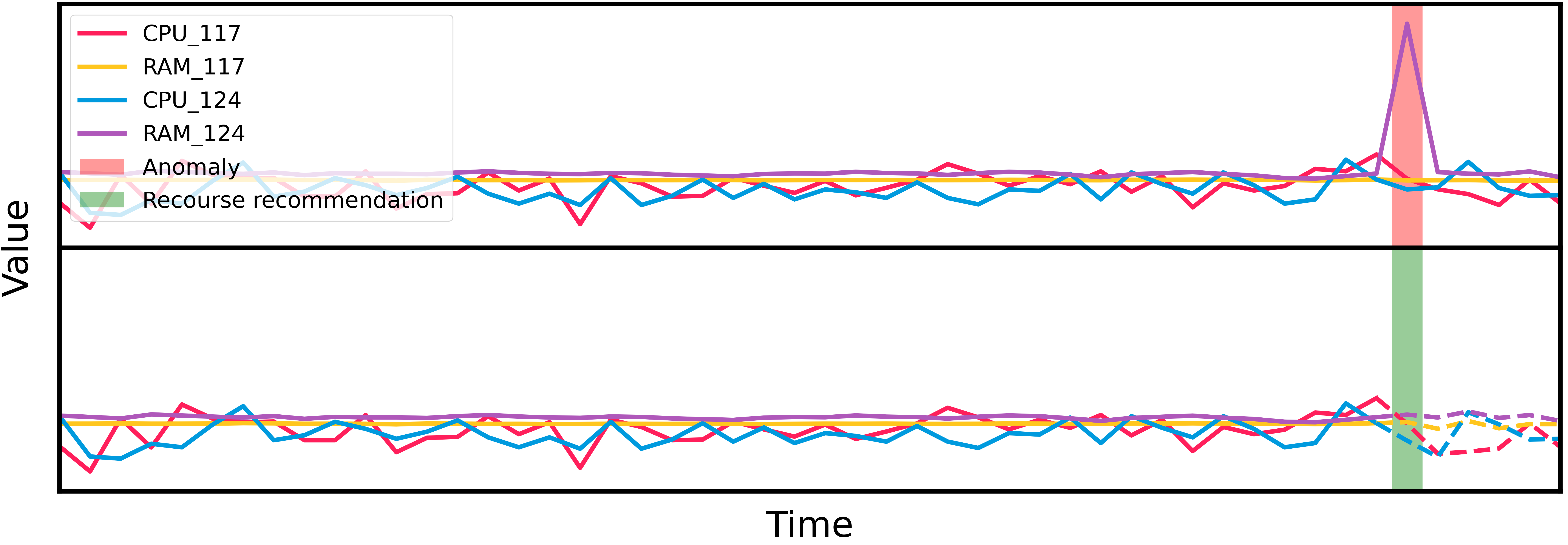
Figure 1. Recourse recommendations for flipping an abnormal status of a distribution system to a normal status.

In this work, we aim to recommend recourse actions to flip abnormal outcomes predicted by an anomaly detection model. The key challenge to recommending proper actions is that due to the nature of multivariate time series, any recourse actions on the current time step has a downstream impact governed by causal relationships. Therefore, the recourse actions in an abnormal time step should not only fix the current step but also ensure the normality in the following time steps.

We propose a framework for algorithmic Recourse in time series Anomaly Detection (RecAD), which is able to recommend recourse actions to flip the abnormal outcome. We first leverage UnSupervised Anomaly Detection for multivariate time series (USAD) (Audibert et al., 2020) as the base anomaly detection model, which detects the abnormal time step based on the reconstruction error of an autoencoder model. Once an abnormal time step is detected, RecAD can predict recourse actions to flip the abnormal outcomes by minimizing the reconstruction error of the abnormal time step. More importantly, due to the interdependence of multivariate time series, the recourse actions on the abnormal time step have downstream impacts and make the following time series unobservable in the counterfactual world. To quantify the downstream impact, RecAD derives the counterfactual time series after recourse based on the Abduction-Action-Prediction process (Pearl, 2009) governed by the causal relationships in the multivariate time series. Then, the training objective of RecAD is to ensure after applying the recourse actions, the current and the downstream counterfactual time series are predicted as normal.

The contribution of this paper can be summarized as follows. 1) We propose a novel framework for algorithmic recourse in time series anomaly detection, called RecAD. To the best of our knowledge, this is the first work on this topic. 2) RecAD considers the downstream impact of the intervention on the abnormal time step by deriving the counterfactual time series after the intervention. The goal is to ensure the following time series after intervention should also be normal. 3) The empirical studies on two synthetic and one real-world datasets show the effectiveness of RecAD for recommending recourse in time series anomaly detection.

2. Related Work

2.1. Time Series Anomaly Detection

A time series anomaly is defined as a sequence of data points that deviates from frequent patterns in the time series (Schmidl et al., 2022). Recently, a large number of deep learning-based approaches have been developed for time series anomaly detection (Schmidl et al., 2022; Blázquez-García et al., 2021). Most of the approaches are trained in the semi-supervised setting, which assumes the availability of normal time series. Then, in the test phase, the anomaly detection model can mark anomalies that are different from normal behavior measured by an anomaly score. In this work, given a detected abnormal time series, we would further like to recommend recourse actions to flip the abnormal outcome.

2.2. Algorithmic Recourse

Algorithmic recourse is to provide explanations and recommendations to flip unfavorable outcomes by an automated decision-making system (Karimi et al., 2022). Specifically, given a predictive model and a sample having an unfavorable prediction from the model, algorithmic recourse is to identify the minimal consequential recommendation that leads to a favorable prediction from the model. The key challenge of identifying the minimal consequential recommendation is to consider the causal relationships governing the data. Any recommended actions on a sample should be carried out via structural interventions leading to a counterfactual instance. Multiple algorithmic recourse algorithms on binary classification models have developed (Karimi et al., 2020, 2021; von Kügelgen et al., 2022; Dominguez-Olmedo et al., 2022). Recently, algorithmic recourse for anomaly detection on tabular data is also discussed (Datta et al., 2022). However, the existing study also does not consider causal relationships when generating counterfactuals. In this work, we focus on addressing the algorithmic recourse for anomaly detection in multivariate time series with the consideration of causal relationships.

3. Preliminary

3.1. Granger Causality

Granger causality (Granger, 1969; Dahlhaus and Eichler, 2003) is commonly used for modeling causal relationships in multivariate time series. The key assumption is that if the prediction of the future value $Y$ can be improved by knowing past elements of $X$, then $X$ “Granger causes” $Y$. Let a stationary time-series as $\mathcal{X}=(\mathbf{x}_{1},\dots,\mathbf{x}_{t},\dots,\mathbf{x}_{T})$, where $\mathbf{x}_{t}\in\mathbb{R}^{d}$ is a d-dimensional vector (e.g., d-dimensional time series data from $d$ sensors) at a specific time $t$. Suppose that the true data generation mechanism is defined in the form of

(1) $$x_{t}^{(j)}\mathrel{\mathop{\mathchar 58\relax}}=f^{(j)}(\mathbf{x}^{(1)}_{\leq t-1},\cdots,\mathbf{x}^{(d)}_{\leq t-1})+u^{(j)}_{t},\text{ for }1\leq j\leq d,$$

where $\mathbf{x}_{\leq t-1}^{(j)}=[\cdots,x_{t-2}^{(j)},x_{t-1}^{(j)}]$ denotes the present and past of series $j$; $u^{(j)}_{t}$ indicates exogenous variable of time series $j$ at time step $t$; $\mathcal{F}=\{f^{(1)},...,f^{(d)}\}$ is a set of nonlinear functions, and $f^{(j)}(\cdot)\in\mathcal{F}$ is a nonlinear function for time series $j$ that captures how the past values impact the future values of $\mathbf{x}^{(j)}$. Then, the time series $i$ Granger causes $j$, if $f^{(j)}$ depends on $\mathbf{x}_{\leq t-1}^{(i)}$, i.e., $\exists{\mathbf{x}^{\prime}}_{\leq t-1}^{(i)}\neq\mathbf{x}_{\leq t-1}^{(i)}\mathrel{\mathop{\mathchar 58\relax}}f^{(j)}(\mathbf{x}^{(1)}_{\leq t-1},\cdots,{\mathbf{x}^{\prime}}_{\leq t-1}^{(i)},\cdots,\mathbf{x}^{(d)}_{\leq t-1})$ $\neq f^{(j)}(\mathbf{x}^{(1)}_{\leq t-1},\cdots,\mathbf{x}_{\leq t-1}^{(i)},\cdots,\mathbf{x}^{(d)}_{\leq t-1})$.

3.2. Generalised Vector Autoregression (GVAR)

Granger causal inference has been extensively studied (Nauta et al., 2019; Tank et al., 2021; Marcinkevičs and Vogt, 2021; Lütkepohl, 2005). Recently, a generalized vector autoregression (GVAR) is developed to model nonlinear Granger causality in time series by leveraging neural networks (Marcinkevičs and Vogt, 2021). GVAR models the Granger causality of the $t$-th time step given the past $K$ lags by

(2) $$\mathbf{x}_{t}=\sum_{k=1}^{K}g_{k}(\mathbf{x}_{t-k})\mathbf{x}_{t-k}+\mathbf{u}_{t},$$

where $g_{k}(\cdot)\mathrel{\mathop{\mathchar 58\relax}}\mathbb{R}^{d}\rightarrow\mathbb{R}^{d\times d}$ is a feedforward neural network predicting a coefficient matrix at time step $t-k$; $\mathbf{u}_{t}$ is the exogenous variable for time step $t$. The element $(i,j)$ of the coefficient matrix from $g_{k}(\mathbf{x}_{t-k})$ indicates the influence of $x^{(j)}_{t-k}$ on $x^{(i)}_{t}$. Meanwhile, $K$ neural networks are used to predict $\mathbf{x}_{t}$. Therefore, relationships between $d$ variables over $K$ time lags can be explored by inspecting $K$ coefficient matrices. The $K$ neural networks are trained by the objective function: $\mathcal{L}=\frac{1}{T-K}\sum_{t=K+1}^{T}\|\mathbf{x}_{t}-\hat{\mathbf{x}}_{t}\|_{2}+\frac{\lambda}{T-K}\sum_{t=K+1}^{T}R(\mathcal{M}_{t})+\frac{\gamma}{T-K-1}\sum_{t=K+1}^{T-1}\|\mathcal{M}_{t+1}-\mathcal{M}_{t}\|_{2}$, where $\hat{\mathbf{x}}_{t}=\sum_{k=1}^{K}g_{k}(\mathbf{x}_{t-k})\mathbf{x}_{t-k}$ indicates the predicted value GVAR; $\mathcal{M}_{t}\mathrel{\mathop{\mathchar 58\relax}}=[g_{K}(\mathbf{x}_{t-K})\mathrel{\mathop{\mathchar 58\relax}}g_{K-1}(\mathbf{x}_{t-K+1})\mathrel{\mathop{\mathchar 58\relax}}\cdots\mathrel{\mathop{\mathchar 58\relax}}g_{1}(\mathbf{x}_{t-1})]$ indicates the concatenation of generalized coefficient matrices over the past the $K$ time steps; $R(\cdot)$ is the penalty term for sparsity, such as L1 or L2 norm; the third term is a smooothness penalty; $\lambda$ and $\gamma$ are hyperparameters. After training, the generalized coefficient predicted by $g_{k}(\mathbf{x}_{t-k})$ indicates the causal relationships between time series at the time lag $k$.

4. Framework

In this work, we aim to achieve algorithmic recourse for anomaly detection in multivariate time series. To this end, UnSupervised Anomaly Detection for multivariate time series (USAD) (Audibert et al., 2020) is adopted as a base anomaly detection model. After detecting the abnormal time steps, we propose to recommend recourse actions to flip the abnormal outcome, where the action values can fix the abnormal behavior with the minimum cost. Because the variables in a time series have causal connections through time, when recommending actions, we should consider the downstream impact on other variables. Therefore, we develop a framework for algorithmic Recourse in time series Anomaly Detection (RecAD), which is able to predict the recourse actions that fix the abnormal time series.

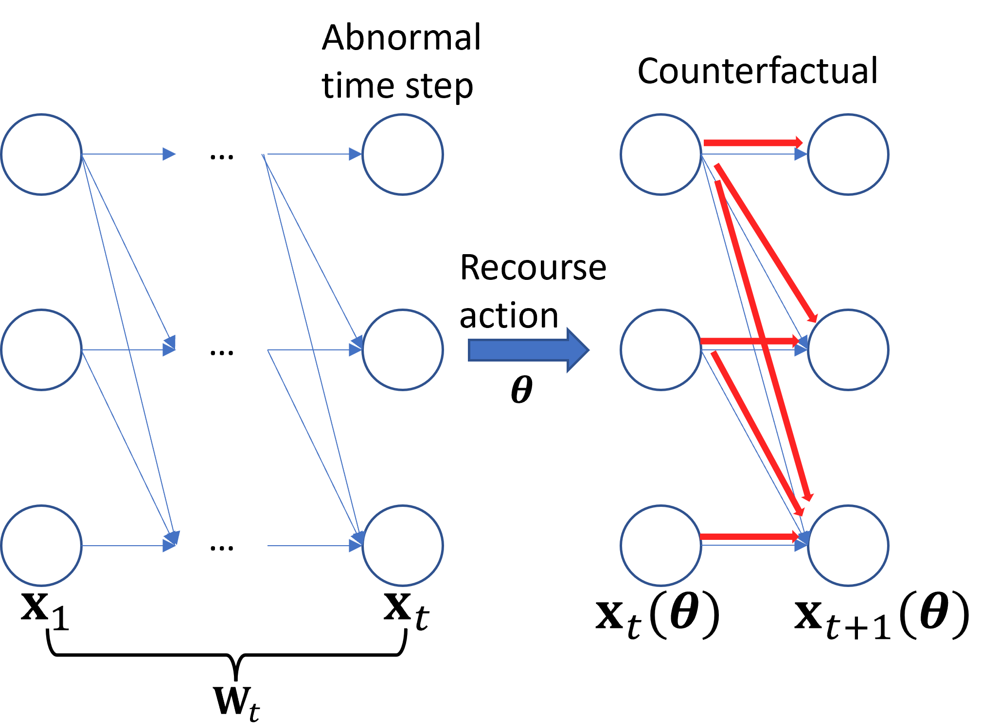
Figure 2. Algorithmic Recourse on Multivariate Time Series

Anomaly in multivariate time series. Based on the structural equation of multivariate time series, we propose to describe the anomaly from the perspective of causal relationships in multivariate time series:

(3) $$x_{t}^{(j)}\mathrel{\mathop{\mathchar 58\relax}}=f^{(j)}(\mathbf{x}^{(1)}_{\leq t-1},\cdots,\mathbf{x}^{(d)}_{\leq t-1})+u^{(j)}_{t}+\epsilon^{(j)}_{t},\text{ for }1\leq j\leq d.$$

The anomaly term $\epsilon^{(j)}_{t}$ can be due to either an external intervention or a structural intervention. The external intervention (i.e., non-causal anomaly) indicates a significantly deviating value in its exogenous variable $\tilde{u}^{(j)}_{t}$ and can be defined as: $x_{t}^{(j)}=f^{(j)}(\mathbf{x}^{(1)}_{\leq t-1},\cdots,\mathbf{x}^{(d)}_{\leq t-1})+\tilde{u}^{(j)}_{t}=f^{(j)}(\mathbf{x}^{(1)}_{\leq t-1},\cdots,\mathbf{x}^{(d)}_{\leq t-1})+u^{(j)}_{t}+\epsilon^{(j)}_{t},\text{ for }1\leq j\leq d$, where $\tilde{u}^{(j)}_{t}=u^{(j)}_{t}+\epsilon^{(j)}_{t}$. The structural intervention (i.e., causal anomaly) indicates the replacement of the structural functions $\mathcal{F}$ with abnormal functions $\tilde{\mathcal{F}}$ and can be defined as: $x_{t}^{(j)}=\tilde{f}^{(j)}(\mathbf{x}^{(1)}_{\leq t-1},\cdots,\mathbf{x}^{(d)}_{\leq t-1})+u^{(j)}_{t}=f^{(j)}(\mathbf{x}^{(1)}_{\leq t-1},\cdots,\mathbf{x}^{(d)}_{\leq t-1})+u^{(j)}_{t}+\epsilon^{(j)}_{t},\text{ for }1\leq j\leq d$, where $\tilde{f}^{(j)}(\mathbf{x}^{(1)}_{\leq t-1},\cdots,\mathbf{x}^{(d)}_{\leq t-1})$ is an abnormal function for the time series $j$ at time $t$. The anomaly term caused by the change of causal relationships is given by $\epsilon^{(j)}_{t}=\tilde{f}^{(j)}(\mathbf{x}^{(1)}_{\leq t-1},\cdots,\mathbf{x}^{(d)}_{\leq t-1})-f^{(j)}(\mathbf{x}^{(1)}_{\leq t-1},$ $\cdots,\mathbf{x}^{(d)}_{\leq t-1})$ which is time-dependent.

Equation (3) also follows the intuitive definition of an anomaly as an observation that deviates from some concepts of normality (Ruff et al., 2021; Cook et al., 2019). Here, normality indicates the structural equation without the anomaly term $\epsilon^{(j)}_{t}$.

4.1. Problem Formulation

Denote a multivariate time series as $\mathcal{X}=(\mathbf{x}_{1},\dots,\mathbf{x}_{t},\dots,\mathbf{x}_{T})$, where each time step $\mathbf{x}_{t}\in\mathbb{R}^{d}$ indicates an observation measured at time step $t$. Following the common setting for time series anomaly detection (Audibert et al., 2020; Tuli et al., 2022), given a time series $\mathcal{X}$, to model the local dependence between a time step $\mathbf{x}_{t}$ and past lags, we first define a local window with length $K$ as $\mathbf{W}_{t}=(\mathbf{x}_{t-K+1},...,\mathbf{x}_{t})$ and convert a time series $\mathcal{X}$ to a sequence of sliding windows $\mathcal{W}=(\mathbf{W}_{K},\mathbf{W}_{K+1},...,\mathbf{W}_{T})$. The multivariate time series anomaly detection approaches aim to label whether a time step $\mathbf{x}_{t}$ is abnormal based on a score function $s(\cdot)$ given the time window $\mathbf{W}_{t}$. If $s(\mathbf{W}_{t})>\tau$, then the last time step $\mathbf{x}_{t}$ will be labeled as abnormal.

When a sliding window $\mathbf{W}_{t}$ is detected as abnormal, we would like to recommend recourse actions $\bm{\theta}_{t}$ on the actionable variables at the time step $\mathbf{x}_{t}$ to reverse the abnormal outcome. Meanwhile, as the time steps keep coming in, if the following sliding window is still abnormal, we would keep recommending recourse actions until the time series is normal.

As shown in Figure 2, in the training phase, once we intervene in a time step $\mathbf{x}_{t}$, the following time series is in the counterfactual world as the intervention has the downstream impact, which is unobservable. To properly train the model for action recommendations, the key is to derive the counterfactual time series, denoted as $\mathbf{W}^{CF}_{t+1}=(\mathbf{x}_{2},...,\mathbf{x}_{t}+\bm{\theta}_{t},\mathbf{x}_{t+1}(\bm{\theta}_{t}))$, where $\mathbf{x}_{t+1}(\bm{\theta}_{t})$ indicates the counterfactual time step $t+1$ after conducting intervention on $\mathbf{x}_{t}$. If $\mathbf{W}^{CF}_{t+1}$ is still detected as abnormal, further recourse actions will be recommended on the counterfactual data $\mathbf{x}_{t+1}(\bm{\theta}_{t})$.

4.2. Anomaly Detection for Time Series

In this work, we adopt UnSupervised Anomaly Detection for multivariate time series (USAD) (Audibert et al., 2020) which is a state-of-the-art autoencoder-based anomaly detection model. USAD consists of two autoencoders, i.e., $AE_{1}$ and $AE_{2}$, with a shared encoder and two independent decoders, and derives the anomaly score function $s(\cdot)$ based on the reconstruction errors of two autoencoders. In the training phase, given a set of normal sliding windows, USAD combines traditional reconstruction-based training with adversarial training to capture the normal patterns of time series. Specifically, reconstruction-based training will let both autoencoders learn how to reproduce the input window $\mathbf{W}$, i.e., $\mathcal{L}_{AE_{*}}=\|\mathbf{W}-AE_{*}(\mathbf{W})\|_{2}$, where $AE_{*}$ indicates either $AE_{1}$ or $AE_{2}$. The goal of adversarial training is for $AE_{1}$ to deceive $AE_{2}$, while $AE_{2}$ learns to distinguish between real data and reconstructed data from $AE_{1}$, i.e., $\mathcal{L}_{AD}=\underset{AE_{1}}{\text{min}}\>\underset{AE_{2}}{\text{max}}\|\mathbf{W}-AE_{2}(AE_{1}(\mathbf{W}))\|_{2}$.

After training, the anomaly score of a new window $\mathbf{W}^{*}$ is then calculated using the combination of reconstruction errors of two autoencoders,

(4) $$s(\mathbf{W}^{*})\!=\!\alpha\|\mathbf{W}-AE_{1}(\mathbf{W}^{*})\|_{2}\!+\!\beta\|\mathbf{W}^{*}\!-\!AE_{2}(AE_{1}(\mathbf{W}^{*}))\|_{2},$$

where $\alpha$ and $\beta$ are hyperparameters.

4.3. Algorithmic Recourse

When a sliding window $\mathbf{W}_{t}$ is detected as abnormal, we then recommend recourse actions on $\mathbf{x}_{t}$ with the consideration of downstream impacts.

4.3.1. Recourse on the abnormal time step

Given an abnormal point $\mathbf{x}_{t}$ and the previous $K-1$ time lags in $\mathbf{W}_{t}=(\mathbf{x}_{t-K+1},\dots,\mathbf{x}_{t-1},\mathbf{x}_{t})$, we formulate the recourse on $\mathbf{x}_{t}$ as soft intervention,

(5) $$\mathbf{x}_{t}(\bm{\theta}_{t})=\mathbf{x}_{t}+\bm{\theta}_{t},$$

where $\bm{\theta}_{t}$ is the action values on $\mathbf{x}_{t}$ derived by a function, i.e., $\bm{\theta}_{t}=h_{\phi}(\cdot)$ parameterized by $\phi$.

In order to successfully flip the abnormal outcomes, we consider two types of information for recourse prediction via $h_{\phi}(\cdot)$, time lag exclusion term $\Delta_{t}$ and the past window $\mathbf{W}_{t-1}$. As shown in Equation (3), the anomaly in multivariate time series is due to an additional anomaly term. Therefore, we derive the time lag independent term $\Delta_{t}$ at time $t$ as $\Delta_{t}=\mathbf{x}_{t}-\hat{\mathbf{x}}_{t}$, where $\hat{\mathbf{x}}_{t}$ is the expected values given $\mathbf{W}_{t-1}$ derived by GVAR. As GVAR can simulate the nonlinear multivariate GC functions $\mathcal{F}$, $\Delta_{t}$ contains only independent noise term and anomaly term at time $t$.

Let $\bm{\theta}_{t}=h_{\phi}(\mathbf{W}_{t-1},\Delta_{t})$ be the function for predicting the recourse action given the previous $K$ time lags $\mathbf{W}_{t-1}$ and $\Delta_{t}$ at time step $t$ parameterized by $\phi$, which is defined below:

(6) $$\begin{split}\mathbf{z}_{t-1}&=LSTM(\mathbf{W}_{t-1})\quad\mathbf{z}_{\Delta}=FFNN(\Delta_{t})\quad\\ \bm{\theta}_{t}&=FFNN(\mathbf{z}_{t-1}\oplus\mathbf{z}_{\Delta}),\end{split}$$

where $LSTM(\cdot)$ is the long short-term memory (LSTM) neural network; $FFNN(\cdot)$ is a feedforward neural network; and $\oplus$ indicates the vector concatenation operation. In a nutshell, to predict the recourse action, first, we adopt LSTM that takes the past $K$ time lags $\mathbf{W}_{t-1}$ as input and derives a hidden representation $\mathbf{z}_{t-1}$ of the last time step to represent $\mathbf{W}_{t-1}$. Similarly, we adopt a feedforward neural network that takes $\Delta_{t}$ as input to derive the hidden representation $\mathbf{z}_{\Delta}$. Finally, we use another feedforward neural network for recourse prediction by concatenating $\mathbf{z}_{t-1}$ and $\mathbf{z}_{\Delta}$ as input.

By applying the action $\bm{\theta}_{t}$ on $\mathbf{x}_{t}$, the counterfactual time step can be computed as $\mathbf{x}_{t}(\bm{\theta}_{t})=\mathbf{x}_{t}+\bm{\theta}_{t}$. The counterfactual window $\mathbf{W}_{t}(\bm{\theta}_{t})$ is derived by replacing $\mathbf{x}_{t}$ with $\mathbf{x}_{t}(\bm{\theta}_{t})$ in $\mathbf{W}_{t}$. To train the recourse prediction functions, the objective function is defined as:

(7) $$\mathcal{L}_{t}(\phi)=\max\left\{s(\mathbf{W}_{t}(\bm{\theta}_{t}))-\alpha\tau,0\right\}+\lambda\|\mathbf{c}\cdot\bm{\theta}_{t}\|_{2},$$

where $s(\mathbf{W}_{t}(\bm{\theta}_{t}))$ indicates the anomaly score defined in Equation (4); $\lambda$ is a hyperparameter balancing the action values on the anomaly and the flipping of abnormal outcome, $\alpha$ is another hyperparameter controlling how close the anomaly score of the counterfactual sample should be to the threshold $\tau$, $\mathbf{c}\in\mathbb{R}^{d}$ is a hyperparameter, describing the costs of revising time series (cost vector). Because in USAD, the anomaly is labeled due to a large reconstruction error on the input sample, the first term in the objective function is to ensure the counterfactual variant has a small reconstruction error. The second term, as a regularization term, ensures the minimum action cost on the original values.

Inferring the downstream impact. Based on the assumption of Granger causality, the recourse on $\mathbf{x}_{t}$ leads to the counterfactual variants of the following time steps $\mathbf{x}_{t^{\prime}}(\bm{\theta}_{t})$, where $t^{\prime}\geq t$.

To evaluate the impact of the intervention, assuming that $\mathbf{x}_{t}(\bm{\theta}_{t}),\mathbf{x}_{t+1}(\bm{\theta}_{t}),\allowbreak\dots,\mathbf{x}_{t^{\prime}}(\bm{\theta}_{t})$ is known, where $t^{\prime}\geq t$, we further derive the counterfactual quantity of the next step $\mathbf{x}_{t^{\prime}+1}$ by the Abduction-Action-Prediction (AAP) process (Pearl, 2009): 1) Abduction: update the probability $P(u^{(i)}_{t^{\prime}+1})$ to obtain $P(u^{(i)}_{t^{\prime}+1}|e)$, where $u$ indicates the exogenous variables and $e$ indicates propositional evidence; 2) Action: variables are intervened to reflect the counterfactual assumption; 3) Prediction: counterfactual reasoning occurs over the new model using updated knowledge.

Formally, based on the causal relationships learned by GVAR, the Abduction-Action-Prediction process to compute the counterfactual value in the $t^{\prime}+1$-th time step can be described below.

Step 1 (abduction):

(8) $$\mathbf{u}_{t^{\prime}+1}=\mathbf{x}_{t^{\prime}+1}-\sum_{k=1}^{K}g_{k}(\mathbf{x}_{t^{\prime}+1-k})\mathbf{x}_{t^{\prime}+1-k}$$

Step 2 (action):

(9) $$\mathbf{a}_{t^{\prime}}=\mathbf{x}_{t^{\prime}}+\bm{\theta}_{t}\text{ if }t^{\prime}=t\quad\mathbf{a}_{t^{\prime}}=\mathbf{x}_{t^{\prime}}(\bm{\theta}_{t})\text{ if }t^{\prime}>t$$

Step 3 (prediction):

(10) $$\mathbf{x}_{t^{\prime}+1}(\!\bm{\theta}_{t}\!)\!\!=\!\!\!\sum_{k=2}^{K}g_{k}(\mathbf{x}_{t^{\prime}\!+\!1\!-\!k}(\!\bm{\theta}_{t}\!))\mathbf{x}_{t^{\prime}\!+\!1\!-\!k}(\!\bm{\theta}_{t}\!)\!+\!g_{1}(\!\mathbf{a}_{t^{\prime}}\!)\mathbf{a}_{t^{\prime}}\!+\!\mathbf{u}_{t^{\prime}+1}.$$

Equations (8)-(10) provide the recursive equations for computing the counterfactual time series for $L$ ($L<K$) steps based on the AAP process. The closed form formula for computing counterfactual value $\mathbf{x}_{t+L}(\bm{\theta}_{t})$ can be derived as.

(11) $$\begin{split}\mathbf{x}_{t+L}(\bm{\theta}_{t})&=\sum_{l=0}^{L-1}g_{L-l}(\mathbf{x}_{t+l}(\bm{\theta}_{t}))\mathbf{x}_{t+l}(\bm{\theta}_{t})\\ &+\sum_{n=1+L}^{K}g_{n}(\mathbf{x}_{t+L-n})\mathbf{x}_{t+L-n}+\mathbf{u}_{t+L},\end{split}$$

where $\mathbf{u}_{t+L}$ can be derived similar to Equation (8).

Because the intervention on the $t$-th step has the downstream impact, besides ensuring the counterfactual window $\mathbf{W}_{t}(\bm{\theta}_{t})$ be normal, we would like to make sure that the following $L$ steps are also normal. Therefore, we update the objective function in Equation (7) by considering the normality of following $L$ steps,

(12) $$\mathcal{L}(\phi)\!\!=\!\!\sum_{t^{\prime}=t}^{t+L}\max\left\{s(\mathbf{W}_{t^{\prime}}(\bm{\theta}_{t}))\!\!-\!\!\alpha\tau,0\right\}\!\!+\!\!\lambda\|\mathbf{c}\cdot\bm{\theta}_{t}\|_{2}.$$

Extend to multiple recourse predictions over time series. In practice, a time series could have multiple abnormal time steps, so the algorithmic recourse algorithm should be able to keep flipping abnormal behavior. However, the challenge during the training phase is that we only observe a sequence of time series with abnormal time steps, but after conducting intervention at a time step $t$, the following time series in the counterfactual world $\mathcal{X}^{CF}$ is unobservable. Therefore, during the training phase, we need to derive the counterfactual time step, denoted as $\mathbf{x}_{t+1}^{CF}$, based on the AAP process. Then, if the counterfactual window $\mathbf{W}^{CF}_{t+1}$ is still detected as abnormal, i.e., $s(\mathbf{W}^{CF}_{t+1})>\tau$, meaning that $\mathbf{x}_{t+1}^{CF}$ is still abnormal. We would further train the model $h_{\phi}(\cdot)$ to recommend recourse actions $\theta_{t+1}$ to flip $\mathbf{x}_{t+1}^{CF}$.

Algorithm 1 shows the pseudo-code of the training process for recourse predictions with multiple abnormal time steps over time series. Let $\tilde{\mathcal{X}}^{-}$ be a set of abnormal time series detected by USAD, where each abnormal time series has at least one abnormal time step. For each abnormal time series $\mathcal{X}$ in $\tilde{\mathcal{X}}^{-}$, initializing the counterfactual time series the same as the factual data (Line 1). Note that if there is no intervention conducted yet, the counterfactual time series keeps the same as the observed time series.

Suppose a recourse action is conducted before time step $t$, we first need to derive the counterfactual time series $\mathcal{X}^{CF}$ (Line 1). To this end, we first get the sliding window $\mathbf{W}_{t}$ that contains the current time step and the sliding window $\mathbf{W}_{t-1}$ that only contains the previous time steps from the observed time series (Line 1). We further get the sliding window $\mathbf{W}^{CF}_{t}$ and $\mathbf{W}^{CF}_{t-1}$ from the counterfactual time series (Line 1). Then we can compute the excepted normal values of the factual world for the current time step $t$ by GVAR according to Equation (2) (Line 1). The time lag exclusion term $\mathbf{u}_{t}$ can be derived by Equation (8) (Line 1). Similarly, we further compute the excepted normal values of the counterfactual world for the current time step $t$ by GVAR (Line 1). As $\hat{\mathbf{x}}_{t}^{CF}$ only includes the effects of the previous time steps without any time lag exclusion values (i.e., noise term and anomaly term) for the current time step, the accurate counterfactual values for the current time step $t$ needs to consider the time lag exclusion term $\mathbf{u}_{t}$ (Line 1). The $\mathcal{X}^{CF}$ and $\mathbf{W}^{CF}_{t}$ values need to update each time step after a recourse action is conducted (Line 1).

If the updated sliding window $\mathbf{W}^{CF}_{t}$ is still detected as an anomaly (Line 1), we need to keep predicting the recourse action (Line 1. Specifically, we first compute the action values with $h_{\phi}(\cdot)$ (Line 1). The counterfactual values of the current time step $t$ can be calculated by Equation (9) (Line 1). Then we further update the values at time step $t$ of counterfactual time series $\mathbf{x}_{t}^{CF}$ with values $\mathbf{x}_{t}(\theta_{t})$, meaning that another recourse action is conducted (Line 1).

During the training phase, we expect $h_{\phi}(\cdot)$ can recommend the recourse action with the consideration of its downstream impact on future time steps. Therefore, we compute the counterfactual values for the following $L$ steps according to Equation (11) (Line 1). Then, we update the parameters in $h_{\phi}(\cdot)$ based on the objective function defined in Equation (12).

Input : Pretrained GVAR $g_{k}(\cdot)$, pretrained anomaly detector $s(\cdot)$, anomaly set $\tilde{\mathcal{X}}^{-}$

Output : $h_{\phi}(\cdot)$ for action prediction

1 foreach $\mathcal{X}\in\tilde{\mathcal{X}}^{-}$ do

2       $t\leftarrow K;\;\mathcal{X}^{CF}\leftarrow\mathcal{X};\;T\leftarrow\text{length of}\;\mathcal{X}$

3       while $t\leq T$ do

4             $\mathcal{X}^{CF},\;\mathbf{W}^{CF}_{t},\;\mathbf{W}_{t}\leftarrow\text{Counterfactual\_Generation}(\mathcal{X},\;\mathcal{X}^{CF},\;g_{k}(\cdot))$

5             if $s(\mathbf{W}^{CF}_{t})>\tau$  then

6                   $\mathbf{x}_{t}(\theta_{t}),\;h_{\phi}(\cdot)\leftarrow\text{Action\_Prediction}(\mathbf{W}_{t},\;\mathbf{W}^{CF}_{t},\;g_{k}(\cdot),\;h_{\phi}(\cdot))$

7                   Update $\mathbf{x}_{t}^{CF}$ with $\mathbf{x}_{t}(\theta_{t})$

8                   Update $\mathcal{X}^{CF}\;\text{with}\;\mathbf{x}_{t}^{CF}$

9                   Compute $\mathbf{x}_{t+1+L}(\theta_{t})$ with Eq. (11)

10                   Compute $\mathcal{L}(\phi)$ according to Eq. (12)

11                   Update $\phi=\phi-\eta\frac{\partial\mathcal{L}(\phi)}{\partial\phi}$

12            $t$ ++

13      

14Return $h_{\phi}(\cdot)$

15

16 Function Counterfactual_Generation($\mathcal{X},\;\mathcal{X}^{CF},\;g_{k}(\cdot)$):

17       Get $\mathbf{W}_{t}\;\text{from}\;\mathcal{X},\;\mathbf{W}_{t-1}=\mathbf{W}_{t}\setminus\{\mathbf{x}_{t}\}$

18       Get $\mathbf{W}^{CF}_{t}\;\text{from}\;\mathcal{X}^{CF},\;\mathbf{W}^{CF}_{t-1}=\mathbf{W}^{CF}_{t}\setminus\{\mathbf{x}_{t}^{CF}\}$

19       Compute $\hat{\mathbf{x}}_{t}=\sum_{k=1}^{K-1}g_{k}(\mathbf{x}_{t-k})\mathbf{x}_{t-k}\;\text{with}\;\mathbf{W}_{t-1}$

       Compute $\mathbf{u}_{t}=\mathbf{x}_{t}-\hat{\mathbf{x}_{t}}$

        $\triangleright$ Abduction

20       Compute $\hat{\mathbf{x}}_{t}^{CF}=\sum_{k=1}^{K-1}g_{k}(\mathbf{x}_{t-k}^{CF})\mathbf{x}_{t-k}^{CF}\;\text{with}\;\mathbf{W}_{t-1}^{CF}$

       $\mathbf{x}_{t}^{CF}=\hat{\mathbf{x}}_{t}^{CF}+\mathbf{u}_{t}$

        $\triangleright$ Prediction

21       Update $\mathcal{X}^{CF}\;\text{and}\;\mathbf{W}^{CF}_{t}\;\text{with}\;\hat{\mathbf{x}}_{t}^{CF}$

22       Return $\mathcal{X}^{CF},\;\mathbf{W}^{CF}_{t},\;\mathbf{W}_{t}$

23      

24

25 Function Action_Prediction($\mathbf{W}_{t},\;\mathbf{W}^{CF}_{t},\;g_{k}(\cdot),\;h_{\phi}(\cdot)$):

26       $\mathbf{W}_{t-1}\leftarrow\mathbf{W}_{t}\setminus\{\mathbf{x}_{t}\}$; $\mathbf{W}^{CF}_{t-1}\leftarrow\mathbf{W}^{CF}_{t}\setminus\{\mathbf{x}_{t}^{CF}\}$

27       Compute $\hat{\mathbf{x}}_{t}=\sum_{k=1}^{K-1}g_{k}(\mathbf{x}_{t-k})\mathbf{x}_{t-k}\;\text{with}\;\mathbf{W}_{t-1}$

28       Compute $\Delta_{t}=\mathbf{x}_{t}-\hat{\mathbf{x}}_{t}$

29       Compute $\bm{\theta}_{t}=h_{\phi}(\mathbf{W}_{t-1}^{CF},\Delta_{t})$

       $\mathbf{x}_{t}(\theta_{t})=\mathbf{x}_{t}^{CF}+\bm{\theta}_{t}$

        $\triangleright$ Action

30       Return $\mathbf{x}_{t}(\theta_{t}),\;h_{\phi}(\cdot)$

Algorithm 1 Training Procedure of RecAD

4.3.2. Recourse prediction in the test phase

After completing the training process, the recourse prediction function $h_{\phi}(\cdot)$ is capable of predicting the appropriate recourse recommendations for each detected anomaly. In the test phase, the multivariate time series is considered as streaming data that is continuously fed into our framework. USAD starts by analyzing the first $K$ time steps to detect any anomalies. If an anomaly is detected with the $K$ time step, RecAD will utilize the information gathered up to that point $\mathbf{W}_{K-1}$ to make a recourse recommendation for the last time step $\mathbf{x}_{K}$. Then, different from the training phase, where we can only derive the counterfactual time series after intervention based on the AAP process, as the time series comes in as a stream, we can directly observe the following time series after the intervention. We will continue monitoring the incoming data to detect any anomalies and further recommend recourse actions once an abnormal time step is detected. This process will continue as long as the system is receiving input data.

5. Experiments

5.1. Experimental Setups

5.1.1. Datasets

We conduct experiments on two semi-synthetic datasets and one real-world dataset. The purposes of using semi-synthetic datasets are as follows. 1) We can derive the ground truth downstream time series after the intervention on the abnormal time step based on the data generation equations in the test phase. 2) We can evaluate the fine-grained performance of RecAD by injecting different types of anomalies.

Linear Dataset (Marcinkevičs and Vogt, 2021) is a synthetic time series dataset with linear interaction dynamics. We adopt the structural equations defined in (Marcinkevičs and Vogt, 2021) that are

defined as:

(13) $$x^{(1)}_{t} =a_{1}x^{(1)}_{t-1}+u^{(1)}_{t}+\epsilon^{(1)}_{t},$$

$$x^{(2)}_{t} =a_{2}x^{(2)}_{t-1}+a_{3}x^{(1)}_{t-1}+u^{(2)}_{t}+\epsilon^{(2)}_{t},$$

$$x^{(3)}_{t} =a_{4}x^{(3)}_{t-1}+a_{5}x^{(2)}_{t-1}+u^{(3)}_{t}+\epsilon^{(3)}_{t},$$

$$x^{(4)}_{t} =a_{6}x^{(4)}_{t-1}+a_{7}x^{(2)}_{t-1}+a_{8}x^{(3)}_{t-1}+u^{(4)}_{t}+\epsilon^{(4)}_{t},$$

where coefficients $a_{i}\sim\mathcal{U}([-0.8,-0.2]\cup[0.2,0.8])$, additive innovation terms $u^{(\cdot)}_{t}\sim\mathcal{N}(0,0.16)$, and anomaly term $\epsilon^{(\cdot)}_{t}$.

Abnormal behavior injection. For non-causal point anomalies, the anomaly term is single or multiple extreme values for randomly selected time series variables at a specific time step $t$. For example, a point anomaly at time step $t$ can be generated with an abnormal term $\bm{\epsilon}_{t}=[0,2,4,0]$, which means the second and third time series have extreme values.

For non-causal sequence anomalies, the anomaly terms are function-generated values in a given time range. For instance, setting $\epsilon^{(1)}_{t+i}=0.1\times i,\;\text{for}\;0\leq i\leq n$, will cause a trend anomaly for time series variable $x^{(1)}$; setting $\epsilon^{(1)}_{t+i}\sim\mathcal{N}(0,0.16),\;\text{for}\;0\leq i\leq n$, will cause a shapelet anomaly; and setting $\epsilon^{(1)}_{t+i}=(a_{1}x^{(1)}_{t+2i-1}+u^{(1)}_{t+2i})+(a_{1}x^{(1)}_{t+2i-2}+u^{(1)}_{t+2i-1})-(a_{1}x^{(1)}_{t+i-1}+u^{(1)}_{t+i}),\;\text{for}\;0\leq i\leq n$, will cause a seasonal anomaly.

For causal sequence anomalies, we consider two scenarios: 1) changing the coefficients $\mathcal{A}=\{a_{1},a_{2},\cdots,a_{8}\}$ from a normal one to a different one in a time range $t$ to $t+n$; 2) changing generative functions from the original equation to the following equation:

(14) $$x^{(1)}_{t} =a_{1}x^{(1)}_{t-1}+a_{2}x^{(3)}_{t-1}+a_{3}x^{(4)}_{t-1}+u^{(1)}_{t}+\epsilon^{(1)}_{t},$$

$$x^{(2)}_{t} =a_{4}x^{(2)}_{t-1}+a_{5}x^{(1)}_{t-1}+u^{(2)}_{t}+\epsilon^{(2)}_{t},$$

$$x^{(3)}_{t} =a_{6}x^{(3)}_{t-1}+u^{(3)}_{t}+\epsilon^{(3)}_{t},$$

$$x^{(4)}_{t} =a_{7}x^{(4)}_{t-1}+u^{(4)}_{t}+\epsilon^{(4)}_{t}.$$

Lotka-Volterra (Bacaër, 2011) is another synthetic time series model that simulates a prairie ecosystem with multiple species. We follow the structure from (Marcinkevičs and Vogt, 2021), which defines as:

(15) $$\frac{d\mathbf{x}^{(i)}}{dt} =\alpha\mathbf{x}^{(i)}-\beta\sum_{j\in Pa(\mathbf{x}^{(i)})}\mathbf{y}^{(j)}-\eta(\mathbf{x}^{(i)})^{2},\;\text{for}\;1\leq j\leq p,$$

$$\frac{d\mathbf{y}^{(j)}}{dt} =\delta\mathbf{y}^{(j)}\sum_{k\in Pa(\mathbf{y}^{(j)})}\mathbf{x}^{(k)}-\rho\mathbf{y}^{(j)},\;\text{for}\;1\leq j\leq p,$$

$$x^{(i)}_{t} =x^{(i)}_{t}+\epsilon^{(i)}_{t},\;\text{for}\;1\leq j\leq p,$$

$$y^{(j)}_{t} =y^{(j)}_{t}+\epsilon^{(j)}_{t},\;\text{for}\;1\leq j\leq p,$$

where $\mathbf{x}^{(i)}$ and $\mathbf{y}^{(j)}$ denote the population sizes of prey and predator, respectively; $\alpha,\beta,\eta,\delta,\rho$ are parameters that decide the strengths of interactions, $Pa(\mathbf{x}^{(i)})$ and $Pa(\mathbf{y}^{(j)})$ correspond the Granger Causality between prey and predators for $\mathbf{x}^{(i)}$ and $\mathbf{y}^{(j)}$ respectively, and $\epsilon^{(\cdot)}_{t}$ is the abnormal term. We adopt 10 prey species and 10 predator species.

Abnormal behavior injection. We adopt similar strategies as used in the Linear Dataset to inject abnormal behavior.

For point anomalies and non-causal sequence anomalies, we perform a similar procedure as the linear dataset, i.e., randomly select time series variables at a specific time step $t$ and assign single or multiple extreme values as point anomalies, and assign function-generated abnormal terms for a time range from $t$ to $t+n$ as sequence anomalies.

For causal sequence anomalies, we still consider two scenarios: 1) changing the coefficients $\alpha,\beta,\eta,\delta,\rho$ to different values than the normal ones; 2) changing $Pa(\mathbf{x}^{(i)})$ and $Pa(\mathbf{y}^{(j)})$ to different ones from the original generative functions Equation (15).

Multi-Source Distributed System (MSDS) (Nedelkoski et al., 2020) is a real-world dataset that contains distributed traces, application logs, and metrics from an OpenStack testbed. MSDS consists 10-dimensional time series. The fault injections are treated as anomalies. The first half of MSDS without fault injection is used as a training set, while the second half includes 5.37% time steps as fault injections, which is used as a test set. As the real-world dataset, we cannot observe the downstream time series after the intervention. Therefore, in the test phase, we use GVAR and AAP to generate the counterfactual time series for evaluation.

Table 1. Statistics of three datasets for anomaly detection.

Dataset	Dim.	Train	Test (Anomalies %)
			Point	Non-causal Seq.	Causal Seq.
Linear	4	50,000	250,000 (2%)	250,000 (6%)	250,000 (6%)
Lotka-Volterra	20	100,000	500,000 (1%)	500,000 (3%)	500,000 (3%)
MSDS	10	146,340	146,340 (5.37%)

Table 1 shows the statistics of three datasets. Training datasets only consist of normal time series. Note that the test sets listed in Table 1 are used for evaluating the performance of anomaly detection. After detecting the abnormal time series in the test set, for the synthetic datasets, we use 50% of abnormal time series for training RecAD and another 50% for evaluating the performance of RecAD on recourse prediction, while for the MSDS dataset, we use 80% of abnormal time series for training RecAD and the rest 20% for evaluation.

5.1.2. Baselines

To our best knowledge, there is no causal algorithmic recourse approach in time series anomaly detection. We compare RecAD with the following baselines: 1) Multilayer perceptron (MLP) which is trained with the normal flattened sliding windows to predict the normal values for the next step; 2) LSTM which can capture the information over long periods of time and learn complex temporal dependencies to make predictions for the next step; 3) Vector Autoregression (VAR) is a statistical model that used to analyze GC within multivariate time series data and predict future values; 4) Generalised Vector Autoregression (GVAR) (Marcinkevičs and Vogt, 2021) is an extension of self-explaining neural network that can infer nonlinear multivariate GC and predict values of the next step.

For all the baselines, in the training phase, we train them to predict the last value in a time window on the normal time series so that they can capture the normal patterns. In the testing phase, when a time window is detected as abnormal by USAD for the first time, indicating the last time step $\mathbf{x}_{t}$ is abnormal, we use baselines to predict the expected normal value in the last time step $\tilde{\mathbf{x}}_{t}$. Then, the recourse action values can be derived as $\theta_{t}=\tilde{\mathbf{x}}_{t}-\mathbf{x}_{t}$. For the sequence anomalies, we keep using the baselines to predict the expected normal values and derive the action values by comparing them with the observed values.

5.1.3. Evaluation Metrics

We evaluate the performance of algorithmic recourse based on the following three metrics.

1) Flipping ratio, which is to show the effectiveness of algorithms for algorithmic recourse.

$$\text{Flipping Ratio}=\frac{\text{Number of flipped time steps}}{\text{All detected abnormal time steps}}$$

2) Action cost per multivariate time series, which is to check the efficiency of predicted actions.

$$\text{Action Cost}=\frac{\text{Total action cost}}{\text{\# of abnormal multivariate time series}},$$

where the “Total action cost” indicates the action cost ($\|\mathbf{c}\cdot\bm{\theta}_{t}\|_{2}$) to flip all the abnormal data in the test set.

3) Action step per multivariate time series, which is to show how many action steps are needed to flip the abnormal time series.

$$\text{Action Step}=\frac{\text{Total number of action time steps}}{\text{\# of abnormal multivariate time series}}$$

5.1.4. Implementation Details

Similar to (Audibert et al., 2020), we adopt a sliding window with sizes 5, 5, and 10 for the Linear, Lotka-Volterra, and MSDS datasets, respectively. We set the hyperparameters for GVAR by following (Marcinkevičs and Vogt, 2021). When training $h_{\phi}(\cdot)$, we set $L$ in the objective function as $L=1$, which is to ensure the following one time step should be normal. The cost vector $\mathbf{c}$ can be changed according to the requirements or prior knowledge. Because the baseline models are prediction-based models that cannot take the cost into account, to be fair, we use $\mathbf{1}$ as the cost vector. For baselines, MLP is a feed-forward neural network with a structure of ($(K-1)*d$)-100-100-100-$d$ that the input is the flattened vector of $K-1$ time steps with $d$ dimensions and the output is the predicted value of the next time step. The LSTM model consists of one hidden layer with 100 dimensions and is connected with a fully connected layer with a structure of 100-$d$. We use statsmodels to implement the VAR model. The baseline GVAR model is the same as GVAR within our framework. To implement $h_{\phi}(\cdot)$ in RecAD, we utilize an LSTM that consists of one hidden layer with 100 dimensions and a feed-forward network with structure $d$-100. Then we use another feed-forward network with a structure of 200-$d$ to predict the intervention values. Our code is available online.

5.2. Experimental Results

5.2.1. Evaluation Results on Synthetic Datasets.

We first report the experimental results with standard deviations over 10 runs on synthetic datasets as we can conduct more fine-grained evaluations on synthetic datasets.

Table 2. Anomaly detection on synthetic datasets.

Anomaly Types	Metrics	Linear	Lotka-Volterra
Non-causal Point	F1	$0.749_{\pm 0.022}$	$0.787_{\pm 0.106}$
	AUC-PR	$0.619_{\pm 0.024}$	$0.840_{\pm 0.116}$
	AUC-ROC	$0.816_{\pm 0.016}$	$0.851_{\pm 0.068}$
Non-causal Seq.	F1	$0.878_{\pm 0.011}$	$0.677_{\pm 0.061}$
	AUC-PR	$0.798_{\pm 0.015}$	$0.519_{\pm 0.026}$
	AUC-ROC	$0.914_{\pm 0.010}$	$0.794_{\pm 0.089}$
Causal Seq.	F1	$0.756_{\pm 0.003}$	$0.714_{\pm 0.020}$
	AUC-PR	$0.604_{\pm 0.004}$	$0.559_{\pm 0.016}$
	AUC-ROC	$0.877_{\pm 0.002}$	$0.824_{\pm 0.078}$

The performance of anomaly detection. We evaluate the performance of USAD for anomaly detection in terms of the F1 score, the area under the precision-recall curve (AUC-PR), and the area under the receiver operating characteristic (AUC-ROC) on two synthetic datasets. Table 2 shows the evaluation results. Overall, USAD can achieve promising performance on different types of anomalies, which lays a solid foundation for recourse prediction.

Table 3. The performance of recourse prediction on non-causal anomaly.

Model	Linear						Lotka-Volterra
	Point			Seq.			Point			Seq.
	Flipping Ratio $\uparrow$	Action Cost $\downarrow$	Action Step $\downarrow$	Flipping Ratio $\uparrow$	Action Cost $\downarrow$	Action Step $\downarrow$	Flipping Ratio $\uparrow$	Action Cost $\downarrow$	Action Step $\downarrow$	Flipping Ratio $\uparrow$	Action Cost $\downarrow$	Action Step $\downarrow$
MLP	$0.778_{\pm 0.054}$	$8.406_{\pm 0.257}$	$1.188_{\pm 0.051}$	$0.867_{\pm 0.048}$	$22.394_{\pm 0.545}$	$2.261_{\pm 0.027}$	$0.741_{\pm 0.126}$	$277.580_{\pm 117.126}$	$1.237_{\pm 0.180}$	$0.688_{\pm 0.259}$	$761.550{\pm 64.422}$	$2.195_{\pm 0.757}$
LSTM	$0.807_{\pm 0.045}$	$8.383_{\pm 0.253}$	$1.170_{\pm 0.040}$	$0.878_{\pm 0.044}$	$22.439_{\pm 0.553}$	$2.248_{\pm 0.031}$	$0.893_{\pm 0.087}$	$313.510_{\pm 124.921}$	$1.096_{\pm 0.061}$	$0.889_{\pm 0.097}$	$1590.483_{\pm 85.126}$	$1.339_{\pm 0.145}$
VAR	$0.676_{\pm 0.063}$	$8.841_{\pm 0.224}$	$1.311_{\pm 0.077}$	$0.765_{\pm 0.061}$	$23.696_{\pm 0.511}$	$2.434_{\pm 0.037}$	$0.558_{\pm 0.166}$	$326.967_{\pm 126.322}$	$1.57_{\pm 0.324}$	$0.504_{\pm 0.151}$	$1445.084_{\pm 189.943}$	$2.570_{\pm 0.676}$
GVAR	$0.775_{\pm 0.053}$	$8.446_{\pm 0.249}$	$1.207_{\pm 0.052}$	$0.848_{\pm 0.051}$	$22.415_{\pm 0.547}$	$2.287_{\pm 0.029}$	$0.493_{\pm 0.332}$	$270.335_{\pm 117.223}$	$2.020_{\pm 1.049}$	$0.606_{\pm 0.266}$	$\bf{749.792_{\pm 105.656}}$	$2.547_{\pm 0.905}$
RecAD	$\bf{0.901_{\pm 0.035}}$	$\bf{8.201_{\pm 0.176}}$	$\bf{1.104_{\pm 0.024}}$	$\bf{0.944_{\pm 0.041}}$	$\bf{21.264_{\pm 0.947}}$	$\bf{2.193_{\pm 0.046}}$	$\bf{0.915_{\pm 0.088}}$	$\bf{262.759_{\pm 99.008}}$	$\bf{1.085_{\pm 0.055}}$	$\bf{0.972_{\pm 0.016}}$	$1374.112_{\pm 343.470}$	$\bf{1.329_{\pm 0.192}}$

The performance of recourse prediction on non-causal anomaly. The non-causal anomaly encompasses both point and sequential anomalies. Table 3 shows the performance of RecAD for recourse prediction on non-causal anomaly. First, in all settings, RecAD can achieve the highest flipping ratios, which shows the effectiveness of RecAD on flipping abnormal behavior. Meanwhile, RecAD can achieve low or comparable action costs and action steps compared with other baselines. Although some baselines can achieve lower action costs in some settings, this could be due to the low flipping ratios. More importantly, all baselines do not consider the downstream impact of recourse actions.

Table 4. The performance of recourse prediction on causal anomaly.

Dataset	Model	Flipping Ratio $\uparrow$	Action Cost $\downarrow$	Action Step $\downarrow$
Linear	MLP	$0.884_{\pm 0.023}$	$41.387_{\pm 2.151}$	$2.359_{\pm 0.035}$
	LSTM	$0.903_{\pm 0.021}$	$42.412_{\pm 2.002}$	$2.398_{\pm 0.043}$
	VAR	$0.782_{\pm 0.035}$	$59.346_{\pm 3.285}$	$2.883_{\pm 0.062}$
	GVAR	$0.874_{\pm 0.024}$	$39.474_{\pm 2.116}$	$2.415_{\pm 0.041}$
	ReccAD	$\bf{0.919_{\pm 0.037}}$	$\bf{38.917_{\pm 6.247}}$	$\bf{2.169_{\pm 0.206}}$
Lotka- Volterra	MLP	$0.665_{\pm 0.277}$	$\bf{1578.597_{\pm 49.253}}$	$2.247_{\pm 0.744}$
	LSTM	$0.890_{\pm 0.099}$	$3159.333_{\pm 173.463}$	$2.310_{\pm 0.100}$
	VAR	$0.488_{\pm 0.178}$	$3088.788_{\pm 435.034}$	$2.630_{\pm 0.640}$
	GVAR	$0.584_{\pm 0.277}$	$1846.415_{\pm 347.144}$	$2.618_{\pm 0.858}$
	ReccAD	$\bf{0.970_{\pm 0.012}}$	$2767.819_{\pm 581.046}$	$\bf{1.386_{\pm 0.120}}$

The performance of recourse prediction on causal anomaly. We examine the performance of RecAD on causal anomaly. The results are shown in Table 4. First, RecAD can achieve the highest flipping ratio compared with baselines on both Linear and Lotka-Volterra datasets. High flipping ratios on both datasets indicate that the majority of causal anomalies can be successfully flipped. Meanwhile, RecAD can also achieve low action costs and action steps with high flipping ratios. Although MLP can achieve the lowest action cost on the Lotka-Volterra dataset, the flipping ratio achieved by MLP is much lower than RecAD. Overall, RecAD meets the requirement of algorithmic recourse, i.e., flipping the abnormal outcome with minimum costs, on causal anomalies.

Therefore, based on Tables 3 and 4, we can demonstrate that RecAD can provide recourse prediction on different types of anomalies in multivariate time series.

5.2.2. Evaluation Results on Real Dataset

We further report the experimental results with standard deviations over 10 runs on MSDS.

The performance of anomaly detection. We first evaluate the performance of USAD for anomaly detection. USAD can achieve $0.888_{\pm 0.097}$, $0.996_{\pm 0.001}$, and $0.985_{\pm 0.003}$ in terms of F1 score, AUC-PR, and AUC-ROC, respectively. It means USAD can find most of the anomalies in the MSDS dataset.

Table 5. The performance of recourse prediction in MSDS.

Model	Flipping Ratio $\uparrow$	Action Cost $\downarrow$	Action Step $\downarrow$
MLP	$0.687_{\pm 0.282}$	$6.848_{\pm 2.506}$	$1.443_{\pm 0.680}$
LSTM	$0.830_{\pm 0.211}$	$6.798_{\pm 2.604}$	$1.279_{\pm 0.493}$
VAR	$0.704_{\pm 0.273}$	$6.759_{\pm 2.821}$	$1.432_{\pm 0.596}$
GVAR	$0.712_{\pm 0.211}$	$8.923_{\pm 3.258}$	$1.425_{\pm 0.466}$
RecAD	$\bf{0.841_{\pm 0.080}}$	$\bf{6.747_{\pm 1.543}}$	$\bf{1.249_{\pm 0.068}}$

The performance of recourse prediction. Because for the real-world dataset, we do not know the types of anomalies, we report the performance of recourse prediction on any detected anomalies. As shown in Table 5, RecAD achieves the flipping ratio of 0.84, meaning that RecAD can flip 84.1% of detected abnormal time steps, much higher than all baselines. Regarding the average action cost per time series and the average action step, RecAD also outperforms the baselines by registering the lowest values. This suggests that, by incorporating Granger causality, RecAD is capable of identifying recourse actions that minimize both cost and the number of action steps.

Table 6. The performance of recourse prediction using different components of RecAD.

Dataset	Metric	RecAD w/o FFNN	RecAD w/o LSTM	RecAD
Linear	Flipping Ratio $\uparrow$	$0.340_{\pm 0.191}$	$0.676_{\pm 0.085}$	$\bf{0.922_{\pm 0.040}}$
	Action Cost $\downarrow$	$119.286_{\pm 174.173}$	$23.589_{\pm 23.453}$	$\bf{22.794_{\pm 13.054}}$
	Action Step $\downarrow$	$2.905_{\pm 0.882}$	$2.276_{\pm 0.939}$	$\bf{1.822_{\pm 0.521}}$
Lotka- Volterra	Flipping Ratio $\uparrow$	$0.353_{\pm 0.210}$	$0.523_{\pm 0.090}$	$\bf{0.952_{\pm 0.054}}$
	Action Cost $\downarrow$	$\bf{876.107_{\pm 810.047}}$	$1035.192_{\pm 881.242}$	$1468.230_{\pm 1086.090}$
	Action Step $\downarrow$	$2.706_{\pm 1.068}$	$2.304_{\pm 0.646}$	$\bf{1.266_{\pm 0.180}}$
MSDS	Flipping Ratio $\uparrow$	$0.228_{\pm 0.147}$	$0.697_{\pm 0.214}$	$\bf{0.841_{\pm 0.080}}$
	Action Cost $\downarrow$	$\bf{3.494_{\pm 2.665}}$	$4.136_{\pm 0.727}$	$6.747_{\pm 1.543}$
	Action Step $\downarrow$	$2.048_{\pm 0.607}$	$1.581_{\pm 0.525}$	$\bf{1.249_{\pm 0.068}}$

5.2.3. Ablation Study

We evaluate the performance of using different parts of RecAD (i.e., FFNN and LSTM) for recourse prediction. As RecAD contains an LSTM to catch the previous $K-1$ time lags and a feedforward neural network (FFNN) to include the time lag exclusion term $\Delta_{t}$, we then test the performance of these two parts separately. Table 6 shows the average flipping ratio, action cost, and action step for three types of anomalies for the synthetic datasets and results for the real-world dataset MSDS. We can notice that RecAD achieves higher flipping ratios and lower action steps than the one only using a part of RecAD. It shows the importance of considering both information for reasonable action value prediction.

5.2.4. Sensitivity Analysis

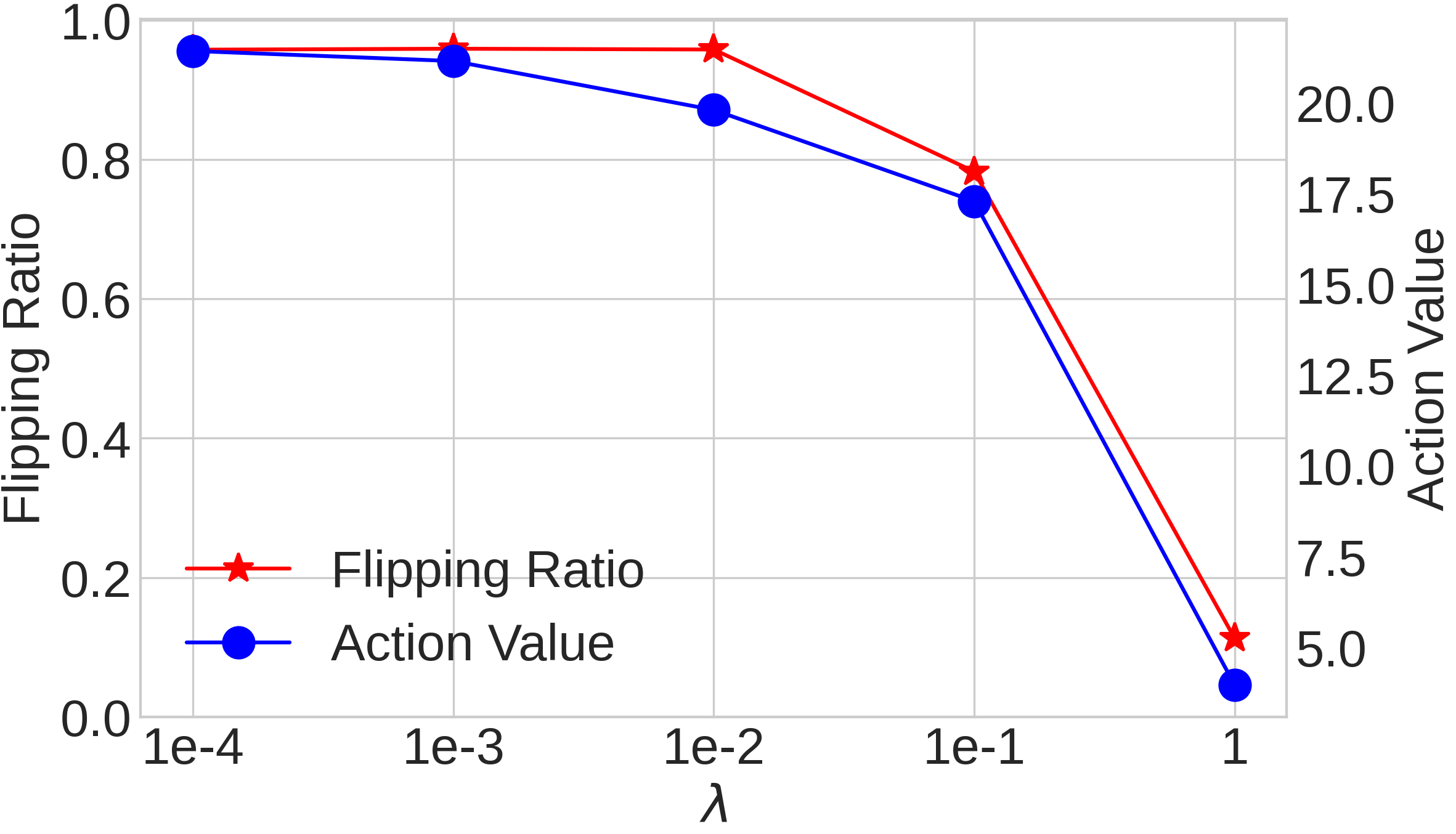
(a) Linear

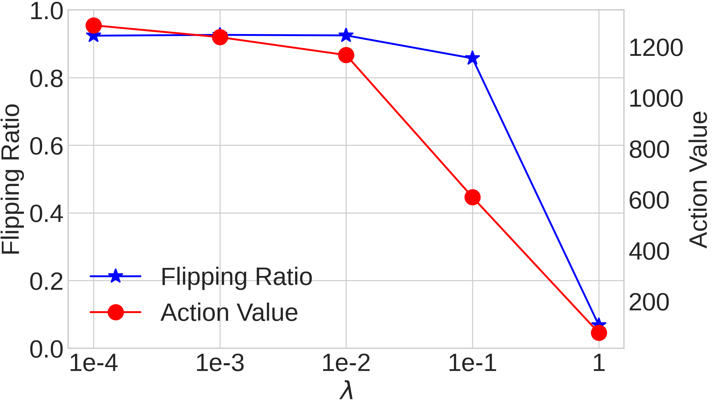
(b) Lotka-Volterra

Figure 3. Effects of the hyperparameter $\lambda$ in Eq. (12).

The objective function (Equation (12)) for training RecAD employs the hyperparameter $\lambda$ to balance the flipping ratio and action value. As shown in Figure 3, on both synthetic datasets, we have similar observations that with the increasing of $\lambda$, both action value and flipping ratio decrease. A large $\lambda$ indicates a large penalty for high action values, which could potentially hurt the performance of flipping abnormal time steps as small action values may not be sufficient to flip the anomalies.

5.2.5. Case Study

We further conduct case studies to show how to use the recourse action predicted by RecAD as an explanation for anomaly detection in multivariate time series.

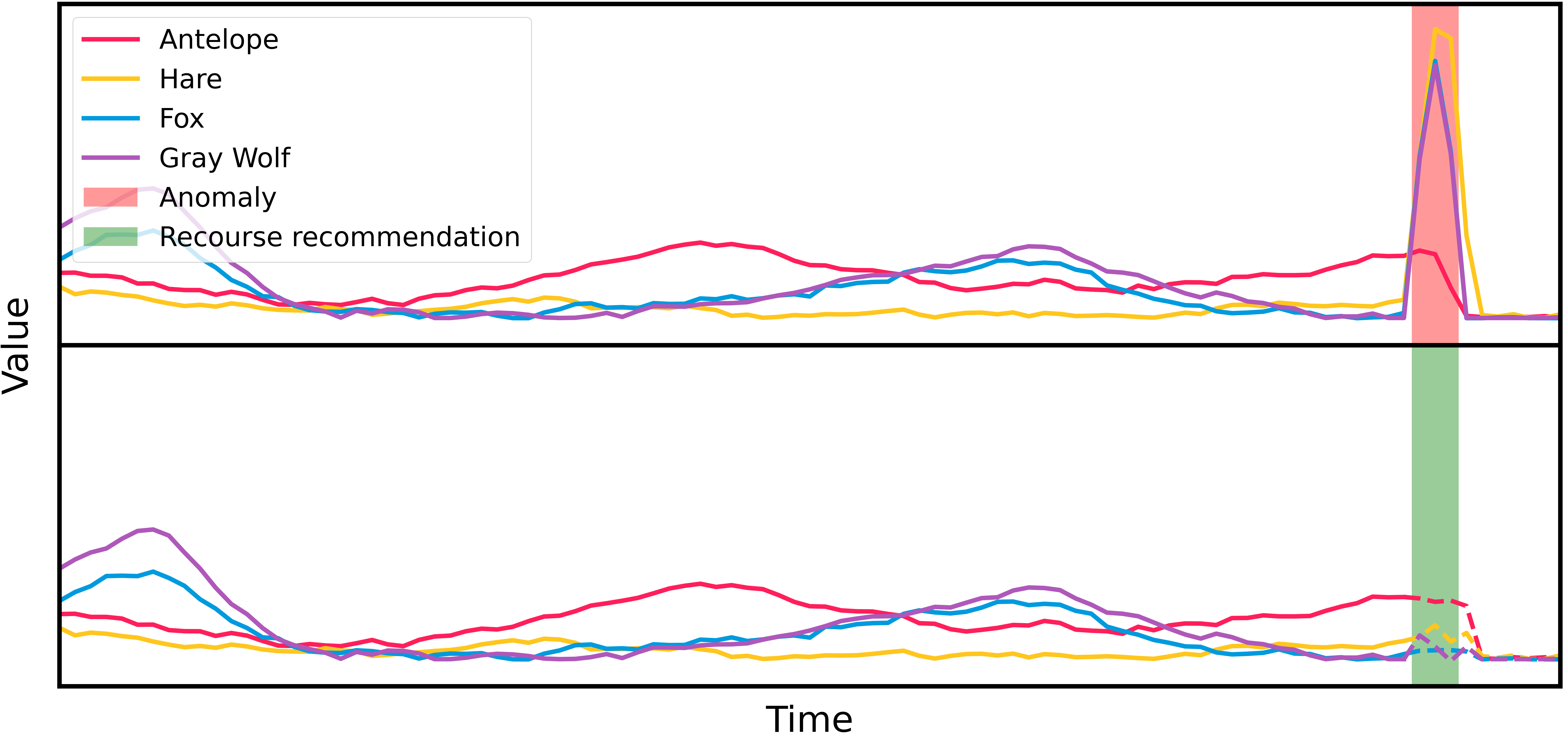
Figure 4. Recourse recommendations for intervening in an imbalanced ecosystem to restore balance.

Case study on the Lotka-Volterra dataset. Figure 4 shows a simulation of a prairie ecosystem that contains antelope, hare, fox, and gray wolf based on the Lotka-Volterra model (Bacaër, 2011), where each time series indicates the population of a species. As shown in the top figure, in most of the time steps, the numbers of carnivores (fox and gray wolf) and herbivores (antelope and hare) keep stable in a balanced ecosystem, say 0.1k-1k antelopes, 1k-10k hares, 0.1k-1k foxes, and 0.1k-1k gray wolves. After detecting abnormal behavior at a specific time step (red area in the top figure), the algorithmic recourse aims to provide recourse actions to flip the abnormal outcome. In this case, the algorithmic recourse model recommends the intervention of reducing the populations of hares, foxes, and gray wolves by 100.1k, 9.3k, and 7.5k, respectively. After applying the recourse actions (green area in the bottom figure), we can notice the populations of four species become stable again (the dashed line in the bottom figure). Therefore, the recourse actions can provide recommendations to restore the balance of the prairie ecosystem.

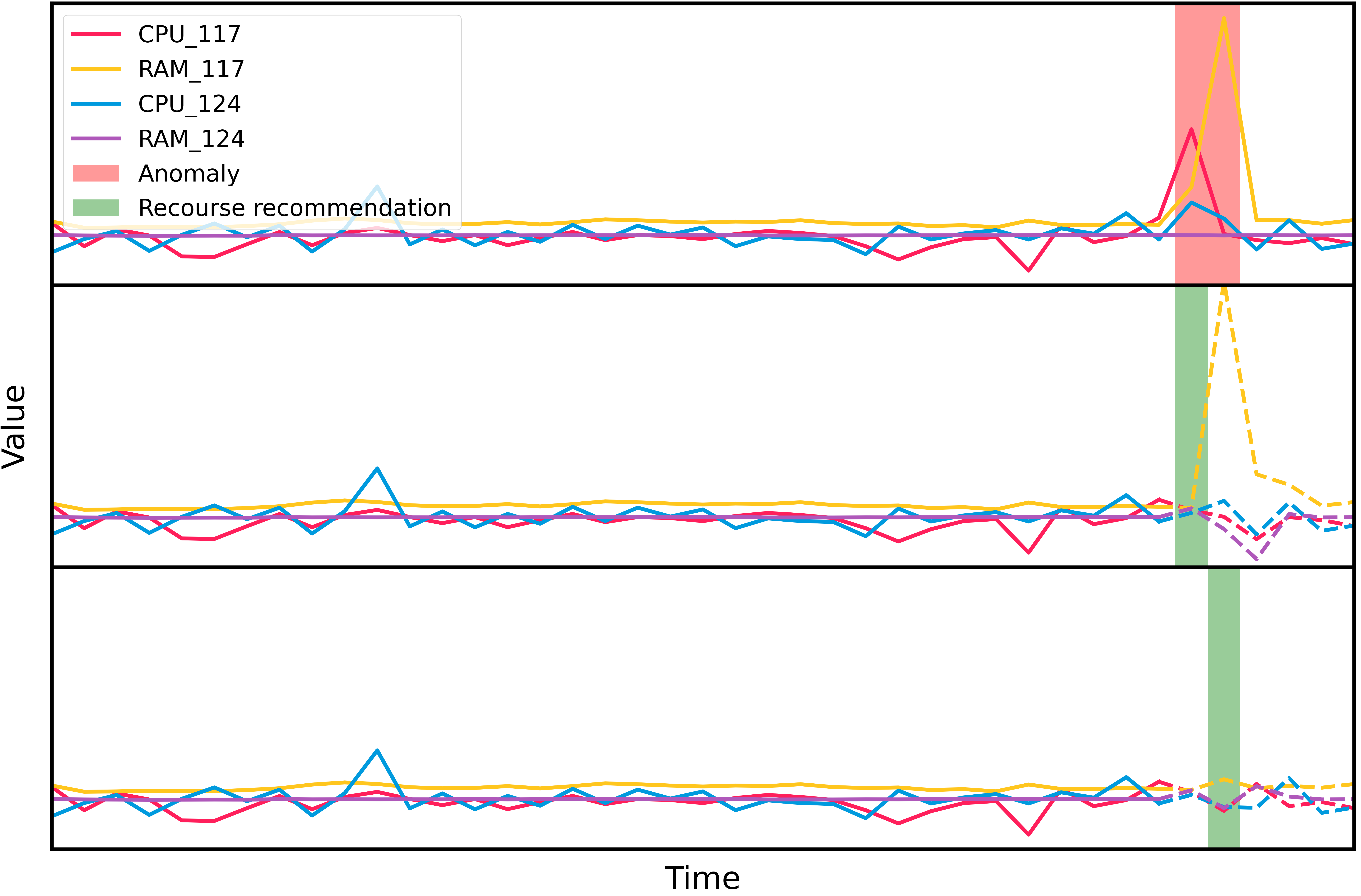
Figure 5. Recourse recommendations for restoring the abnormal CPU and RAM usages in MSDS.

Case study on the MSDS dataset. Figure 5 depicts a case study on MSDS with control nodes 117 and 124. USAD detects a subsequence of anomaly consisting of two abnormal time steps from two time series (CPU and RAM usages on node 117), highlighted in the red area of the top figure.

When the first abnormal time step is detected, RecAD suggests releasing the CPU usage by 6.7 on node 117 (the green area in the middle figure). In other words, it also means the anomaly here is due to the higher CPU usage than normal with a value of 6.7. After taking this action, the following time steps are affected by this action. A counterfactual time series is then generated using the AAP process, which is shown as the dashed lines in the middle of Figure 5. RecAD continues to monitor subsequent time steps for any abnormalities.

The following time step is still detected as abnormal in the time series of memory usage of node 117. RecAD recommends releasing the RAM usage by 13.39 on node 117 (the green area in the bottom figure), meaning that the abnormal time step here is due to high memory usage in a margin of 13.39. After taking the recourse action, the counterfactual time series is then generated (the dashed lines in the bottom figure). We can then observe that the entire time series returns to normal.

In summary, recourse actions recommended by RecAD can effectively flip the outcome and lead to a normal counterfactual time series. Meanwhile, based on the recourse actions, the domain expert can understand why a time step is abnormal.

6. Conclusions

In this work, we have developed a novel framework for algorithmic recourse in time series anomaly detection, called RecAD, which can recommend recourse actions to fix anomalies with the minimum cost. To recommend proper actions with the consideration of the downstream impact of the intervention on the current time step, we leverage Granger causality to model the interdependence in multivariate time series and derive the counterfactual time series based on the Abduction-Action-Prediction process. The empirical studies have demonstrated the effectiveness of RecAD for recommending recourse actions in time series anomaly detection.

References

- (1)
- Audibert et al. (2020) Julien Audibert, Pietro Michiardi, Frédéric Guyard, Sébastien Marti, and Maria A Zuluaga. 2020. Usad: Unsupervised anomaly detection on multivariate time series. In KDD.
- Bacaër (2011) Nicolas Bacaër. 2011. A short history of mathematical population dynamics. Vol. 618. Springer.
- Blázquez-García et al. (2021) Ane Blázquez-García, Angel Conde, Usue Mori, and Jose A Lozano. 2021. A review on outlier/anomaly detection in time series data. In ACM CSUR. 1–33.
- Cook et al. (2019) Andrew A Cook, Göksel Mısırlı, and Zhong Fan. 2019. Anomaly detection for IoT time-series data: A survey. IEEE Internet of Things Journal 7, 7 (2019), 6481–6494.
- Dahlhaus and Eichler (2003) Rainer Dahlhaus and Michael Eichler. 2003. Causality and Graphical Models in Time Series Analysis. Oxford Statistical Science Series (2003), 115–137.
- Datta et al. (2022) Debanjan Datta, Feng Chen, and Naren Ramakrishnan. 2022. Framing Algorithmic Recourse for Anomaly Detection. In KDD. 283–293.
- Dominguez-Olmedo et al. (2022) Ricardo Dominguez-Olmedo, Amir H Karimi, and Bernhard Schölkopf. 2022. On the adversarial robustness of causal algorithmic recourse. In ICML. 5324–5342.
- Granger (1969) Clive WJ Granger. 1969. Investigating Causal Relations by Econometric Models and Cross-Spectral Methods. Econometrica: journal of the Econometric Society (1969), 424–438.
- Karimi et al. (2022) Amir-Hossein Karimi, Gilles Barthe, Bernhard Schölkopf, and Isabel Valera. 2022. A survey of algorithmic recourse: contrastive explanations and consequential recommendations. In ACM CSUR. 1–29.
- Karimi et al. (2021) Amir-Hossein Karimi, Bernhard Schölkopf, and Isabel Valera. 2021. Algorithmic recourse: from counterfactual explanations to interventions. In ACM FAccT. 353–362.
- Karimi et al. (2020) Amir-Hossein Karimi, Julius Von Kügelgen, Bernhard Schölkopf, and Isabel Valera. 2020. Algorithmic recourse under imperfect causal knowledge: a probabilistic approach. In NeurIPS. 265–277.
- Lütkepohl (2005) Helmut Lütkepohl. 2005. New introduction to multiple time series analysis. Springer Science & Business Media.
- Marcinkevičs and Vogt (2021) Ričards Marcinkevičs and Julia E Vogt. 2021. Interpretable models for granger causality using self-explaining neural networks. arXiv preprint arXiv:2101.07600 (2021).
- Nauta et al. (2019) Meike Nauta, Doina Bucur, and Christin Seifert. 2019. Causal Discovery with Attention-Based Convolutional Neural Networks. In MAKE. 312–340.
- Nedelkoski et al. (2020) Sasho Nedelkoski, Jasmin Bogatinovski, Ajay Kumar Mandapati, Soeren Becker, Jorge Cardoso, and Odej Kao. 2020. Multi-source distributed system data for ai-powered analytics. In ESOCC. 161–176.
- Pearl (2009) Judea Pearl. 2009. Causality. Cambridge university press.
- Ren et al. (2019) Hansheng Ren, Bixiong Xu, Yujing Wang, Chao Yi, Congrui Huang, Xiaoyu Kou, Tony Xing, Mao Yang, Jie Tong, and Qi Zhang. 2019. Time-series anomaly detection service at microsoft. In KDD. 3009–3017.
- Ruff et al. (2021) Lukas Ruff, Jacob R Kauffmann, Robert A Vandermeulen, Grégoire Montavon, Wojciech Samek, Marius Kloft, Thomas G Dietterich, and Klaus-Robert Müller. 2021. A unifying review of deep and shallow anomaly detection. Proc. IEEE 5 (2021), 756–795.
- Schmidl et al. (2022) Sebastian Schmidl, Phillip Wenig, and Thorsten Papenbrock. 2022. Anomaly detection in time series: a comprehensive evaluation. In VLDB.
- Shipmon et al. (2017) Dominique T Shipmon, Jason M Gurevitch, Paolo M Piselli, and Stephen T Edwards. 2017. Time series anomaly detection; detection of anomalous drops with limited features and sparse examples in noisy highly periodic data. arXiv preprint arXiv:1708.03665 (2017).
- Tank et al. (2021) Alex Tank, Ian Covert, Nicholas Foti, Ali Shojaie, and Emily B Fox. 2021. Neural granger causality. In IEEE PAMI. 4267–4279.
- Tuli et al. (2022) Shreshth Tuli, Giuliano Casale, and Nicholas R. Jennings. 2022. TranAD: Deep Transformer Networks for Anomaly Detection in Multivariate Time Series Data. In VLDB.
- von Kügelgen et al. (2022) Julius von Kügelgen, Amir-Hossein Karimi, Umang Bhatt, Isabel Valera, Adrian Weller, and Bernhard Schölkopf. 2022. On the fairness of causal algorithmic recourse. In AAAI.