Magnetically Induced Schrödinger Cat States: The Shadow of a Quantum Space

Abstract

Schrödinger cat states, which are superpositions of macroscopically distinct states, are potentially critical resources for upcoming quantum information technologies. In this paper, we introduce a scheme to generate entangled Schrödinger cat states in a non-relativistic electric dipole system situated on a two-dimensional plane, along with an external potential and a uniform strong magnetic field perpendicular to the plane. Additionally, our findings demonstrate that this setup can lead to the phenomenon of collapse and revival of entanglement for a specific range of our model parameters.

I Introduction

In quantum theory, the transition between the microscopic and macroscopic worlds is one of the less-understood features Zuk . Such a transition plays a direct role in the realm of quantum measurements. In an ideal measurement paradigm, the interaction of macroscopic equipment and a microscopic system yields entanglement and a superposed quantum state with both macroscopic and microscopic components pn2 . Schrödinger was the first to highlight the physical subtleties of this kind of superposition by replacing the macroscopic part of the system by a “cat”, in order to illustrate a dramatic superposition of “states” of both alive and dead cats, that should, in practice, be distinguished macroscopically par . The superposition of macroscopically different quantum states, generically referred to as non-classical Schrödinger Cat State (SCS) par ; 2 ; bose , is crucial for understanding the conceptual underpinnings of quantum physics, especially with reference to wave function collapse models pnr ; pr ; hr ; hr1 . In recent years, the advancement of quantum technologies has brought into sharp focus the utility of several quantum phenomena such as photon anti-bunching Rov , sub-Poissonian statistics mar and squeezing mtw , along with the dynamics of SCS.

The success of quantum information theory and its potential applications qinform ; qinf that significantly outperform their classical equivalents have recently sparked a renewed interest in the generation of non-classical states such as SCS. Several applications of cat states have been suggested in the realm of quantum information qinfor , quantum metrology qmeter , quantum teleportation qteleport , and quantum error correction schemes qerror1 ; qerror2 . Besides, the concept of decoherence between two superposed quantum objects, or the quantum-to-classical transition, can be studied using the SCS as a platform. In quantum optics, a superposition of two diametrically opposite coherent states $|\pm\alpha>$ with large value of $\mid\alpha\mid$, can be interpreted as a quantum superposition of two macroscopically distinct states, i.e., a Schrödinger cat-like state tw ; legg . However, due to decay of their interference properties, it is extremely difficult to detect such states in practice egg . Nonetheless, the universality of SCS enables it to be realized in a wide variety of physical arenas such as nonlinear quantum optics Sb , quantum dot systems kaku , superconducting cavities kau , Bose Einstein condensates (BEC) goenner and quantization of weak gravity rbm ; wolf ; sch . A fascinating direction of research in recent years has been the mechanism for the natural generation of SCS in some specific condensed matter systems sch1 ; sch2 .

Schrödinger cat states with entanglement based protocols provide a novel technique to explore short-distance quantum physics in a non-relativistic domain when there is a magnetic dipole interaction background ed . At extremely short distances, the space-time structure needs to be “granular” in order to account for both gravity and quantum uncertainty ein . A viable approach towards quantum gravity is through quantizing space-time itself in , rather than the construction of an effective field theory of gravity. This approach is an active area of research on quantum gravity, commonly referred to as non-commutative geometry go ; pe . The fundamental goal is to derive classical geometry from a suitable limit of a non-commutative algebra. Though such a proposal may appear as ad-hoc pek , the physical justification for such a non-commutative space-time is strong since it provides a solution to the geometric measurement problem near the Planck scale.

Non-commutative geometry appears naturally in various non-relativistic planar systems. For instance, it occurs using the lowest Landau-level (LLL) projection to study the behavior of charged particles in a strong magnetic field ek . Further, the incompressibility of fractional quantum Hall fluids qhefluids has a strong connection to the emergence of a non-commutative geometry in which the fundamental Planck length is substituted by the magnetic length. Non-commutative space-time forms an alternative paradigm for studying the behavior of relativistic anyonic systems in interaction with the ambient electromagnetic field vpn ; Rabin . Additionally, non-commutative properties of real-space coordinates in the presence of the Berry curvature k produce skew scattering by a non-magnetic impurity without relativistic spin-orbit interactions in a condensed matter system. Non-commutative space provides a paradigm for describing the behavior of the quantum to classical transition under the influence of decoherence fg1 ; fg2 , which is relevant for implementation of quantum information protocols. From an experimental standpoint, there have been efforts in search of evidence of possible non-commutative effect manifestations in cosmology and high-energy physics kk ; c ; d . A testable framework has been suggested in low-energy experiments in the arena of quantum Hall effect qhe ; e .

The motivation for the present study is to investigate whether multi-component entangled non-classical SCS could be produced in deformed quantum space, where non-commutativity arises naturally in an easily accessibly low energy physical system. In this article, we investigate the phenomenology of a two-particle electric dipole model with an additional harmonic interaction and a strong background magnetic field, with motion constrained to the plane perpendicular to the field. Such a system may be considered as a toy version of a real Excitonic dipole set-up exci . By exploring the high magnetic field limit, we reveal the emergence of planar non-commutative space as a natural consequence. Furthermore, we establish the deformed Heisenberg algebra as the origin of multi-component entangled SCS in this system. Moreover, we quantify the degree of entanglement of our SCS, and show that the phemomenon of collapse and revival of entanglement R1 ; yueberly ; R2 occurs in this system under the influence of the harmonic potential.

The organization of our paper is as follows. The interacting two particle electric dipole system is introduced in Section 2, showing how classical non-commutative space appears in the presence of a very strong, constant, uniform magnetic field. Then, in Section 3, we move on to the quantum picture, where intricacies of the system dynamics are revealed, in context of mapping between two reference frames. Section 4 discusses how our model with a harmonic oscillator potential that is dependent only on one spatial variable is able to generate entangled multi-component Schrödinger cat states. In Section 5, we compute the degree of entanglement in the generated SCS system and demonstrate that it exhibits the phenomenon of entanglement collapse and revival. Section 6 is reserved for concluding remarks and discussions.

II Two-Particle System: Classical picture

We begin by considering a pair of non-relativistic, oppositely charged particles with equal mass $m$ moving on the plane subjected to a constant magnetic field $B$ along the $z$ axis (ignoring Coulomb and radiation effects). In component form, $x_{i}$ and $y_{i}$ $(i=1,2)$ correspondingly represents the positive and negative charge coordinates. The $z$ coordinate can be suppressed since the dynamics of the system is confined in a plane. Standard Lagrangian in C.G.S. units is used to define the system as follows Dunne ; bag ; pn :

$$L=\frac{1}{2}m(\dot{x}_{i}^{2}+\dot{y}_{i}^{2})+\frac{eB}{2c}\epsilon_{ij}(x_{j}\dot{x}_{i}-y_{j}\dot{y}_{i})$$

$$-\frac{K_{0}}{2}(x_{i}-y_{i})^{2}-V({x_{1}});~{}~{}~{}i,j=1,2$$ (1)

where $c$ is the speed of light in vacuum and $K_{0}$ is the spring constant corresponding to the harmonic interaction between the two oppositely charged particles. This model is constructed in the spirit of the “2D excitonic dipole model” exmol ; emg ; dipex , wherein $m$ can be realized by the effective mass of the “electron-hole” pair in some specific cases where the magnitude of the effective mass of electrons and holes can be considered as approximately same and the Fermi velocity provides an upper bound for its characteristic velocity in a real physical solid state system. Note that the first term of the above Lagrangian (1) represents the kinetic term of the charges and the second term represents their interaction with the external magnetic field $\vec{B}$. We use a rotationally symmetric gauge to define the vector potential $\vec{A}$ satisfying the equation $\vec{\nabla}\times\vec{A}=B\hat{z}$. The third term is the harmonic interaction between the two charges, and finally, the fourth term describes the additional interaction of the positive charge with an impurity in the $x_{1}$ direction. The limit of a strong magnetic field $B$ and small mass $m$ such as $\frac{m}{eB}\rightarrow 0$ is of interest here, in which the kinetic energy term becomes negligible in the Lagrangian (1) BD . Thus, we may approximate the dynamics by the effective Lagrangian,

$$L_{0}=\frac{eB}{2c}\epsilon_{ij}(x_{j}\dot{x}_{i}-y_{j}\dot{y}_{i})-V_{0}(x_{i},y_{i})$$ (2)

where $V_{0}(x_{i},y_{i})=\frac{K_{0}}{2}(x_{i}-y_{i})^{2}+V({x_{1}})$.

The Lagrangian equations of motion of the co-ordinates of the positive and negatively charged particles are given by,

$$\dot{x}_{i}=\frac{c}{eB}\epsilon_{ij}\frac{\partial V_{0}}{\partial x_{j}},~{}~{}\dot{y}_{i}=-\frac{c}{eB}\epsilon_{ij}\frac{\partial V_{0}}{\partial y_{j}}$$ (3)

Since our effective Lagrangian (2) is in first-order form, the effective Hamiltonian of the model is given by

$$H=V_{0}(x_{i},y_{i})$$ (4)

In order to show the equivalence between the Lagrangian and Hamiltonian formalism fj ; Rb , we consider Hamilton’s equations of motion:

$$\dot{x}_{i}=\{{x_{i},H}\}={\{x_{i},V_{0}(x_{i},y_{i})}\}$$ (5)

$$\dot{y}_{i}=\{{y_{i},H}\}={\{y_{i},V_{0}(x_{i},y_{i})}\}$$ (6)

The nontrivial symplectic structure can readily be obtained now by comparing the Lagrangian equations of motion (3) with the form of Hamilton’s equations of motion ($\ref{a1},\ref{a2}$) to yield the following brackets:

$$\{x_{i},x_{j}\}=\frac{c}{eB}\epsilon_{ij};~{}~{}\{y_{i},y_{j}\}=-\frac{c}{eB}\epsilon_{ij};~{}~{}\{y_{i},x_{j}\}=0$$ (7)

The canonical spatial translation generators for individual charged particles are given by

$$P_{x_{i}}=\frac{eB}{c}\epsilon_{ij}x_{j};~{}~{}P_{y_{i}}=-\frac{eB}{c}\epsilon_{ij}y_{j}$$ (8)

Using the above expressions and the nontrivial symplectic structures between the position co-ordinates (7), it can be checked that the momentum co-ordinates also satisfy a nontrivial symplectic bracket, given by

$$\{P_{x_{i}},P_{x_{j}}\}=\frac{eB}{c}\epsilon_{ij};~{}~{}\{P_{y_{i}},P_{y_{j}}\}=-\frac{eB}{c}\epsilon_{ij};~{}~{}$$

$$\{x_{i},P_{x_{j}}\}=\{y_{i},P_{y_{j}}\}=\delta_{ij}$$ (9)

III Quantum dynamics

In this section, we discuss the quantum theory of our non-relativistic two-particle model at the strong magnetic field limit by elevating the phase space variables to the level of quantum operators. We obtain the nontrivial or unusual commutation brackets between the position operators given by:

$$[\hat{x}_{i},\hat{x}_{j}]=il^{2}_{B}\epsilon_{ij};~{}~{}[\hat{y}_{i},\hat{y}_{j}]=-il^{2}_{B}\epsilon_{ij};~{}~{}[\hat{x}_{i},\hat{y}_{j}]=0;~{}~{}i,j=1,2$$ (10)

with $l_{B}=\sqrt{\frac{\hbar c}{eB}}$ known as the magnetic quantum length scale. Likewise, the other nontrivial phase space non-commutative algebras are given as

$$[\hat{P}_{x_{i}},\hat{P}_{x_{j}}]=i\frac{\hbar^{2}}{l^{2}_{B}}\epsilon_{ij};~{}~{}[\hat{P}_{y_{i}},\hat{P}_{y_{j}}]=-i\frac{\hbar^{2}}{l^{2}_{B}}\epsilon_{ij},$$ (11)

$$[\hat{x}_{i},\hat{P}_{x_{j}}]=[\hat{y}_{i},\hat{P}_{y_{j}}]=i\hbar\delta_{ij};$$ (12)

It may be observed that in this case, neither the coordinates nor the momentum operators commute pnb2 . However, the operators

$$\hat{P}_{i}=\hat{P}_{x_{i}}+\hat{P}_{y_{i}}=\frac{eB}{c}\epsilon_{ij}(\hat{x}_{j}-\hat{y}_{j}),$$ (13)

can act as proper (commutative) translation generators, so that they satisfy the following commutation relations:

$$[\hat{x}_{i},\hat{x}_{j}]=il^{2}_{B}\epsilon_{ij};~{}~{}[\hat{P}_{i},\hat{P}_{j}]=0;~{}~{}[\hat{x}_{i},\hat{P}_{j}]=i\hbar\delta_{ij},$$ (14)

which represents a non-commutative Heisenberg algebra (NCHA) in two dimensions. In this instance, the operator-valued Hamiltonian of the effective system is given by

$$\hat{H}=\frac{K_{0}}{2}(\hat{x}_{i}-\hat{y}_{i})^{2}+V(\hat{x}_{1})$$ (15)

A more conventional setting of this Hamiltonian in terms of the commutative translation generator $\hat{P}_{i}$ is as follows:

$$\hat{H}=\frac{1}{2m_{B}}\hat{P}^{2}_{i}+V(\hat{x}_{1});~{}~{}~{}i=1,2$$ (16)

where $m_{B}=\frac{e^{2}B^{2}}{c^{2}K_{0}}$ is the effective mass of the reduced two-particle system. It turns out to be instructive to introduce the pair of canonical variables:

$$\hat{R}_{i}=\frac{\hat{x}_{i}+\hat{y}_{i}}{2};~{}~{}\hat{P}_{i}=\frac{eB}{c}\epsilon_{ij}(\hat{x}_{j}-\hat{y}_{j});~{}~{}i,j=1,2$$ (17)

where $\hat{R}_{i}$ is the centre of mass coordinate and $\hat{P}_{i}$ is the corresponding canonical momentum of our two-particle system. They satisfy the usual Heisenberg commutation relations as

$$[\hat{R}_{i},\hat{R}_{j}]=0;~{}~{}[\hat{P}_{i},\hat{P}_{j}]=0;~{}~{}~{}[\hat{R}_{i},\hat{P}_{j}]=i\hbar\delta_{ij}$$ (18)

However, it is worth noting that the centre of mass position coordinates may also satisfy non-commutative Heisenberg algebra (NCHA) if the two particles are assumed to have different masses (For further details, see Appendix A). Even, if the two particles have the same mass, but their position coordinates satisfy NCHA with different non-commutativity parameters, in that case also, the centre of mass position coordinates can give rise to a non-commutative algebra.

Note further, that since the dynamics of the composite system is realized in terms of the coordinates of the positively charged particle, the information of the negatively charged particle is completely suppressed in the equations (14, 16), but it is incorporated into the expression of commuting momentum operators. The extended Heisenberg algebra of the type as considered in eq.(14) has the important property: it is realizable in terms of commutative usual phase space variables (17) as

$$\hat{x}_{1}=Ad_{\hat{U}}(\hat{R}_{1});~{}~{}\hat{P}_{1}=Ad_{\hat{U}}(\hat{P}_{1})$$ (19)

$$\hat{x}_{2}=Ad_{\hat{U}^{\dagger}}(\hat{R}_{2});~{}~{}\hat{P}_{2}=Ad_{\hat{U}^{\dagger}}(\hat{P}_{2})$$ (20)

where we have made use of the fact of adjoint action: $Ad_{\hat{U}}(\hat{A})=\hat{U}\hat{A}\hat{U}^{\dagger}$ with a quasi unitary operator $\hat{U}$:

$$\hat{U}=\exp[(-\frac{il^{2}_{B}}{2\hbar^{2}})\hat{P}_{1}\hat{P}_{2}],$$ (21)

as it does not act unitarily on the entirely non-commutative phase space.

We can observe from the aforementioned equations (19, 20) that the non-commutative phase space commutation algebra (14) can be simulated in terms of commutative phase space variables (canonical variables) i.e. the centre of mass coordinates as

$$\hat{x}_{i}=\hat{R}_{i}-\frac{c}{2eB}\epsilon_{ij}\hat{P}_{j},~{}~{}~{}~{}i,j=1,2$$ (22)

It may be noted that this transformation is not canonical because it changes the commutation brackets. This transformation has occasionally been called a Darboux map n2 or Bopp’s shift hm2 which is of relevance in the Bohmian interpretation of non-commutative quantum mechanics pbom . Furthermore, this transformation with an explicit dependence on the deformation parameter, allows us to convert the Hamiltonian in NC space into a modified Hamiltonian in commutative equivalent space. It follows that if we are able to solve the spectrum of the system Hamiltonian in commutative equivalent space, we can also obtain the spectrum of the system in primitive non-commutative space, though the states in both situations are not the same. We will discuss how the aforementioned maps aid in the extraction of non-classical cat states in the next section.

IV Preparation of Schrödinger Cat states

Using the formalism presented in the previous section, we are now in a position to investigate the main goal of this work, viz., how we might naturally prepare Schrödinger’s Cat states. To do so, we first consider a particular Hamiltonian with a harmonic oscillator potential in the $\hat{x}_{1}$ direction, given by

$$\hat{H}\rightarrow\hat{H}_{NC}=\frac{\hat{P}^{2}_{1}}{2m_{B}}+\frac{\hat{P}^{2}_{2}}{2m_{B}}+V(\hat{x}_{1}),$$ (23)

where $V(\hat{x}_{1})=\frac{1}{2}K\hat{x}^{2}_{1}$ and $m_{B}=\frac{e^{2}B^{2}}{c^{2}K_{0}}$. The corresponding time dependent Schrödinger equation is:

$$i\hbar\frac{\partial}{\partial t}|\psi(t)>_{NC}=\hat{H}_{NC}|\psi(t)>_{NC}$$ (24)

Note that, because of the non-commutativity of this theory, it is impossible to construct simultaneous eigenstates with noncommutative coordinates, which makes it difficult to define a local probability density for the wave-function that corresponds to a particular state $|\psi(t)>_{NC}$ pbom1 . However, this issue can be bypassed by using the interpretation mentioned in pbom1 , or by using the coherent states formulation of noncommutative quantum mechanics with the help of the Voros product g .

In our present case, it can be easily observed that the system Hamiltonian mentioned above can be rewritten as,

$$\hat{H}_{NC}=\hat{U}\hat{H}_{CM}\hat{U}^{\dagger},$$ (25)

with

$$\hat{H}_{CM}=\frac{\hat{P}^{2}_{1}}{2m_{B}}+\frac{\hat{P}^{2}_{2}}{2m_{B}}+V(\hat{R}_{1}),$$ (26)

where we have used the fact that $V(\hat{x}_{1})=V(\hat{U}\hat{R}_{1}\hat{U}^{\dagger})=\hat{U}V(\hat{R}_{1})\hat{U}^{\dagger}$. Here $\hat{H}_{CM}$ is the unitarily equivalent form of the system Hamiltonian expressed in terms of the Center of Mass coordinates, whereas the $\hat{H}_{NC}$ represents the system Hamiltonian written in terms of the positively charged particle coordinates. We can readily recognize that $V(\hat{R}_{1})=\frac{1}{2}K\hat{R}^{2}_{1}$, where $K$ is the spring constant of the impurity interaction faced by the positive charge in the $\hat{x}_{1}$ direction only. Accordingly, the Schrödinger equation (24) transforms as follows:

$$i\hbar\frac{\partial}{\partial t}|\psi(t)>_{CM}=\hat{H}_{CM}|\psi(t)>_{CM}$$ (27)

where $|\psi(t)>_{CM}=\hat{U}^{\dagger}|\psi(t)>_{NC}.$ The ground state of the unitarily equivalent Hamiltonian ($\hat{H}_{CM}$) is now represented as

$$|\psi_{0}>_{CM}=|0>\otimes[d_{+}|+k_{2}>+d_{-}|-k_{2}>],$$ (28)

where $|d_{+}|^{2}$ and $|d_{-}|^{2}$ denote the probability of finding the free particle in $|+k_{2}>$ and $|-k_{2}>$ states respectively, $|0>$ represents the ground state of the 1D harmonic oscillator system with $\hat{a}_{1}$ and ${\hat{a}_{1}}^{\dagger}$ representing the corresponding annihilation and creation operators respectively, satisfying the following algebra:

$$[\hat{a}_{1},\hat{a}^{\dagger}_{1}]=\mathbb{I};~{}~{}~{}~{}\hat{a}_{1}=\frac{m_{B}\omega_{B}\hat{R}_{1}+i\hat{P}_{1}}{\sqrt{2m_{B}\omega_{B}\hbar}};~{}~{}~{}~{}~{}\hat{a}_{1}|0>=0,$$ (29)

with $\omega_{B}=\sqrt{\frac{K}{m_{B}}}$, and $|\pm k_{2}>$ corresponds to the right and left moving free particle’s momentum state respectively, which satisfies:

$$\hat{P}_{2}|\pm k_{2}>=\pm P_{2}|\pm k_{2}>;~{}~{}~{}~{}P_{2}=\hbar k_{2}$$ (30)

The state vector corresponding to the non-commutative phase space (or in terms of the positively charged particle coordinates) is given by

$$|\psi_{0}>_{NC}=\hat{U}|\psi_{0}>_{CM},$$ (31)

$|\psi_{0}>_{NC}$ can be expressed as,

$$|\psi_{0}>_{NC}=(\exp[(-\frac{il^{2}_{B}}{2\hbar^{2}})\hat{P}_{1}\otimes\hat{P}_{2}])$$

$$[|0>\otimes(d_{+}|+k_{2}>+d_{-}|-k_{2}>)]$$ (32)

which leads to

$$|\psi_{0}>_{NC}=d_{+}([\exp(-\frac{il^{2}_{B}k_{2}}{2\hbar}\hat{P}_{1})]|0>)\otimes|+k_{2}>$$

$$+d_{-}([\exp(\frac{il^{2}_{B}k_{2}}{2\hbar}\hat{P}_{1})]|0>)\otimes|-k_{2}>$$ (33)

On substituting $l^{2}_{B}=\frac{\hbar c}{eB}$ in the above equation, we arrive at-

$$|\psi_{0}>_{NC}=d_{+}([\exp[{(-i\frac{ck_{2}}{2eB})}\hat{P}_{1}]]|0>)\otimes|+k_{2}>$$

$$+d_{-}([\exp[(i\frac{ck_{2}}{2eB})\hat{P}_{1}]]|0>)\otimes|-k_{2}>$$ (34)

Now, for a harmonic oscillator potential, the momentum operator $\hat{P}_{1}$ can be written as-

$$\hat{P}_{1}=i\sqrt{\frac{m_{B}\omega_{B}\hbar}{2}}({\hat{a}_{1}}^{\dagger}-\hat{a}_{1})$$ (35)

Putting the above expression in equation (33), we obtain,

(36)

It follows that the above state vector (36) may also be written in the form of a superposition of single-component coherent states as

$$\scalebox{0.8}{$|\psi_{0}>_{NC}=d_{+}|+\alpha>\otimes|+k_{2}>+d_{-}|-\alpha>\otimes|-k_{2}>$},$$ (37)

wherein $|\pm\alpha>=e^{\pm\alpha({\hat{a}_{1}}^{\dagger}-\hat{a}_{1})}|0>$ with $\alpha=\frac{ck_{2}}{2eB}\sqrt{\frac{m_{B}\omega_{B}\hbar}{2}}$ are real-valued coherent states (or a displacement of the vacuum) that belong to the subset of the over complete space of usual complex parameter valued coherent states bom1 .

Here it may be worthwhile to mention a property of the coherent state $|\pm\alpha>$: the dimensionless parameter $\alpha$ may be rewritten as

$$\alpha=\frac{1}{2}P_{2}({\frac{K}{K_{0}}})^{1/4}\sqrt{\frac{c}{2eB\hbar}}=\xi k_{2}l_{B}$$ (38)

with $\xi=\frac{1}{2}(\frac{K}{4K_{0}})^{\frac{1}{4}}$ . A coherent state $|\alpha>$ can have an arbitrarily large amplitude, and hence, the energy of a macroscopic harmonic oscillator scv can be approximated by the energy of a one-dimensional quantum mechanical HO by suitably choosing $\mid\alpha\mid$ to be arbitrarily large. For large enough $\mid\alpha\mid$ values, $|+\alpha>$ and $|-\alpha>$ correspond to macroscopically distinguishable states and may be labelled as ‘(+) (alive)’ and ‘(-) (dead)’ sv ; gl . In this sense, we can regard the above state (37) as an entangled SCS, holding $\mid\alpha\mid\sqrt{h}$ fixed with finite value in the classical limit v ; s . Accordingly, one may consider $|\pm\alpha>$ to be “classical-like” states, but their coherent superposition is endowed with non-classical properties. In fact, this type of Schrödinger cat states have been generated by pulsed stimulation of atomic Rydberg wave packets vn .

In the primitive non-commutative phase space, we may rewrite the state vectors (36) in the following concise way:

$$|\psi_{0}>_{NC}=\mathcal{N}[|+\alpha;+k_{2}>+e^{i\phi}|-\alpha;-k_{2}>];~{}~{}$$

$$|\pm\alpha;\pm k_{2}>=|\pm\alpha>\otimes|\pm k_{2}>,$$ (39)

with an arbitrary phase factor ($\phi$) and normalization constant $\mathcal{N}$. For the aforementioned reason, the states $|\pm\alpha>$ may be considered to be “macroscopic” like states with the same amplitude but opposite in phase. (in the present case, the $\mid\alpha\mid$ parameter is not arbitrary, but is defined in terms of the spring constants, magnetic field and electric charge). However, their superposition (39) has several non-classical characteristics op . Particularly, for the relative phase factor $e^{i\phi}=\pm 1$, we get even and odd cat states that have been well-studied in the literature 2 ; bose . Moreover, it is evident from (39) that the coherent states and the free particle states are entangled: when the coherent state parameter has a positive sign, the free particle state is right-moving. On the other hand, the free particle state is left-moving when the coherent state parameter has a negative sign. Therefore, $|\psi_{0}>_{NC}$ is an entangled Schrödinger cat state containing the coherent superposition cohsup1 ; cohsup2 of two states that are diametrically opposite to one another.

Since a momentum eigenstate is an idealization kop , we consider a more realistic scenario in which the system’s motion in the commutative phase space is localized within a specific length scale $\sigma$ along the $\hat{R}_{2}$ direction. In this case, we generalize the notion of free particle states to a propagating Gaussian state given by

$$|\psi_{G}>=\sqrt{\frac{\sigma}{\sqrt{\pi}}}\int_{-\infty}^{+\infty}e^{-\frac{\sigma^{2}}{2}(k_{2}-k_{0})^{2}}|k_{2}>dk_{2}$$ (40)

where $\sigma$ is the width and $k_{0}$ is the peak momentum of the wave packet. Now, following the prescription of (28), we can write the composite state of the particle, when the dynamics of the system are realized in terms of the centre of mass coordinates, as

$$|\psi_{0}>_{CM}=|0>\otimes|\psi_{G}>$$ (41)

Accordingly, we can generalize the notion of a two-component cat state (39) to

(42)

which describes a multi-component entangled Schrödinger cat state rop1 where each component is specified through the momentum eigenvalues. Such a state is highly non-classical, which can be verified through the corresponding Wigner function rop1 . Thus, in the presence of a strong magnetic field background, one may successfully prepare a Schrödinger Cat State utilizing a non-relativistic electric dipole model, where non-commutativity plays an important role. It may be reiterated here that we explore the system in terms of the positively charged particle coordinates.

V Collapse and revival of entanglement of SCS

In this section, we will begin by investigating the degree of entanglement of the SCS state $|\psi>_{NC}$. In order to do so, we first write down the corresponding density matrix given by

$$\hat{\rho}_{NC}=(\sqrt{\frac{\sigma}{\sqrt{\pi}}})^{2}\int_{-\infty}^{+\infty}\int_{-\infty}^{+\infty}[|\alpha(k_{2})>_{A}<\alpha(k_{2}^{\prime})|]$$

$$\otimes[|k_{2}>_{B}<k_{2}^{\prime}|]e^{\frac{-\sigma^{2}}{2}(k_{2}-k_{0})^{2}}e^{\frac{-\sigma^{2}}{2}(k_{2}^{\prime}-k_{0})^{2}}dk_{2}dk_{2}^{\prime}$$ (43)

where the subscripts $A$ and $B$ denote two distinct subsections of our bipartite system, one of which is associated with coherent states and the other with momentum eigenstates, each of which corresponds to two distinct degrees of freedom in the non-commutative plane. Since $|\psi>_{NC}$ is a composite pure state, the entanglement between the coherent states and free particle states can be quantified in terms of the von-Neumann entropy given by

$$S=-Tr_{A}[\hat{\rho}_{red}~{}ln(\hat{\rho}_{red})]$$ (44)

where the reduced density matrix is defined as

$$\hat{\rho}_{red}=\text{Tr}_{B}[\hat{\rho}_{NC}]$$

$$=\frac{\sigma}{\sqrt{\pi}}\int_{-\infty}^{+\infty}[|\alpha(k_{2})>_{A}<\alpha(k_{2})|]e^{-\sigma^{2}(k_{2}-k_{0})^{2}}dk_{2}$$ (45)

with

$$\text{Tr}(\hat{\rho}_{red})=\frac{\sigma}{\sqrt{\pi}}\int_{-\infty}^{+\infty}e^{-\sigma^{2}(k_{2}-k_{0})^{2}}dk_{2}=1$$ (46)

For the present purpose, it suffices to compute the purity function purity , given by

$$\text{P}(\alpha)=\text{Tr}(\hat{\rho}^{2}_{red})=\sum_{n}<n|\hat{\rho}^{2}_{red}|n>$$

$$=\sum_{m}\sum_{n}<n|\hat{\rho}_{red}|m><m|\hat{\rho}_{red}|n>$$ (47)

After a little algebra, one obtains

$$<n|\hat{\rho}_{red}|m>=\frac{\sigma}{\sqrt{\xi^{2}l_{B}^{2}+\sigma^{2}}}\frac{1}{\sqrt{n!}\sqrt{m!}}e^{(-\sigma^{2}k_{0}^{2})}$$

$$(\frac{\xi l_{B}}{2\sigma^{2}})^{n+m}\frac{\partial^{n+m}}{\partial k^{n+m}_{0}}(e^{\frac{\sigma^{4}k_{0}^{2}}{\xi^{2}l_{B}^{2}+\sigma^{2}}})$$ (48)

By inserting equation (V) into (V) it follows that

$$\scalebox{0.9}{$\text{P}(\xi_{0};l_{B})=(\frac{1}{1+\xi^{2}_{0}})e^{(-2\sigma^{2}k_{0}^{2})}[e^{(\frac{\sigma^{2}k_{0}^{2}}{1+\xi_{0}^{2}})}(e^{\frac{\xi^{2}_{0}}{2\sigma^{2}}\overset{\leftarrow}{\frac{\partial}{\partial k_{0}}}\overset{\rightarrow}{\frac{\partial}{\partial k_{0}}}})e^{(\frac{\sigma^{2}k_{0}^{2}}{1+\xi_{0}^{2}})}]$};$$ (49)

where $\xi_{0}=\frac{\xi l_{B}}{\sigma}$. The above expression can be rewritten (see Appendix B) as

$$\text{P}(\xi_{0};l_{B})=\frac{1}{\sqrt{{1+2\xi^{2}_{0}}}}$$ (50)

In Figure 1, we plot the Purity function versus the parameter $\xi_{0}$. It can be observed that the purity function reduces from unit value (separable or disentangled state) with increase of the parameter $\xi_{0}$, indicating increment of entanglement in the system for higher values of $\xi_{0}$ (or lower values of the width of the wave packet $\sigma$). We consider the quantum length scale $l_{B}=1.483\times 10^{-8}$m, and vary the width of the wave-packet in the range of $O(10^{-11}\to 10^{-6})$. Different $l_{B}$ values displayed in the figure may originate due to the variation of the magnetic length scale with different accessible magnetic fields in the laboratory.

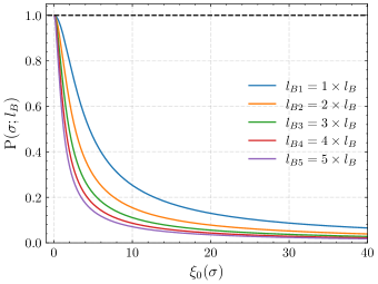
Figure 1: The Purity function is plotted against the dimensionless factor $\xi_{0}$ which varies inversely with the width of the wave-packet $\sigma$. Plots for several choices of the quantum length scale are displayed.

It may be noted that if we just assume $\xi_{0}<<1$ with $\xi\sim 1$ which implies that $l_{B}<<\sigma$, i.e, the width of the Gaussian packet ($\sigma$) is large enough compared to the magnetic quantum length scale such that we can ignore $\xi_{0}$, then it leads to the unit value of the purity function, or in other words, the collapse of the entanglement in the state. On the other hand, we can make the states entangled by choosing $\sigma$ comparable to the magnetic length scale $l_{B}$ where $\text{P}(\xi_{0};B)$ becomes less than unity. More interestingly, the revival of the entanglement state can occur, if one considers a time-dependent regime. Let us recall from the definition of $\xi$, that it basically depends on the coupling strength $K$ of the “impurity” interaction.

The dynamic behaviour of impurities in materials is known to lead to time-varying spring interaction Dj1 ; Dj6 . Such dynamical nature of the coupling has been studied in the literature in the context of several physical systems such as in optical lattices Dj5 , and extensively in the domain of quantum electronic transport Dj ; Dj3 ; Dj4 . Let us now, consider that the spring “constant” $K$ is a slowly varying periodic function of time due to some external effects, with the time-variation given by

$$K(t)=K\text{cos}^{4}\omega_{d}t=K\text{cos}^{4}\theta(t)$$ (51)

which clearly indicates $\xi(t)=\frac{1}{2}(\frac{K\text{cos}^{4}\omega_{d}t}{4K_{0}})^{(1/4)}$ and $\xi_{0}(t)=\frac{\xi(t)l_{B}}{\sigma}$. Hence, the purity function gets modified to,

$$\text{P}(\xi_{0};l_{B})=\frac{1}{\sqrt{1+2{\xi^{2}_{0}(t)}}}$$ (52)

From the above equation, it follows that the Purity function is periodic. It may be noted that even if the $\sigma$ is comparable to the magnetic length scale $l_{B}$, disentanglement occurs for $t_{d}=\frac{\pi}{2\omega_{d}},\frac{3\pi}{2\omega_{d}},\frac{5\pi}{2\omega_{d}},\frac{7\pi}{2\omega_{d}},.....$ with a separation of $\frac{\pi}{\omega_{d}}$ time period between two successive collapses. For the rest of the time interval, the states are entangled. This distinguishing feature is known as the collapse and revival of entanglement in the literature rop2 . In Figure 2, we plot the Purity function versus the periodic parameter $\theta(t)$ for several different values of the wavepacket width $\sigma$. It is clearly seen that the magnitude of entanglement revival increases more for narrower wavepackets.

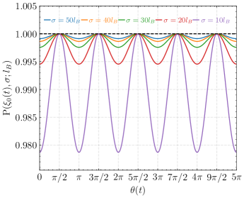
Figure 2: Time evolution of the Purity function is plotted against the parameter $\theta(t)$, for various widths of the wavepackets $\sigma$.

Here it needs to be mentioned that in order to observe entanglement revival of the states, it is required to choose $\sigma$ of the order comparable to that of the magnetic length scale $l_{B}$ or less, as $-1\leq\text{cos}\omega_{d}t\leq+1$. On the other hand, if we choose $\sigma$ to be much larger than $l_{B}$, then the additional term in the denominator of Eq.(52) can be completely negligible which will take us back again to the situation of the entanglement collapse, viz. $\text{P}(\xi_{0};B)\sim 1$. Instances of the phenomenon of entanglement collapse and revival have been pointed out earlier in the literature predominantly in the context of the Jaynes-Cummings model for optical systems R2 ; rop2 . Here we furnish a striking example of entanglement collapse and revival in the context of an excitonic dipole in a condensed matter system.

VI Conclusions

To summarize, in this work, we have considered a composite two-particle planar dipole system in the presence of a strong constant and uniform magnetic field, in which two oppositely charged particles interact via harmonic interaction, in addition to an impurity interaction experienced by the positively charged particle. Our system may be regarded as a toy version of excitonic dipole models that can be realized in some specific direct band gap semiconductors exciband2 ; exciband3 ; exciband1 having the conduction band minimum for electrons and the valence band maximum for holes both located at the same point of the Brillouin zone, where the effective mass of electrons and holes can be quite similar in magnitude. This typically arises due to specific band structures and symmetries of materials. The additional interaction could arise from intrinsic features such as defects or impurities, as well as from external influences like an external electric field or strain in the material e4 .

In our analysis, we have first addressed the classical picture in the context of our system’s Lagrangian formulation which is the most natural in a strong magnetic field limit. Using symplectic analysis of this first-order Lagrangian, we have specified the canonical/Weyl-Moyal type deformed NC classical phase space to be an intrinsic part of our model. Next, we have explored the quantum mechanical description of our model by elevating all the phase space variables to the level of Hermitian operators. The spatial and momentum sectors of individual charged particles obey a non-commutative deformed algebra. Here, the non-commutativity emerges as a natural consequence of placing two oppositely charged particles in a strong constant background magnetic field. The square of the magnetic length scale acts as the effective non-commutative parameter.

We have presented a physical interpretation of the mapping from the deformed phase space to the usual commutative phase space. The non-commutative phase space represents the system Hamiltonian written in terms of the positively charged particle coordinates, while the standard quantum mechanical phase space is more suitable for describing our system in terms of the composite system’s centre of mass coordinates. The dynamics can, therefore, be analyzed in terms of non-commuting variables or, alternatively, using phase space transformations, in terms of commuting variables. In literature, non-commutativity has been often introduced by hand for a single point particle, thus ruling out any physicality of commutative phase-space variables in such cases. However, in the present case, non-commutativity emerges naturally, thereby giving a physical meaning to the commutative phase-space variables. Determining the Hamiltonian’s ground state in the commutative phase space allows us to express the quantum state in the non-commutative phase space as a superposition of two diametrically opposite coherent states, entangled with momentum eigenstates. This reveals the emergence of entangled and two-component as well as multi-component Schrödinger Cat States (SCS) in our system.

Furthermore, we have estimated the magnitude of entanglement in the system of multicomponent entangled cat states. By utilizing the purity function, we demonstrate that the effective non-commutative parameter ($l_{B}^{2}$) is responsible for the entanglement. We show that when the width of the Gaussian wave packet ($\sigma$) significantly exceeds the minimal length scale ($l_{B}$), the entangled cat states undergo collapse. Conversely, when $\sigma$ is comparable to the nonzero magnetic length scale $l_{B}$, the entanglement can be observed. Moreover, we show that if time-dependent impurity potential is chosen, entanglement revival and collapse occurs periodically. So notably, within the same formalism, we observe the phenomenon of collapse and revival of entanglement in the non-commutative plane in the time-dependent regime with a suitable choice of the $\sigma$ parameter for the revival case, while the collapse is completely controlled by the nodes of the periodic function involved in the impurity interaction.

Before concluding, it may be noted that spin-orbit interactions in solid-state systems introduce electronic band curvature, leading to the emergence of Berry curvature in momentum space. Such Berry curvature modifies the usual phase space symplectic structure of Bloch electrons xio ; xio2 . In light of non-commutative quantum mechanics, our present analysis can be extended to include investigations on the possible emergence of Schrödinger cat states in solid state systems involving the 2D excitonic Coulomb problem with the Berry curvature of the electron’s and the hole’s Bloch states Be1 ; Be2 ; Be3 . This may open up a new window to experimentally observe quantum superposition for “macroscopic” states.

VII Acknowledgements

PN and ND acknowledge support from S.N. Bose National Centre for Basic Sciences where this work was initiated. PN would also like to thank the Institute of Theoretical Physics, Stellenbosch University for providing postdoctoral funds during the period when a major part of this work was completed. We thank Biswajit Chakraborty, Debasish Chatterjee, Ananda Dasgupta and Frederik G. Scholtz for some fruitful discussions. ASM acknowledges support from the Project No. DST/ICPS/QuEST/2018/98 from the Department of Science and Technology, Government of India.

VIII Appendix A

Here we present a manifestation of the non-commutativity of the centre of mass coordinates arising in the case of two oppositely charged particles with different masses $m_{+}$ and $m_{-}$ representing the masses of positive and negatively charged particles respectively. The corresponding centre of mass (CM) coordinates of the above-discussed system is-

$$\hat{R}_{i}=\frac{m_{+}\hat{x}_{i}+m_{-}\hat{y}_{i}}{m_{+}+m_{-}};$$

$$~{}\hat{P}_{i}=\hat{P}_{x_{i}}+\hat{P}_{y_{i}}=\frac{eB}{c}\epsilon_{ij}(\hat{x}_{j}-\hat{y}_{j});~{}~{}i,j=1,2$$ (53)

Now, utilizing the results obtained from equation (10), the commutation brackets between the CM coordinates can be obtained in the following form-

$$[\hat{R}_{i},\hat{R}_{j}]=\frac{m_{+}^{2}-m_{-}^{2}}{(m_{+}+m_{-})^{2}}il_{B}^{2}\epsilon_{ij};~{}~{}i,j=1,2$$ (54)

clearly indicating the non-commutativity between the CM position coordinates with $\theta=\frac{m_{+}^{2}-m_{-}^{2}}{(m_{+}+m_{-})^{2}}il_{B}^{2}\epsilon_{ij}$ being the effective non-commutativity parameter. However, it is straightforward to check that the other two commutation brackets remain preserved.

$$[\hat{P}_{i},\hat{P}_{j}]=0;~{}~{}[\hat{R}_{i},\hat{P}_{j}]=i\hbar\delta_{ij}$$ (55)

It may be noted that the order of magnitude of the non-commutativity between the CM position coordinates is much lesser compared to that of the position coordinates of the individual constituent particles. This is simply because $l_{B}^{2}$ itself is very small due to the strong magnetic field limit, the presence of the additional mass factor reduces the whole effective non-commutativity parameter $\theta$ to a much smaller value.

Now, let us introduce the relative coordinate system:

(56)

The commutation relations satisfied by the relative coordinates are given by

(57)

It is evident that the relative position coordinates commute as we have considered two oppositely charged particles on a non-commutative space (it has been shown earlier pmho , that the non-commutativity of a charged particle differs from its antiparticle and also from any other particle of opposite charge by the sign). On the other hand, the coordinates of relative momenta give rise to a nontrivial commutation algebra with a reduced order of magnitude from that of the individual constituent particle’s momentum coordinates.

It may be further noted that the position coordinates of the centre of mass and the position coordinates of the relative motion are not independent, rather they obey the relation given by

$$[\hat{R}_{i},\hat{r}_{j}]=-i{l_{B}^{2}}\epsilon_{ij};~{}~{}i,j=1,2$$ (58)

So, clearly, there is a connection between the motion of the centre of mass and the relative motion of the composite system in the non-commutative space. This helps us to reduce the two-body problem completely to a one-body problem for the internal motion in non-commutative space using the CM coordinates of the composite system where the information of the negatively charged particle is solely hidden/encoded within the CM momenta giving rise to a standard commutative algebra.

IX Appendix B

Here we provide a derivation for the expression of the purity function. We begin with the expression of the reduced density matrix of the equation (V) and the expression of the coherent state $|\alpha(k_{2})>$ and definition of the Purity function from the equation(V),

$$\text{P}(\alpha)=\sum_{l}\sum_{s}<l|\hat{\rho}_{red}|s><s|\hat{\rho}_{red}|l>$$

(59)

The coherent state can be expressed as

$$|\alpha(k_{2})>=e^{-\frac{\alpha^{2}}{2}}e^{\alpha\hat{a}_{1}^{\dagger}}e^{-\alpha\hat{a}_{1}}|0>=e^{-\frac{\alpha^{2}}{2}}e^{\alpha\hat{a}_{1}^{\dagger}}|0>$$

$$<l|\alpha(k_{2})>=<l|e^{-\frac{\alpha^{2}}{2}}\sum_{n=0}^{\infty}\frac{\alpha^{n}}{\sqrt{n!}}|n>=e^{-\frac{\alpha^{2}}{2}}\frac{\alpha^{l}}{\sqrt{l!}}$$ (60)

Similarly, $<\alpha(k_{2})|s>=e^{-\frac{\alpha^{2}}{2}}\frac{\alpha^{s}}{\sqrt{s!}}$. Plugging this into the equation (59), one gets

$$<l|\hat{\rho}_{red}|s>=\frac{\sigma}{\sqrt{\pi}}\int_{-\infty}^{+\infty}e^{-\alpha^{2}}\frac{(\alpha)^{l+s}}{\sqrt{l!}\sqrt{s!}}e^{-\sigma^{2}(k_{2}-k_{0})^{2}}dk_{2}$$ (61)

Now substituting, $\alpha(k_{2})=\beta k_{2}$, where $\beta=\xi l_{B}$, we get-

(62)

(63)

$$=\frac{\sigma}{\sqrt{\pi}}\frac{\beta^{l+s}}{\sqrt{l!}\sqrt{s!}}e^{-\sigma^{2}k_{0}^{2}}\frac{1}{(2\sigma^{2})^{l+s}}\frac{\partial^{l+s}}{\partial k_{0}^{l+s}}\{\sqrt{\frac{\pi}{\beta^{2}+\sigma^{2}}}e^{\frac{\sigma^{4}k_{0}^{2}}{\beta^{2}+\sigma^{2}}}\}$$ (64)

Using the above expressions in the purity function, we get,

(65)

Performing the summations, we are led to

$$\text{P}(\alpha(k_{2}))=\frac{\sigma^{2}}{\beta^{2}+\sigma^{2}}e^{(-2\sigma^{2}k_{0}^{2})}[e^{\frac{\sigma^{4}k_{0}^{2}}{\beta^{2}+\sigma^{2}}}(e^{\frac{\beta^{2}}{2\sigma^{4}}\overset{\leftarrow}{\frac{\partial}{\partial k_{0}}}\overset{\rightarrow}{\frac{\partial}{\partial k_{0}}}})e^{\frac{\sigma^{4}k_{0}^{2}}{\beta^{2}+\sigma^{2}}}]$$ (66)

Now, replacing $\xi_{0}=\frac{\xi l_{B}}{\sigma}$, we arrive at-

$$\text{P}(\xi_{0};l_{B})=(\frac{1}{1+\xi^{2}_{0}})e^{(-2\sigma^{2}k_{0}^{2})}[e^{(\frac{\sigma^{2}k_{0}^{2}}{1+\xi_{0}^{2}})}(e^{\frac{\xi^{2}_{0}}{2\sigma^{2}}\overset{\leftarrow}{\frac{\partial}{\partial k_{0}}}\overset{\rightarrow}{\frac{\partial}{\partial k_{0}}}})e^{(\frac{\sigma^{2}k_{0}^{2}}{1+\xi_{0}^{2}})}]$$ (67)

Next, we obtain a compactified form of $[e^{\frac{\sigma^{2}k_{0}^{2}}{1+\xi_{0}^{2}}}(e^{\frac{\xi_{0}^{2}}{2\sigma^{2}}\overset{\leftarrow}{\frac{\partial}{\partial k_{0}}}\overset{\rightarrow}{\frac{\partial}{\partial k_{0}}}}e^{\frac{\sigma^{2}k_{0}^{2}}{1+\xi_{0}^{2}}}]$. For that, let us consider the following integral:

$$\int_{-\infty}^{+\infty}e^{-bs^{2}+2sk_{0}}ds=e^{\frac{k_{0}^{2}}{b}}\int_{-\infty}^{+\infty}e^{-b(s+\frac{k_{0}}{b})^{2}}ds=e^{\frac{k_{0}^{2}}{b}}\sqrt{\frac{\pi}{b}}$$ (68)

From the expression of $e^{\frac{\sigma^{2}k_{0}^{2}}{1+\xi_{0}^{2}}}$, it follows that-

$$e^{\frac{\sigma^{2}k_{0}^{2}}{1+\xi_{0}^{2}}}=\sqrt{\frac{1+\xi_{0}^{2}}{\sigma^{2}\pi}}\int_{-\infty}^{+\infty}e^{-\frac{(1+\xi_{0}^{2})}{\sigma^{2}}s^{2}+2sk_{0}}ds$$ (69)

Therefore,

$$[e^{\frac{\sigma^{2}k_{0}^{2}}{1+\xi_{0}^{2}}}(e^{\frac{\xi_{0}^{2}}{2\sigma^{2}}\overset{\leftarrow}{\frac{\partial}{\partial k_{0}}}\overset{\rightarrow}{\frac{\partial}{\partial k_{0}}}})e^{\frac{\sigma^{2}k_{0}^{2}}{1+\xi_{0}^{2}}}]$$

$$=\scalebox{0.9}{$\frac{1+\xi_{0}^{2}}{\sigma^{2}\pi}\int_{-\infty}^{+\infty}e^{-\frac{(1+\xi_{0}^{2})}{\sigma^{2}}s^{2}+2sk_{0}}ds(e^{\frac{\xi_{0}^{2}}{2\sigma^{2}}\overset{\leftarrow}{\frac{\partial}{\partial k_{0}}}\overset{\rightarrow}{\frac{\partial}{\partial k_{0}}}})\int_{-\infty}^{+\infty}e^{-\frac{(1+\xi_{0}^{2})}{\sigma^{2}}s^{\prime 2}+2s^{\prime}k_{0}}ds^{\prime}$}$$

[where we have used the relation ${e^{a{\frac{\partial}{\partial k_{0}}}}{e^{bk_{0}}}}=e^{ab}e^{bk_{0}}$]

$$=\sqrt{\frac{1+\xi_{0}^{2}}{\sigma^{2}\pi}}\int_{-\infty}^{+\infty}e^{-\frac{(1+\xi_{0}^{2})}{\sigma^{2}}s^{2}+2sk_{0}}e^{\frac{(\sigma^{2}k_{0}+\xi_{0}^{2}s)^{2}}{\sigma^{2}(1+\xi_{0}^{2})}}ds$$

$$=\sqrt{\frac{1+\xi_{0}^{2}}{\sigma^{2}\pi}}e^{\frac{\sigma^{2}k_{0}^{2}}{1+\xi_{0}^{2}}}\int_{-\infty}^{+\infty}e^{-\frac{(1+2\xi_{0}^{2})}{\sigma^{2}(1+\xi_{0}^{2})}s^{2}+2k_{0}\frac{(1+2\xi_{0}^{2})}{(1+\xi_{0}^{2})}s}ds$$

After performing some suitable steps, we get the final simplified form as

$$[e^{\frac{\sigma^{2}k_{0}^{2}}{1+\xi_{0}^{2}}}(e^{\frac{\xi_{0}^{2}}{2\sigma^{2}}\overset{\leftarrow}{\frac{\partial}{\partial k_{0}}}\overset{\rightarrow}{\frac{\partial}{\partial k_{0}}}})e^{\frac{\sigma^{2}k_{0}^{2}}{1+\xi_{0}^{2}}}]=\frac{1+\xi_{0}^{2}}{\sqrt{1+2\xi_{0}^{2}}}e^{2\sigma^{2}k_{0}^{2}}$$ (70)

Now after plugging the above result (70) in equation (67), the expression of the Purity function reduces to

$$\text{P}(\xi_{0};l_{B})=\frac{1}{\sqrt{{1+2\xi^{2}_{0}}}}$$ (71)

References

- (1) W. H. Zurek, “Decoherence and the Transition from Quantum to Classical,” Phys. Today 36-44 1991, Quantum Theory of Measurement, edited by J. A. Wheeler and W. H. Zurek Princeton U.P. Princeton, 1983!, pp. 152-167.
- (2) S. Haroche and J. M. Raimond, in Cavity Quantum Electrodynamics, edited by P. Berman (Academic Press, New York, 1994), p. 123.
- (3) E. Schrödinger, Naturwissenschaften 23, 807, 823, 844(1935)
- (4) A. J. Leggett, “Schrödinger’s Cat and Her Laboratory Cousins,” Contemp. Phys. 25, 583-598 1984
- (5) C. C. Gerry and P. L. Knight, Quantum superpositions and Schrödinger cat states in quantum optics, Am. J. Phys. 65, 964 (1997)
- (6) R. Penrose, On gravity’s role in quantum state reduction, General Relativity and Gravitation 28, 581 (1996).
- (7) A. Vinante, R. Mezzena, P. Falferi, M. Carlesso, and A. Bassi, Improved Noninterferometric Test of Collapse Models Using Ultracold Cantilevers, Physical Review Letters 119, 110401 (2017).
- (8) B. Helou, B. J. J. Slagmolen, D. E. McClelland, and Y. Chen, LISA pathfinder appreciably constrains collapse models, Physical Review D 95, 084054 (2017).
- (9) Angelo Bassi, Kinjalk Lochan, Seema Satin, Tejinder P. Singh, and Hendrik Ulbricht, “Models of wave-function collapse, underlying theories, and experimental tests”, Rev. Mod. Phys. 85, 471
- (10) H. J. Kimble, M. Dagenais, and L. Mandel, Phys. Rev. Lett. 39, 691 (1977).
- (11) R. Short and L. Mandel, Phys. Rev. Lett. 51, 384 (1983).
- (12) R. E. Slusher, L. W. Hollberg, B. Yurke, J. C. Mertz, and J. F. Valley, Phys. Rev. Lett. 55, 2409 (1985).
- (13) M.A. Nielsen and I.L. Chuang, Quantum Computation and Quantum Information, Cambridge University Press, Cambridge, U.K. (2009).
- (14) D. Bouwmeester, A. Ekert and A. Zeilinger, The Physics of Quantum Information (Springer, Berlin, 2000).
- (15) A. Gilchrist, Kae Nemoto, W.J. Munro, T.C. Ralph, S. Glancy, Samuel. L. Braunstein and G.J. Milburn, Schrödinger cats and their power for quantum information processing, J. Opt. B: Quantum Semiclass. Opt. 6, S828 (2004).
- (16) K. Gietka, Squeezing by critical speeding up: Applications in quantum metrology, Phys. Rev. A 105, 042620 (2022).
- (17) Hung Do, Robert Malaney Jonathan Green, Teleportation of a Schrödinger’s-Cat State via Satellite-based Quantum Communications, arXiv:1911.04613v1 [quant-ph] 11 Nov 2019.
- (18) David S. Schlegel, Fabrizio Minganti, Vincenzo Savona, Quantum error correction using squeezed Schrödinger cat states, Phys.Rev.A 106 (2022) 2, 022431
- (19) Jacob Hastrup and Ulrik Lund Andersen, All-optical cat-code quantum error correction, Phys. Rev. Research 4, 043065(2022)
- (20) W. Schleich, J. P. Dowling, R.J. Horowicz, and S. Varro, in New Frontiers in Quantum Optics and Quantum Electrodynamics, edited by A. Barut (Plenum, New York, 1990)
- (21) The notion of interference between macroscopically distinguishable states has been promoted most prominently by A. Leggett, in Proceedings of the Internal Symposium on Foundations of Quantum Mechanics in the Light of New Technology, edited by S. Kamefuchi (Physical Society of Japan, Tokyo,1983).
- (22) G.J. Milburn and D. F. Walls, Phys.Rev. A 3S, 1087 (1988)
- (23) E. C. G. Sudarshan, Equivalence of semiclassical and quantum mechanical descriptions of statistical light beams, Phys. Rev. Lett. 10, 277 (1963).
- (24) M. Cosacchi, J. Wiercinski, T. Seidelmann, M. Cygorek, A. Vagov, D. E. Reiter, and V. M. Axt, On-demand generation of higher-order Fock states in quantum-dot-cavity systems, Phys. Rev. Research 2, 033489 (2020).
- (25) C. Navau, S. Minniberger, M. Trupke, and A. Sanchez, Levitation of superconducting microrings for quantum magnetomechanics, Physical Review B 103, 174436 (2021).
- (26) B. Li, W. Qin, Y. F. Jiao, C. L. Zhai, X. W. Xu, L. M. Kuang, H. Jing, Optomechanical Schrödinger cat states in a cavity Bose-Einstein condensate, Fundamental Research, 3, 15 (2023).
- (27) J. Foo, R. B. Mann, and M. Zych, Schrödinger’s cat for de Sitter spacetime, Classical and Quantum Gravity 38, 115010 (2021)
- (28) C. Marletto and V. Vedral, Gravitationally Induced Entanglement between Two Massive Particles is Sufficient Evidence of Quantum Effects in Gravity, Physical Review Letters 119, 240042 (2017)
- (29) M. Christodoulou and C. Rovelli, On the possibility of laboratory evidence for quantum superposition of geometries, Physics Letters, Section B: Nuclear, Elementary Particle and High Energy Physics 792, 64 (2019).
- (30) J.-Q. Liao, J.-F. Huang, and L. Tian, Generation of macroscopic Schrödinger-cat states in qubit-oscillator systems, Phys. Rev. A 93, 033853 (2016).
- (31) F.-X. Sun, S.-S. Zheng, Y. Xiao, Q. Gong, Q. He, and K. Xia, Remote Generation of Magnon Schrödinger Cat State via Magnon-Photon Entanglement, Phys. Rev. Lett. 127, 087203 (2021).
- (32) R. J. Marshman, S. Bose, A. Geraci, and A. Mazumdar, “Entanglement of Magnetically Levitated Massive Schrödinger Cat States by Induced Dipole Interaction,” arXiv:2304.14638.
- (33) S. Doplicher, K. Fredenhagen and J. Roberts, Commun. Math.Phys. 172 (1995) 187; Phys. Lett. B331 (1994) 39
- (34) H. Snyder, Quantized space-time, Phys. Rev. 71 (1) (1947) 38-41
- (35) A. Connes, Noncommutative geometry and reality, J. Math. Phys. 36, 6194 (1995); R. Szabo, Phys.Rep. 378 (2003) 207; E. Akofor, A. P. Balachandran and A. Joseph, arXiv:0803.4351 (hep-th).
- (36) R. Banerjee, B. Chakraborty, S. Ghosh, P. Mukherjee and S. Samanta, “Topics in Noncommutative Geometry Inspired Physics.” , Found Phys 39, 1297 (2009).
- (37) M. Chaichian, P. P. Kulish, K. Nishijima, and A. Tureanu, On a Lorentz-invariant interpretation of noncommutative space-time and its implications on noncommutative QFT, Phys. Lett. B 604, 98 (2004).
- (38) S. Girvin, cond-mat/9907002; N. Macris and S. Ouvry, J. Phys. A 35, 4477 (2002).
- (39) L. Susskind, The Quantum Hall fluid and noncommutative Chern-Simons theory, 2001, [arXiv:hep-th/0101029]
- (40) R. Jackiw and V.P. Nair, Phys. Rev. D43 (1991) 1933.
- (41) N. Banerjee, R. Banerjee and S. Ghosh, “Relativistic theory of free anyon revisited” Phys. Rev. D54, 1719 (1996).
- (42) H. Ishizuka, N. Nagaosa, “Noncommutative quantum mechanics and skew scattering in ferromagnetic metals”, Phys. Rev. B 96, 165202 (2017)
- (43) IB Pittaway and FG Scholtz, “Quantum interference on the non-commutative plane and the quantum-to-classical transition”, J.Phys.A 56 (2023) 16, 165303
- (44) D Trinchero and FG Scholtz, “Pinhole interference in three-dimensional fuzzy space” Annals Phys. 450 (2023) 169224
- (45) G. Amelino-Camelia, L. Doplicher, S. Nam and Y.-S. Seo, Phys. Rev. D 67, 085008 (2003)
- (46) I. Hinchliffe and N. Kersting, Int. J. Mod. Phys. A 19, 179 (2004)
- (47) G. Amelino-Camelia, G. Mandanici and K. Yoshida, J. High Energy Phys. 01, 037 (2004)
- (48) Z. Dong and T. Senthil, Non-commutative field theory and composite Fermi Liquids in some quantum Hall systems, Phys. Rev. B 102, 205126 (2020)
- (49) S. Hellerman and M. Van Raamsdonk, Quantum Hall physics = noncommutative field theory, JHEP 2001 (10), 039, arXiv:hep-th/0103179.
- (50) K. Cong, G. T. Noe II, and J. Kono, Excitons in magnetic fields, in Encyclopedia of Modern Optics (Second Edition) (Elsevier, Oxford, 2018) pp. 63-81
- (51) J. Gea-Banacloche, “Collapse and revival of the state vector in the Jaynes-Cummings model: An example of state preparation by a quantum apparatus”, Phys. Rev. Lett. 65, 3385 (1990).
- (52) Ting Yu and J.H. Eberly, Finite-Time Disentanglement via Spontaneous Emission, Phys. Rev. Lett. 93, 140404 (2004).
- (53) Saha, P., Majumdar, A. S., Singh, S., Nayak, N., 2010, “Collapse and revival of atomic entanglement in an intensity dependent Jaynes-Cummings interaction”, Int. J. Quant. Information, 8, 1397-1409
- (54) G.V.Dunne, R.Jackiw, C.A.Trugenberger, Phys.Rev D41(1990) 661
- (55) D. Bigatti, L. Susskind, Magnetic fields, branes and noncommutative geometry, Phys. Rev. D 62 (2000) 066004
- (56) P. Nandi, S. Sahu, S. K. Pal , Nucl. Phys. B 971 (2021) 115511
- (57) J. Zhou, W.-Y. Shan, W. Yao, and D. Xiao, Phys. Rev. Lett. 115, 166803 (2015).
- (58) A. Chernikov, T. C. Berkelbach, H. M. Hill, A. Rigosi, Y. Li, O. B. Aslan, D. R. Reichman, M. S. Hybertsen, and T. F. Heinz, Phys. Rev. Lett. 113, 076802 (2014)
- (59) Cong K, Noe G T II, Kono J. Excitons in Magnetic Fields. Oxford: Elsevier, 2018, p.63-81
- (60) E. Cobanera, P. Kristel, and C. Morais Smith, Phys. Rev. B 93, 245422 (2016).
- (61) L. D. Faddeev and R. Jackiw, “Hamiltonian reduction of unconstrained and constrained systems,” Phys. Rev. Lett. 60, 1692-1694 (1988)
- (62) R. Banerjee, H. J. Rothe and K. D. Rothe, Phys. Lett.B 462 (1999) 248-251, R. Banerjee, The commutativity principle and lagrangian symmetries, arXiv:hep-th/0001087
- (63) S. Biswas, P. Nandi, B. Chakraborty, Phys.Rev.A, 102 (2020) 2, 022231.
- (64) H.J. Rothe, K.D. Rothe, Classical and Quantum Dynamics of Constrained Hamiltonian Systems, World Scientific, Singapore, 2010.
- (65) Bertolami, O.; Rosa, J.G.; de Aragao, C.M.L.; Castorina, P.; Zappala, D. Noncommutative gravitational quantum well. Phys. Rev. D 2005, 72, 025010.
- (66) G. D. Barbosa and N. Pinto-Neto, “Noncommutative quantum mechanics and Bohm’s ontological interpretation”, Phys. Rev. D 69, 065014 (2004).
- (67) G.D.Barbosa, J. High Energy Phys. 0305 (2003) 024
- (68) P. Basu, B. Chakraborty and F. G. Scholtz, J. Phys. A 44 285204 (2011).
- (69) W.M. Zhang, D. H. Feng, and R. Gilmore, “Coherent states: Theory and some applications”, Rev. Mod. Phys., vol. 62, pp. 867-927, Oct 1990.
- (70) S. Mancini, D. Vitali, and P. Tombesi, Phys. Rev. Lett. 80, 688, 1998.
- (71) R.L. de Matos Filho and W. Vogel, “Even and odd coherent states of the motion of a trapped ion,” Phys. Rev. Lett. 76, 608-611 (1996).
- (72) C. Gerry and P. L. Knight, Introductory Quantum Optics (Cambridge University Press, Cambridge, 2004).
- (73) B. Yurke and D. Stoler, Generating quantum mechanical superpositions of macroscopically distinguishable states via amplitude dispersion, Phys. Rev. Lett. 57, 13 (1986).
- (74) A. Mecozzi and P. Tombesi, Phys. Rev. Lett. 58, 1055 (1987)
- (75) M. W. Noel and C. R. Stroud, Jr., in “Coherence and Quantum Optics VII,” edited by J. Eberly, L. Mandel, and E. Wolf (Plenum, New York, to be published).
- (76) J. Janszky, P. Domokos, and P. Adam, Coherent states on a circle and quantum interference, Phys. Rev. A 48, 2213 (1993).
- (77) R. Mirman, Analysis of the Experimental Meaning of Coherent Superposition and the Nonexistence of Superselection Rules, Phys. Rev. D 1, 3349 (Published: 15 June 1970).
- (78) Mark R. Dowling, Stephen D. Barlett, Terry Rudolph, and Robert W. Spekkens, Observing a coherent superposition of an atom and a molecule, arXiv:quant-ph/0606128v2 11 Dec 2006.
- (79) Binayak Dutta Roy, “Elements of Quantum Mechanics”, New Age Science (April 15, 2009)
- (80) S. Bose, K. Jacobs, and P. L. Knight, Preparation of nonclassical states in cavities with a moving mirror, Phys. Rev. A 56, 4175 (1997).
- (81) Gerardo Adesso, Alessio Serafini, and Fabrizio Illuminati, Entanglement, Purity, and Information Entropies in Continuous Variable Systems, arXiv:quant-ph/0506049v1 6 Jun 2005.
- (82) Brown, L.S.: Quantum motion in a Paul trap. Phys. Rev. Lett 66, 527 (1991).
- (83) Crefeld, C.E., Platero, G.: ac-driven localization in a two-electron quantum dot molecule. Phys. Rev. B 65, 113304 (2002).
- (84) Zeng, H.: Quantum-state control in optical lattices. Phys. Rev. A 57, 388 (1997).
- (85) Thouless D J, Quantization of particle transport, Phys. Rev. B 27, 6083 (1983).
- (86) Burmeister, G., Maschke, K.: Scattering by time-periodic potentials in one dimension and its infuence on electronic transport. Phys. Rev. B 57, 13050 (1998).
- (87) Li, W., Reichl, L.E.: Transport in strongly driven heterostructures and bound-state-induced dynamic resonances. Phys. Rev. B 62, 8269 (2000).
- (88) S. Das and G. S. Agarwal, J. Phys. B 42, 141003 (2009).
- (89) Jagdeep Shah , “Excitons in Semiconductor Nanostructures” (Springer, 1999).
- (90) E. J. Sie, J. W. McIver, Y.-H. Lee, L. Fu, J. Kong, and N. Gedik, Optical Stark effect in 2D semiconductors, Proc. SPIE Int. Soc. Opt. Eng. 9835, 129 (2016).
- (91) Thomas Mueller and Ermin Malic, Exciton physics and device application of two-dimensional transition metal dichalcogenide semiconductors, npj 2D Materials and Applications (2018)2:29.
- (92) G. Bir and G. Pikus, Symmetry and Strain-induced Effects in Semiconductors, A Halsted Press Book (Wiley, New York, 1974).
- (93) Xiao, D., J. Shi, and Q. Niu, 2005, “Berry phase correction to electron density of states in solids,” Phys. Rev. Lett. 95, 137204,
- (94) D. Xiao, M.-C. Chang and Q. Niu, “Berry phase effects on electronic properties”, Rev. Mod. Phys. 82, 1959-2007 (2010).
- (95) W. Yao and Q. Niu, “Berry Phase Effect on the Exciton Transport and on the Exciton Bose-Einstein Condensate” Phys. Rev. Lett. 101, 106401 (2008)
- (96) J. Zhou, W.-Y. Shan, W. Yao, and D. Xiao, “Berry Phase Modification to the Energy Spectrum of Excitons” Phys. Rev. Lett. 115, 166803 (2015).
- (97) A. A. Allocca, D. K. Efimkin, and V. M. Galitski, Fingerprints of Berry phases in the bulk exciton spectrum of a topological insulator, Phys. Rev. B 98, 045430 (2018).
- (98) P.-M. Ho, H.-C. Kao, Phys. Rev. Lett. 88 (2002) 151602.