Electroweak Precision Measurements of a Nearly-Degenerate $Z^{\prime}$-$Z$ System

Abstract

In this paper, we discuss the possibility to probe a nearly-degenerate $Z^{\prime}$-$Z$ system by analyzing the $Z$-lineshape at an electron-positron collider. Compared with the usual $Z^{\prime}$ in the literature well separated with the standard mocel (SM) $Z$ boson in mass, the nearly-degenerate $Z^{\prime}$-$Z$ mixing affects the observed effective “oblique parameters” $\tilde{S}$, $\tilde{T}$, $\tilde{U}$, and the effective deviation of “number of neutrino species” $\delta\tilde{N}_{\nu}$ in a more complicated way and cannot be simply computed perturbatively up to a particular order. Aiming at solving this problem, we write down a general simplified effective Lagrangian and enumerate some parameter spaces corresponding to some typical models, and suggest a method to extract the constraints by looking into the line-shape of the $Z$-like resonance at an electron-positron collider.

I Introduction

The standard model (SM) of particle physics can be extended with an additional gauge group, thus accommodates various exotic vector bosons. The electromagnetic neutral $Z^{\prime}$ boson, accompanied with an extra $U(1)^{\prime}$ gauge symmetry is the simplest selectionFayet:1980ad ; Fayet:1980rr ; Okun:1982xi ; Fayet:1990wx . $Z$-$Z^{\prime}$ mixingHoldom:1985ag ; Galison:1983pa ; Foot:1991kb can arise due to the absence of any unbroken symmetry below the electroweak scale, affecting various phenomenologies for different searching proposals.

Straightforward “bump” searches are effective for a $Z^{\prime}$ with a measurable interaction with the SM particles (For a review, see Ref. Leike:1998wr ). In the literature, TevatronD0:2010kuq ; CDF:2011nxq ; CDF:2006uji ; CDF:2005hun ; CDF:2011pih ; CDF:2008ieg ; CDF:2010zwq and the ATLAS and CMS collaborations at the LHCATLAS:2019erb ; CMS:2021ctt ; CMS:2019buh ; LHCb:2020ysn ; ATLAS:2020zms ; CMS:2018rmh ; ATLAS:2019fgd ; CMS:2021xuz ; ATLAS:2021suo published constraints for such kind of $Z^{\prime}$ boson with its mass well-separated with the SM-$Z$ boson. In contrast with this “direct” strategy, an “oblique” way is to look into the “oblique parameters”, e.g., Peskin-Takeuchi parameters $S$, $T$, and $U$Peskin:1990zt ; Peskin:1991sw , and even $W$, $X$, $Y$, $Z$Barbieri:2004qk , etc., to observe the hints imprinted on the electroweak precision measurement parameters from an off-shell $Z^{\prime}$Holdom:1990xp ; Babu:1997st which might be veiled beneath its faint coupling with, or low decay ratio into the visible SM particles during a straightforward searching process. In the literature, most of the results utilizing the LEP data actually follow this routeAltarelli:1990wt ; Richard:2003vc ; Peskin:2001rw . The recent $W$ boson mass data published by the CDF collaborationCDF:2022hxs and its deviation from the SM predicted value give rise to the possibility of the exisitence of an exotic vector boson contributing to the electroweak precision measurement valuesStrumia:2022qkt ; Asadi:2022xiy ; Fan:2022yly ; Gu:2022htv ; Lu:2022bgw ; deBlas:2022hdk ; Zhang:2022nnh ; Zeng:2022lkk ; Thomas:2022gib ; Cheng:2022aau ; Cai:2022cti ; Alguero:2022est ; Du:2022fqv ; Harigaya:2023uhg .

Theoretical predictions on both “direct” and “oblique” ways to find a $Z^{\prime}$ are based upon the perturbative expansions up to a particular order. This is sufficient for the case with a significant mass difference between $Z^{\prime}$ and the SM-$Z$, and the mixing angle is usually extremely small. Yet in the literature, it seems that discussions about a nearly degenerate $Z^{\prime}$-$Z$ system are rare.

Inspired by the famous $K^{0}$-$\overline{K^{0}}$ systemDonoghue:1992dd ; Workman:2022ynf , we have realized that despite the Hermitian squared mass elements, the non-Hermitian widths might also play important roles in finding the “mass eigen-states” of two mixing states. In the case when two vector bosons mix, diagonalizing a mass-squared matrix including the non-Hermitian width contributions is equivalent to a resummation over all possible “string diagrams” including the imaginary contributions from all possible one-loop self-energy diagrams. Then these two “mass eigen-states” both contribute to the line-shape of a $Z$-boson-like object at an electron-positron collider, which might not be naively considered as a simple composition of two resonances. Compared with a sheer SM-$Z$ line-shape, such an object might appear as a distorted “resonance” to affect the electroweak precision measurement results extracted from its appearance.

In this paper, we try to compute the electroweak precision measurement distortions induced by a $\hat{Z}^{\prime}$ field which is nearly degenerate with the SM $\hat{Z}$ field through diagonalizing their mass-squared matrix including their widths. In order to compare our results with the famaliar parameters, we define observables $\tilde{S}$, $\tilde{T}$, $\tilde{U}$ and $\delta\tilde{N}_{\nu}$, corresponding to the well-known Peskin-Takeuchi parameters $S$, $T$, $U$, and the deviation of the neutrino species $\delta N_{\nu}$. Unlike $S$, $T$ and $U$, our $\tilde{S}$, $\tilde{T}$, $\tilde{U}$ only reflect the change of the line-shape, and is unable to be attributed to some particular effective operator contributions. Since we are not able to find the complete original LEP data published or extractedALEPH:2005ab , a constraint on the $Z^{\prime}$-model parameter space is non-viable. As a compromise, we adopt a set of events simulated in the conditions similar to the LEP environments dubbed “pseudo-LEP” data to predict the sensitivity if the real original LEP data are utilized.

Besides LEP, proposed future leptonic colliders, e.g., ILCILC:2013jhg , CEPCCEPCStudyGroup:2018ghi , FCC-eeFCC:2018evy , have been proposed with extremely large integrated luminosities. Usually at least a calibration around the $Z$-scale should be proceeded, at the same time electroweak precision measurement data are updated by the way. For an example, the CEPC takes the potential to produce $\sim 10^{11}$-$10^{12}$ $Z$-bosons, which can be regarded as a super $Z$-factoryZheng:2018fqv to significantly improve the sensitivity of the oblique parameters. Simulating such a large “pseudo-CEPC” data set is beyond our current computational resources, however its sensitivities can still be estimated by utilizing the pseudo-LEP results.

This paper is organized as follows. In Sec. II, we introduce the effective Lagrangian for an exotic vector boson $\hat{Z}^{\prime}$. Other basic concepts are elaborated. Then simulation details and settings are illustrated in Sec. III. In Sec. IV, the numerical results are presented and described in three scenarios. Finally, Sec. V summarize this paper.

II Effective Lagrangian

In this paper, we rely on a simplified general effective Lagrangian introduced in Ref. Cai:2022cti , which is rewritten as

$$\mathcal{L} \supset -\frac{1}{4}\hat{Z}^{\prime}_{\mu\nu}\hat{Z}^{\prime\mu\nu}+\frac{1}{2}m_{\hat{Z}^{\prime}}^{2}\hat{Z}^{\prime}_{\mu}\hat{Z}^{\prime\mu}-\frac{\epsilon_{B}}{2}\hat{Z}^{\prime}_{\mu\nu}B^{\mu\nu}-\frac{1}{2\Lambda_{W}^{2}}\hat{Z}^{\prime}_{\mu\nu}W^{a\mu\nu}H^{\dagger}\sigma^{a}H$$ (1)

$$- \frac{1}{2\Lambda_{BW}^{2}}B_{\mu\nu}W^{a\mu\nu}H^{\dagger}\sigma^{a}H-\frac{1}{4\Lambda_{WW}^{4}}W^{a\mu\nu}H^{\dagger}\sigma^{a}HW^{b}_{\mu\nu}H^{\dagger}\sigma^{b}H$$

$$+ \frac{1}{\Lambda_{HD}^{2}}(H^{\dagger}D_{\mu}H)^{\dagger}(H^{\dagger}D^{\mu}H)+\hat{Z}^{\prime\mu}\left[i\lambda_{HZ^{\prime}}(D_{\mu}H)^{\dagger}H+\text{H.c.}\right].$$

where $\hat{Z}^{\prime\mu}$ is the exotic neutral vector boson $\hat{Z}^{\prime}$, and $\hat{Z}^{\prime}_{\mu\nu}\equiv\partial_{\mu}\hat{Z}^{\prime}_{\nu}-\partial_{\nu}\hat{Z}^{\prime}_{\mu}$. $H$ indicates the SM Higgs doublet, $W^{a\mu}$ and $B^{\mu}$ are the $SU(2)_{L}$ and $U(1)_{Y}$ gauge fields respectively, and $D_{\mu}=\partial_{\mu}-i\hat{g}^{\prime}_{Y}B_{\mu}/2-i\hat{g}\sigma^{a}W^{a}_{\mu}/2$, where $\hat{g}^{\prime}$ and $\hat{g}$ are the “original” coupling constants. $\epsilon_{B}$, $\Lambda_{W}$, $\Lambda_{BW}$, $\Lambda_{WW}$, $\Lambda_{HD}$, $\lambda_{HZ^{\prime}}$ are the corresponding constants. Here the mass term $m_{\hat{Z}^{\prime}}^{2}\hat{Z}^{\prime}_{\mu}\hat{Z}^{\prime\mu}$ is put by hand, and might originate from an exotic Higgs carrying a $U(1)^{\prime}$ charge corresponding with the $Z^{\prime}$, or from the Stueckelberg mechanisms.

After $H$ acquires the vacuum expectation value (VEV),

$$H=\begin{pmatrix}i\phi^{+}\\ \frac{\hat{v}+h+i\phi^{0}}{\sqrt{2}}\end{pmatrix},$$ (2)

where $\hat{v}\approx 246\rm{GeV}$, we therefore acquire the effective kinematic mixing terms

$$\mathcal{L}_{\mathrm{eff}}\supset-\frac{\epsilon_{B}}{2}\hat{Z}^{\prime}_{\mu\nu}B^{\mu\nu}-\frac{\epsilon_{W}}{2}\hat{Z}^{\prime}_{\mu\nu}W^{3\mu\nu}-\frac{\epsilon_{BW}}{2}B_{\mu\nu}W^{3\mu\nu}-\frac{\epsilon_{WW}}{4}W^{3}_{\mu\nu}W^{3\mu\nu}.$$ (3)

where $\epsilon_{W}\equiv-\hat{v}^{2}/(2\Lambda_{W}^{2}),~{}\epsilon_{BW}\equiv-\hat{v}^{2}/(2\Lambda_{BW}^{2})$, and $\epsilon_{WW}\equiv\hat{v}^{4}/(4\Lambda_{WW}^{4})$. Then, the mass terms as well as the kinematic terms can be written in the form of matrices,

$$\mathcal{L}_{mass} = \begin{pmatrix}\hat{Z}^{\prime}_{\mu},&B_{\mu},&W^{3}_{\mu}\end{pmatrix}\mathcal{M}_{V}^{2}\begin{pmatrix}\hat{Z}^{\prime\mu}\\ B^{\mu}\\ W^{3\mu}\end{pmatrix},$$ (4)

$$\mathcal{M}_{V}^{2} = \begin{pmatrix}m_{\hat{Z}^{\prime}}^{2}&\hat{g}^{\prime}\delta m^{2}&-\hat{g}\delta m^{2}\\ \hat{g}^{\prime}\delta m^{2}&\frac{\hat{g}^{\prime 2}}{4}(\hat{v}^{2}+\delta v^{2})&-\frac{\hat{g}^{\prime}\hat{g}}{4}(\hat{v}^{2}+\delta v^{2})\\ -\hat{g}\delta m^{2}&-\frac{\hat{g}^{\prime}\hat{g}}{4}(\hat{v}^{2}+\delta v^{2})&\frac{\hat{g}^{2}}{4}(\hat{v}^{2}+\delta v^{2})\end{pmatrix}.$$ (5)

and

$$\mathcal{L}_{\mathrm{kin}} = -\frac{1}{4}\begin{pmatrix}\hat{Z}^{\prime}_{\mu\nu},&B_{\mu\nu},&W^{3}_{\mu\nu}\end{pmatrix}\mathcal{K}_{V}\begin{pmatrix}\hat{Z}^{\prime\mu\nu}\\ B^{\mu\nu}\\ W^{3\mu\nu}\end{pmatrix},$$ (6)

$$\mathcal{K}_{V} = \begin{pmatrix}1&\epsilon_{B}&\epsilon_{W}\\ \epsilon_{B}&1&\epsilon_{BW}\\ \epsilon_{W}&\epsilon_{BW}&1+\epsilon_{WW}\end{pmatrix},$$ (7)

where $\delta m^{2}\equiv-\lambda_{HZ^{\prime}}\hat{v}^{2}/2$ and $\delta v^{2}\equiv\hat{v}^{4}/(4\Lambda_{HD}^{2})$. Ref. Cai:2022cti aims at diagonalizing (5) and (7), and perturbatively expand the results in the case that $m_{Z^{\prime}}$ is well-separated with the $m_{Z}$.

The contributions from the self-energy diagrams are usually calculated through two ways, order-by-order perturbatively, or resummed to correct the mass term of every propagator. Near the resonance of each s-channel propagator, the imaginary part of its self-energy diagrams must be resummed prior to any other process and contributes to the Breit-Wigner form of the propagator by adding up an imaginary part in the denominator. Other contributions may be taken into account perturbatively order by order later, and behave like sub-leading corrections in quantities.

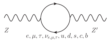
Figure 1: Cross terms between $Z$ and $Z^{\prime}$ particles.

Besides the self-energy of each particle, the self-energy among different types of particles, or the “cross terms” may also give rise to the imaginary parts, as shown in Fig. 1 as an example. This is not a problem if $Z$ and $Z^{\prime}$ are well separated in mass spectrum, and its contributions are suppressed by a factor $\frac{1}{m_{Z^{\prime}}^{2}-m_{Z}^{2}}$ so they can be taken into account order-by-order perturbatively. However, when $Z$ and $Z^{\prime}$ are nearly degenerate so $m_{Z^{\prime}}^{2}\approx m_{Z}^{2}$, such a suppression becomes non-viable.

Denote $c_{XY}\equiv\rm{Im}\left\{\Pi_{X\leftrightarrow Y}(p^{2}\approx m_{X,Y}^{2})\right\}$, where $\Pi_{X\leftrightarrow Y}(p^{2})$ is the $g_{\mu\nu}$ coefficient of the self-energy of a particle $X$ transforming into $Y$, one has to correct each element of (5) with an additional $ic_{XY}$ term before the diagonalizion processes. In fact, as we will illustrate in Appendix A, in order to keep the photon massless, we utilize the matrix below

$$\mathcal{M}_{V}^{2~{}\prime} = \mathcal{M}_{V}^{2}+i\left(C_{X\leftrightarrow Y}\right)_{3\times 3}$$ (8)

$$= \begin{pmatrix}m_{\hat{Z}^{\prime}}^{2}+ic_{\hat{Z}^{\prime}\hat{Z}^{\prime}}&\hat{g}^{\prime}(\delta m^{2}-\frac{ic_{\hat{Z}^{\prime}\hat{Z}}}{\sqrt{\hat{g}^{\prime 2}+\hat{g}^{2}}})&-\hat{g}(\delta m^{2}-\frac{ic_{\hat{Z}^{\prime}\hat{Z}}}{\sqrt{\hat{g}^{\prime 2}+\hat{g}^{2}}})\\ \hat{g}^{\prime}(\delta m^{2}-\frac{ic_{\hat{Z}^{\prime}\hat{Z}}}{\sqrt{\hat{g}^{\prime 2}+\hat{g}^{2}}})&\frac{\hat{g}^{\prime 2}}{4}(\hat{v}^{2}+\delta v^{2}+\frac{4ic_{\hat{Z}\hat{Z}}}{\hat{g}^{\prime 2}+\hat{g}^{2}})&-\frac{\hat{g}^{\prime}\hat{g}}{4}(\hat{v}^{2}+\delta v^{2}+\frac{4ic_{\hat{Z}\hat{Z}}}{\hat{g}^{\prime 2}+\hat{g}^{2}})\\ -\hat{g}(\delta m^{2}-\frac{ic_{\hat{Z}^{\prime}\hat{Z}}}{\sqrt{\hat{g}^{\prime 2}+\hat{g}^{2}}})&-\frac{\hat{g}^{\prime}\hat{g}}{4}(\hat{v}^{2}+\delta v^{2}+\frac{4ic_{\hat{Z}\hat{Z}}}{\hat{g}^{\prime 2}+\hat{g}^{2}})&\frac{\hat{g}^{2}}{4}(\hat{v}^{2}+\delta v^{2}+\frac{4ic_{\hat{Z}\hat{Z}}}{\hat{g}^{\prime 2}+\hat{g}^{2}})\end{pmatrix},$$

Now the mass terms are no longer hermitian, and this can be understood by adding some non-conjugate corrections into the Lagrangian, or the Hamiltonian, just as what happens in a $K^{0}$-$\overline{K^{0}}$ systemDonoghue:1992dd ; Workman:2022ynf . We also have to note that the “hatted” $\hat{Z}$ denotes the “SM-$\hat{Z}$” when all the mixing terms are switched off, that is to say,

$$\hat{Z}^{\mu}=\frac{1}{\sqrt{\hat{g}^{2}+\hat{g}^{\prime 2}}}(-\hat{g}^{\prime}B^{\mu}+\hat{g}W^{3\mu}).$$ (9)

In the following of this paper, the hatless “$Z$” usually appears within the symbols associated with the aspect of the experimentalists who might be unaware that their observed resonance can accommodate exotic contributions. “$Z$” also appears within the definitions from the literature or simulating tools. In this paper, the hatless “$Z^{\prime}$” is also associated with a general reference of “$Z^{\prime}$-model” or “$Z^{\prime}$-$Z$ system”, while the hatted “$\hat{Z^{\prime}}$” particularly refers to the $\hat{Z^{\prime}}$ field that we introduce in (1).

Then we can follow Ref. Cai:2022cti to diagonalize the kinetic matrix (7) beforehand:

$$V_{C}=V_{1}V_{2}V_{3},\quad V_{C}^{\mathrm{T}}\mathcal{K}_{V}V_{C}=I_{3\times 3},$$ (10)

where

$$V_{1} = \begin{pmatrix}1&-\epsilon_{B}&-\epsilon_{W}\\ 0&1&0\\ 0&0&1\end{pmatrix},~{}V_{2}=\begin{pmatrix}1&0&0\\ 0&1&\frac{-\epsilon_{BW}+\epsilon_{B}\epsilon_{W}}{1-\epsilon_{B}^{2}}\\ 0&0&1\end{pmatrix},$$

$$V_{3} = \begin{pmatrix}1&0&0\\ 0&\frac{1}{\sqrt{1-\epsilon_{B}^{2}}}&0\\ 0&0&\sqrt{\frac{1-\epsilon_{B}^{2}}{1+\epsilon_{WW}-\epsilon_{B}^{2}-\epsilon_{W}^{2}-\epsilon_{BW}^{2}-\epsilon_{B}^{2}\epsilon_{WW}+2\epsilon_{B}\epsilon_{W}\epsilon_{BW}}}\end{pmatrix},$$ (11)

and then the mass-squared matrix becomes

$$(V_{1}V_{2}V_{3})^{\mathrm{T}}\mathcal{M}_{V}^{2~{}\prime}V_{1}V_{2}V_{3},$$ (12)

and diagonalizing this matrix gives

$$V=V_{1}V_{2}V_{3}V_{\mathrm{SM}}V_{\mathrm{f}},\quad V^{\mathrm{T}}\mathcal{M}_{V}^{2~{}\prime}V=\mathrm{diag}(m^{2}_{1}-\mathrm{i}m_{1}\Gamma_{1},\,m_{2}^{2}-\mathrm{i}m_{2}\Gamma_{2},\,0),$$ (13)

where $V_{\mathrm{SM}}$ is the familiar EW rotation matrix

$$V_{\text{SM}}=\begin{pmatrix}1&0&0\\ 0&-\frac{\hat{g}^{\prime}}{\sqrt{\hat{g}^{\prime 2}+\hat{g}^{2}}}&\frac{\hat{g}}{\sqrt{\hat{g}^{\prime 2}+\hat{g}^{2}}}\\ 0&\frac{\hat{g}}{\sqrt{\hat{g}^{\prime 2}+\hat{g}^{2}}}&\frac{\hat{g}^{\prime}}{\sqrt{\hat{g}^{\prime 2}+\hat{g}^{2}}}\end{pmatrix}.$$ (14)

$m_{1}$, $\Gamma_{1}$, $m_{2}$, $\Gamma_{2}$ are the “masses” and “widths” of two “mass eigenstates” of the $Z^{\prime}$-$Z$ system. Since their masses are nearly degenerate, and their mixing angle might be large, they might altogether form a single SM-$Z$-like object, and which of them is identified to be the $Z$- or $Z^{\prime}$ is unessential.

We have to note that although (8) is no longer hermitian, one can still verify that it is symmetric, that is, $\mathcal{M}_{V}^{2~{}\prime}=(\mathcal{M}_{V}^{2~{}\prime})^{\rm{T}}$. This guarantees the existence of $V_{\mathrm{f}}$ in (13) with the condition $V_{\mathrm{f}}^{\mathrm{T}}V_{\mathrm{f}}=V_{\mathrm{f}}V_{\mathrm{f}}^{\mathrm{T}}=I$. However, the elements of $V_{\mathrm{f}}$ can be complex, which are weird to be understood as the “mixing terms” among real vector fields, since the mixed “eigenstate fields” are no longer real numbers. This indicates that the usual perceptions of the “mixing fields” are non-viable and should be replaced with the concept of the resummmed propagators as described in Appendix A.

III Details of the event generation and the extraction of the observables

The standard way to extract the electroweak precision data is to compare the line-shape of the $Z$-resonance with the parameterized functions considering the Breit-Wigner propagators, initial-state radiation (ISR) effects, and the momentum distribution of the beams (See section 55 of “Reviews, Tables & Plots” in Ref. Workman:2022ynf for a review, and for the references therein). The photon mediated s-channel diagrams and all the t- and u-channel contributions with the interference effects should also be considered. After finding out the most fitted parameterized function, $m_{Z}$, $\Gamma_{Z}$, $R_{e,\mu,\tau}$, $A_{\rm FB}^{0e,\mu,\tau}$, and $N_{\nu}$, which are the mass of the $Z$-boson, the width of the $Z$-boson, the ratios of the $Z\rightarrow\rm{hadrons}$ over $Z\rightarrow e/\mu/\tau$ branching ratios, the forward-backward asymmetry parameters, and the effective number of the active neutrinos, respectively, are extracted for further comparison with the SM predicted values.

In this paper, we alternatively adopt what we called the “SM templates” to replace the role of the parameterized functions. These are the line-shape data acquired from the event generator based upon the dubbed “pseudo-SM” model file, which is a modified variation of the default SM model file provided by FeynRulesAlloul:2013bka , added with four additional parameters $m_{Z}$, $s^{2}_{l}$, $\Gamma_{Z}$ and $\xi$ as the input value. Here $s^{2}_{l}$ is the effective Weinberg angle affecting the weak coupling constants, independent with the $s^{2}_{W}$ associated with the ratio of the $W$ and $Z$ bosons. $\Gamma_{Z}$ can also be assigned with an arbitrary value, which might not equal to the SM-predicted one. $\xi$ appears in

$$B_{\mu} = -s_{W}\xi Z_{\mu}+c_{W}A_{\mu},$$

$$W^{3}_{\mu} = c_{W}\xi Z_{\mu}+s_{W}A_{\mu},$$ (15)

modifying the definitions of the $B_{\mu}$ and $W^{3}_{\mu}$ in the model file. This parameter aims at rescaling the height of the resonance while keeping the shape of it intact.

The purpose to utilize the event generator to generate the “pseudo-SM templates” is to elude the complicated comparison between our generator results and the SM values with intricated loop-level contribution considered under various renormalization schemes. Since the real LEP data are absent, it is also reasonable to compare our simulated $Z^{\prime}$-model events with the SM templates generated by exactly the same event generator, eliminating the errors from the theoretical uncertainties automatically.

To compare the continuous line-shape curves, one should sample a set of discrete $\sqrt{s}$’s, which are defined as the invariant mass, or the total energy of the colliding $e^{+}e^{-}$ system. LEP published some of the early detailed data at each of the sampled $\sqrt{s}$, while later as the integrated luminosity accumulates, only the fitted results of the electroweak precision measurements were published. With these incomplete information recorded in Ref. LEP:2000pgt , we adopt $\sqrt{s}=[88.2,89.2,90.2,91.2,92.2,93.2,94.2]\rm{GeV}$ as our samples as a reference, and the integrated luminosity is set 300 $\mathrm{pb}^{-1}$ for each $\sqrt{s}$ of the $Z^{\prime}$-model events. Since in Ref. LEP:2000pgt , the total luminosity is 60 $\mathrm{pb}^{-1}$, we therefore multiply a $\sqrt{5}$ when evaluating the statistical uncertainties. We call our data with such settings the “pseudo-LEP” results, and believe that these can characterize the main features of the LEP in the case of incomplete data.

For the pseudo-SM templates, we generate $10^{7}$ events for each $\sqrt{s}=[88.2$, $89.2$, $90.2$, $91.2$, $92.2$, $93.2$, $94.2]\rm{GeV}$ sample with various input values of $m_{Z}$, $s_{l}^{2}$, $\Gamma_{Z}$, and $\xi$. Then we use the polynomial

$$\sigma_{t}^{\text{PSM}}(m_{Z},\Gamma_{Z},s_{l}^{2},\xi,\sqrt{s})=a_{0t}(\sqrt{s})+(m_{Z}-m_{Z0})^{2}a_{1t}(\sqrt{s})+(s_{l}^{2}-s_{l0}^{2})^{2}a_{2t}(\sqrt{s})+$$ (16)

$$(\Gamma_{Z}-\Gamma_{Z0})^{2}a_{3t}^{F/B}(\sqrt{s})+(\xi-\xi_{0})^{2}a_{4t}(\sqrt{s})+(m_{Z}-m_{Z0})(s_{l}^{2}-s_{l0}^{2})a_{5t}(\sqrt{s})+$$

$$(m_{Z}-m_{Z0})(\Gamma_{Z}-\Gamma_{Z0})a_{6t}(\sqrt{s})+(m_{Z}-m_{Z0})(\xi-\xi_{0})a_{7t}(\sqrt{s})+(s_{l}^{2}-s_{l0}^{2})(\Gamma_{Z}-\Gamma_{Z0})a_{8t}(\sqrt{s})$$

$$+(s_{l}^{2}-s_{l0}^{2})(\xi-\xi_{0})a_{9t}(\sqrt{s})+(\Gamma_{Z}-\Gamma_{Z0})(\xi-\xi_{0})a_{10t}(\sqrt{s})+(m_{Z}-m_{Z0})a_{11t}(\sqrt{s})+$$

$$(s_{l}^{2}-s_{l0}^{2})a_{12t}(\sqrt{s})+(\Gamma_{Z}-\Gamma_{Z0})a_{13t}(\sqrt{s})+(\xi-\xi_{0})a_{14t}(\sqrt{s}),$$

to fit the pseudo-SM template events by quadratic fitting for each $\sqrt{s}=[88.2$, $89.2$, $90.2$, $91.2$, $92.2$, $93.2$, $94.2]\rm{GeV}$ in each final product channel $t\in\{(e^{+}e^{-})_{\text{F}/\text{B}}$,$(\mu^{+}\mu^{-})_{\text{F}/\text{B}}$,$\rm{hadrons}\}$. Here the subscript of the “$(e^{+}e^{-})_{\text{F}}$” or “$(e^{+}e^{-})_{\text{B}}$” denotes the “forward” or “backward” directions that the positive charged product outcomes parallels or anti-parallels to the incoming positron beam. The $a_{(0-14)t}$ are the factors to be determined by the fitting processes. The charge asymmetry of the quarks also affect the charge unbalance of the final hadrons, however analyzing such an asymmetry is beyond our ability of simulation, so we evade taking this into account.

In principle the $e^{+}e^{-}\rightarrow\tau^{+}\tau^{-}$ channels should also be considered. $\tau$ might decay into muons, electrons, or hadrons to fake the corresponding channels. The leptonic decay channels can be distinguished by the additional missing energy/momentum criterion during the event selections, and the hadronic decay channels might be problematic. At a lepton collider, the hadronic $\tau$-decay products can be well discriminated from the hadronic-jet eventsGrunewald:1995ny . The efficiency of the “$\tau$-tagging” techniques at a hadronic collider seems to have been significantly improved during these yearsBagliesi:2007qx ; CMS:2018jrd , and it is reasonable to expect that such a technology might in turn contribute to the future lepton collider programs. However, all these algorithms are too complicated for a fast simulation in this paper, and with the consideration of the technology improvement in the future, we just assume that all the $\tau$ products can be well-discriminated, so we neglect them in this paper.

In this work, we apply WHIZARD Kilian:2007gr ; Moretti:2001zz ; Christensen:2010wz as our event generator. LHAPDF6 Buckley:2014ana ; Andersen:2014efa , PYTHIA6 Bierlich:2022pfr , FastJet Cacciari:2005hq ; Cacciari:2011ma and DELPHES deFavereau:2013fsa ; Selvaggi:2014mya ; Mertens:2015kba are connected for the detective-level data. In DELPHES, we utilize the CEPC card regardless our purpose for a LEP-like prediction, and not so many differences are expected. The beams structure is chosen to be the Gaussian distribution. The WHIZARD parameter $\sigma$ of both the “gaussian_spread1” and “gaussian_spread2” are set to be 250/90000. ISR is also switched on. During the event generation, the cuts are set $\mathrm{E}\geq 100$ MeV, all $\mathrm{abs}(\cos(\mathrm{Theta}))\geq 0.8$ and all $\mathrm{M2}\geq 1$ $\mathrm{GeV}^{2}$ for final products, where “E”, “Theta” and “M2” are energy of the particle in the argument, absolute polar angle in the lab frame and invariant mass squared of the particle in the argument, respectively. Then transverse momentum $\mathrm{P_{T}}>7$ GeV and pseudorapidity $\eta<2.4$ are set for event selection.

We then compare the line-shape cross sections in the $Z^{\prime}$-model for each parameter point with the pseudo-SM template cross sections fitted in (16) to find the best fitted $(m_{Z}^{*},s_{l}^{*2},\Gamma_{Z}^{*},\xi^{*})$ by minimizing the $\chi_{F}^{2}$ defined as

$$\chi_{F}^{2}(m_{Z},\Gamma_{Z},s_{l}^{2},\xi)=\sum_{t,\sqrt{s}}\frac{(\sigma_{t}^{Z^{\prime}}(\sqrt{s})-\sigma_{t}^{\mathrm{PSM}}(m_{Z},\Gamma_{Z},s_{l}^{2},\xi,\sqrt{s}))^{2}}{(\Delta_{t}^{Z^{\prime}}(\sqrt{s}))^{2}+(\Delta_{i}^{\mathrm{PSM}}(m_{Z},\Gamma_{Z},s_{l}^{2},\xi,\sqrt{s}))^{2}},$$ (17)

where $\sqrt{s}=[88.2$, $89.2$, $90.2$, $91.2$, $92.2$, $93.2$, $94.2]\rm{GeV}$, $\sigma_{t}^{\mathrm{PSM}}(m_{Z},\Gamma_{Z},s_{l}^{2},\xi,\sqrt{s})$ is defined in (16). $\sigma_{t}^{Z^{\prime}}(\sqrt{s})$ are line-shape sample cross sections for the $Z^{\prime}$-model with a particular set of parameters. $\Delta_{i}^{Z^{\prime}}$ and $\Delta_{i}^{\mathrm{PSM}}(m_{Z},\Gamma_{Z},s_{l}^{2},\xi,\sqrt{s})$ are the statistical uncertainties of the pseudo-SM template cross sections and the $Z^{\prime}$-model cross sections respectively. The statistical uncertainty $\Delta_{\rm X}$ for each cross section $\sigma_{\rm X}$ at channel $X$ is evaluated by

$$\Delta_{\rm X}=\frac{1}{\sqrt{n_{\rm X}}}\sigma_{\rm X},$$ (18)

where $n_{\rm X}$ is the number of events passing through all selection criterion. The total $\chi_{F}^{2}$ includes seven points of center-of-mass energy, three channels, and the leptonic channels are separated into forward-back parts, so the total degree of freedom is counted to be 35.

Then the best-fitted $(m_{Z}^{*},s_{l}^{*2},\Gamma_{Z}^{*},\xi^{*})$ will be converted into effective oblique parameters $\tilde{S}$, $\tilde{T}$, $\tilde{U}$, and $\delta\tilde{N}_{\nu}$, which are the effective Peskin-Takeuchi oblique parameters and the the effective deviation of the species of neutrinos respectively. Ref. Peskin:1990zt ; Peskin:1991sw derived the $S$, $T$, $U$ expressions depending on $m_{W},s_{l},\Gamma_{Z}$. Here we reverse these formulas as the definitions of the effective $\tilde{S}$, $\tilde{T}$, $\tilde{U}$ so that the constraints of $S$, $T$, $U$ in the literature can be straightforwardly cast here. One subtle thing is that in the usual electroweak precision measurement discussions, $m_{Z}$ is the input parameter, so $\delta m_{W}$ is given by

$$\delta m_{W}=-\frac{\alpha m_{W}^{\mathrm{SM}}}{4(c_{\mathrm{W}}^{2}-s_{\mathrm{W}}^{2})}(S-2c^{2}_{\mathrm{W}}T-\frac{c_{\mathrm{W}}^{2}-s_{\mathrm{W}}^{2}}{2s^{2}_{\mathrm{W}}}U),$$ (19)

where $\delta m_{W}=m_{W}-m_{W}^{\mathrm{SM}}$. However, in our pseudo model, $m_{Z}$ is no longer the “measured” $Z$ boson mass. The correction on $m_{W}$ is equivalent to a correction on $m_{Z}$ towards the opposite direction, so according to $m_{W}^{\mathrm{SM}}=m_{Z}c_{\mathrm{W}}$, $m_{W}=m_{Z}^{\mathrm{SM}}c_{\mathrm{W}}$ and Ref. Ciuchini:2013pca ; Fan:2014vta , we define $\tilde{S}$, $\tilde{T}$, $\tilde{U}$, as well as the deviation of the neutrino species number $\delta\tilde{N}_{\nu}$ by solving the following equations.

$$m_{Z}^{*}-m_{Z}^{\mathrm{SM}} = \frac{\alpha m_{Z}^{\mathrm{SM}}}{4(c_{\mathrm{W}}^{2}-s_{\mathrm{W}}^{2})}(\tilde{S}-2c^{2}_{\mathrm{W}}\tilde{T}-\frac{c_{\mathrm{W}}^{2}-s_{\mathrm{W}}^{2}}{2s^{2}_{\mathrm{W}}}\tilde{U}),$$

$$s_{l}^{*2}-(s_{l}^{2})^{\mathrm{SM}} = \frac{\alpha}{4(c_{\mathrm{W}}^{2}-s_{\mathrm{W}}^{2})}(\tilde{S}-4s_{\mathrm{W}}^{2}c_{\mathrm{W}}^{2}\tilde{T}),$$

$$\Gamma_{Z}^{*}-(\Gamma_{Z})^{\mathrm{SM}} = \frac{\alpha^{2}m_{Z}^{\mathrm{SM}}}{72s^{2}_{\mathrm{W}}c^{2}_{\mathrm{W}}(c_{\mathrm{W}}^{2}-s_{\mathrm{W}}^{2})}(-10(3-8s^{2}_{\mathrm{W}})\tilde{S}+(63-126s^{2}_{\mathrm{W}}-40s^{4}_{\mathrm{W}})\tilde{T}),$$

$$\delta\tilde{N}_{\nu} = \frac{\Gamma_{Z}^{*}-(\Gamma_{Z})^{\mathrm{pSM}}}{(\Gamma_{\nu\nu})^{\mathrm{pSM}}},$$ (20)

where $m_{Z}^{\text{SM}}$ is the $\hat{Z}$-mass encoded in the model file of the $Z^{\prime}$-model file if all the vector boson’s mixing terms are switched off. $(s_{l}^{2})^{\mathrm{SM}}$ and $(\Gamma_{Z})^{\mathrm{SM}}$ are also the calculated values of $s_{l}^{2}$ and $\Gamma_{Z}$ in this case. $(\Gamma_{Z})^{\mathrm{pSM}}$ and $(\Gamma_{\nu\nu})^{\mathrm{pSM}}$ are calculated according to the pseudo-SM model files with the best fitted $m_{Z}^{*}$, $s_{l}^{*2}$ and $\xi^{*}$ as the input parameter. Solving (20), we obtain

$$\tilde{S} =367.29\delta s_{l}^{2}+37.92\delta\Gamma_{Z},$$ (21)

$$\tilde{T} =132.35\delta s_{l}^{2}+52.94\delta\Gamma_{Z},$$

$$\tilde{U} =-2.62\delta m_{Z}+144.31\delta s_{l}^{2}-37.92\delta\Gamma_{Z},$$

where $\delta m_{Z}=m_{Z}^{*}-m_{Z}^{\mathrm{SM}}$, $\delta s_{l}^{2}=s_{l}^{*2}-(s_{l}^{2})^{\mathrm{SM}}$ and $\delta\Gamma_{Z}=\Gamma_{Z}^{*}-(\Gamma_{Z})^{\mathrm{SM}}$.

	Result	Correlation
$S$	$0.06\pm 0.1$	$1.00$
$T$	$0.11\pm 0.12$	$0.90$	$1.00$
$U$	$-0.02\pm 0.09$	$-0.57$	$-0.82$	$1.00$

Table 1: Global fit results of the oblique parameters $S$, $T$, and $U$ adopted from Ref. Lu:2022bgw .

The $\chi^{2}$ comparing the $\tilde{S}$, $\tilde{T}$ and $\tilde{U}$ with the global fitted data is defined by

$$\chi^{2}=\begin{pmatrix}\tilde{S}-S_{0},&\tilde{T}-T_{0},&\tilde{U}-U_{0}\end{pmatrix}C^{-1}\begin{pmatrix}\tilde{S}-S_{0}\\ \tilde{T}-T_{0}\\ \tilde{U}-U_{0}\end{pmatrix},$$ (22)

where $S_{0}$, $T_{0}$ and $U_{0}$ are the best global-fitted values, $C^{-1}$ represents the inverse of the covariance matrix of $S_{0}$, $T_{0}$ and $U_{0}$. In this paper, the $S_{0}$, $T_{0}$, $U_{0}$ and $C^{-1}$ are adopted from Tab. 1.

In this paper, based upon some typical models (See an enumeration of the $Z^{\prime}$-models in Ref. Langacker:2008yv , and the references therein), we are going to show our calculated $\tilde{S}$, $\tilde{T}$, $\tilde{U}$, $\delta\tilde{N}_{\nu}$, as well as the estimated $e^{+}e^{-}$ collider sensitivity in three scenarios. They are

• Scenario I: $\hat{Z}^{\prime}$ only couples to invisible particles.

  This scenario is inspired from the dark matter model associated with a $Z^{\prime}$, in which $Z^{\prime}$ plays a crucial role connecting the visible world with the dark sector. $Z^{\prime}$ might couple with the dark matter, and the dark matter particles decayed from it are invisible at a collider. Besides the dark matter, $Z^{\prime}$ might also couple with the sterile neutrino, which might also be invisible if they are long-lived enough to decay outside the detector.

  This scenario is accomplished by straightforwardly assigning a $c_{\hat{Z}^{\prime}\hat{Z}^{\prime}}$ value in (8) for convenience, rather than introducing some invisible fields for the $\hat{Z}^{\prime}$ to decay into them.

• Scenario II: $\hat{Z}^{\prime}$ couples with the SM fermions universally among all three generations.

  Charged under the $U(1)^{\prime}$ gauge symmetry universally among all three generations, the coupling constants are stringently constrained by the off-shell $\hat{Z}^{\prime}$ mediated processes, leading to a particularly small $c_{\hat{Z}^{\prime}\hat{Z}^{\prime}}$ to give a narrow but sharp valley-like structure imposed on the resonance. The initial momentum distribution in the beams and the ISR effect smear this structure to give a relatively “smooth” curve. Since the LEP collaborations only published the final electroweak precision measurement results, and they are acquired by comparing the experimental data with a trivial resonance structure, we only follow this principle to compare our pseudo-LEP results with the pseudo-SM templates to find the best-fitted electroweak observables, regardless of the non-standard resonance shape of the pseodu-LEP data.

  Here we define the coupling constants as

  $$g_{u_{R}}\hat{Z}^{\prime}_{\mu}\bar{u}_{R}\gamma^{\mu}u_{R}+g_{u_{L}}\hat{Z}^{\prime}_{\mu}\bar{u}_{L}\gamma^{\mu}u_{L} = \hat{Z}^{\prime}_{\mu}\bar{u}\gamma^{\mu}(\frac{g_{u_{L}}+g_{u_{R}}}{2}-\frac{g_{u_{L}}-g_{u_{R}}}{2}\gamma^{5})u,$$

  $$g_{d_{R}}\hat{Z}^{\prime}_{\mu}\bar{d}_{R}\gamma^{\mu}d_{R}+g_{d_{L}}\hat{Z}^{\prime}_{\mu}\bar{d}_{L}\gamma^{\mu}d_{L} = \hat{Z}^{\prime}_{\mu}\bar{d}\gamma^{\mu}(\frac{g_{d_{L}}+g_{d_{R}}}{2}-\frac{g_{d_{L}}-g_{d_{R}}}{2}\gamma^{5})u,$$

  $$g_{l_{R}}\hat{Z}^{\prime}_{\mu}\bar{l}_{R}\gamma^{\mu}l_{R}+g_{l_{L}}\hat{Z}^{\prime}_{\mu}\bar{l}_{L}\gamma^{\mu}l_{L} = \hat{Z}^{\prime}_{\mu}\bar{l}\gamma^{\mu}(\frac{g_{l_{L}}+g_{l_{R}}}{2}-\frac{g_{l_{L}}-g_{l_{R}}}{2}\gamma^{5})u,$$

  $$g_{\nu_{L}}\hat{Z}^{\prime}_{\mu}\bar{\nu}_{L}\gamma^{\mu}\nu_{L} = \hat{Z}^{\prime}_{\mu}\bar{\nu}(\frac{g_{\nu_{L}}}{2}-\frac{g_{\nu_{L}}}{2}\gamma^{5})\nu.$$ (23)

• Scenario III: $\hat{Z}^{\prime}$ couples with the SM fermions depending on their generations.

  For some particular models (Ref. Salvioni:2009jp enumerated such models, and references can be found therein), a particular generation of particles might be charged under the $U(1)^{\prime}$ group, or two generations of particles takes a particular combination of the $U(1)^{\prime}$ charge (For an example, the $U(1)_{L_{e}-L_{\mu}}$ modelsHe:1990pn ; He:1991qd ; Ma:2001md ; Foot:1994vd ; Baek:2001kca ). This not only affects the shape of the $Z$-resonance, but also breaks the universality of the $l^{+}l^{-}$ branching ratios, where $l=e,\mu,\tau$. In this paper, we only discuss the $e$-$\mu$ asymmetry, and utilize the

  $$\frac{R_{e}}{R_{\mu}}$$ (24)

  where

  $$R_{l}\equiv\frac{\Gamma_{\mathrm{had}}}{\Gamma_{l^{+}l^{-}}}$$ (25)

  to observe such an asymmetry.

IV Numerical Results

The effective Lagrangian (1) takes six parameters, $m_{Z^{\prime}}$, $\epsilon_{B}$, $\Lambda_{W}$, $\Lambda_{BW}$, $\Lambda_{WW}$, $\lambda_{BD}$, which are not convenient for a relatively intuitive presentation. Equivalently, $\epsilon_{B}$, $\epsilon_{W}$, $\epsilon_{BW}$, $\delta v^{2}$, $\delta m^{2}$ and $m_{\hat{Z}^{\prime}}$ appeared in (8) and (11) and can be treated as the free parameters for further discussions. Among them, $\epsilon_{B}$ and $\epsilon_{W}$ and $m_{\hat{Z}^{\prime}}$ are the most important. In fact, the $\delta v^{2}$, $\epsilon_{BW}$ have nothing to do with the $Z^{\prime}$ sector, so their contributions are perturbatively calculable by previous algorithms and we do not discuss them. $\delta m^{2}$ can also give rise to non-perturbative mixings, however in this paper, we focus on the kinematic mixing effects.

In the following of this section, we plot the $\tilde{S}$, $\tilde{T}$, $\tilde{U}$ and $\delta\tilde{N}_{\nu}$ for Scenario I-III on the continuous $\epsilon_{B}$-$\epsilon_{W}$ plain with some discrete $\delta m_{Z^{\prime}}=m_{Z^{\prime}}-m_{Z}^{\rm SM}$ values adopted. For Scenario III when universality among generations is broken, $\frac{\tilde{R}_{e}}{\tilde{R}_{\mu}}-1$ is also plotted. Here the definition of $m_{Z}^{\rm SM}$ is the same as in (20).

The Monte-Carlo algorithm that we utilize inevitably introduces statistical fluctuations in our results, thus smoothness is lost in the plotted figures. We use a second-order polynomial of $\epsilon_{B}$ and $\epsilon_{W}$ to fit each of the fluctuated $\tilde{S}$, $\tilde{T}$, $\tilde{U}$, $\delta\tilde{N}_{\nu}$ and $\frac{\tilde{R}_{e}}{\tilde{R}_{\mu}}-1$ by least square method to smooth the results. The constant terms of the second-order polynomials are set zero since all new physics corrections are destined to vanish at the $\epsilon_{B}=\epsilon_{W}=0$ origin. The similar results from several independent runs with different random seeds verify the reliability of this fitting algorithm, so in this paper, we show the fitted results in the figures.

In principle, we should compare our results with the global fitted results of all $\tilde{S}$, $\tilde{T}$, $\tilde{U}$, $\delta\tilde{N}_{\nu}$, and $\frac{\tilde{R}_{e}}{\tilde{R}_{\mu}}-1$ parameters. Unfortunately, in the literature $\tilde{S}$, $\tilde{T}$, $\tilde{U}$ are fitted with the assumption of universality and $\delta\tilde{N}_{\nu}=0$. $\delta\tilde{N}_{\nu}$ is also fitted with the assumption that the visible $Z$-propagator is not distorted, that is to say, $\tilde{S}=0$, $\tilde{T}=0$, $\tilde{U}=0$. A complete global fitting including all these parameters is far beyond our target, and remember that we are only able to show readers the “sensitivity” of a LEP-like electron-positron collider without performing a real fitting process due to the lack of the published data, so in this paper, we still show the corresponding “STU-$(1,2)$-$\sigma$”, “$\delta\tilde{N}_{\nu}$-$(1,2)$-$\sigma$”, “$R_{e}/R_{\mu}$-$(1,2)$-$\sigma$” contours in each of the figures. The prefixes “STU-”, “$\delta\tilde{N}_{\nu}$-”, “$R_{e}/R_{\mu}$-” indicate that the $1$-$\sigma$ and $2$-$\sigma$ fitted results originate from the global fitted oblique parameter in Tab. 1, indirect $N_{\nu}$ results from Ref. Workman:2022ynf , $R_{e}$ and $R_{\mu}$ data with their uncertainties adopted from Ref. Workman:2022ynf . However we should note that these contours only characterize the sensitivity of the collider on this model, and should not be regarded as real constraints.

Besides, people are more interested about the sensitivity of some proposed future colliders. According to Ref. CEPCStudyGroup:2018ghi , the CEPC is expected to significantly improve the uncertainties of the electroweak precision measurements. With the expected sensitivities published in Ref. CEPCStudyGroup:2018ghi around the $Z$-pole, we also plot the “CEPC-ST-$(1,2)$-$\sigma$”, “CEPC-$\delta\tilde{N}_{\nu}$-$(1,2)$-$\sigma$”, “CEPC-$R_{e}/R_{\mu}$-$(1,2)$-$\sigma$” contours within one plot for each of the $\epsilon_{B}$ and $\epsilon_{W}$ plain. Note that Ref. CEPCStudyGroup:2018ghi only shows the expected $S$-$T$ results in Figure 11.18, so we are forced to give up the $U$. Although in principle $U$-sensitivity can be extracted from the Tab. 11.16 of Ref. CEPCStudyGroup:2018ghi , however the complete covariance matrix is missing for a complete fitting. Since we only target at the collider’s potential sensitivity, neglecting the $U$ is expected not to affect the final results significantly. Another subtle thing is that Ref. CEPCStudyGroup:2018ghi only gives $R_{\mu}$, which is insufficient to estimate the $R_{e}/R_{\mu}$ uncertainties. In fact, at a lepton collider, the $e^{+}e^{-}\rightarrow e^{+}e^{-}$ channel data are slightly less precise than the corresponding $e^{+}e^{-}\rightarrow\mu^{+}\mu^{-}$ data because of the less accuracy of the electron/positron trajectory measurements. It is also reasonable to assume that the CEPC $R_{e}$ uncertainty decreases synchronously with the $R_{\mu}$ uncertainty as the integrated luminosity increases, so the $R_{e}$ uncertainty at CEPC can be reasonably estimated by assuming that the ratio of the $R_{e}$ and $R_{\mu}$ uncertainties should remain similar to the LEP results recorded in Ref. CEPCStudyGroup:2018ghi .

Now we show our results for the three scenarios respectively.

IV.1 Scenario I: $\hat{Z}^{\prime}$ couples with invisible matters

In this scenario, the width $\Gamma_{\hat{Z}^{\prime}}$ that $\hat{Z}^{\prime}$ only decays to invisible matter is regarded as a input parameter, so $c_{\hat{Z}^{\prime}\hat{Z}^{\prime}}$ and $c_{\hat{Z}\hat{Z}}$ are given by

$$c_{\hat{Z}^{\prime}\hat{Z}^{\prime}}=-m_{\hat{Z}^{\prime}}\Gamma_{\hat{Z}^{\prime}},\quad c_{\hat{Z}\hat{Z}}=-m_{Z}^{\mathrm{SM}}\Gamma_{Z}^{\mathrm{SM}},$$ (26)

Since the $\hat{Z}^{\prime}$ has no coupling to SM fermions, there is no self energy diagram of $\hat{Z}^{\prime}$-$\hat{Z}$. Therefore we have

$$c_{\hat{Z}^{\prime}\hat{Z}}=0.$$ (27)

If the $\Gamma_{\hat{Z}^{\prime}}$ is close to $\Gamma_{Z}^{\mathrm{SM}}$, and the $m_{\hat{Z}^{\prime}}$ is also close to $m_{Z}^{\mathrm{SM}}$, maximum mixings between $Z^{\prime}$-$Z$ might arise, however the overlapped and interfered peaks still look like a single $Z$-pole.

For convenience we define

$$\lambda_{Z^{\prime}}=\frac{\Gamma_{\hat{Z}^{\prime}}}{\Gamma_{Z}^{\mathrm{SM}}},$$ (28)

which is the ratio of the widths of the two “interaction-eigenstates”. We have tried several combinations of parameters like $\delta m_{Z^{\prime}}=0,-0.1$ GeV, and $\lambda_{Z^{\prime}}=0.5,0.9$, and found that the results are quite similar if $\hat{Z}^{\prime}$ and $\hat{Z}$ are nearly-degenerate. Therefore, we choose to plot the results when $\lambda_{Z^{\prime}}=0.9$ and $\delta m_{Z^{\prime}}=-0.1$ GeV in Fig. 2 as a paradigm.

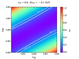
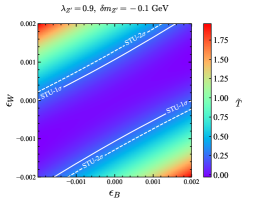
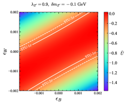
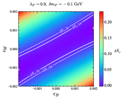
Figure 2: Plots for $\delta m_{Z^{\prime}}=-0.1$ GeV, $\lambda_{Z^{\prime}}=0.9$ and $\delta v^{2}=\epsilon_{WW}=\epsilon_{BW}=\delta m^{2}=0$ on the $\epsilon_{B}$-$\epsilon_{W}$ plain. The lower right panel shows the estimated CEPC sensitivity. The remaining four panels display the heat maps of $\tilde{S}$, $\tilde{T}$, $\tilde{U}$ and $\delta\tilde{N}_{\nu}$, and plot the 1-$\sigma$ and 2-$\sigma$ contours on the $\epsilon_{B}$-$\epsilon_{W}$ plain. Current $N_{\nu}$ data is extracted from Ref. Workman:2022ynf .

IV.2 Scenario II: $\hat{Z}^{\prime}$ couples with the SM fermions universally among all three generations

In this scenario, $\hat{Z}^{\prime}$ couples directly with the SM quarks and leptons. General definitions of the coupling constants have been listed in (23). To compute the $\text{Im}\Pi_{\hat{Z}^{\prime}\hat{Z}}$, the fermions’ couplings with the $\hat{Z}_{\mu}$ fields are required.

$$\mathcal{L}\supset\hat{Z}_{\mu}\bar{\psi}^{f}\gamma^{\mu}(V_{\hat{Z}}^{f}-A_{\hat{Z}}^{f}\gamma^{5})\psi^{f},\quad f=u,d,l,\nu$$ (29)

where according to the SM,

$$V_{\hat{Z}}^{u}=\frac{1}{4c_{\mathrm{W}}}-\frac{2s^{2}_{\mathrm{W}}}{3c_{\mathrm{W}}},\quad A_{\hat{Z}}^{u}=\frac{1}{4c_{\mathrm{W}}},\quad V_{\hat{Z}}^{d}=-\frac{1}{4c_{\mathrm{W}}}+\frac{s^{2}_{\mathrm{W}}}{3c_{\mathrm{W}}},\quad A_{\hat{Z}}^{d}=-\frac{1}{4c_{\mathrm{W}}},$$

$$V_{\hat{Z}}^{l}=-\frac{1}{4c_{\mathrm{W}}}+\frac{s^{2}_{\mathrm{W}}}{c_{\mathrm{W}}},\quad A_{\hat{Z}}^{l}=-\frac{1}{4c_{\mathrm{W}}},\quad V_{\hat{Z}}^{\nu}=\frac{1}{4c_{\mathrm{W}}},\quad A_{\hat{Z}}^{\nu}=\frac{1}{4c_{\mathrm{W}}}.$$ (30)

Denote $V_{\hat{Z}^{\prime}}^{f}\equiv\frac{g_{f_{L}}+g_{f_{R}}}{2}$ and $A_{\hat{Z}^{\prime}}^{f}\equiv\frac{g_{f_{L}}-g_{f_{R}}}{2}$, under the approximation that the decay products are massless, $c_{\hat{Z}\hat{Z}}$, $c_{\hat{Z}^{\prime}\hat{Z}}$ and $c_{\hat{Z}^{\prime}\hat{Z}^{\prime}}$ are calculated to be

$$c_{\hat{Z}\hat{Z}} = -m_{Z}^{\mathrm{SM}}\Gamma_{Z}^{\mathrm{SM}},$$

$$c_{\hat{Z}^{\prime}\hat{Z}^{\prime}} = -\frac{(m_{Z}^{\mathrm{SM}})^{2}}{12\pi}\sum_{f\neq t}(V^{f}_{\hat{Z}^{\prime}}V^{f}_{\hat{Z}^{\prime}}+A^{f}_{\hat{Z}^{\prime}}A^{f}_{\hat{Z}^{\prime}}),$$

$$c_{\hat{Z}^{\prime}\hat{Z}} = -\frac{(m_{Z}^{\mathrm{SM}})^{2}}{12\pi}\sum_{f\neq t}(V^{f}_{\hat{Z}^{\prime}}V^{f}_{\hat{Z}}+A^{f}_{\hat{Z}^{\prime}}A^{f}_{\hat{Z}}).$$ (31)

In this scenario, the direct coupling constants between $\hat{Z}^{\prime}$ and the SM particles should be stringently constrained. Therefore the $c_{\hat{Z}^{\prime}\hat{Z}^{\prime}}$ and $c_{\hat{Z}^{\prime}\hat{Z}}$ become much smaller than $c_{\hat{Z}\hat{Z}}$. This actually suppresses the mixing angle and in this case, the $\hat{Z}^{\prime}$-like object cleaves a deep but narrow valley within the resonance induced by the $Z$-like object, which will later be smeared by the ISR and beam momentum distribution effects, just as we have plotted in Fig. 3 as an example.

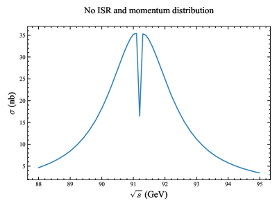
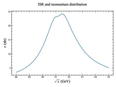
Figure 3: $Z$ line-shape predicted by an example model that $\hat{Z}^{\prime}$ couples with the SM fermions. The left panel shows the results when the electron/positron is “bare”, while the right panel considers the ISR and beam momentum distribution effects.

It is actually impossible for a practical lepton collider to scan every $\sqrt{s}$ in a sufficient resolution to depict such inconspicuous structure, so what we can do is still adopt the scattered $\sqrt{s}=[88.2$, $89.2$, $90.2$, $91.2$, $92.2$, $93.2$, $94.2]\rm{GeV}$ samples to extract the $\tilde{S}$, $\tilde{T}$, $\tilde{U}$, $\delta\tilde{N}_{\nu}$ parameters.

In this paper, we only consider two cases, one is that the $\hat{Z}^{\prime}$ only couples universally with all the leptons, and the other is that the $\hat{Z}^{\prime}$ couple with leptons and quarks with the ratio of the coupling constants to be $3:1$, inspired by the $U(1)_{B-L}$ model. For the first case, since we find out that the chirality of the interaction terms defined in (23) does not affect the results to a significant extent, we only adopt the vector-type interaction pattern $g_{l_{L}}=g_{l_{R}}$, and show an example when $g_{l_{L}}=g_{l_{R}}=0.001$ in Fig. 4. Inspired by the $U(1)_{B-L}$ models, we plot the Fig. 5 as an example when $g_{l_{L}}=g_{l_{R}}=-3g_{u_{L}}=-3g_{u_{R}}=-3g_{d_{L}}=-3g_{d_{R}}=0.0015$. One can again evaluate the LEP sensitivity as well as the estimated CEPC sensitivity on the $\epsilon_{B}$-$\epsilon_{W}$ plain.

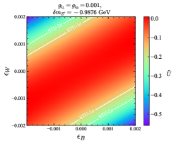
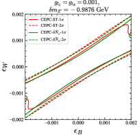
Figure 4: Plots for $\hat{m}_{Z^{\prime}}=90.2$ GeV, $g_{l_{L}}=g_{l_{R}}=0.001$ and $\delta v^{2}=\epsilon_{WW}=\epsilon_{BW}=\delta m^{2}=g_{u_{L}}=g_{u_{R}}=g_{d_{L}}=g_{d_{R}}=g_{\nu_{L}}=0$ on the $\epsilon_{B}$-$\epsilon_{W}$ plain. The other symbols are the same as in Fig. 2.

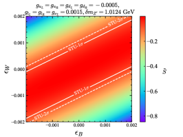
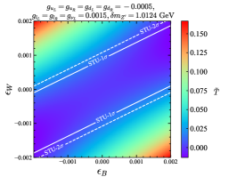
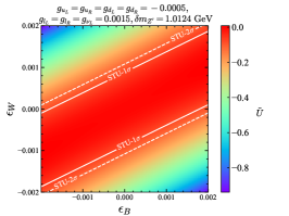
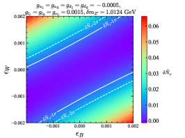
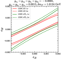
Figure 5: Plots for $\hat{m}_{Z^{\prime}}=92.2$ GeV, $g_{u_{L}}=g_{u_{R}}=g_{d_{L}}=g_{d_{R}}=-0.0005$, $g_{l_{L}}=g_{l_{R}}=g_{\nu_{L}}=0.0015$ and $\delta v^{2}=\epsilon_{WW}=\epsilon_{BW}=\delta m^{2}=0$ on the $\epsilon_{B}$-$\epsilon_{W}$ plain. The other symbols are the same as in Fig. 2

IV.3 Scenario III: $\hat{Z}^{\prime}$ couples with the SM fermions depending on the generations

The $Z^{\prime}$ couplings to fermions might be generation-dependent, in which case coefficients in (23) need to be changed into the generation-dependent version. Constrained by our current calculation ability and inspired by some eminent models, we only consider the case that $\hat{Z}^{\prime}$ only couples with $\mu$ and/or $\tau$. The interaction terms are parametrized by

$$\mathcal{L}_{\mathrm{eff}}\supset\hat{Z}^{\prime}_{\mu}\bar{\mu}\gamma^{\mu}(\frac{g_{\mu_{L}}+g_{\mu_{R}}}{2}-\frac{g_{\mu_{L}}-g_{\mu_{R}}}{2})\mu+\hat{Z}^{\prime}_{\mu}\bar{\tau}\gamma^{\mu}(\frac{g_{\tau_{L}}+g_{\tau_{R}}}{2}-\frac{g_{\tau_{L}}-g_{\tau_{R}}}{2})\tau.$$ (32)

Since $e^{+}e^{-}\rightarrow\mu^{+}\mu^{-}$ might be affected by (32), firstly, we delete the all the $\mu^{+}\mu^{-}$ terms in (17) to find the best-fitted point in our pseudo-SM template, then again $\tilde{S}$, $\tilde{T}$, $\tilde{U}$, $\delta\tilde{N}_{\nu}$ are extracted.

To translate the definition in (24) into the expression of our simulated data, we adopt

$$\frac{R_{e}}{R_{\mu}}=\frac{\sigma^{\mathrm{NP}}_{\mu^{+}\mu^{-}}(\sqrt{s}=m_{Z})}{\sigma^{\mathrm{NP}}_{se^{+}e^{-}}(\sqrt{s}=m_{Z})},$$ (33)

where subscript “$s$” in $\sigma^{\mathrm{NP}}_{se^{+}e^{-}}(m_{Z})$ indicates the $s$-channel cross section the $e^{+}e^{-}\rightarrow e^{+}e^{-}$ channel. Certainly, $\sigma^{\mathrm{NP}}_{se^{+}e^{-}}(m_{Z})$ is impossible to acquire straightforwardly due to the contamination from the $t$-, $u$-channels. Fortunately, in the pseudo-SM template, the universality is preserved, and the $\sigma^{\mathrm{PSM}}_{\mu^{+}\mu^{-}}$ does not include the $t$-, $u$-channel contributions. Therefore, the $\sigma^{\mathrm{PSM}}_{\mu^{+}\mu^{-}}(\sqrt{s}=91.2~{}\mathrm{GeV})$ adopted from the pseudo-SM template can be utilized in place of $\sigma^{\mathrm{NP}}_{se^{+}e^{-}}(m_{Z})$, and we also take $\sqrt{s}=91.2\rm{GeV}$ to replace the $m_{Z}$, so

$$\frac{R_{e}}{R_{\mu}}=\frac{\sigma^{\mathrm{NP}}_{\mu^{+}\mu^{-}}(\sqrt{s}=91.2~{}\mathrm{GeV})}{\sigma^{\mathrm{PSM}}_{\mu^{+}\mu^{-}}(\sqrt{s}=91.2~{}\mathrm{GeV})}.$$ (34)

We will extract the current $\frac{R_{e}}{R_{\mu}}$ data from Ref. Workman:2022ynf , and plot the $1$-$\sigma$ and $2$-$\sigma$ contour in the $\epsilon_{B}$-$\epsilon_{W}$ plain. The CEPC sensitivity is extracted from Ref. CEPCStudyGroup:2018ghi . Notice that according to Ref. CEPCStudyGroup:2018ghi , the sensitivity of “$R_{l}$” denoted there is actually $R_{\mu}$. Usually the detector’s sensitivities on electron/positrons are a bit lower than those on muons, and it is reasonable to expect the uncertainties of $R_{e}$ and $R_{\mu}$ at the same collider will synchronously decrease as the integrated luminosity rises. Therefore, we estimate the expected uncertainty of the $R_{e}$ at CEPC by multiplying the expected uncertainty of the $R_{\mu}$ by the same factor of the ratio of the uncertainties of $R_{e}$ and $R_{\mu}$ recorded in Ref. Workman:2022ynf . Therefore, the expected uncertainty of $\frac{R_{e}}{R_{\mu}}$ at CEPC can be extracted.

Inspired by the models that $Z^{\prime}$ couples with a particular generation of leptons, we show an example that the $\hat{Z}^{\prime}$ only couples with the second family of the leptons in Fig. 6. Inspired by the $U(1)_{L_{e}-L_{\mu}}$ modelsHe:1990pn ; He:1991qd ; Ma:2001md ; Foot:1994vd ; Baek:2001kca , we show an example in Fig. 7.

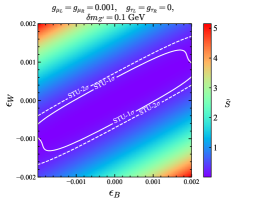
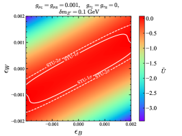
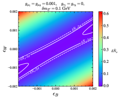
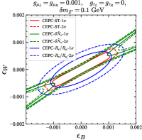
Figure 6: Plots for $\delta m_{Z^{\prime}}=0.1$ GeV, $g_{\mu_{L}}=g_{\mu_{R}}=0.001$ and $g_{\tau_{L}}=g_{\tau_{R}}=\delta v^{2}=\epsilon_{WW}=\epsilon_{BW}=\delta m^{2}=0$ on the $\epsilon_{B}$-$\epsilon_{W}$ plain. Compared with the Fig. 2, $\frac{R_{e}}{R_{\mu}}-1$ is additionally plotted.

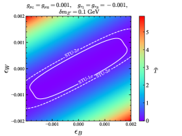
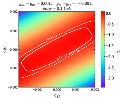
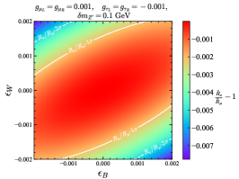
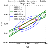
Figure 7: Plots for $\delta m_{Z^{\prime}}=0.1$ GeV, $g_{\mu_{L}}=g_{\mu_{R}}=0.001$, $g_{\tau_{L}}=g_{\tau_{R}}=-0.001$ and $\delta v^{2}=\epsilon_{WW}=\epsilon_{BW}=\delta m^{2}=0$ on the $\epsilon_{B}$-$\epsilon_{W}$ plain. The other symbols are the same as in Fig. 6

V Summary

In a nearly-degenerate $Z^{\prime}$-$Z$ system, not only the widths, or equivalently, the imaginary part of the self-energy diagram of each fields, but also the indispensable “cross terms”, that is to say, the imaginary part of the self-energy diagram connecting two different fields play important roles in calculating the line-shape observables. After diagonalizing the “mass matrix” with the imaginary contributions included, sometimes “SM-like $Z$” and “$Z^{\prime}$” cannot be well discriminated and they overlap coherently to form a single resonance-like object which might be recognized as a single particle.

Relying on the effective field theory model in which many of the $Z^{\prime}$ models can be accommodated, we simulate the shape of this resonance-like object, and follow the usual literature to utilize “oblique parameters” $\tilde{S}$, $\tilde{T}$, $\tilde{U}$, and “neutrino species deviation” $\delta\tilde{N}_{\nu}$ to describe the shape of it. Comparing the results with the current data mainly contributed by the LEP, one can estimate the sensitivity of the LEP at the $\epsilon_{B}$ and $\epsilon_{W}$ plain if the LEP data can be reanalyzed. As a paradigm of the future high-luminosity lepton colliders, the predicted sensitivity of this model at the CEPC is also evaluated. Besides, we also estimate the $R_{e}/R_{\mu}-1$ of the non-universality models, and compare them with the LEP and CEPC sensitivities.

Appendix A Resummation of the imaginary parts of the self-energy diagrams

Let us start from a group of real scalar particles for simplicity, e.g., $\phi_{i}$, $i=1,2,\dots,n$, with the mass matrix to be $\mathcal{M}^{2}_{s}=\{m^{2}_{ij}\}$ where $m^{2}_{ij}=m^{2}_{ji}$ so $\mathcal{M}_{s}^{2T}=\mathcal{M}_{s}^{2}$, and the mass terms being $\mathcal{L}_{m}=-\frac{1}{2}\phi_{i}m^{2}_{ij}\phi_{j}$. The complete propagator of these scalar particles can be written in the form of a matrix

$$\frac{i}{p^{2}I_{n\times n}-\mathcal{M}^{2}_{s}}\equiv i(p^{2}I_{n\times n}-\mathcal{M}^{2}_{s})^{-1}.$$ (35)

The usual diagonalization processes to find the mass eigenstates of $\phi_{i}$’s are equivalent to finding an orthogonal matrix $V$ to diagonalize the propagator

$$iV(p^{2}I_{n\times n}-\mathcal{M}^{2}_{s})^{-1}V^{-1}=\text{diag}\left[\frac{i}{p^{2}-m_{1}^{2}},\frac{i}{p^{2}-m_{2}^{2}},\dots,\frac{i}{p^{2}-m_{n}^{2}}\right],$$ (36)

where $V$ is a real matrix to satisfy $VV^{T}=V^{T}V=I$. Expand the left-hand side of (36) according to $\mathcal{M}^{2}_{s}$, we acquire

$$iV(p^{2}I_{n\times n}-\mathcal{M}^{2}_{s})^{-1}V^{-1}=iV\frac{1}{p^{2}}\left(I-\sum_{t=1}^{n}(\frac{\mathcal{M}^{2}_{s}}{p^{2}})^{n}\right)V^{-1}$$ (37)

$$= i\frac{1}{p^{2}}\left[I+\sum_{t=1}^{n}\left(\frac{V\mathcal{M}^{2}_{s}V^{-1}}{p^{2}}\right)^{n}\right]=i\left(p^{2}I_{n\times n}-V\mathcal{M}_{s}^{2}V^{-1}\right)^{-1}.$$

It is then clear to see that $\mathcal{M}_{s}^{2}$ and the propagator (36) must be diagonalized at the same time.

Including all the imaginary parts of the $\phi_{i}$-$\phi_{j}$ self-energy diagrams introduces a resummation

$$\sum_{t=0}^{\infty}\frac{i}{p^{2}I_{n\times n}-\mathcal{M}^{2}_{s}}\left[(-i)\text{Im}(\Sigma(p^{2}))\frac{i}{p^{2}I_{n\times n}-\mathcal{M}^{2}_{s}}\right]^{t}=\frac{i}{p^{2}I_{n\times n}-\mathcal{M}^{2}_{s}-\text{Im}(\Pi(p^{2}))},$$ (38)

where $-i\Pi(p^{2})$ is a $n\times n$ symmetric matrix with each of its element $-i\Pi_{jk}(p^{2})$ the (cross) self-energy diagram connecting $\phi_{j}$ and $\phi_{k}$. Therefore, a complete diagonalization process described in (37) should be replaced by

$$iV(p^{2}I_{n\times n}-\mathcal{M}^{2}_{s}-\text{Im}(\Pi(p^{2})))^{-1}V^{-1}=i\left\{p^{2}I_{n\times n}-V[\mathcal{M}_{s}^{2}+\text{Im}(\Pi(p^{2}))]V^{-1}\right\}^{-1}.$$ (39)

It is now clear that for the complete diagonalization processes including all the width informations, one should in turn diagonalize $\mathcal{M}_{s}^{2}+\text{Im}(\Pi(p^{2}))$ at each momentum $p$ instead of a mere $\mathcal{M}_{s}^{2}$. Again, it is easy to verify that $\mathcal{M}_{s}^{2}+\text{Im}(\Pi(p^{2}))$ is a complex symmetric diagram, which guarantees the possibility of a successful diagonalization by a complex orthogonal diagram $V=(V^{T})^{-1}$.

If all the scalars are nearly-degenerate around the mass $m_{d}$, a good approximation can be $p^{2}=m_{d}^{2}$ to preserve the accuracy of the near-shell performances of the propagators. This is a generalization of the Breig-Wigner propagator for the single particle into a nearly-degenerate multiple particle group.

Since we are discussing about the real scalars, and usually the complex orthogonal $V$ contains not only real numbers, if we treat $V$ as the matrix to recombine $\phi_{1,2,\dots,n}$ into “mass eigenstates” $\phi^{\prime}_{j}=V_{jk}\phi_{k}$ as usual, then $\phi^{\prime}_{j}$ is something “complex” but cannot be regarded as a “complex scalar field”. Therefore, in this paper, we remind the reader that (39) cannot be understood as a equivalence to diagonalizing the scalar fields, although we sometimes still apply this less rigorous terminology for brevity.

For the $W^{3}$-$B$-$Z^{\prime}$ system, the propagators should be accompanied with a Lorentz term

$$\frac{ig_{\mu\nu}}{p^{2}I_{3\times 3}-\mathcal{M}^{2}_{V}}\equiv ig_{\mu\nu}(p^{2}I_{3\times 3}-\mathcal{M}^{2}_{V})^{-1}.$$ (40)

Here we adopt the Feynmann gauge. In principle Goldstone propagators should also be considered. However, around the $Z$-pole, only light leptons and quarks can be produced on-shell. Even the heaviest $b$ quark takes the $m_{B}\sim 3$-$5$ GeV mass, so the Goldstone/Higgs contributions are suppressed by a $\left(\frac{m_{b}}{v}\right)^{2}\ll 1$ factor, and can be safely neglected.

Due to the Lorentz covariance, The one-loop self-energy diagram of the vector bosons can be decomposed and parametrized by

$$i\Pi^{\mu\nu}_{3\times 3}(p^{2})=i\Pi_{3\times 3}(p^{2})g^{\mu\nu}+i\Pi^{\prime}_{3\times 3}(p^{2})p^{\mu}p^{\nu}.$$ (41)

Then we can follow (38) to resum the vector boson’s propagators. Notice that all the masses of our initial and final state particles are ignorable since they are extremely relativistic particles, so once a $p^{\mu}$ in (41) appears, it will finally dots into the fermionic propagators of the external legs. The Ward-Takahashi identity version in the broken phaseChanowitz:1985hj transmute this into a Goldstone propagator, and its contributions are again suppressed by the smallness of the Yukawa couplings. Therefore, we are able to neglect the $p^{\mu}p^{\nu}$ terms in (41), and finally write down the resummed propagators when only imaginary parts of the (41) are considered

$$ig^{\mu\nu}\left[p^{2}I_{3\times 3}-\mathcal{M}^{2}_{v}-\text{Im}(\Pi_{3\times 3}(p^{2}))\right]^{-1}.$$ (42)

In principle, $\text{Im}(\Pi_{3\times 3}(p^{2}))$ should be computed for each $p$. However, practical event generators are not designed for such kind of propagators. If we just fix $p^{2}\approx m_{Z}^{\text{SM}2}$ in (42), the off-shell $s$-channel photon decay contributions are included, however the softer $t$-channel photon propagators might also become massive. To avoid the massive photon, we tentatively shut down the mixing terms, and diagonalize the

$$\mathcal{M}_{V}^{\text{SM}2} = \begin{pmatrix}m_{\hat{Z}^{\prime}}^{2}&0&0\\ 0&\frac{\hat{g}^{\prime 2}}{4}\hat{v}^{2}&-\frac{\hat{g}^{\prime}\hat{g}}{4}\hat{v}^{2}\\ 0&-\frac{\hat{g}^{\prime}\hat{g}}{4}\hat{v}^{2}&\frac{\hat{g}^{2}}{4}\hat{v}^{2}\end{pmatrix}.$$ (43)

Shutting down the mixing terms does not affect the self-energy calculations up to the one-loop order. Diagonalizing (43) requires $V_{\rm SM}$ defined in (14). $V_{\rm SM}^{T}\mathcal{M}_{V}^{\text{SM}2}V_{\rm SM}$ gives

$$\text{diag}[m_{\hat{Z}^{\prime}}^{2},m_{\hat{Z}}^{2},0],$$ (44)

corresponding to the masses of the “$\hat{Z}^{\prime}$”, “SM-like $\hat{Z}$” with the “hat” symbols to distinguish them from the true SM mass-eigenstates, and the photon “eigenstate” masses respectively. Here $m_{\hat{Z}^{\prime}}^{2}=\frac{\hat{g}^{2}+\hat{g}^{\prime 2}}{4}\hat{v}^{2}$. Actually, it is the $\hat{Z}^{\prime}$ and $\hat{Z}$ that are nearly degenerate and might strongly mix together, and the photon lies far from the $\hat{Z}^{\prime}$-$\hat{Z}$ mass spectrum, so we only have to consider $\Pi_{\hat{Z}\hat{Z}}(p^{2})$, $\Pi_{\hat{Z}^{\prime}\hat{Z}^{\prime}}(p^{2})$ and $\Pi_{\hat{Z}^{\prime}\hat{Z}}(p^{2})$, whose contributions are not able to be perturbatively expanded. With the definition $c_{XY}\equiv\rm{Im}\left\{\Pi_{X\leftrightarrow Y}(p^{2}\approx m_{X,Y}^{2})\right\}$, (44) becomes

$$V_{\rm SM}^{T}\mathcal{M}_{V}^{\text{SM}2}V_{\rm SM}+iC_{\hat{Z}/\hat{Z}^{\prime}}=\begin{pmatrix}m_{\hat{Z}^{\prime}}^{2}+ic_{\hat{Z}^{\prime}\hat{Z}^{\prime}}&ic_{\hat{Z}^{\prime}\hat{Z}}&0\\ ic_{\hat{Z}^{\prime}\hat{Z}}&m_{\hat{Z}}^{2}+ic_{\hat{Z}\hat{Z}}&0\\ 0&0&0\end{pmatrix}.$$ (45)

where $iC_{\hat{Z}/\hat{Z}^{\prime}}$ indicates the corrections from the imaginary parts of the self-energy diagrams. Then we utilize $V_{\rm SM}^{-1}=V_{\rm SM}^{T}$ to restore (45) into the form under the “interacting eigenstate basis”,

$$V_{\rm SM}(V_{\rm SM}^{T}\mathcal{M}_{V}^{\text{SM}2}V_{\rm SM}+iC_{\hat{Z}/\hat{Z}^{\prime}})V_{\rm SM}^{T}$$ (46)

$$= \begin{pmatrix}m_{\hat{Z}^{\prime}}^{2}+ic_{\hat{Z}^{\prime}\hat{Z}^{\prime}}&-i\frac{\hat{g}^{\prime}}{\sqrt{\hat{g}^{\prime 2}+\hat{g}^{2}}}c_{\hat{Z}^{\prime}\hat{Z}}&i\frac{\hat{g}}{\sqrt{\hat{g}^{\prime 2}+\hat{g}^{2}}}c_{\hat{Z}^{\prime}\hat{Z}}\\ -i\frac{\hat{g}^{\prime}}{\sqrt{\hat{g}^{\prime 2}+\hat{g}^{2}}}c_{\hat{Z}^{\prime}\hat{Z}}&\frac{\hat{g}^{\prime 2}}{4}\left(\hat{v}^{2}+\frac{4ic_{\hat{Z}\hat{Z}}}{\hat{g}^{\prime 2}+\hat{g}^{2}}\right)&-\frac{\hat{g}^{\prime}\hat{g}}{4}\left(\hat{v}^{2}+\frac{4ic_{\hat{Z}\hat{Z}}}{\hat{g}^{\prime 2}+\hat{g}^{2}}\right)\\ i\frac{\hat{g}}{\sqrt{\hat{g}^{\prime 2}+\hat{g}^{2}}}c_{\hat{Z}^{\prime}\hat{Z}}&-\frac{\hat{g}^{\prime}\hat{g}}{4}\left(\hat{v}^{2}+\frac{4ic_{\hat{Z}\hat{Z}}}{\hat{g}^{\prime 2}+\hat{g}^{2}}\right)&\frac{\hat{g}^{2}}{4}\left(\hat{v}^{2}+\frac{4ic_{\hat{Z}\hat{Z}}}{\hat{g}^{\prime 2}+\hat{g}^{2}}\right)\end{pmatrix}.$$

Supplement (46) with the mixing terms $\delta m^{2}$, $\delta v^{2}$ appeared in (5), (8) is then acquired.

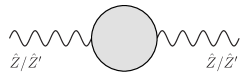
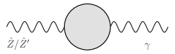
Figure 8: (Cross) self-energy terms connecting among $\tilde{Z}^{\prime}$, $\tilde{Z}$ and photon fields.

As we have mentioned, we include the imaginary parts of the diagrams in the first panel of Fig. 8, while neglecting the rest of them with the photon external leg(s) involved. Since the mass of the photon is far from the nearly-denegerate $Z^{\prime}$-$Z$ system, one find it possible to manipulate these photon-involved terms perturbatively in (45) and (46), in contrast with the non-perturbative $\hat{Z}$-$\hat{Z}^{\prime}$ mixing terms. Neglecting the photon-involved terms gives the error of $\sim\left[\frac{{\rm Im}\left(\Pi_{\gamma\hat{Z}^{(\prime)}}\right)}{m_{\hat{Z}}^{2}}\right]^{2}$, which can be ignored in our current stage of theoretical discussions.

In the practical event simulation processes that we have performed, we at first shut down all the mixing terms to calculate the width of the SM-Z boson by the event generator to extract the $c_{\hat{Z}\hat{Z}}$ from it. Then, we compute $c_{\hat{Z}^{\prime}\hat{Z}}$ and $c_{\hat{Z}^{\prime}\hat{Z}^{\prime}}$ by hand relying on different model setups. After diagonalizing (8) by our own programs, we acquire the “masses” and “widths” of the “mass eigenstates”, as well as the rotated “coupling constants” to be input into the event generator for further simulations, which is equivalent to diagonalizing the propagator matrix (42) to calculate the amplitudes.

References

- (1) P. Fayet, “Effects of the Spin 1 Partner of the Goldstino (Gravitino) on Neutral Current Phenomenology,” Phys. Lett. B 95 (1980) 285–289.
- (2) P. Fayet, “On the Search for a New Spin 1 Boson,” Nucl. Phys. B 187 (1981) 184–204.
- (3) L. B. Okun, “LIMITS OF ELECTRODYNAMICS: PARAPHOTONS?,” Sov. Phys. JETP 56 (1982) 502.
- (4) P. Fayet, “Extra U(1)’s and New Forces,” Nucl. Phys. B 347 (1990) 743–768.
- (5) B. Holdom, “Two U(1)’s and Epsilon Charge Shifts,” Phys. Lett. B 166 (1986) 196–198.
- (6) P. Galison and A. Manohar, “TWO Z’s OR NOT TWO Z’s?,” Phys. Lett. B 136 (1984) 279–283.
- (7) R. Foot and X.-G. He, “Comment on Z Z-prime mixing in extended gauge theories,” Phys. Lett. B 267 (1991) 509–512.
- (8) A. Leike, “The Phenomenology of extra neutral gauge bosons,” Phys. Rept. 317 (1999) 143–250, arXiv:hep-ph/9805494.
- (9) D0 Collaboration, V. M. Abazov et al., “Search for a Heavy Neutral Gauge Boson in the Dielectron Channel with 5.4 of Collisions at = 1.96 TeV,” Phys. Lett. B 695 (2011) 88–94, arXiv:1008.2023 [hep-ex].
- (10) CDF Collaboration, T. Aaltonen et al., “Search for High Mass Resonances Decaying to Muon Pairs in TeV Collisions,” Phys. Rev. Lett. 106 (2011) 121801, arXiv:1101.4578 [hep-ex].
- (11) CDF Collaboration, A. Abulencia et al., “Search for high-mass resonances decaying to e mu in collisions at 1.96-TeV.,” Phys. Rev. Lett. 96 (2006) 211802, arXiv:hep-ex/0603006.
- (12) CDF Collaboration, D. Acosta et al., “Search for new physics using high mass tau pairs from 1.96 TeV collisions,” Phys. Rev. Lett. 95 (2005) 131801, arXiv:hep-ex/0506034.
- (13) CDF Collaboration, T. Aaltonen et al., “A Search for resonant production of pairs in of integrated luminosity of collisions at ” Phys. Rev. D 84 (2011) 072004, arXiv:1107.5063 [hep-ex].
- (14) CDF Collaboration, T. Aaltonen et al., “Search for new particles decaying into dijets in proton-antiproton collisions at s**(1/2) = 1.96-TeV,” Phys. Rev. D 79 (2009) 112002, arXiv:0812.4036 [hep-ex].
- (15) CDF Collaboration, T. Aaltonen et al., “Search for and Resonances Decaying to Electron, Missing , and Two Jets in Collisions at TeV,” Phys. Rev. Lett. 104 (2010) 241801, arXiv:1004.4946 [hep-ex].
- (16) ATLAS Collaboration, G. Aad et al., “Search for high-mass dilepton resonances using 139 fb-1 of collision data collected at 13 TeV with the ATLAS detector,” Phys. Lett. B 796 (2019) 68–87, arXiv:1903.06248 [hep-ex].
- (17) CMS Collaboration, A. M. Sirunyan et al., “Search for resonant and nonresonant new phenomena in high-mass dilepton final states at = 13 TeV,” JHEP 07 (2021) 208, arXiv:2103.02708 [hep-ex].
- (18) CMS Collaboration, A. M. Sirunyan et al., “Search for a Narrow Resonance Lighter than 200 GeV Decaying to a Pair of Muons in Proton-Proton Collisions at TeV,” Phys. Rev. Lett. 124 no. 13, (2020) 131802, arXiv:1912.04776 [hep-ex].
- (19) LHCb Collaboration, R. Aaij et al., “Searches for low-mass dimuon resonances,” JHEP 10 (2020) 156, arXiv:2007.03923 [hep-ex].
- (20) ATLAS Collaboration, G. Aad et al., “Search for heavy Higgs bosons decaying into two tau leptons with the ATLAS detector using collisions at TeV,” Phys. Rev. Lett. 125 no. 5, (2020) 051801, arXiv:2002.12223 [hep-ex].
- (21) CMS Collaboration, A. M. Sirunyan et al., “Search for additional neutral MSSM Higgs bosons in the final state in proton-proton collisions at 13 TeV,” JHEP 09 (2018) 007, arXiv:1803.06553 [hep-ex].
- (22) ATLAS Collaboration, G. Aad et al., “Search for new resonances in mass distributions of jet pairs using 139 fb-1 of collisions at TeV with the ATLAS detector,” JHEP 03 (2020) 145, arXiv:1910.08447 [hep-ex].
- (23) CMS Collaboration, “Search for heavy resonances decaying to b quarks in proton-proton collisions at sqrt s=13 TeV,”.
- (24) ATLAS Collaboration, G. Aad et al., “Search for heavy particles in the -tagged dijet mass distribution with additional -tagged jets in proton-proton collisions at = 13 TeV with the ATLAS experiment,” Phys. Rev. D 105 no. 1, (2022) 012001, arXiv:2108.09059 [hep-ex].
- (25) M. E. Peskin and T. Takeuchi, “A New constraint on a strongly interacting Higgs sector,” Phys. Rev. Lett. 65 (1990) 964–967.
- (26) M. E. Peskin and T. Takeuchi, “Estimation of oblique electroweak corrections,” Phys. Rev. D 46 (1992) 381–409.
- (27) R. Barbieri, A. Pomarol, R. Rattazzi, and A. Strumia, “Electroweak symmetry breaking after LEP-1 and LEP-2,” Nucl. Phys. B 703 (2004) 127–146, arXiv:hep-ph/0405040.
- (28) B. Holdom, “Oblique electroweak corrections and an extra gauge boson,” Phys. Lett. B 259 (1991) 329–334.
- (29) K. S. Babu, C. F. Kolda, and J. March-Russell, “Implications of generalized Z - Z-prime mixing,” Phys. Rev. D 57 (1998) 6788–6792, arXiv:hep-ph/9710441.
- (30) G. Altarelli, R. Casalbuoni, F. Feruglio, and R. Gatto, “Bounds on extended gauge models from LEP data,” Phys. Lett. B 245 (1990) 669–680.
- (31) F. Richard, “Present and future sensitivity to a Z-prime,” 3, 2003. arXiv:hep-ph/0303107.
- (32) M. E. Peskin and J. D. Wells, “How can a heavy Higgs boson be consistent with the precision electroweak measurements?,” Phys. Rev. D 64 (2001) 093003, arXiv:hep-ph/0101342.
- (33) CDF Collaboration, T. Aaltonen et al., “High-precision measurement of the boson mass with the CDF II detector,” Science 376 no. 6589, (2022) 170–176.
- (34) A. Strumia, “Interpreting electroweak precision data including the W-mass CDF anomaly,” JHEP 08 (2022) 248, arXiv:2204.04191 [hep-ph].
- (35) P. Asadi, C. Cesarotti, K. Fraser, S. Homiller, and A. Parikh, “Oblique Lessons from the Mass Measurement at CDF II,” arXiv:2204.05283 [hep-ph].
- (36) J. Fan, L. Li, T. Liu, and K.-F. Lyu, “W-boson mass, electroweak precision tests, and SMEFT,” Phys. Rev. D 106 no. 7, (2022) 073010, arXiv:2204.04805 [hep-ph].
- (37) J. Gu, Z. Liu, T. Ma, and J. Shu, “Speculations on the W-mass measurement at CDF*,” Chin. Phys. C 46 no. 12, (2022) 123107, arXiv:2204.05296 [hep-ph].
- (38) C.-T. Lu, L. Wu, Y. Wu, and B. Zhu, “Electroweak precision fit and new physics in light of the W boson mass,” Phys. Rev. D 106 no. 3, (2022) 035034, arXiv:2204.03796 [hep-ph].
- (39) J. de Blas, M. Pierini, L. Reina, and L. Silvestrini, “Impact of the Recent Measurements of the Top-Quark and W-Boson Masses on Electroweak Precision Fits,” Phys. Rev. Lett. 129 no. 27, (2022) 271801, arXiv:2204.04204 [hep-ph].
- (40) K.-Y. Zhang and W.-Z. Feng, “Explaining the W boson mass anomaly and dark matter with a U(1) dark sector*,” Chin. Phys. C 47 no. 2, (2023) 023107, arXiv:2204.08067 [hep-ph].
- (41) Y.-P. Zeng, C. Cai, Y.-H. Su, and H.-H. Zhang, “Z boson mixing and the mass of the W boson,” Phys. Rev. D 107 no. 5, (2023) 056004, arXiv:2204.09487 [hep-ph].
- (42) A. W. Thomas and X. G. Wang, “Constraints on the dark photon from parity violation and the W mass,” Phys. Rev. D 106 no. 5, (2022) 056017, arXiv:2205.01911 [hep-ph].
- (43) Y. Cheng, X.-G. He, F. Huang, J. Sun, and Z.-P. Xing, “Dark photon kinetic mixing effects for the CDF W-mass measurement,” Phys. Rev. D 106 no. 5, (2022) 055011, arXiv:2204.10156 [hep-ph].
- (44) C. Cai, D. Qiu, Y.-L. Tang, Z.-H. Yu, and H.-H. Zhang, “Corrections to electroweak precision observables from mixings of an exotic vector boson in light of the CDF W-mass anomaly,” Phys. Rev. D 106 no. 9, (2022) 095003, arXiv:2204.11570 [hep-ph].
- (45) M. Algueró, J. Matias, A. Crivellin, and C. A. Manzari, “Unified explanation of the anomalies in semileptonic B decays and the W mass,” Phys. Rev. D 106 no. 3, (2022) 033005, arXiv:2201.08170 [hep-ph].
- (46) M. Du, Z. Liu, and P. Nath, “CDF W mass anomaly with a Stueckelberg-Higgs portal,” Phys. Lett. B 834 (2022) 137454, arXiv:2204.09024 [hep-ph].
- (47) K. Harigaya, E. Petrosky, and A. Pierce, “Precision Electroweak Tensions and a Dark Photon,” arXiv:2307.13045 [hep-ph].
- (48) J. F. Donoghue, E. Golowich, and B. R. Holstein, Dynamics of the Standard Model : Second edition, vol. 2. Oxford University Press, 2014.
- (49) Particle Data Group Collaboration, R. L. Workman and Others, “Review of Particle Physics,” PTEP 2022 (2022) 083C01.
- (50) ALEPH, DELPHI, L3, OPAL, SLD, LEP Electroweak Working Group, SLD Electroweak Group, SLD Heavy Flavour Group Collaboration, S. Schael et al., “Precision electroweak measurements on the resonance,” Phys. Rept. 427 (2006) 257–454, arXiv:hep-ex/0509008.
- (51) ILC Collaboration, “The International Linear Collider Technical Design Report - Volume 2: Physics,” arXiv:1306.6352 [hep-ph].
- (52) CEPC Study Group Collaboration, M. Dong et al., “CEPC Conceptual Design Report: Volume 2 - Physics & Detector,” arXiv:1811.10545 [hep-ex].
- (53) FCC Collaboration, A. Abada et al., “FCC-ee: The Lepton Collider: Future Circular Collider Conceptual Design Report Volume 2,” Eur. Phys. J. ST 228 no. 2, (2019) 261–623.
- (54) X.-C. Zheng, C.-H. Chang, and T.-F. Feng, “A proposal on complementary determination of the effective electro-weak mixing angles via doubly heavy-flavored hadron production at a super Z-factory,” Sci. China Phys. Mech. Astron. 63 no. 8, (2020) 281011, arXiv:1810.09393 [hep-ph].
- (55) A. Alloul, N. D. Christensen, C. Degrande, C. Duhr, and B. Fuks, “FeynRules 2.0 - A complete toolbox for tree-level phenomenology,” Comput. Phys. Commun. 185 (2014) 2250–2300, arXiv:1310.1921 [hep-ph].
- (56) LEP, ALEPH, DELPHI, L3, OPAL, Line Shape Sub-Group of the LEP Electroweak Working Group Collaboration, “Combination procedure for the precise determination of Z boson parameters from results of the LEP experiments,” arXiv:hep-ex/0101027.
- (57) M. W. Grunewald, “Tau physics at LEP,” Phys. Scripta 53 (1996) 257–290.
- (58) G. Bagliesi, “Tau tagging at Atlas and CMS,” in 17th Symposium on Hadron Collider Physics 2006 (HCP 2006). 7, 2007. arXiv:0707.0928 [hep-ex].
- (59) CMS Collaboration, A. M. Sirunyan et al., “Performance of reconstruction and identification of leptons decaying to hadrons and in pp collisions at 13 TeV,” JINST 13 no. 10, (2018) P10005, arXiv:1809.02816 [hep-ex].
- (60) W. Kilian, T. Ohl, and J. Reuter, “WHIZARD: Simulating Multi-Particle Processes at LHC and ILC,” Eur. Phys. J. C 71 (2011) 1742, arXiv:0708.4233 [hep-ph].
- (61) M. Moretti, T. Ohl, and J. Reuter, “O’Mega: An Optimizing matrix element generator,” arXiv:hep-ph/0102195.
- (62) N. D. Christensen, C. Duhr, B. Fuks, J. Reuter, and C. Speckner, “Introducing an interface between WHIZARD and FeynRules,” Eur. Phys. J. C 72 (2012) 1990, arXiv:1010.3251 [hep-ph].
- (63) A. Buckley, J. Ferrando, S. Lloyd, K. Nordström, B. Page, M. Rüfenacht, M. Schönherr, and G. Watt, “LHAPDF6: parton density access in the LHC precision era,” Eur. Phys. J. C 75 (2015) 132, arXiv:1412.7420 [hep-ph].
- (64) J. R. Andersen et al., “Les Houches 2013: Physics at TeV Colliders: Standard Model Working Group Report,” arXiv:1405.1067 [hep-ph].
- (65) C. Bierlich et al., “A comprehensive guide to the physics and usage of PYTHIA 8.3” arXiv:2203.11601 [hep-ph].
- (66) M. Cacciari and G. P. Salam, “Dispelling the myth for the jet-finder,” Phys. Lett. B 641 (2006) 57–61, arXiv:hep-ph/0512210.
- (67) M. Cacciari, G. P. Salam, and G. Soyez, “FastJet User Manual,” Eur. Phys. J. C 72 (2012) 1896, arXiv:1111.6097 [hep-ph].
- (68) DELPHES 3 Collaboration, J. de Favereau, C. Delaere, P. Demin, A. Giammanco, V. Lemaître, A. Mertens, and M. Selvaggi, “DELPHES 3, A modular framework for fast simulation of a generic collider experiment,” JHEP 02 (2014) 057, arXiv:1307.6346 [hep-ex].
- (69) M. Selvaggi, “DELPHES 3: A modular framework for fast-simulation of generic collider experiments,” J. Phys. Conf. Ser. 523 (2014) 012033.
- (70) A. Mertens, “New features in Delphes 3,” J. Phys. Conf. Ser. 608 no. 1, (2015) 012045.
- (71) M. Ciuchini, E. Franco, S. Mishima, and L. Silvestrini, “Electroweak Precision Observables, New Physics and the Nature of a 126 GeV Higgs Boson,” JHEP 08 (2013) 106, arXiv:1306.4644 [hep-ph].
- (72) J. Fan, M. Reece, and L.-T. Wang, “Possible Futures of Electroweak Precision: ILC, FCC-ee, and CEPC,” JHEP 09 (2015) 196, arXiv:1411.1054 [hep-ph].
- (73) P. Langacker, “The Physics of Heavy Gauge Bosons,” Rev. Mod. Phys. 81 (2009) 1199–1228, arXiv:0801.1345 [hep-ph].
- (74) E. Salvioni, A. Strumia, G. Villadoro, and F. Zwirner, “Non-universal minimal Z’ models: present bounds and early LHC reach,” JHEP 03 (2010) 010, arXiv:0911.1450 [hep-ph].
- (75) X. G. He, G. C. Joshi, H. Lew, and R. R. Volkas, “NEW Z-prime PHENOMENOLOGY,” Phys. Rev. D 43 (1991) 22–24.
- (76) X.-G. He, G. C. Joshi, H. Lew, and R. R. Volkas, “Simplest Z-prime model,” Phys. Rev. D 44 (1991) 2118–2132.
- (77) E. Ma, D. P. Roy, and S. Roy, “Gauged L(mu) - L(tau) with large muon anomalous magnetic moment and the bimaximal mixing of neutrinos,” Phys. Lett. B 525 (2002) 101–106, arXiv:hep-ph/0110146.
- (78) R. Foot, X. G. He, H. Lew, and R. R. Volkas, “Model for a light Z-prime boson,” Phys. Rev. D 50 (1994) 4571–4580, arXiv:hep-ph/9401250.
- (79) S. Baek, N. G. Deshpande, X. G. He, and P. Ko, “Muon anomalous g-2 and gauged L(muon) - L(tau) models,” Phys. Rev. D 64 (2001) 055006, arXiv:hep-ph/0104141.
- (80) M. S. Chanowitz and M. K. Gaillard, “The TeV Physics of Strongly Interacting W’s and Z’s,” Nucl. Phys. B 261 (1985) 379–431.