Agent Coordination via Contextual Regression (AgentCONCUR) for Data Center Flexibility

Abstract

A network of spatially distributed data centers can provide operational flexibility to power systems by shifting computing tasks among electrically remote locations. However, harnessing this flexibility in real-time through the standard optimization techniques is challenged by the need for sensitive operational datasets and substantial computational resources. To alleviate the data and computational requirements, this paper introduces a coordination mechanism based on contextual regression. This mechanism, abbreviated as AgentCONCUR, associates cost-optimal task shifts with public and trusted contextual data (e.g., real-time prices) and uses regression on this data as a coordination policy. Notably, regression-based coordination does not learn the optimal coordination actions from a labeled dataset. Instead, it exploits the optimization structure of the coordination problem to ensure feasible and cost-effective actions. A NYISO-based study reveals large coordination gains and the optimal features for the successful regression-based coordination.

I Introduction

Coordinated operations of bulk power systems and coupled infrastructures allow for leveraging their complementarity and offsetting inefficiencies, thus leading to enhanced performance. Coordination schemes synchronize grid operations with distribution [1], natural gas [2], and district heating [3] systems, and more recently, a large coordination potential has emerged from the networks of data centers (NetDC) [4]. Their unique coordination advantage is in spatial flexibility, which distributed data centers provide by shifting computing tasks among electrically remote locations. This flexibility resource will be important for future power grids, as electricity demand of data centers is rapidly growing, and is expected to reach 35 GW by 2030 in the U.S. alone [5]. Even at present, the coordination potential is significant: training a single GPT-3 language model – the core of the popular ChatGPT chatbot – consumes as much as 1.3 GWh [6]. Allocating such energy-intensive tasks in the NetDC is thus likely to predetermine the dispatch cost and emission intensity in adjacent grids.

The growing environmental footprint of computing has encouraged large internet companies to optimize NetDC operations in a carbon-aware manner. Using online emission monitoring tools, such as WattTime.org and ElectricityMaps.com, they smartly time and allocate computing tasks in regions with the least emission footprint [7, 8]. However, the sole reliance on limited emission data is the form of grid-agnostic coordination, which respects NetDC constraints yet ignores those of power grids. For grid-aware coordination, the literature offers three coordination mechanisms: demand response [4], enhanced market design [9], and co-optimization of grid and NetDC operations [10]. In practice, participation of data centers in demand response is very limited due to performance concerns [4]. While the second mechanism integrates the spatial flexibility within market-clearing algorithms and even features robust market properties [11], it remains challenging to fully represent complex data center objectives (e.g., quality of service) and constraints (e.g., latency) via single utility function. The latter co-optimization mechanism models the ideal power-NetDC coordination with the potential for the full representation of operational constraints, akin to coordination models for conventional energy infrastructures [1]–[3]. However, large data requirements and short operational time frames hinder such coordination in practice.

This paper develops a new, regression-based mechanism for grid-aware coordination of power systems and NetDC, termed AgentCONCUR. Unlike optimization-based coordination, the regression solely acts on available contextual grid information, while approximating the optimal decision-making of the two systems. As such, AgentCONCUR resembles industry practices in [7] and [8] by relying on limited grid data, while also leveraging the optimization structure of the ideal coordination. Specifically, this paper contributes by:

1) Developing a bilevel co-optimization of the power grid and NetDC operations, where power system decision-making is constrained by that of NetDC. Similar to grid-aware models in [9]–[11], this model takes the power system perspective, but it represents the NetDC as a separate, optimization problem with customer-oriented objectives and constraints (e.g., latency). This co-optimization provides the ideal solution.

2) Devising a contextual regression policy that efficiently approximates the ideal coordination. The policy feasibility and cost-consistency is ensured by the new training optimization which inherits the ideal optimization structure. Using sufficiently many operational scenarios in training allows for robust and cost-consistent performance across testing scenarios. Furthermore, the proposed training allows for the optimal coordination feature selection, such that the coordination can be made possible at different data-intensity requirements.

3) Performing a case study on the New York ISO system to estimate the cost-saving potential in the peak-hour coordination and its approximation by AgentCONCUR. Our results reveal practical trade-offs between the amount of contextual information (features) and the efficiency of coordination.

This paper also contributes to decision-focused learning. While the prior work focused on contextual data predictions, e.g., demand [12] or wind power generation [13] data, here we contextually predict the coordination decisions instead.

In the remainder, Section II details decision-making of power grid and NetDC operators, and then presents the ideal coordination. Section III introduces the contextual regression approach for AgentCONCUR. Section IV applies AgentCONCUR to New York ISO system and Section V concludes.

Notation: Lower- and upper-case letters denote vectors and matrices, respectively. For some matrix $A$, $a_{ij}$ denotes its element at position $(i,j)$. Symbol ^⊤ stands for transposition, and ^⋆ denotes the optimal value. Vectors $\mathbb{0}$ and $\mathbb{1}$ are of zeros and ones, respectively. Operator $\langle\cdot\rangle_{\text{F}}$ is the Frobenius inner product, and $\lVert\cdot\rVert_{p}$ denotes the $p-$norm.

II Optimizing Power and NetDC Coordination

Figure 1: Interfaces and notation of the power system, network of data centers (NetDC), and communication network between data centers and users.

We consider the power-NetDC coordination problem, where agents interface as pictured in Fig. 1. The NetDC operator chooses the spatial allocation of computing tasks among data centers, where the tasks come from a spatially distributed population of users. The allocation criterion is the minimum of network latency – a time delay between sending, executing and sending back the result of a computational task for all users. The resulting task allocation shapes electricity demand, which is then used in the optimal power flow (OPF) problem for power system dispatch. The two problems can thus be solved in a coordinated manner to minimize the dispatch cost.

The coordination is performed by means of spatial shifts of computing tasks using virtual links connecting data centers into a network [9]. These shifts must be coordinated to satisfy both power system and NetDC objectives. To enable such coordination, we formulate the following bilevel optimization, where the power system operator acts as a leader, whose decision space is constrained by the NetDC operator, acting as a follower:

$${\color[rgb]{1,1,1}.}\;\;\;\!\underset{{x,\varphi}}{\text{minimize}}\quad c_{\text{opf}}(x) {\scriptstyle\triangleright\texttt{ OPF cost}}$$

subject to $$x\in\mathcal{X}_{\text{opf}}(y) {\scriptstyle\triangleright\texttt{ OPF feasibility}}$$

$$\underset{{y}}{\text{minimize}}\quad c_{\text{net-dc}}(y) {\scriptstyle\triangleright\texttt{ Latency loss}}$$

$$\text{subject to}\quad\!y\in\mathcal{Y}_{\text{net-dc}}(\varphi)\quad {\scriptstyle\triangleright\texttt{ NetDC feasibility}}$$

where the task shift $\varphi$ is the coordination variable. The lower-level problem takes request $\varphi$ as input, and minimizes the latency loss by selecting the new task allocation $y$. The optimized allocation then enters the power flow equations, and the power system operators computes the new dispatch $x$ which minimizes the cost. The optimal solution $\varphi^{\star}$ achieves cost-optimal and feasible for the two systems coordination.

The rest of this section details decision-making of the two systems, and then presents the bilevel coordination problem.

II-A Power System Optimization

The operational setting builds on the standard DC-OPF problem [14], which computes the least-cost generation dispatch $p\in\mathbb{R}^{b}$, within limits $\underline{p},\overline{p}\in\mathbb{R}_{+}^{b}$, that satisfies electricity net demand – load $d\in\mathbb{R}_{+}^{b}$ subtracted by non-dispatchable renewable generation $r\in\mathbb{R}_{+}^{b}$. The dispatch cost is modeled using a quadratic function with the first- and second-order coefficients $c\in\mathbb{R}_{+}^{b}$ and $C\in\mathbb{S}_{+}^{b}$, respectively. The power flows are computed using the matrix of power transfer distribution factors $F\in\mathbb{R}^{b\times l}$, and must respect the line capacity $\overline{f}\in\mathbb{R}_{+}^{l}$. In rare cases, when generation lacks to satisfy all loads, we model load shedding $\ell\in\mathbb{R}^{b}$ with the most expensive cost $s\gg c$. In this notation, the OPF problem is:

$$\underset{{p,\ell}}{\text{minimize}}\quad c^{\top}p+p^{\top}Cp+s^{\top}\ell$$ (1a)

subject to $$\mathbb{1}^{\top}\!(p+r+\ell-d-\Gamma\vartheta)=0,$$ (1b)

$$|F(p+r+\ell-d-\Gamma\vartheta)|\leqslant\overline{f},$$ (1c)

$$\underline{p}\leqslant p\leqslant\overline{p},\;\mathbb{0}\leqslant\ell\leqslant d,$$ (1d)

which minimizes the total dispatch cost (1a) subject to the power balance equation (1b), minimum and maximum power flow, generation, and load shedding limits in (1c)–(1d), respectively. Modelling Power–NetDC coordination, we distinguish between conventional loads $d$ and power consumption by data centers $\Gamma\vartheta$ in constraints (1b) and (1c), where auxiliary matrix $\Gamma\in\mathbb{R}^{b\times n}$ converts computing loads $\vartheta\in\mathbb{R}^{n}$ of $n$ data centers into electrical loads. Although restrictive, this linear conversion model is consistent with power consumption models under different utilization regimes of data centers [15].

II-B NetDC Optimization

The NetDC operator allocates computing tasks of $m$ users among $n$ data centers. For some computing demand $\delta\in\mathbb{R}^{m}$, allocation $W\in\mathbb{R}^{n\times m}$ is optimized to satisfy conservation conditions $\vartheta_{i}=\sum_{j=1}^{m}w_{ij}$ and $\delta_{j}=\sum_{i=1}^{n}w_{ij}$, enforced for each data center $i$ and user $j$, respectively. The goal is to minimize the latency, which is proportional to geodesic distance $G\in\mathbb{R}^{n\times m}$ between users and data centers [16]. The proxy function for the aggregated latency is then defined as

$$\mathcal{L}:\mathbb{R}^{n\times m}\mapsto\mathbb{R},\quad\mathcal{L}(W)=\sum_{i=1}^{n}\sum_{j=1}^{m}g_{ij}w_{ij}.$$ (2)

The optimal task allocation problem then becomes:

$$\underset{{W,\vartheta\geqslant\mathbb{0}}}{\text{minimize}}\quad \mathcal{L}(W)+\varrho\lVert W\rVert_{2}^{2}$$ (3a)

subject to $$W^{\top}\mathbb{1}=\delta,$$ (3b)

$$W\mathbb{1}=\vartheta,$$ (3c)

which minimizes latency subject to task conservation conditions (3b) and (3c). The objective function (3a) additionally includes a quadratic term that evenly allocates tasks among equally remote data centers, using a small parameter $\varrho>0$.

Although the data center loading $\vartheta^{\star}$ is latency-optimal, it is ignorant of the processes in the power system and may shape an expensive electricity demand allocation $\Gamma\vartheta^{\star}$. In this case, consider a task shift request $\varphi\in\mathbb{R}^{k}$ along $k=\frac{n(n-1)}{2}$ virtual links available in a fully connected NetDC. Also, consider the incidence matrix $A\in\mathbb{R}^{n\times k}$ of the directed NetDC, where

$$a_{ij}=\left\{\!\!\begin{array}[]{rl}+1,&\text{if}\;i=n\\ -1,&\text{if}\;i=n^{\prime}\end{array}\right.\quad\forall j=(n,n^{\prime})\in 1,\dots,k.$$

Then, given some nominal solution $W^{\star},\vartheta^{\star}$ from (3), and some exogenous task shift request $\varphi$, the tasks are re-allocated in a latency-aware fashion by solving the following optimization:

$$\underset{{W,\vartheta\geqslant\mathbb{0}}}{\text{minimize}}\quad \tfrac{1}{2}\lVert\mathcal{L}(W-W^{\star})\rVert_{2}^{2}$$ (4a)

subject to $$W^{\top}\mathbb{1}=\delta,$$ (4b)

$$W\mathbb{1}=\vartheta,$$ (4c)

$$A\varphi=\vartheta-\vartheta^{\star},$$ (4d)

$$\mathcal{L}(W-W^{\star})\leqslant\alpha\mathcal{L}(W^{\star}).$$ (4e)

The problem seeks a new task allocation $W$ that deviates the least from the latency-optimal solution $W^{\star}$. Indeed, the objective function (4a) minimizes the latency loss, subject to the task conservation requirements (4b)–(4c). Equation (4d) re-distributes the nominal loading $\vartheta^{\star}$ with respect to exogenous task shift $\varphi$. The last constraint (4e) ensures that the aggregated latency must not exceed an $\alpha-$percentage of the nominal latency. Thus, problem (4) does not permit task shifts $\varphi$ that increase the network latency beyond the allowable amount.

II-C Bilevel Optimization for Power and NetDC Coordination

Since the vector of spatial task shifts $\varphi$ affects the OPF costs in (1) and the latency optimality loss in (4) simultaneously, $\varphi$ is modeled as a coordination variable between power system and NetDC operators. The cost-optimal and feasible task shift is found by solving the following bilevel optimization:

$$\begin{array}[]{@{}rl@{}}\underset{{p,\ell,\varphi}}{\text{minimize}}&c^{\top}p+p^{\top}Cp+s^{\top}\ell\\ \text{subject to}&\mathbb{1}^{\top}\!(p+r+\ell-d-\Gamma\vartheta)=0,\\ &|F(p+r+\ell-d-\Gamma\vartheta)|\leqslant\overline{f},\\ &\underline{p}\leqslant p\leqslant\overline{p},\;\mathbb{0}\leqslant\ell\leqslant d,\end{array}$$ (BL.U)

$$\quad\quad\quad\!\begin{array}[]{@{}rll}\vartheta\in\underset{W,\vartheta}{\text{argmin}}\!\!\!\!&\tfrac{1}{2}\lVert\mathcal{L}(W-W^{\star})\rVert_{2}^{2}&\\ \text{subject to}\!\!\!\!&W^{\top}\mathbb{1}=\delta,&\!\!\!\!\!:\mu\\ &W\mathbb{1}=\vartheta,&\!\!\!\!\!:\nu\\ &A\varphi=\vartheta-\vartheta^{\star},&\!\!\!\!\!:\kappa\\ &w_{ij}\geqslant 0,\;\;\!\!\forall i,j,&\!\!\!\!\!:\omega\\ &\mathcal{L}(W-W^{\star})\leqslant\alpha\mathcal{L}(W^{\star}),&\!\!\!\!\!:\gamma\end{array}$$ (BL.L)

which identifies the cost-optimal task shift $\varphi$ in (BL.U), anticipating the response of NetDC in (BL.L) in terms of new data center loading $\vartheta$. Here, the colon signs define the dual variables associated with each constraint in (BL.L). The common solution strategy for this problem is to replace (BL.L) with its Karush–Kuhn–Tucker (KKT) conditions [17], yielding a mixed-integer formulation detailed in Appendix -A.

III Agent Coordination via Contextual Regression (AgentCONCUR)

Solving the bilevel program (BL) in real-time is challenging because of large data requirements, the lack of coordination interfaces between the power grid and NetDC operators, and the computational burden of the bilevel problem that may fail to provide the solution within operational time frames. To bypass these coordination challenges, we adopt a contextual regression approach, which consists of two stages. At the first (planning) stage, a regression policy is optimized to associate the cost-optimal tasks shifts with the contextual, easy-to-access in real-time information. At the second (real-time) stage, a trained regression policy instantly maps the contextual information into task shifts. The contextual information includes partial yet strongly correlated with grid conditions data, such as aggregated load and generation statistics, electricity prices correlated with costs, and power flows correlated with bus injections. Such contextual information is available online from many power system operators worldwide, e.g., [18].

Towards formulating the problem, let $x$ denote a feature vector collecting contextual data, and $\phi(x)$ denote the regression policy. We focus on affine policies, i.e.,

$$\phi(x)\triangleq\beta_{0}+\beta_{1}x\in\mathbb{R}^{k},$$

where $\beta=(\beta_{0},\beta_{1})$ are regression parameters. Once they are optimized, for some feature realization $\widehat{x}$, the coordination in real-time proceeds as follows:

$$\varphi=\left\{\begin{array}[]{@{}ll@{}}\phi(\widehat{x}),&\text{if feasible for NetDC and OPF}\\ \mathbb{0},&\text{otherwise}.\end{array}\right.$$

That is, implement the regression solution if the task shifts are feasible for NetDC operations and also produce an OPF-feasible electricity load profile. Otherwise, proceed with a typically more expensive yet feasible non-coordinated solution.

In the remainder, we first present the base regression training, used as a reference to optimize $\phi(x)$. Then, we present the proposed training optimization at the core of AgentCONCUR.

III-A Base Regression

The base approach to optimize policy $\phi(x)$ is two-fold:

• Collect a dataset $\{(x_{i},\varphi_{i}^{\star})\}_{i=1}^{q}$ of $q$ records, where each record $i$ includes contextual features $x_{i}$ and the optimal solution $\varphi_{i}^{\star}$ to problem (BL), specific to record $i$.

• Solve a convex optimization problem:

  $$\underset{{\lVert\beta\rVert_{1}\leqslant\varepsilon}}{\text{minimize}}\quad \frac{1}{q}\sum_{i=1}^{q}\lVert\beta_{0}+\beta_{1}x_{i}-\varphi_{i}^{\star}\rVert_{2}^{2}$$ (15)

  which minimizes the regularized mean squared error over $q$ historical records. Here, we chose $L_{1}-$regularization, know as Lasso [19], which encourages sparsity of $\beta$ up to selected regularization parameter $\varepsilon\in\mathbb{R}_{+}$. For any given value $\varepsilon$, optimization (15) selects optimal coordination features and minimizes the prediction error simultaneously.

While being a data-only approximation of the bilevel problem (BL), this approach suffers from at least two drawbacks that may prevent its practical implementation. First, although it minimizes a prediction error, it may result in large decision errors in terms of OPF costs, e.g., when under- and over-predictions of task shifts have asymmetric cost implications. This may result in a large regret, i.e., the average distance between the OPF costs induced by trained policy $\phi$ and the OPF costs of the bilevel problem (BL). Second, optimization (15) is myopic to the upper- and lower-level feasible regions, thus risking violating operational limits of both power system and NetDC. These two observations motivate us to internalize the cost and feasibility criteria into model training.

III-B Cost- and Feasibility-Aware Regression

Optimizing policy $\phi(x)$ for AgentCONCUR, we leverage the optimization structure of bilevel model (BL) to guarantee the least-cost and feasible regression-based coordination across available historical records. The proposed optimization is:

$$\underset{{p,\ell,\varphi,W,\vartheta,\beta}}{\text{minimize}}\quad \frac{1}{q}\sum_{i=1}^{q}(c^{\top}p_{i}+p_{i}^{\top}Cp_{i}+s^{\top}\ell_{i})$$ (16a)

subject to $$\varphi_{i}=\beta_{0}+\beta_{1}x_{i},\;\lVert\beta\rVert_{1}\leqslant\varepsilon,$$ (16b)

$$\mathbb{1}^{\top}\!(p_{i}+r_{i}+\ell_{i}-d_{i}-\Gamma\vartheta_{i})=0,$$ (16c)

$$|F(p_{i}+r_{i}+\ell_{i}-d_{i}-\Gamma\vartheta_{i})|\leqslant\overline{f},$$ (16d)

$$\underline{p}\leqslant p_{i}\leqslant\overline{p},\;\mathbb{0}\leqslant\ell_{i}\leqslant d_{i},$$ (16e)

$$\text{KKT conditions of}\;\eqref{LL},\quad\forall i=1,\dots,q$$

which minimizes the sample average OPF cost, subject to a set of upper-level OPF constraints in (16c)–(16e) and a set of KKT conditions of the lower-level problem (BL.L), both enforced on each instance $i$ of the training dataset. Constraint (16b) couples many instances of ideal coordination via regression policy and its role is two-fold: it structures task shifts and selects the optimal coordination features using the $L_{1}-$regularization. This regularization also bounds the optimal solution, which is necessary when $\varphi_{i}=\beta_{0}+\beta_{1}x_{i}$ is a rank-deficient system of equations, i.e., having more features than virtual links.

Similar to the base regression, the task shifts are restricted to the affine policy of contextual information. However, problem (16) also anticipates how the affine restriction affects the average OPF costs. Indeed, the choice of parameters $\beta$ affects the task shift requests $\varphi_{1},\dots,\varphi_{q}$, which then alter electricity load of data centers $\vartheta_{1},\dots,\vartheta_{q}$ as they are coupled through the KKT conditions of the lower-level problem (BL.L). Thus, the optimal solution of problem (16) returns regression parameters that are cost-optimal on average under the affine restriction.

Moreover, by solving problem (16), we also guarantee the feasibility of power system and NetDC operations across historical records. Indeed, $\beta=\mathbb{0}$ is always a feasible choice, which corresponds to the latency-optimal solution from problem (3). Hence, in the worst-case, problem (16) chooses a non-coordinated solution to ensure feasibility for both systems. We can also reason about the feasibility of $\phi(x)$ for unseen operational scenarios in a probabilistic sense. Indeed, the theory of sample-based approximation of stochastic programs suggests that feasibility on unseen, out-of-sample scenarios improves as the sample size $q$ increases [20]. In the numerical experiments, we investigate the relationship between the sample size and the out-of-sample feasibility of the optimized policy $\phi(x)$.

The training optimization (16) is solved at the operational planning stage using the similar mixed-integer reformation from Appendix -A. Although the problem is NP-hard, modern optimization solvers, e.g., Gurobi, make the optimization more practical than its worst-case complexity would imply. Then, at the real-time stage, the trained regression model instantly maps contextual features into computing task shifts.

IV New York ISO Case Study

IV-A Data and Settings

We use an 11-zone aggregation of the NYISO power system depicted in Fig. 2, sourcing data from [21]. This zonal layout corresponds to the granularity of the contextual data from the NYISO website [18], which is used to train coordination policies. The power system includes approximately 30 GW of electricity demand, supplied by approximately 42 GW of conventional generation (oil, gas, and hydro) and by 1.7 GW of renewable generation (wind and solar). We install $n=5$ data centers in the West, Central, North, NYC, and MillWd zones, serving customers in all $m=11$ NYISO zones. Computing loads can thus be shifted using $k=n(n-1)/2=10$ virtual links. The task shifts outside the NY state area are not permitted. The computing demand $\delta_{i}$ is assumed to be proportional to the maximum peak load $d_{i}$ in the $i^{\text{th}}$ area, and will be scaled to achieve different NetDC penetration levels in the range from 5% to 30% of the peak system load.

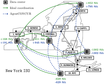
Figure 2: 11-zone NYISO system with 5 data centers. The arrows show active virtual links under different coordination solutions for the 20% NetDC penetration level and 100% maximum latency loss. The change of NetDC electricity demand is given as the average across the test dataset.

The operational data spans the period from January 1, 2018, to June 30, 2019, and includes 546 peak-hour records. Each record contains the following contextual features, which are readily available on the NYISO website [18]:

• Zonal real-time electricity demand $(d)$;

• Zonal electricity prices $(\lambda)$;

• Total renewable generation, then disaggregated by zones using data on existing renewable installations $(r)$;

• Power flows between aggregation zones $(f)$.

Each record includes 45 contextual features, so that the coordination policy based on these features takes the form:

$$\phi\triangleq\beta_{0}+\beta_{1}^{d}\begin{bmatrix}d_{1}\\ \vdots\\ d_{11}\end{bmatrix}+\beta_{1}^{\lambda}\begin{bmatrix}\lambda_{1}\\ \vdots\\ \lambda_{11}\end{bmatrix}+\beta_{1}^{r}\begin{bmatrix}r_{1}\\ \vdots\\ r_{11}\end{bmatrix}+\beta_{1}^{f}\begin{bmatrix}f_{1}\\ \vdots\\ f_{12}\end{bmatrix}$$

To optimize and test the policy, we randomly select $q=250$ records for training and reserve the remaining 296 records for testing, unless stated otherwise. The performance of the trained coordination policies is discussed using the unseen, test set. The remaining settings include default regularization parameters $\varrho=10^{-5}$ and $\varepsilon=10$. All data, codes and default settings needed to replicate the results are available at

https://github.com/wdvorkin/AgentCONCUR

IV-B Efficiency Gains of Power and NetDC Coordination

The NYISO dispatch costs are compared in four cases:

• No coordination: NetDC electricity demand obeys the latency-optimal solution from problem (3);

• Ideal coordination: NetDC demand obeys the solution of the ideal coordination by means of bilevel problem (BL);

• Base regression: NetDC demand is shifted according to the base regression policy optimized in (15);

• AgentCONCUR: NetDC demand is shifted according to the regression policy optimized in (16).

Our results reveal that the NYISO system benefits from coordinating spatial tasks shifts in amount of $\approx 1.9$ GWh from the densely populated South towards the Central, Northern, and Western parts of the state, as shown in Fig. 2. Noticeably, the ideal coordination consistently uses the same 4 out of 10 virtual links, while the AgentCONCUR coordination policy enjoys more active links. This difference is due to less flexible, affine policy structure, which results in more used links to ensure feasibility across the entire training dataset simultaneously, as opposed to per-scenario feasibility satisfaction provided by the ideal coordination.

Figure 3 illustrates the discrepancies in dispatch costs in all four cases. As the penetration of NetDC increases, the non-coordinated solution demonstrates rapid, quadratic growth of dispatch costs in the NYISO dominated by conventional generation. On the other hand, the ideal coordination demonstrates a rather linear growth (e.g., see the bottom plot) of dispatch costs thanks to the cost-aware allocation of computing tasks. However, the extent of cost reduction significantly depends on the maximum allowable latency loss $\alpha,$ specified by the NetDC operator. For a small loss of 25%, users are likely to observe no difference in the quality of service. However, this enables savings of up to 24.5% of dispatch costs in the ideal coordination case, depending on the penetration level. The cost-saving potential increases to 49.0% and 56.7% in the case of double and tripled latency loss, respectively, when users experience more noticeable delays during peak-hour operation.

This cost-saving potential is exploited by both regression coordination policies. However, the base regression policy, which ignores power system and NetDC operational constraints, often results in substantively higher dispatch costs, which tend to stay closer to the non-coordinated solution than to the ideal one. On the other hand, the AgentCONCUR policy, which is aware of constraints of both systems, efficiently approximates the ideal solution, i.e., staying relatively close to the ideal solution in many cases depicted in Fig. 3. However, it tends to show a larger approximation gap as the allowable latency loss and NetDC penetration increase.

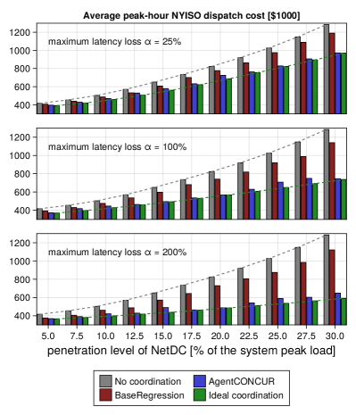
Figure 3: Average NYISO dispatch cost across the testing dataset under different coordination models for the varying NetDC penetration level and maximum allowable latency loss. The area between the dashed lines defines the cost-saving potential for regression-based coordination.

TABLE I: Selected regression features (black dots) for AgentCONCUR for different regularization parameter $\varepsilon$

$\varepsilon$	# of features	zonal electricity demand											power flow												zonal electricity price											zonal renewable power output
		$d_{1}$	$d_{2}$	$d_{3}$	$d_{4}$	$d_{5}$	$d_{6}$	$d_{7}$	$d_{8}$	$d_{9}$	$d_{10}$	$d_{11}$	$f_{1}$	$f_{2}$	$f_{3}$	$f_{4}$	$f_{5}$	$f_{6}$	$\lambda_{7}$	$f_{8}$	$f_{9}$	$f_{10}$	$f_{11}$	$f_{12}$	$\lambda_{1}$	$\lambda_{2}$	$\lambda_{3}$	$\lambda_{4}$	$\lambda_{5}$	$\lambda_{6}$	$\lambda_{7}$	$\lambda_{8}$	$\lambda_{9}$	$\lambda_{10}$	$\lambda_{11}$	$r_{1}$	$r_{2}$	$r_{3}$	$r_{4}$	$r_{5}$	$r_{6}$	$r_{7}$	$r_{8}$	$r_{9}$	$r_{10}$	$r_{11}$
1000.0	29	$\circ$	$\bullet$	$\bullet$	$\bullet$	$\circ$	$\bullet$	$\circ$	$\bullet$	$\bullet$	$\circ$	$\circ$	${\color[rgb]{0,0,0}\bullet}$	$\bullet$	$\bullet$	$\bullet$	$\bullet$	$\bullet$	$\bullet$	$\bullet$	$\bullet$	$\bullet$	$\bullet$	$\circ$	$\bullet$	$\bullet$	$\bullet$	$\bullet$	$\bullet$	$\bullet$	$\bullet$	$\circ$	$\bullet$	$\bullet$	$\circ$	$\circ$	$\bullet$	$\bullet$	$\circ$	$\circ$	$\circ$	$\circ$	$\circ$	$\circ$	$\circ$	$\bullet$
100.0	28	$\bullet$	$\bullet$	$\bullet$	$\bullet$	$\bullet$	$\bullet$	$\circ$	$\bullet$	$\bullet$	$\bullet$	$\circ$	${\color[rgb]{0,0,0}\bullet}$	$\bullet$	$\bullet$	$\bullet$	$\bullet$	$\bullet$	$\bullet$	$\bullet$	$\circ$	$\bullet$	$\circ$	$\circ$	$\circ$	$\bullet$	$\bullet$	$\bullet$	$\bullet$	$\circ$	$\circ$	$\bullet$	$\bullet$	$\bullet$	$\bullet$	$\circ$	$\bullet$	$\circ$	$\circ$	$\circ$	$\circ$	$\circ$	$\circ$	$\circ$	$\circ$	$\bullet$
10.0	24	$\bullet$	$\bullet$	$\bullet$	$\bullet$	$\circ$	$\bullet$	$\bullet$	$\bullet$	$\bullet$	$\bullet$	$\bullet$	${\color[rgb]{0,0,0}\bullet}$	$\bullet$	$\bullet$	$\bullet$	$\circ$	$\bullet$	$\bullet$	$\bullet$	$\bullet$	$\bullet$	$\circ$	$\circ$	$\circ$	$\circ$	$\circ$	$\circ$	$\circ$	$\circ$	$\circ$	$\bullet$	$\bullet$	$\bullet$	$\circ$	$\circ$	$\bullet$	$\circ$	$\circ$	$\circ$	$\circ$	$\circ$	$\circ$	$\circ$	$\circ$	$\bullet$
5.0	20	$\bullet$	$\bullet$	$\circ$	$\bullet$	$\bullet$	$\bullet$	$\bullet$	$\bullet$	$\bullet$	$\bullet$	$\bullet$	${\color[rgb]{0,0,0}\bullet}$	$\bullet$	$\bullet$	$\circ$	$\bullet$	$\circ$	$\bullet$	$\bullet$	$\bullet$	$\circ$	$\circ$	$\circ$	$\circ$	$\circ$	$\circ$	$\circ$	$\circ$	$\circ$	$\circ$	$\circ$	$\bullet$	$\bullet$	$\circ$	$\circ$	$\bullet$	$\circ$	$\circ$	$\circ$	$\circ$	$\circ$	$\circ$	$\circ$	$\circ$	$\circ$
2.5	13	$\bullet$	$\circ$	$\bullet$	$\circ$	$\circ$	$\bullet$	$\bullet$	$\bullet$	$\bullet$	$\bullet$	$\circ$	$\bullet$	$\bullet$	$\circ$	$\circ$	$\circ$	$\bullet$	$\circ$	$\circ$	$\bullet$	$\circ$	$\circ$	$\circ$	$\circ$	$\circ$	$\circ$	$\circ$	$\circ$	$\circ$	$\circ$	$\circ$	$\bullet$	$\bullet$	$\circ$	$\circ$	$\circ$	$\circ$	$\circ$	$\circ$	$\circ$	$\circ$	$\circ$	$\circ$	$\circ$	$\circ$
1.0	6	$\bullet$	$\circ$	$\bullet$	$\circ$	$\circ$	$\circ$	$\circ$	$\circ$	$\circ$	$\bullet$	$\circ$	${\color[rgb]{0,0,0}\bullet}$	$\bullet$	$\circ$	$\circ$	$\circ$	$\circ$	$\circ$	$\circ$	$\circ$	$\bullet$	$\circ$	$\circ$	$\circ$	$\circ$	$\circ$	$\circ$	$\circ$	$\circ$	$\circ$	$\circ$	$\circ$	$\circ$	$\circ$	$\circ$	$\circ$	$\circ$	$\circ$	$\circ$	$\circ$	$\circ$	$\circ$	$\circ$	$\circ$	$\circ$
0.5	3	$\bullet$	$\circ$	$\circ$	$\circ$	$\circ$	$\circ$	$\circ$	$\circ$	$\circ$	$\bullet$	$\circ$	${\color[rgb]{0,0,0}\circ}$	$\circ$	$\bullet$	$\circ$	$\circ$	$\circ$	$\circ$	$\circ$	$\circ$	$\circ$	$\circ$	$\circ$	$\circ$	$\circ$	$\circ$	$\circ$	$\circ$	$\circ$	$\circ$	$\circ$	$\circ$	$\circ$	$\circ$	$\circ$	$\circ$	$\circ$	$\circ$	$\circ$	$\circ$	$\circ$	$\circ$	$\circ$	$\circ$	$\circ$
0.1	1	$\circ$	$\circ$	$\circ$	$\circ$	$\circ$	$\circ$	$\circ$	$\circ$	$\circ$	$\bullet$	$\circ$	${\color[rgb]{0,0,0}\circ}$	$\circ$	$\circ$	$\circ$	$\circ$	$\circ$	$\circ$	$\circ$	$\circ$	$\circ$	$\circ$	$\circ$	$\circ$	$\circ$	$\circ$	$\circ$	$\circ$	$\circ$	$\circ$	$\circ$	$\circ$	$\circ$	$\circ$	$\circ$	$\circ$	$\circ$	$\circ$	$\circ$	$\circ$	$\circ$	$\circ$	$\circ$	$\circ$	$\circ$

IV-C Feasibility of Regression-Based Coordination

The approximation gaps reported in Fig. 3 are due to infeasible task shifts, i.e., the shifts that violate power system constraints, NetDC constraints, or both. Whenever the task shift is infeasible in real-time, the two operators resort to a more expensive yet feasible non-coordinated solution. However, the feasibility of regression-based coordination improves with a larger size of the training dataset, as illustrated in Fig. 4. The AgentCONCUR policy dominates the base one and achieves zero violations of power system constraints (e.g., no load shedding) with sample size $q\geqslant 150$. Moreover, for $q\geqslant 150$, it keeps infeasibility of NetDC operations below 7%. The dominance of AgentCONCUR is consistent, which is important when the set of representative records is limited. We also observed similar results across other NetDC penetration and latency parameters.

Increasing the size of the training dataset also increases the computational burden of problem (16), as shown in Fig. 5. For a reasonable choice of $q=150$, the CPU times are $\approx 8$ hours. However, this time is required for training at the planning stage, i.e., well before the real-time operations.

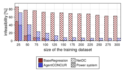
Figure 4: Infeasibility of regression-based coordination as the function of the training dataset size. Results are for 20% NetDC penetration and 25% maximum latency loss, averaged across 100 random draws of training scenarios.

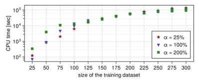
Figure 5: Average CPU times to solve the mixed-integer reformulation of the bilevel program (16). NetDC penetration level is 20%.

IV-D Coordination Feature Selection

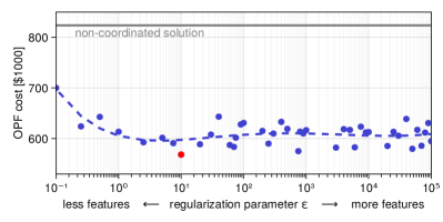
Figure 6: OPF costs for varying regularization parameter $\varepsilon$. The blue dots depict the average costs obtained on the test dataset, and the dash line is the trend. The red dot marks the optimal selection that minimizes the cost on average.

While 45 contextual features are used in training, we demonstrate that the power–NetDC coordination can also be achieved with fewer features, i.e., with less data requirements.

We perform feature selection using regularization parameter $\varepsilon$ in problem (16). The smaller the $\varepsilon$, the fewer features are used by the policy. Table I reports the selected features for various assignments of $\varepsilon$. Observe, as the feature space shrinks ($\downarrow\varepsilon$), the policy gives less priority to renewable power data, which is reasonable as the NYISO has a very small installed renewable capacity at present (e.g., only 1.7 GW). As the space further shrinks, less priority is given to electricity prices, which become less informative in uncongested cases. The power flows and electricity demands, on the other hand, consistently present among selected features for AgentCONCUR.

Figure 6 further reveals the trade-off between the dispatch cost and amount of selected features. Approximately, the same level of costs (see the dashed trend line) can be achieved in the range $\varepsilon\in[1,10^{5}]$, selecting from 6 to $30+$ features. Moreover, parameter $\varepsilon$ can be optimized to achieve the optimal dispatch cost under regression-based coordination. Here, the optimal $\varepsilon^{\star}=10$ selects 24 features for coordination.

Notably, for $\varepsilon=0.1$, the coordination of task shifts within the entire NetDC is performed with a single feature, i.e., electricity demand of the largest demand center – New York City. Although this is not the cost-optimal choice, this is the least data-intensive coordination, which still performs better than the non-coordinated solution, as also shown in Fig. 6.

V Conclusions

To streamline the economic coordination of power grids and data centers, this work proposed to transition from data-intensive optimization-based coordination to a light weighted regression-based coordination. Recognizing the risks of trusting a regression model with coordinating two critical infrastructure systems, we devised a new training algorithm which inherits the structure of the optimization-based coordination and enables feasible and cost-consistent computing task shifts in real-time. The case study on NYISO system with various NetDC penetration levels revealed 24.5–56.7% cost-saving potential, most of which has shown to be delivered by regression policies at different data-intensity preferences.

There are some notable limitations that motivate several directions for future work. First, while the optimization-based coordination remunerates data center flexibility via duality theory [11], as such, the duality-based solution is unavailable under regression policies. It is thus relevant to study the integration of regression policies into real-time electricity markets. Moreover, while the current focus has been on spatial flexibility for peak-hour coordination, it is also relevant to explore regression policies for harnessing both spatial and temporal flexibility, as proposed before for optimization-based coordination [9]. This, in turn, may result in the increased computational burden and require decomposition. Lastly, although the proposed mechanism does not require any private data exchange at the time of coordination, it still needs sensitive data from the power system and NetDC for training at the planning stage. One potential solution to remove this practical bottleneck is the use of data obfuscation algorithms [22], yet it will require additional modifications to the training procedure to eliminate the effect of noise.

References

- [1] A. Papavasiliou and I. Mezghani, “Coordination schemes for the integration of transmission and distribution system operations,” in Power Systems Computation Conference, 2018, pp. 1–7.
- [2] A. Ratha et al., “Affine policies for flexibility provision by natural gas networks to power systems,” Electr. Power Syst. Res., vol. 189, 2020.
- [3] L. Mitridati and J. A. Taylor, “Power systems flexibility from district heating networks,” in Power Systems Computation Conference, 2018.
- [4] A. Wierman et al., “Opportunities and challenges for data center demand response,” in Internat. Green Computing Conference, 2014, pp. 1–10.
- [5] McKisey and Company. (2023) Investing in the rising data center economy. [Online]. Available: http://tinyurl.com/mppbbh4h
- [6] D. Patterson et al., “Carbon emissions and large neural network training,” arXiv preprint arXiv:2104.10350, 2021.
- [7] A. James and D. Schien, “A low carbon kubernetes scheduler.” in 6th International Conference on ICT for Sustainability, 2019.
- [8] A. Radovanović et al., “Carbon-aware computing for datacenters,” EEE Trans. Power Syst., vol. 38, no. 2, pp. 1270–1280, 2022.
- [9] W. Zhang et al., “Flexibility from networks of data centers: A market clearing formulation with virtual links,” Electr. Power Syst. Res., vol. 189, p. 106723, 2020.
- [10] K. Kim et al., “Data centers as dispatchable loads to harness stranded power,” IEEE Trans. Sustain. Energy, vol. 8, no. 1, pp. 208–218, 2016.
- [11] W. Zhang and V. M. Zavala, “Remunerating space–time, load-shifting flexibility from data centers in electricity markets,” Appl. Energy, vol. 326, p. 119930, 2022.
- [12] M. Muñoz, S. Pineda, and J. Morales, “A bilevel framework for decision-making under uncertainty with contextual information,” Omega, vol. 108, p. 102575, 2022.
- [13] V. Dvorkin and F. Fioretto, “Price-aware deep learning for electricity markets,” arXiv preprint arXiv:2308.01436, 2023.
- [14] S. Chatzivasileiadis, “Lecture notes on optimal power flow (OPF),” arXiv preprint arXiv:1811.00943, 2018.
- [15] A. Radovanovic et al., “Power modeling for effective datacenter planning and compute management,” IEEE Trans. Smart Grid, vol. 13, no. 2, pp. 1611–1621, 2021.
- [16] I. Narayanan, A. Kansal, and A. Sivasubramaniam, “Right-sizing geo-distributed data centers for availability and latency,” in 37th International Conference on Distributed Computing Systems, 2017, pp. 230–240.
- [17] D. Pozo, E. Sauma, and J. Contreras, “Basic theoretical foundations and insights on bilevel models and their applications to power systems,” Ann. Oper. Res., vol. 254, pp. 303–334, 2017.
- [18] NYISO. (2023) Energy market & operational data. [Online]. Available: https://www.nyiso.com/energy-market-operational-data
- [19] R. Tibshirani, “Regression shrinkage and selection via the lasso,” J. R. Stat. Soc., B: Stat., vol. 58, no. 1, pp. 267–288, 1996.
- [20] A. Nemirovski and A. Shapiro, “Convex approximations of chance constrained programs,” SIAM Journal on Optimization, vol. 17, no. 4, pp. 969–996, 2007.
- [21] H. A. U. Khan, J. Kim, and Y. Dvorkin, “Risk-informed participation in T&D markets,” Electr. Power Syst. Res., vol. 202, p. 107624, 2022.
- [22] V. Dvorkin and A. Botterud, “Differentially private algorithms for synthetic power system datasets,” IEEE Control Systems Letters, 2023.
- [23] S. Siddiqui and S. A. Gabriel, “An SOS1-based approach for solving MPECs with a natural gas market application,” Netw. Spat. Econ., vol. 13, pp. 205–227, 2013.