A note on the Hamiltonian structure of transgression forms

Abstract

By incorporating two gauge connections, transgression forms provide a generalization of Chern-Simons actions that are genuinely gauge-invariant on bounded manifolds. In this work, we show that, when defined on a manifold with a boundary, the Hamiltonian formulation of a transgression field theory can be consistently carried out without the need to implement regularizing boundary terms at the level of first-class constraints. By considering boundary variations of the relevant functionals in the Poisson brackets, the surface integral in the very definition of a transgression action can be translated into boundary contributions in the generators of gauge transformations and diffeomorphisms. This prescription systematically leads to the corresponding surface charges of the theory, reducing to the general expression for conserved charges in (higher-dimensional) Chern-Simons theories when one of the gauge connections in the transgression form is set to zero.

1 Introduction

Chern-Simons (CS) forms have been extensively used in the construction of action principles in different areas of physics (see [1, 2, 3, 4, 5, 6] and references therein). In the context of gravity, CS forms can be used to define (super-)gravity theories in odd dimensions as genuine gauge theories [7, 8, 9, 10] (for a detailed analysis, see also [11, 12]). However, when gauge fields are defined on a manifold with a boundary, CS actions become quasi-gauge-invariant. In other words, under gauge transformations, they change in an exact form. In order to restore gauge invariance, boundary terms can be added to the action (see, for instance, [13, 14]). Furthermore, boundary terms together with boundary conditions on the fields are generally necessary for the action to have a well-defined variation and be a true extremum when the field equations hold [15]. In the case of three-dimensional CS gravity with a negative cosmological constant, this procedure generally leads to a (reduced) Wess-Zumino-Witten (WZW) model defined at the two-dimensional boundary [16]. These results have been generalized to the five-dimensional case [17], where a WZW₄ model is shown to arise at the boundary when suitable boundary conditions are adopted. The study of gauge theories defined on bounded manifolds has attracted considerable attention in the last decades due to the advent of the holographic principle [18, 19] and the AdS/CFT correspondence [20]. In this context, bulk/boundary dualities in CS theories have led to remarkable results in the direction of a holographic description of three-dimensional gravity (see, for example, [21, 22, 23, 24]). Moreover, in recent years, different aspects of dual field theories associated to higher-dimensional AdS CS gravities have been explored [25, 26, 27].

When applying Dirac’s Hamiltonian formalism for constrained systems [28, 29] to CS theories in the presence of a boundary, conserved charges appear as surface integrals that, provided a set of boundary conditions, regularize the first-class constraints of the system and allow one to find a surface charge algebra once the gauge is appropriately fixed and the Dirac brackets are implemented. This is nothing but a particular example of the prescription due to Regge and Teiteilboim [15] applied to gauge theories. Moreover, in $2+1$ dimensions, the Hamiltonian formalism for CS theories is generic, i.e. the rank of the symplectic form that defines the phase space of the theory is constant, and the corresponding Dirac brackets can be globally defined [30, 31]. After imposing suitable boundary conditions on the CS gauge connection, one can find the surface charge algebra of the theory from the Dirac brackets of the regularized first-class constraints. On the other hand, in higher dimensions, the situation changes completely, and the Hamiltonian dynamics of the theory is highly non-trivial. This is because, for $D\geq 5$, the CS symplectic form has a non-constant rank throughout the phase space, dividing this into sectors possessing different numbers of local degrees of freedom. The Hamiltonian formulation, in this case, can be used to find the conserved charges once a generic and regular sector of the theory has been chosen, and the constraints of the theory can be adequately split into first- and second-class [32, 33].

Transgression forms first appeared in physics in the topological interpretation of anomalies in quantum field theory and gravity [34, 35]. In the context of gravitational gauge theories, transgression field theory (TrFT) can be used to define (super-)gravity action principles in odd dimensions that are genuinely gauge invariant [36, 37, 38, 39], whereas, in the even-dimensional case, TrFTs allow one to define gauged-WZW models and topological gravity theories [40, 41, 42, 43, 44, 45]. Being genuinely gauge-invariant, it is possible to define conserved charges in TrFTs through Noether’s theorem straightforwardly. Transgression forms can be constructed by subtracting two CS forms plus a boundary term, rendering the theory gauge invariant. Therefore, it is reasonable to expect that in the case of a TrFT, the boundary term in its very definition is sufficient to obtain the corresponding conserved charges as surface integrals in the symmetry generators through Dirac’s algorithm. In this article, we will show that, provided the boundary variations of the relevant functionals are consistently treated, this is indeed the case.

As stated before, the usual criteria when applying the Regge-Teitelboim method to gauge theories is to include regularizing boundary terms in the first-class constraints [46, 47, 21] so that their variations do not drop boundary terms and their Poisson brackets lead to regularized functionals as well [48]. However, to apply the Hamiltonian formulation for constrained systems to an action based on a transgression form and not to lose the information contained in the transgression boundary term during the process, one should necessarily allow boundary contributions in the variations of the constraints of the theory. As shown by Soloviev and Bering [49, 50] (see also [51]), treating functionals with boundary variations requires carefully extending the definition of the usual Poisson bracket to the boundary of the space-time manifold. This is mainly due to the fact that when boundary variations are allowed, the Poisson bracket does not fulfil the Jacobi identity [53]. Based on these results, we will analyze TrFT applying Dirac’s formalism for constrained systems and including the boundary variations of the phase space functionals throughout. The inclusion of boundary variations in the Poisson brackets effectively leads to a Hamiltonian formulation based on the modified Poisson bracket proposed by Soloviev and Bering [49, 50]. We will show that this procedure allows us to recover the conserved charges of TrFT from the resulting boundary terms in the first-class constraints of the theory.

This paper is organized as follows. Section 2 will briefly review the definition of transgression forms and their relation to CS theory. In Section 3, we give a short summary of the Hamiltonian formulation of CS theories. We introduce a generalized Poisson bracket and use it to apply Dirac’s algorithm for constrained systems to TrFT. In Section 4, we apply this prescription to transgression forms in three and five dimensions and show that the boundary terms obtained in the first-class constraints allow us to recover the conserved charges of the theory. In Section 5, we conclude with an analysis of the results and discuss possible future directions.

2 Transgression Forms

We start by briefly surveying the properties of transgression forms and TrFT. This summary makes no pretence of being complete or up-to-date. More detailed analysis can be found in the references (see, for instance, [54, 55]).

Given a principal bundle with fibre $G$ over a $(2n+2)$-dimensional base manifold and a connection one-form $A$ defined on it, one can always construct an invariant polynomial $P(F)$ out of the $(n+1)$-th wedge power of the curvature two-form $F=dA+A^{2}$ associated with $A$, which is usually expressed as

$$P(F)=\langle F\ldots F\rangle\;,$$ (2.1)

where $\langle\dots\rangle$ stands for an invariant symmetric multilinear form on the Lie algebra $\mathfrak{g}$ associated with the Lie group $G$. By definition, the polynomial (2.1) is a $(2n+2)$-form invariant under gauge transformations $F\rightarrow g^{-1}Fg$ where $g\in G$. The Chern-Weil theorem [55] ensures that $P(F)$ is closed [$dP(F)=0$] and that, if $F$ and $\bar{F}$ are the curvatures corresponding to two different connections $A$ and $\bar{A}$ on the same principal bundle, $P(F)-P(\bar{F})$ is exact, i.e.

$$P(F)-P(\bar{F})=d\mathcal{T}_{2n+1}\ .$$ (2.2)

This defines the transgression form

$$\mathcal{T}_{2n+1}\left[A,\bar{A}\right]=(n+1)\int_{0}^{1}dt\ \left\langle\left({A-}\bar{A}\right)F_{t}^{n}\right\rangle\;,$$ (2.3)

where $t\in[0,1]$, $A_{t}=tA+(1-t)\bar{A}$ is a connection that interpolates between $A$ and $\bar{A}$, and $F_{t}=dA_{t}+A_{t}^{2}$ is the corresponding interpolating curvature [34, 35] (for details on the mathematical definition of the transgression see [54, 55]). From equation 2.3, it is straightforward to show that the transgression form is gauge-invariant. It is important to note that setting $\bar{A}=0$ leads to the CS $(2n+1)$-form

$$CS_{2n+1}\left[A\right]=\mathcal{T}_{2n+1}\left[A,0\right]=(n+1)\int_{0}^{1}dt\ \left\langle A\left(tdA+t^{2}A^{2}\right)^{n}\right\rangle\;.$$ (2.4)

Furthermore, the transgression form (2.3) can be written as the difference of two CS forms plus an exact term

$$\mathcal{T}_{2n+1}\left[A,\bar{A}\right]=CS_{2n+1}\left[A\right]-CS_{2n+1}\left[\bar{A}\right]-d\mathcal{B}_{2n}\left[A,\bar{A}\right]\;,$$ (2.5)

where $\mathcal{B}_{2n}$ is given by

$$\mathcal{B}_{2n}=-n(n+1)\int_{0}^{1}ds\int_{0}^{1}dts\left\langle A_{t}(A-\bar{A})F_{st}^{n-1}\right\rangle,\quad F_{st}=sF_{t}+s(s-1)A_{t}^{2}\;.$$ (2.6)

At this point it is important to remember that the CS form (2.4) is not strictly gauge-invariant, but quasi-invariant. Indeed, its variation under gauge transformations of the gauge connections $A$ and $\bar{A}$ drops an exact form. It is precisely the boundary term in equation 2.5 that makes the transgression a truly gauge-invariant form. Due to this property, transgression forms have been used to define gauge-invariant actions for field theories and gravity in diverse dimensions [36, 37, 38].

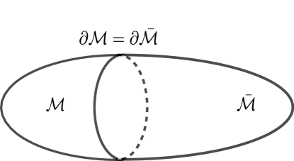
Figure 1: Cobordant manifolds. Two manifolds $\mathcal{M}$ and $\bar{\mathcal{M}}$ having a common boundary $\partial\mathcal{M}=\partial\bar{\mathcal{M}}$.

A TrFT is a field theory whose action is constructed out of a transgression form. Different variants of TrFT can be defined depending on the way the gauge connections $A$ and $\bar{A}$ are treated. For instance, one could consider $A$ and $\bar{A}$ as respectively defined on two different $(2n+1)$-dimensional manifolds, $\mathcal{M}$ and $\bar{\mathcal{M}}$, that are cobordant, i.e. $\partial\mathcal{M}=\partial\bar{\mathcal{M}}$ (see Figure 1). The principal bundle with fiber $G$ can then be defined on the manifold $\mathcal{M}+\bar{\mathcal{M}}$ and the definition (2.5) can be used to define the following action principle for a TrFT [38]

$$I\left[A,\bar{A}\right]=\kappa\int_{\mathcal{M}}CS_{2n+1}\left[A\right]-\kappa\int_{\mathcal{\bar{M}}}CS_{2n+1}\left[\bar{A}\right]-\kappa\int_{\partial\mathcal{M}}\mathcal{B}_{2n}\left[A,\bar{A}\right]\ ,$$ (2.7)

where $\kappa$ is a constant. In general, one can allow the connections $A$ and $\bar{A}$ to transform with different group elements, provided they match at the boundary, i.e. the action (2.7) is invariant under transformations of the form

$$A\longrightarrow gAg^{-1}-dgg^{-1}\ ,\quad\bar{A}\longrightarrow\bar{g}A\bar{g}^{-1}-d\bar{g}\bar{g}^{-1}\ ,\quad g\Big{|}_{\partial\Sigma}=\bar{g}\Big{|}_{\partial\Sigma}\ .$$ (2.8)

In the case of infinitesimal gauge transformations, where $g=\mathbb{1}+\eta$, $\bar{g}=\mathbb{1}+\bar{\eta}$, and $\eta,\ \bar{\eta}\,\in\mathfrak{g}$, this means

$$\delta A=-D\eta\ ,\quad\delta\bar{A}=-\bar{D}\bar{\eta}\ ,\quad\eta\Big{|}_{\partial\Sigma}=\bar{\eta}\Big{|}_{\partial\Sigma}\;.$$ (2.9)

The action (2.7) has been used to generalize CS gravitational theories, providing the conserved charges of the theory and the correct expression for black hole thermodynamics when suitable boundary conditions are adopted [36, 38, 56].

Another type of TrFT can be constructed by considering both connections, $A$ and $\bar{A}$, as defined on the same base manifold, i.e. $\mathcal{M}=\bar{\mathcal{M}}$. In particular, one can consider $A$ and $\bar{A}$ as belonging to the same gauge orbit, $\bar{A}=A^{h}=hAh^{-1}-dhh^{-1}$, where $h\in G$ (see Figure 2). In this case, a TrFT reduces to a gauged WZW model living at the boundary [40, 42, 44, 45].

In this work, we will consider the connections $A$ and $\bar{A}$ as independent, but defined on the same manifold $\mathcal{M}$. However, the results can be easily generalized to the case of cobordant manifolds discussed above. Considering $\mathcal{M}=\bar{\mathcal{M}}$ in equation 2.7 allows one to write the TrFT action as simply the integral of the transgression form (2.5) over $\mathcal{M}$,

$$I\left[A,\bar{A}\right]=\kappa\int_{\mathcal{M}}\mathcal{T}_{2n+1}\left[A,\bar{A}\right]\;.$$ (2.10)

Figure 2: Gauged WZW case. A single manifold $\mathcal{M}$ where two connections $A$ and $A^{h}$ are defined, belonging to their respective spaces $G_{p}$ and $G^{\prime}_{p}$ at $p\in\mathcal{M}$. $A$ and $A^{h}$ are connected by a gauge transformation defined by an element $h\in G$, where $G$ is the strucutre group.

3 Hamiltonian structure of transgression field theory

In this section, we apply Dirac’s formalism for constrained systems to the TrFT defined by the action (2.10). Since the boundary term in the definition of the transgression form guarantees the gauge invariance of the theory, we will consider all the contributions coming from this term throughout the Hamiltonian formalism and will not add any regularizing boundary term to the constraints by hand. This procedure can be implemented by defining a generalized Poisson bracket that takes into account the boundary variations of the phase space functionals. This bracket was introduced by Soloviev and Bering in references [49] and [50]. By means of this generalized bracket, the boundary terms present in the transgression action will be shown to lead to surface integrals for the first-class constraints of the theory. The generators of the symmetry transformations constructed in terms of these first-class constraints form a Poisson algebra isomorphic to the corresponding symmetry algebras of the theory under the modified Poisson bracket. Furthermore, its surface integrals provide a general formula for the conserved charges of the theory. The important point in this derivation is that it does not need to adopt any “a priori” boundary conditions on the fields or regularizing boundary terms.

3.1 Review of Chern-Simons theories

Let us start reviewing the Hamiltonian formulation of (higher-dimensional) CS theories. We will consider a $(2n+1)$-dimensional space-time without boundary and with topology $\mathcal{M}=\mathbb{R}\times\Sigma$, where $\mathbb{R}$ corresponds to the real (temporal) line and $\Sigma$ is a $2n$-dimensional spatial hypersurface. We denote the infinitesimal generators of $G$ as $T_{a}$, which satisfy

$$[\![T_{a},T_{b}]\!]=f^{c}_{ab}T_{c}\ ,\qquad\left\langle T_{a_{1}}\cdots T_{a_{n+1}}\right\rangle=g_{a_{1}\cdots a_{n+1}}\;,\quad a=1,\dots,{\rm dim}\,\mathfrak{g}\;,$$ (3.1)

with $f^{c}_{ab}$ the structure constants of the Lie algebra $\mathfrak{g}$ ang $g_{a_{1}\cdots a_{n+1}}$ an invariant symmetric $(n+1)$-rank tensor. In this case, a connection one-form taking values on $\mathfrak{g}$ can be split as

$$A =A_{\mu}^{a}T_{a}dx^{\mu}=A_{0}^{a}T_{a}dx^{0}+A_{i}^{a}T_{a}dx^{i}\ .$$ (3.2)

The CS action (2.4) can be written in Hamiltonian form [57, 33],

$$I_{H}\left[A\right]=\int dx^{0}\int_{\Sigma}d^{2n}x\;\left[\mathcal{L}_{a}^{i}\left(A\right)\dot{A}_{i}^{a}+A_{0}^{a}K_{a}\left(A\right)\right]\ ,$$ (3.3)

where the Gauss law constraint $K_{a}$ is given by

$$K_{a}\left(A\right)=\frac{\kappa}{2^{n}}\left(n+1\right)\epsilon^{i_{1}i_{2}\cdots i_{2n-1}i_{2n}}g_{ab_{1}\cdots b_{n}}F_{i_{1}i_{2}}^{b_{1}}\cdots F_{i_{2n-1}i_{2n}}^{b_{n}}\ ,$$ (3.4)

and $\mathcal{L}_{a}^{i}$ is a function of $A_{i}$ that determines the phase space symplectic form

$$\Omega^{ij}_{ab}=\dfrac{\delta\mathcal{L}_{b}^{j}}{\delta A_{i}^{a}}-\dfrac{\delta\mathcal{L}_{a}^{i}}{\delta A_{j}^{b}}=-\dfrac{\kappa\,n\left(n+1\right)}{2^{n-1}}\epsilon^{ijk_{1}k_{2}\cdots k_{2n-3}k_{2n-2}}g_{abc_{1}\cdots c_{n-1}}F_{k_{1}k_{2}}^{c_{1}}\cdots F_{k_{2n-3}k_{2n-2}}^{c_{n-1}}\ .$$ (3.5)

The phase space of the theory is defined by the spatial components of the connection $A^{a}_{i}$ and its canonically conjugated momenta $\pi_{a}^{i}$, with canonical Poisson brackets

$$\left\{A_{\mu}^{a}(x),\pi_{b}^{\nu}\left(y\right)\right\}=\delta_{b}^{a}\delta_{\mu}^{\nu}\delta^{\left(2n\right)}\left(x-y\right)\,.$$ (3.6)

When applying Dirac’s Hamiltonian formalism [28, 29], the definition of canonical momenta leads to the following primary constraints

$$\phi^{0}_{a} = \pi^{0}_{a}\approx 0\ ,$$ (3.7)

$$\phi^{i}_{a} = \pi^{i}_{a}-\mathcal{L}_{a}^{i}(A)\approx 0\ ,$$ (3.8)

whereas the corresponding primary Hamiltonian reads

$$H=H_{0}+\int_{\Sigma}d^{2n}x\;\left[\lambda^{a}\phi^{0}_{a}+\Lambda^{a}_{i}\phi^{i}_{a}\right]\ ,$$ (3.9)

where

$$H_{0}=-\mathcal{\kappa}\int_{\Sigma}d^{2n}x\;\,A_{0}^{a}K_{a}\left(A\right)\ ,$$

is the canonical Hamiltonian and $\lambda^{a}$, $\Lambda^{a}_{i}$ are Lagrange multipliers. Time preservation of $\phi^{0}_{a}$ generates the secondary constraint $K_{a}(A)\approx 0$, while time preservation of $\phi^{i}_{a}$ leads to no new constraints, but fixes the Lagrange multipliers $\Lambda_{i}\approx D_{i}A_{0}$ in the primary Hamiltonian. The first-class constraints of the theory can be found by redefining $K_{a}$ in the form

$$G_{a}=K_{a}+D_{i}\phi_{a}^{i}\;,$$ (3.10)

which generates the correct infinitesimal gauge transformations

$$\delta A^{a}_{i}(x)=\left\{A_{i}^{a}(x),\int_{\Sigma}d^{2n}y\;\,\eta^{b}(y)G_{b}(y)\right\}=-D_{i}\eta^{a}(x)\,.$$ (3.11)

Moreover, together with the second-class constraints $\phi_{a}^{i}$, the constraints satisfy the Poisson algebra

$$\{G_{a},G_{b}\}=f^{c}_{ab}G_{c}\,,\quad\{G_{a},\phi_{b}^{i}\}=f^{c}_{ab}\phi_{c}^{i}\,,\quad\{\phi_{a}^{i},\phi_{b}^{j}\}=\Omega_{ab}^{ij}\,.$$ (3.12)

The CS actions are also invariant under diffeomorphisms

$$\delta A^{a}_{i}(x)=\left\{A_{i}^{a}(x),\int_{\Sigma}d^{2n}y\;\,\zeta^{i}(y)L_{i}(y)\right\}=-\mathfrak{L}_{\zeta}A^{a}_{i}\ ,$$ (3.13)

where $\mathfrak{L}_{\zeta}$ stands for the Lie derivative along a spatial vector field $\zeta=\zeta^{i}\partial_{i}$. Using the identity

$$\mathfrak{L}_{\zeta}A^{a}_{i}=-F^{a}_{ij}\zeta^{j}+D_{i}\left(\zeta^{j}A^{a}_{j}\right)\ ,$$ (3.14)

one can see that the generator of infinitesimal spatial diffeomorphisms can be constructed as the following combination of the constraints

$$L_{i}=\mathcal{H}_{i}+A^{a}_{i}G_{a}\ ,\qquad\mathcal{H}_{i}=-F^{a}_{ij}\phi_{a}^{j}\ .$$ (3.15)

Note that $\mathcal{H}_{i}$ generates the so-called improved spatial diffeomorphisms [58], namely, $\delta A_{i}=-F_{ij}\zeta^{j}$. Time-like diffeomorphisms, on the other hand, can be shown to be generated by a combination of $G_{a}$ and $\mathcal{H}_{i}$ [57]. From equation 3.15 it is clear that a diffeomorphism with parameter $\zeta^{i}$ can be written as an improved diffeomorphism plus a gauge transformation with a field-dependent parameter $\eta^{a}=\zeta^{i}A^{a}_{i}$.

The dynamical structure of the $(2+1)$-dimensional theory is quite simple in comparison with higher dimensional cases. In fact, for $n=1$, the symplectic form in equation 3.5 can be inverted, implying that the constraints $\phi_{a}^{i}$ are second-class and can be set strongly to zero after implementing Dirac brackets. This leads to a canonical bracket for the reduced-phase space variables $A^{a}_{i}$. Once the constraints $\phi_{a}^{i}$ are eliminated, the gauge generator (3.10) reduces to the Gauss law constraint $G_{a}=K_{a}$, while $\mathcal{H}_{i}$ vanishes, implying that in three space-time dimensions diffeomorphisms are on-shell equivalent to gauge transformations. For $n\geqslant 2$, on the other hand, the symplectic form $\Omega_{ab}^{ij}$ is degenerate [57, 32, 33] (see also [59, 60, 61, 62] for details on degenerate Hamiltonian systems), which means that in higher odd-dimension, the phase space of CS theories is divided in sectors that are dynamically disconnected. Furthermore, the constraints may be irregular [63]. In generic and regular sectors, there are $2n$ null eigenvectors $(v_{i})_{j}=F_{ij}$. This leads the first-class constraints $\mathcal{H}_{i}$ in equation 3.15, which are independent of the gauge generators $G_{a}$. In non-generic sectors, there are even more first-class constraints, which generate so-called accidental symmetries. These will not be considered here.

3.2 Poisson brackets and boundary terms

In order to apply Dirac formalism to a TrFT and keep contributions coming from the boundary term (2.6) throughout, we will not use the standard Regge-Teitelboim prescription [15] based on regularized functionals, as it requires introducing a different boundary term in the action (2.7) depending on the boundary conditions chosen for the gauge fields [46, 47, 21, 48] (see [64] for a detailed analysis). Instead, we will consider a generalized Poisson bracket that includes the boundary variations of the relevant functionals in a consistent way. Brackets of this kind were proposed first by Soloviev [49], and later on by Bering [50] in the study of Hamiltonian systems defined on spaces with boundaries.

Let us consider a functional $F$ of some set of fields $\psi^{A}$ and their derivatives $\partial_{i}\psi^{A}$, defined on a $d$-dimensional spatial section $\Sigma$ with boundary $\partial\Sigma$

$$F\left[\psi\right]=\int_{\Sigma}d^{d}x\,\mathcal{F}\left(\psi^{A}(x),\partial_{i}\psi^{A}(x)\right)+\int_{\partial\Sigma}d^{d-1}x\;\hat{n}_{i}\,f^{i}\left(\psi^{A}(x),\partial_{i}\psi^{A}(x)\right)\ ,$$ (3.16)

where $\hat{n}_{i}$ is a unitary vector normal to $\partial\Sigma$. This means that the variation of $F$ with respect to $\psi^{A}$ drops a boundary term of the form

$$\delta F\left[\psi\right] =\int_{\Sigma}d^{d}x\left[\frac{\partial\mathcal{F}}{\partial\psi^{A}}-\partial_{i}\left(\frac{\partial\mathcal{F}}{\partial\left(\partial_{i}\psi^{A}\right)}\right)\right]\delta\psi^{A}$$ (3.17)

$$+\int_{\partial\Sigma}d^{d-1}x\;\hat{n}_{i}\,\left[\frac{\partial f^{i}}{\partial\psi^{A}}-\partial_{j}\left(\frac{\partial f^{i}}{\partial\left(\partial_{j}\psi^{A}\right)}\right)+\frac{\partial\mathcal{F}}{\partial\left(\partial_{i}\psi^{A}\right)}\right]\delta\psi^{A}\ .$$

Usually, in this case, one would like to add a surface integral to $F$ such that, provided certain boundary conditions on the fields $\psi^{A}$, $\delta F$ does not drop any boundary term. This would ensure the closure of Poisson brackets [48]. Nevertheless, if this procedure is to be applied to the transgression action, one should dump the boundary terms (2.6) and later add regularizing boundary terms to the first-class constraints of the theory. Eliminating this boundary term turns equation 2.7 into the sum of two CS forms, yielding to the usual Hamiltonian formalism for CS theories described in Section 3.1. Here, instead, we would like to exploit the properties of the transgression form by keeping its boundary term untouched and dragging its information through the Dirac formalism. Thus, we will not adopt any boundary conditions for the fields and keep all the boundary terms appearing in the variations of the functionals. When considering variations of the form (3.17), however, the usual Poisson bracket does not fulfill the Jacobi identity. The reason for this is that functional derivatives do not commute in the presence of a boundary [53]. A Poisson bracket that satisfies the Jacobi identity and takes into account these boundary contributions can be constructed by following the works of Soloviev and Bering in references [49, 50]. In order to do that, the bulk and boundary parts of equation 3.17 are to be considered as the bulk and boundary functional derivatives of $F$, denoted by $\hat{\delta}F/\delta\psi^{A}$ and $\check{\delta}F/\delta\psi^{A}$, respectively,

$$\delta F\left[\psi\right]=\int_{\Sigma}d^{d}x\;\frac{\hat{\delta}F}{\delta\psi^{A}}\delta\psi^{A}+\int_{\partial\Sigma}d^{d-1}x\;\frac{\check{\delta}F}{\delta\psi^{A}}\delta\psi^{A}\ ,$$ (3.18)

where

$$\frac{\hat{\delta}F}{\delta\psi^{A}}=\frac{\delta\mathcal{F}}{\delta\psi^{A}},\qquad\frac{\check{\delta}F}{\delta\psi^{A}}=\hat{n}_{i}\left(\frac{\delta f^{i}}{\delta\psi^{A}}+\frac{\partial\mathcal{F}}{\partial\left(\partial_{i}\psi^{A}\right)}\right)\ .$$ (3.19)

Here we have used the notation

$$\frac{\delta X}{\delta\psi^{A}}=\frac{\partial X}{\partial\psi^{A}}-\partial_{j}\left(\frac{\partial X}{\partial\left(\partial_{j}\psi^{A}\right)}\right)\ .$$ (3.20)

Then, given a symplectic structure for the phase space of the theory $\omega_{AB}$, the Poisson bracket of $F$ with some field $\psi^{A}$ can then be extended to the boundary, i.e.

$$\left\{F,\psi^{A}(x)\right\}=\int_{\Sigma}d^{d}y\;\frac{\hat{\delta}F(y)}{\delta\psi^{B}(x)}\omega^{BA}+\int_{\partial\Sigma}d^{d-1}y\;\frac{\check{\delta}F(y)}{\delta\psi^{B}(x)}\omega^{BA}\ ,$$ (3.21)

where $\omega^{AB}$ is the inverse of $\omega_{AB}$, and defines the Poisson bracket

$$\{\psi^{A}(x),\psi^{B}(y)\}=\omega^{AB}\delta^{(d)}(x-y)\ .$$ (3.22)

For a function $\mathcal{F}(x)$ depending of $\psi^{A}$ and its derivatives, one finds

$$\{\mathcal{F}(x),\psi^{A}(y)\}=\int_{\Sigma}d^{d}z\left[\frac{\partial\mathcal{F}(x)}{\partial\psi^{B}(z)}\{\psi^{B}(z),\psi^{A}(y)\}+\frac{\partial\mathcal{F}(x)}{\partial(\partial_{i}^{(z)}\psi^{B}(z))}\{\partial_{i}^{(z)}\psi^{B}(z),\psi^{A}(y)\}\right]$$ (3.23)

$$=\frac{\delta\mathcal{F}(x)}{\delta\psi^{B}(y)}\omega^{BA}+\int_{\Sigma}d^{d}z\,\partial_{i}^{(z)}\left(\frac{\partial\mathcal{F}(x)}{\partial(\partial_{i}^{(z)}\psi^{B}(z))}\,\omega^{BA}\,\delta^{(D)}(z-y)\right)\ .$$

Thus, for two functions $\mathcal{F}$ and $\mathcal{G}$, this leads to

$$\{\mathcal{F}(x),\mathcal{G}(y)\}=\int_{\Sigma}d^{d}z\frac{\delta\mathcal{F}(x)}{\delta\psi^{B}(z)}\{\psi^{B}(z),\mathcal{G}(y)\}+\int_{\Sigma}d^{d}z\;\partial_{i}^{(z)}\left(\frac{\partial\mathcal{F}(x)}{\partial(\partial_{i}^{(z)}\psi^{B}(z))}\{\psi^{B}(z),\mathcal{G}(y)\}\right)$$ (3.24)

$$=\int_{\Sigma}d^{d}z\bigg{[}\frac{\delta\mathcal{F}(x)}{\delta\psi^{A}(z)}\omega^{AB}\frac{\delta\mathcal{G}(y)}{\delta\psi^{B}(z)}+\partial_{i}^{(z)}\left(\frac{\delta\mathcal{F}(x)}{\delta\psi^{A}(z)}\omega^{AB}\frac{\mathcal{G}(y)}{\partial(\partial_{i}^{(z)}\psi^{B}(z))}+\frac{\partial\mathcal{F}(x)}{\partial(\partial_{i}^{(z)}\psi^{A}(z))}\omega^{AB}\frac{\delta\mathcal{G}(y)}{\delta\psi^{B}(z)}\right)\bigg{]}\ .$$

On the other hand, for two functionals of the form (3.16), i.e.

$$F\left[\psi\right] =\int_{\Sigma}d^{d}x\,\mathcal{F}(x)+\int_{\partial\Sigma}d^{d-1}x\;\hat{n}_{i}\,f^{i}(x)\ ,$$ (3.25)

$$G\left[\psi\right] =\int_{\Sigma}d^{d}y\,\mathcal{G}(y)+\int_{\partial\Sigma}d^{d-1}y\;\hat{n}_{i}\,g^{i}(y)\ ,$$

one finds

$$\{F,G\}=\int_{\Sigma}d^{d}x\int_{\Sigma}d^{d}y\{\mathcal{F}(x),\mathcal{G}(y)\}+\int_{\Sigma}d^{d}x\int_{\partial\Sigma}d^{d-1}y\;\hat{n}_{i}\,\left(\{\mathcal{F}(x),g^{i}(y)\}+\{f^{i}(y),\mathcal{G}(x)\}\right)$$ (3.26)

$$=\int_{\Sigma}d^{d}x\int_{\Sigma}d^{d}y\{\mathcal{F}(x),\mathcal{G}(y)\}+\int_{\Sigma}d^{d}x\int_{\partial\Sigma}d^{d-1}y\;\hat{n}_{i}\,\left(\frac{\delta\mathcal{F}(x)}{\delta\psi^{A}(z)}\omega^{AB}\frac{\delta g^{i}(y)}{\delta\psi^{B}(z)}+\frac{\delta f^{i}(x)}{\delta\psi^{A}(z)}\omega^{AB}\frac{\delta G(y)}{\delta\psi^{B}(z)}\right)\ .$$

Note that in the second line, we have used the fact that $\partial\partial\Sigma=\emptyset$. Replacing (3.24) in the bulk integral of equation 3.26 and using the definitions (3.19) we find

$$\{F,G\} =\int_{\Sigma}d^{d}x\frac{\hat{\delta}F}{\delta\psi^{A}(x)}\omega^{AB}\frac{\hat{\delta}G}{\delta\psi^{B}(x)}$$ (3.27)

$$+\int_{\partial\Sigma}d^{d-1}x\left(\frac{\hat{\delta}F}{\delta\psi^{A}(x)}\omega^{AB}\frac{\check{\delta}G}{\delta\psi^{B}(x)}+\frac{\check{\delta}F}{\delta\psi^{A}(x)}\omega^{AB}\frac{\hat{\delta}G}{\delta\psi^{B}(x)}\right)\ .$$

Considering a set of fields and their corresponding momenta, $\psi^{A}=\left(\theta^{\alpha},\pi_{\alpha}\right)$, with canonical (equal time) Poisson brackets given by

$$\begin{array}[]{lcl}\left\{\theta^{\alpha}(x),\pi_{\beta}(y)\right\}&=&\delta^{(d)}(x-y)\ ,\end{array}$$ (3.28)

the definition (3.21) implies that the extended Poisson bracket of two functions $F$ and $G$ of the form (3.16) is given by

$$\left\{F,G\right\} =\int_{\Sigma}d^{d}x\left(\frac{\hat{\delta}F}{\delta\theta_{\alpha}}\frac{\hat{\delta}G}{\delta\pi^{\alpha}}-\frac{\hat{\delta}G}{\delta\theta_{\alpha}}\frac{\hat{\delta}F}{\delta\pi^{\alpha}}\right)$$

$$+\int_{\partial\Sigma}d^{d-1}x\left(\frac{\check{\delta}F}{\delta\theta_{\alpha}}\frac{\hat{\delta}G}{\delta\pi^{\alpha}}+\frac{\hat{\delta}F}{\delta\theta_{\alpha}}\frac{\check{\delta}G}{\delta\pi^{\alpha}}\right)-\int_{\partial\Sigma}d^{d-1}x\left(\frac{\check{\delta}G}{\delta\theta_{\alpha}}\frac{\hat{\delta}F}{\delta\pi^{\alpha}}+\frac{\hat{\delta}G}{\delta\theta_{\alpha}}\frac{\check{\delta}F}{\delta\pi^{\alpha}}\right)\ .$$ (3.29)

Notice that the bracket (3.2) evaluated on functions with only bulk variations reduces to the standard Poisson bracket. We should also stress here that, in the case of a first-order theory, such as a TrFT, the bracket (3.2) is obtained by keeping all the boundary terms when integrating by parts and applying the standard Poisson bracket inside those boundary terms. This is another way to understand the rather formal formula for the generalized bracket given in (3.2).

3.3 Dirac algorithm for transgression field theory

Now we turn back to the transgression action (2.7). As stated in Section 2, we will consider the case where $\mathcal{M}=\bar{\mathcal{M}}$, but the results can be straightforwardly generalized to the case of cobordant manifolds. Following the same steps as in the Hamiltonian construction of CS theories reviewed in Section 3.1, we use the splitting (3.2) to write

$$A =A_{\mu}^{a}T_{a}dx^{\mu}=A_{0}^{a}T_{a}dx^{0}+A_{i}^{a}T_{a}dx^{i}\ ,$$ (3.30)

$$\bar{A} =\bar{A}_{\mu}^{a}T_{a}dx^{\mu}=\bar{A}_{0}^{a}T_{a}dx^{0}+\bar{A}_{i}^{a}T_{a}dx^{i}\ ,$$

and re-derive the analog of equation 3.3, this time keeping all the surface integrals. In the presence of a boundary, the $(2n+1)$-dimensional CS action (2.4) can be written as the bulk term (3.3) plus a surface integral, namely

$$\kappa\int_{\mathcal{M}}CS_{2n+1}\left[A\right]=I_{H}[A]-\int dx^{0}\int_{\partial\Sigma}ds_{i}\,\mathcal{L}_{a}^{i}\left(A\right)A_{0}^{a}\ .$$ (3.31)

Notice that, until now, we have dropped the boundary term in the CS action (3.31) and studied only equation 3.3. In the Regge-Teiteilboim formalism, this boundary term is generally neglected and, provided some boundary conditions, a different boundary term must to be added to the action in order to render its variation well-defined. In the following, instead, we will study the transgression action by keeping all the boundary terms appearing throughout Dirac formalism.

By splitting the spatial and temporal components of $A$ and $\bar{A}$ according to equation 3.30, the boundary term $\mathcal{B}_{2n}$ defined in equation 2.6 takes the following general form

$$\int_{\partial\mathcal{M}}\mathcal{B}_{2n}\left[A,\bar{A}\right]=\int dx^{0}\int_{\partial\Sigma}\,ds_{i}\,\Big{[}\mathcal{R}_{a}^{i}(A,\bar{A})A_{0}^{a}+\rho_{a}^{ij}(A,\bar{A})\dot{A}_{j}^{a}\Big{]}\;-\;\Big{\{}A\leftrightarrow\bar{A}\Big{\}}\ ,$$ (3.32)

where $\mathcal{R}_{a}^{i}$ and $\rho_{a}^{ij}$ are functions of the gauge connections. Therefore, the $(2n+1)$-dimensional transgression action (2.7) looks like

$$I\left[A,\bar{A}\right]=I_{H}[A]-\int dx^{0}\,\int_{\partial\Sigma}d^{2n-1}x\,\hat{n}_{i}\left[\left(\mathcal{L}_{a}^{i}(A)+\mathcal{R}_{a}^{i}(A,\bar{A})\right)A_{0}^{a}+\rho_{a}^{ij}(A,\bar{A})\dot{A}_{j}^{a}\right]\;-\;\Big{\{}A\leftrightarrow\bar{A}\Big{\}}\ ,$$ (3.33)

where we have defined the boundary surface element as $ds_{i}=d^{2n-1}x\,\hat{n}_{i}$, and $\hat{n}_{i}$ is the unit vector normal to $\partial\Sigma$. The non-vanishing canonical Poisson brackets (at equal time) for the canonical variables are given by

$$\left\{A_{\mu}^{a}(x),\pi_{b}^{\nu}(y)\right\}=\delta_{b}^{a}\delta_{\mu}^{\nu}\delta^{(2n)}(x-y)\ ,\quad\left\{\bar{A}_{\mu}^{a}(x),\bar{\pi}_{b}^{\nu}\left(y\right)\right\}=\delta_{b}^{a}\delta_{\mu}^{\nu}\delta^{\left(2n\right)}\left(x-y\right)\ .$$ (3.34)

The smeared primary constraints, obtained from the canonical momenta associated with the action in equation 3.33, are given by

$$\phi\left[\eta\right] =\int_{\Sigma}d^{2n}x\;\eta^{a}\pi_{a}^{0}\ ,$$ (3.35)

$$\bar{\phi}\left[\bar{\eta}\right] =\int_{\Sigma}d^{2n}x\;\bar{\eta}^{a}\bar{\pi}_{a}^{0}\ ,$$

$$\Phi[\Upsilon] =\int_{\Sigma}d^{2n}x\,\Upsilon_{i}^{a}\left(\pi_{a}^{i}-\mathcal{L}_{a}^{i}(A)\right)+\int_{\partial\Sigma}d^{2n-1}x\,\hat{n}_{i}\,\Upsilon_{j}^{a}\,\rho_{a}^{ij}(A,\bar{A})\ ,$$

$$\bar{\Phi}[\bar{\Upsilon}] =\int_{\Sigma}d^{2n}x\;\bar{\Upsilon}_{i}^{a}\left(\bar{\pi}_{a}^{i}+\mathcal{L}_{a}^{i}(\bar{A})\right)-\int_{\partial\text{$\Sigma$}}d^{2n-1}x\,\hat{n}_{i}\,\bar{\Upsilon}_{j}^{a}\rho_{a}^{ij}\left(\bar{A},A\right)\ ,$$

while the canonical Hamiltonian reads

$$H_{0}=-\int_{\Sigma}d^{2n}x\;K_{a}(A)A_{0}^{a}+\int_{\partial\Sigma}d^{2n-1}x\,\hat{n}_{i}\left[\mathcal{L}_{a}^{i}\left(A\right)+\mathcal{R}_{a}^{i}\left(A,\bar{A}\right)\right]A_{0}^{a}\;-\;\Big{\{}A\leftrightarrow\bar{A}\Big{\}}\ .$$ (3.36)

The primary Hamiltonian is obtained by adding a linear combination of the constraints to equation 3.36, and reads

$$H=H_{0}+\phi[\lambda]+\bar{\phi}[\bar{\lambda}]+\Phi[\Lambda]+\bar{\Phi}[\bar{\Lambda}]\ ,$$ (3.37)

where $\lambda^{a}$, $\bar{\lambda}^{a}$, $\Lambda_{i}^{a}$, $\bar{\Lambda}_{i}^{a}$ are Lagrange multipliers. The bulk and boundary variations of the primary constrains can be computed using the definitions (3.18), where now we use the collective notation $\psi^{A}=\left(A^{a}_{i},\bar{A}^{a}_{i},\pi_{a}^{i},\bar{\pi}_{a}^{i}\right)$. This leads to the following non-vanishing Poisson brackets

$$\{\Phi[\eta],\Phi[\Lambda]\} =\int_{\Sigma}d^{2n}x\;\eta^{a}_{i}\Lambda^{b}_{j}\Omega_{ab}^{ij}(A)+\int_{\partial\Sigma}d^{2n-1}x\,\hat{n}_{k}\,\eta^{a}_{i}\Lambda^{b}_{j}\omega_{ab}^{ijk}(A,\bar{A})\ ,$$ (3.38)

$$\{\bar{\Phi}[\bar{\eta}],\bar{\Phi}[\bar{\Lambda}]\} =-\int_{\Sigma}d^{2n}x\;\bar{\eta}^{a}_{i}\bar{\Lambda}^{b}_{j}\Omega_{ab}^{ij}(\bar{A})-\int_{\partial\Sigma}d^{2n-1}x\,\hat{n}_{k}\,\bar{\eta}^{a}_{i}\bar{\Lambda}^{b}_{j}\omega_{ab}^{ijk}(\bar{A},A)\ ,$$

$$\{\Phi[\eta],\bar{\Phi}[\bar{\Lambda}]\} =\int_{\partial\Sigma}d^{2n-1}x\,\hat{n}_{i}\,\eta^{a}_{j}\bar{\Lambda}^{c}_{k}\zeta^{ijk}_{ba}\ ,$$

where

$$\omega^{kij}_{ab}(A,\bar{A})=-\frac{\check{\delta}\mathcal{\rho}_{b}^{kj}(A,\bar{A})}{\delta A_{i}^{a}}+\frac{\check{\delta}\mathcal{\rho}_{a}^{ki}(A,\bar{A})}{\delta A_{j}^{b}}-\frac{\partial\mathcal{L}_{a}^{i}(A)}{\partial\left(\partial_{k}A_{j}^{b}\right)}\ ,$$ (3.39)

$$\zeta^{ijk}_{ba}=\frac{\check{\delta}\rho^{ij}_{a}(A,\bar{A})}{\delta\bar{A}^{b}_{k}}+\frac{\check{\delta}\rho^{ik}_{b}(\bar{A},A)}{\delta A^{a}_{j}}\ ,$$

and $\Omega^{ij}_{ab}$ is the symplectic form defined in equation 3.5.

Time preservation of the primary constraints $\phi[\eta]$ and $\bar{\phi}[\bar{\eta}]$ leads to secondary constraints, given by

$$\chi\left[\eta\right] =\left\{\phi[\eta],H\right\}=\int d^{2n}x\;\eta^{a}K_{a}\left(A\right)-\kappa\int_{\partial\Sigma}d^{2n-1}x\,\hat{n}_{i}\,\eta^{a}\left(\mathcal{L}_{a}^{i}\left(A\right)+\mathcal{R}_{a}^{i}\left(A,\bar{A}\right)\right)\ ,$$ (3.40)

$$\bar{\chi}\left[\bar{\eta}\right] =\left\{\bar{\phi}[\bar{\eta}],H\right\}=-\int d^{2n}x\;\bar{\eta}^{a}K_{a}\left(\bar{A}\right)+\mathcal{\kappa}\int_{\partial\Sigma}d^{2n-1}x\,\hat{n}_{i}\,\bar{\eta}^{a}\left(\mathcal{L}_{a}^{i}\left(\bar{A}\right)+\mathcal{R}_{a}^{i}\left(\bar{A},A\right)\right)\ .$$

In general, even though the set of constraints $\left\{\chi[\eta],\Phi[\Upsilon],\bar{\chi}[\bar{\eta}],\bar{\Phi}[\bar{\Upsilon}]\right\}$ do not have vanishing Poisson brackets among themselves, they have a degenerate Poisson bracket matrix. This implies that they do not form a second-class set, but there are certain combinations of them that are first-class. In fact, the following combination of the constraints

$$\Gamma\left[\eta\right]=\chi[\eta]-\Phi[D\eta]\ ,\qquad\bar{\Gamma}\left[\bar{\eta}\right]=\bar{\chi}[\bar{\eta}]-\bar{\Phi}[\bar{D}\bar{\eta}]\ ,$$ (3.41)

can be shown to be first-class [57, 33]. It is important to remark that, similarly to what happens in higher dimensional CS theory, for dimensions greater than three, the transgression theory has a degenerate symplectic form, implying that there are regions in phase space, where there might be even more first-class constrains due to accidental symmetries [57, 32]. As said above, these extra first-class constraints will not be considered here.

Notice that, in these expressions, $A_{0}$ and $\bar{A}_{0}$ play the role of gauge parameters. Thus, the condition (2.9) necessary for gauge invariance leads to

$$A_{0}\bigg{|}_{\partial\Sigma}=\bar{A}_{0}\bigg{|}_{\partial\Sigma}\,.$$ (3.42)

The total Hamiltonian (3.37) can be written in terms of equation 3.41 as

$$H=\Gamma\left[A_{0}\right]+\bar{\Gamma}\left[\bar{A}_{0}\right]+\Phi[\Lambda-DA_{0}]+\bar{\Phi}[\bar{\Lambda}-\bar{D}\bar{A}_{0}]\,.$$ (3.43)

As we will see in the following section, the term $\Gamma\left[A_{0}\right]+\bar{\Gamma}\left[\bar{A}_{0}\right]$ corresponds to the gauge symmetry generator of the theory provided the condition (3.42) holds. Since the constraints $\Phi$ and $\bar{\Phi}$ transform in the coadjoint representation of the gauge group [57, 33], the constraints (3.41) are automatically preserved during the time evolution of the system, and thus there are no more constraints in the theory.

As discussed in Section 3.1, for $D=2+1$ the theory is generic. Temporal preservation of the constraints (3.41) leads to the conditions $\Lambda_{i}\approx D_{i}A_{0}$ and $\bar{\Lambda}_{i}\approx\bar{D}_{i}\bar{A}_{0}$. In this exceptional case, the constraints $\Phi[\Upsilon]$ and $\bar{\Phi}[\bar{\Upsilon}]$ are second-class and do not acquire boundary contributions (see Section 4.1). The first-class constraints of the theory are $\chi[\eta]$ and $\bar{\chi}[\bar{\eta}]$, which are equivalent to (3.41) after implementing the Dirac bracket that allows one to eliminate the second-class constraints. For $D\geq 4+1$, however, the degeneracies of the symplectic form imply that only some of the Lagrange multipliers are fixed. Then, as mentioned above, the existence of arbitrary parameters in the total Hamiltonian leads to more first-class generators, associated with accidental symmetries that appear in the degenerate sectors of the theory.

4 Symmetry generators and conserved charges

Now, let us consider the following combination of the first-class constraints defined in equation 3.41,

$$\mathcal{G}\left[\eta,\bar{\eta}\right]=\Gamma\left[\eta\right]+\bar{\Gamma}\left[\bar{\eta}\right]{\rm=bulk}+\mathcal{Q}\left[\eta,\bar{\eta}\right]\ ,$$ (4.1)

where the bulk part weakly vanishes, and the surface integral is given by

$$\mathcal{Q}\left[\eta,\bar{\eta}\right] =-\kappa\int_{\partial\Sigma}d^{2n-1}x\,\hat{n}_{i}\Bigg{[}\eta^{a}\bigg{(}\mathcal{L}^{i}_{a}(A)+\mathcal{R}^{i}_{a}(A,\bar{A})-D_{j}\rho^{ij}_{a}(A,\bar{A})\bigg{)}$$ (4.2)

$$\hskip 91.04872pt-\bar{\eta}^{a}\bigg{(}\mathcal{L}^{i}_{a}(\bar{A})+\mathcal{R}^{i}_{a}(\bar{A},A)-\bar{D}_{j}\rho^{ij}_{a}(\bar{A},A)\bigg{)}\Bigg{]}\ .$$

From equation 2.9, we know that the gauge invariance of the action is guaranteed even when the connections $A$ and $\bar{A}$ transform with different gauge parameters, provided they are identified at the boundary. Therefore, the generator of gauge transformations is given by

$$G\left[\eta,\bar{\eta}\right]=\mathcal{G}\left[\eta,\bar{\eta}\right]\bigg{|}_{\left.\eta\right|_{\partial\Sigma}=\left.\bar{\eta}\right|_{\partial\Sigma}}\ .$$ (4.3)

Furthermore, the generator (4.3) clearly gives the correct gauge transformation for the gauge connections (2.9) when using the generalized bracket (3.2),

$$\delta A^{a}_{i} =\left\{A^{a}_{i},G\left[\eta,\bar{\eta}\right]\right\}=-D_{i}\eta^{a}\ ,$$ (4.4)

$$\delta\bar{A}^{a}_{i} =\left\{\bar{A}^{a}_{i},G\left[\eta,\bar{\eta}\right]\right\}=-\bar{D}_{i}\bar{\eta}^{a}\ ,\qquad\left.\eta^{a}\right|_{\partial\Sigma}=\left.\bar{\eta}^{a}\right|_{\partial\Sigma}\ .$$

We mentioned in Section 3.1 that, in the case of higher-dimensional CS theory, when restricted to a sector in which the symplectic form has maximal rank, its zero modes lead to an independent generator for spatial diffeomorphisms given by equation 3.15. In the case of a transgression field theory, the analogous smeared constraint is given by

$$L\left[\zeta,\bar{\zeta}\right]=\Big{(}\Phi\left[\zeta\cdot F\right]+\bar{\Phi}\left[\bar{\zeta}\cdot\bar{F}\right]+\mathcal{G}\left[\zeta\cdot A,\bar{\zeta}\cdot\bar{A}\right]\Big{)}\Bigg{|}_{\left.\zeta\right|_{\partial\Sigma}=\left.\bar{\zeta}\right|_{\partial\Sigma}}\ ,$$ (4.5)

where we use the notation $\zeta\cdot A\equiv\zeta^{i}A_{i}$ and $\zeta\cdot F\equiv\zeta^{j}F_{ij}$. This constraint generates the transformations

$$\delta A_{i}^{a}(x) =\left\{A_{i}^{a}(x),L\left[\zeta,\bar{\zeta}\right]\right\}=-\mathfrak{L}_{\zeta}A_{i}^{a}\ ,$$ (4.6)

$$\delta\bar{A}_{i}^{a}(x) =\left\{\bar{A}_{i}^{a}(x),L\left[\zeta,\bar{\zeta}\right]\right\}=-\mathfrak{L}_{\bar{\zeta}}\bar{A}_{i}^{a}\ ,\qquad\left.\zeta^{i}\right|_{\partial\Sigma}=\left.\bar{\zeta}^{i}\right|_{\partial\Sigma}\ .$$

By using equations 4.1 and 4.2, we can evaluate the boundary integrals of the generators given in equations 4.3 and 4.5, which correspond to the surface charges associated with gauge transformations and spatial diffeomorphisms, respectively;

$$Q_{\rm gauge}\left[\eta\right]=\mathcal{Q}\left[\eta,\bar{\eta}\right]\bigg{|}_{\eta=\bar{\eta}}\ ,$$ (4.7)

$$Q_{\rm diff}\left[\zeta\right]=\mathcal{Q}\left[\zeta\cdot A,\bar{\zeta}\cdot\bar{A}\right]\Bigg{|}_{\zeta=\bar{\zeta}}+\int_{\partial\Sigma}d^{2n-1}x\,\hat{n}_{i}\,\zeta^{k}\left(\rho_{a}^{ij}(A,\bar{A})\,F^{a}_{jk}-\rho_{a}^{ij}(\bar{A},A)\,\bar{F}^{a}_{jk}\right)\ .$$

It is important to note that, from the general theory of conserved charges in gauge theories [67] (see also [68]), equivalence classes of conserved forms are known to be in one-to-one correspondence with reducibility parameters that leave the gauge fields invariant asymptotically. In the case of gauge transformations the reducibility parameters are defined by

$$D\eta^{a}\big{|}_{\partial\Sigma}=0=\bar{D}\eta^{a}\big{|}_{\partial\Sigma}\ ,$$ (4.8)

whereas for diffeomorphisms the analog condition reads

$$\mathfrak{L}_{\zeta}A^{a}_{i}\big{|}_{\partial\Sigma}=0=\mathfrak{L}_{\zeta}\bar{A}^{a}_{i}\big{|}_{\partial\Sigma}\ .$$ (4.9)

Thus, integrating by parts of the covariant derivatives in equation 4.2 and using the reducibility condition on $\eta^{a}$, $\bar{\eta}^{a}$, $\zeta^{i}$ and $\bar{\zeta}^{i}$ allows one to eliminate the functions $\rho^{ij}_{a}$ in the resulting surface integrals. This leads to

$$Q_{\rm gauge}\left[\eta\right]=-\kappa\int_{\partial\Sigma}d^{2n-1}x\,\hat{n}_{i}\,\eta^{a}\bigg{[}\mathcal{L}_{a}^{i}\left(A\right)+\mathcal{R}_{a}^{i}\left(A,\bar{A}\right)\;-\;\Big{\{}A\leftrightarrow\bar{A}\Big{\}}\bigg{]}\ ,$$ (4.10)

$$Q_{\rm diff}\left[\zeta\right]=-\kappa\int_{\partial\Sigma}d^{2n-1}x\,\hat{n}_{i}\,\zeta^{j}\bigg{[}A_{j}^{a}\Big{(}\mathcal{L}_{a}^{i}\left(A\right)+\mathcal{R}_{a}^{i}\left(A,\bar{A}\right)\Big{)}\;-\;\Big{\{}A\leftrightarrow\bar{A}\Big{\}}\bigg{]}\ .$$ (4.11)

Remarkably, these surface charges are obtained directly from the transgression form by dragging all the boundary terms in the action through Dirac formalism without the need to add regularizing boundary terms at any stage of the procedure. In the following, we show how to apply this result for a TrFT in $(2+1)$ and $(4+1)$ dimensions. The generators of gauge transformations and spatial diffeomorphisms will be constructed using the general results of equations 4.3 and 4.5. In each case, the symmetry generators satisfy the Poisson algebra

$$\{G[\eta,\bar{\eta}],G[\lambda,\bar{\lambda}]\}=G\left[[\![\eta,\lambda]\!],[\![\bar{\eta},\bar{\lambda}]\!]\right]\ ,$$ (4.12)

$$\left\{L\left[\zeta,\bar{\zeta}\right],L\left[\xi,\bar{\xi}\right]\right\}=-L\left[\{\zeta,\xi\}_{\rm Lie},\{\bar{\zeta},\bar{\xi}\}_{\rm Lie}\right]\ ,$$

which can be shown using the generalized Poisson bracket (3.2). From equation 4.12 it follows that, after setting the constraints strongly to zero, the corresponding surface charges satisfy the Dirac algebra

$$\left\{Q_{\rm gauge}\left[\eta\right],Q_{\rm gauge}\left[\lambda\right]\right\}^{\ast}=Q_{\rm gauge}\left[[\![\eta,\lambda]\!]\right]\ ,$$ (4.13)

$$\left\{Q_{\rm diff}\left[\zeta\right],Q_{\rm diff}\left[\xi\right]\right\}^{\ast}=-Q_{\rm diff}\left[\{\zeta,\xi\}_{\rm Lie}\right]\ .$$ (4.14)

The algebra of the charges does not include central terms, which is to be expected from the true gauge invariance of the theory. This is in contrast with CS theory, where quasi-invariance of the action under gauge transformations translates into central charges in the surface charge algebra [30, 32, 33]. One of the advantages of the expressions (4.10) and (4.11) is that they give formulas for the conserved charges which can be directly evaluated once the functions $\mathcal{L}^{i}_{a}$ and $\mathcal{R}^{i}_{a}$ are read off from the transgression action. Furthermore, the conserved charges associated with CS theory can be obtained by setting one of the connections to be zero.

4.1 $2+1$ dimensions

As a first example, let us consider the $(2+1)$-dimensional TrFT, which is obtained by evaluating (2.10) for $n=1$. This yields to

$$I[A,\bar{A}]=\kappa\int_{\mathcal{M}}\mbox{CS}_{2+1}[A]-\kappa\int_{\mathcal{M}}\mbox{CS}_{2+1}[\bar{A}]-\kappa\int_{\partial\mathcal{M}}\mathcal{B}_{2}[A,\bar{A}]\ ,$$ (4.15)

where the CS terms and the boundary term follow from equation 2.4 and equation 2.6, and read

$$CS_{2+1}\left[A\right]=\left\langle dA+\dfrac{2}{3}A^{3}\right\rangle\ ,\qquad\mathcal{B}_{2}\left[A,\bar{A}\right]=\left\langle A\bar{A}\right\rangle\ .$$ (4.16)

Splitting the connection $A$ as in equation 3.30 we can write these terms in the form (3.31) and (3.32), from which we can directly read off the functions $\mathcal{L}_{a}^{i}$ and $\mathcal{R}_{a}^{i}$,

$$\mathcal{L}_{a}^{i}(A)=\kappa\epsilon^{ij}g_{ab}A_{j}^{b}\ ,\qquad\mathcal{R}_{a}^{i}(A,\bar{A})=-\kappa\epsilon^{ij}g_{ab}\bar{A}_{j}^{b}\ .$$ (4.17)

These expressions can now be plugged in equations 4.10 and 4.11 to obtain the conserved charges

$$Q_{\rm gauge}[\eta]=-2\kappa\int_{\partial\Sigma}dx\,\hat{n}_{i}\,\epsilon^{ij}\,g_{ab}\,\eta^{a}\,(A_{j}^{b}-\bar{A}_{j}^{b})\ ,$$ (4.18)

$$Q_{\rm diff}[\zeta]=-\kappa\int_{\partial\Sigma}dx\,\hat{n}_{i}\,\epsilon^{ij}\,g_{ab}\,\zeta^{k}\,(A_{k}^{a}+\bar{A}_{k}^{a})\,(A_{j}^{b}-\bar{A}_{j}^{b})\ .$$

These charges are in agreement with the ones found in reference [38]. The $(2+1)$-dimensional case is special due to the non-degenerate structure of the symplectic form. Due to this reason, the constraints associated with these charges are not independent [30]. Another way to see this is that in $2+1$ dimensions the Lie derivative of a gauge connection is on-shell equivalent to a gauge transformation with a field-dependent parameter. Indeed, from equation 3.14, one finds that

$$\mathfrak{L}_{\zeta}A^{a}_{i}\underset{\rm on-shell}{=}D_{i}\left(\zeta^{j}A^{a}_{j}\right)\,.$$ (4.19)

The generators associated with the charges (4.18) can also be constructed directly from the results we have already obtained. Using the general expressions (3.31) and (3.32), we see that in this case (4.16) leads to

$$K_{a}\left(A\right)=\kappa\epsilon^{ij}g_{ab}F_{ij}^{b}\ ,\qquad\rho_{a}^{ij}\left(A,\bar{A}\right)=0\,.$$ (4.20)

Replacing this together with equation 4.17 in equations 4.3 and 4.5, and using the results in equations 3.35, 3.40, 3.41 and 4.1, yields

$$G\left[\eta,\bar{\eta}\right] =\int_{\Sigma}d^{2}x\bigg{[}-D_{i}\eta^{a}\pi_{a}^{i}-\bar{D}_{i}\bar{\eta}^{a}\bar{\pi}_{a}^{i}$$ (4.21)

$$\hskip 42.67912pt+\kappa\mathcal{\epsilon}^{ij}g_{ab}\Big{(}\eta^{a}F_{ij}^{b}-\bar{\eta}^{a}\bar{F}_{ij}^{b}+D_{i}\eta^{a}A_{j}^{b}-\bar{D}_{i}\bar{\eta}^{a}\bar{A}_{j}^{b}\Big{)}\bigg{]}+Q_{\rm gauge}\left[\eta\right]\ ,$$

$$L\left[\zeta,\bar{\zeta}\right] =\int_{\Sigma}d^{2}x\bigg{[}-\mathfrak{L}_{\zeta}A^{a}_{i}\pi_{a}^{i}-\mathfrak{L}_{\bar{\zeta}}\bar{A}^{a}_{i}\bar{\pi}_{a}^{i}$$

$$\hskip 42.67912pt+\mathcal{\kappa}\mathcal{\epsilon}^{ij}g_{ab}\Big{(}\zeta^{k}A_{k}^{a}F_{ij}^{b}-\bar{\zeta}^{k}\bar{A}_{k}^{a}\bar{F}_{ij}^{b}+\mathfrak{L}_{\zeta}A^{a}_{i}A_{j}^{b}-\mathfrak{L}_{\bar{\zeta}}\bar{A}^{a}_{i}\bar{A}_{j}^{b}\Big{)}\bigg{]}+Q_{\rm diff}\left[\zeta\right]\ .$$

Finally, from the generalized bracket (3.2), one can explicitly show that these generators satisfy the Poisson algebra (4.12). This automatically leads to the Dirac algebra (4.13), (4.14), after setting the constraints strongly to zero. For $\bar{A}_{i}^{a}=0$, equation 4.21 reduce to the regularized smeared generators for gauge transformations and spatial diffeomorphisms for CS theory, and the associated charges (4.18) reduce to the known results that are derived using the Regge-Teitelboim method [30, 31, 64].

4.2 $4+1$ dimensions

As a second relevant case, we construct the $(4+1)$-dimensional TrFT action by evaluating equation 2.10 for $n=2$. This gives

$$I[A,\bar{A}]=\kappa\int_{\mathcal{M}}CS_{4+1}(A)-\kappa\int_{\mathcal{M}}CS_{4+1}(\bar{A})-\kappa\int_{\partial\mathcal{M}}\mathcal{B}_{4}\ .$$ (4.22)

The explicit form of the CS terms follow from equation 2.4, from which we find

$$CS_{4+1}\left[A\right]=\left\langle AdAdA+\frac{3}{2}A^{3}dA+\frac{3}{5}A^{5}\right\rangle\ ,$$ (4.23)

whereas the boundary term (2.6) in this case reads

$$\mathcal{B}_{4}\left(A,\bar{A}\right)=\left\langle A\bar{A}\left(F+\bar{F}\right)+\frac{1}{2}\bar{A}A^{3}+\frac{1}{2}\bar{A}^{3}A+\frac{1}{4}A\bar{A}A\bar{A}\right\rangle\ .$$ (4.24)

Splitting the connections $A$ and $\bar{A}$ in spatial and temporal components according to equation 3.30, these expressions can be put in the form (3.31) and (3.32), where

$$\mathcal{L}_{a}^{i}\left(A\right)=\kappa\epsilon^{ijkl}g_{abc}\left(F_{jk}^{b}A_{l}^{c}-\frac{1}{4}f^{b}_{de}A_{j}^{c}A_{k}^{d}A_{l}^{e}\right)\ ,$$ (4.25)

$$\mathcal{R}_{a}^{i}\left(A,\bar{A}\right)=\mathcal{\kappa}\epsilon^{ijkl}g_{abc}\Bigg{[}\frac{1}{2}A^{b}_{j}\bar{F}^{c}_{kl}-A^{b}_{j}f^{c}_{de}\left(\bar{A}^{d}_{k}\bar{A}^{e}_{l}-\frac{1}{2}\bar{A}^{d}_{k}A^{e}_{l}-\frac{1}{2}A^{d}_{k}\bar{A}^{e}_{l}\right)$$

$$\hskip 65.44142pt-\frac{1}{2}\bar{A}_{j}\left(2F_{kl}+\bar{F}_{kl}\right)+\bar{A}_{i}\left(\frac{1}{2}A_{j}A_{k}+\frac{1}{2}\bar{A}_{j}\bar{A}_{k}-\frac{1}{2}A_{j}\bar{A}_{k}\right)\Bigg{]}\ .$$

Using these expressions, we can write down the conserved charges associated with gauge transformations and spatial diffeomorphisms in a straightforward way from the general formulae (4.10) and (4.11),

$$Q_{\rm gauge}\left[\eta\right]=-\frac{\kappa}{2}\int_{\partial\Sigma}d^{3}x\,\hat{n}_{i}\,\epsilon^{ijkl}g_{abc}\,\eta^{a}\left(A_{j}^{b}-\bar{A}_{j}^{b}\right)\Bigg{[}3\left(F_{kl}^{c}+\bar{F}_{kl}^{c}\right)-f^{c}_{de}\left(A_{k}^{d}-\bar{A}_{k}^{d}\right)\left(A_{l}^{e}-\bar{A}_{l}^{e}\right)\Bigg{]}\ ,$$ (4.26)

$$Q_{\rm diff}\left[\zeta\right]=-\frac{\kappa}{2}\int_{\partial\Sigma}d^{3}x\,\hat{n}_{i}\,\epsilon^{ijkl}g_{abc}\,\zeta^{m}(A^{b}_{j}-\bar{A}^{b}_{j})\Bigg{[}A^{a}_{m}\left(2F^{c}_{kl}+\bar{F}^{c}_{kl}-\frac{1}{2}f^{c}_{de}(A^{d}_{k}-\bar{A}^{d}_{k})(A^{e}_{l}-\bar{A}^{e}_{l})\right)$$

$$\hskip 85.35826pt+\bar{A}^{a}_{m}\left(F^{c}_{kl}+2\bar{F}^{c}_{kl}-\frac{1}{2}f^{c}_{de}(A^{d}_{k}-\bar{A}^{d}_{k})(A^{e}_{l}-\bar{A}^{e}_{l})\right)\Bigg{]}\ .$$

Moreover, comparing the space-time decomposition of (4.22) and the general expressions in (3.31) and (3.32), we also find

$$K_{a}\left(A\right)=3\kappa\epsilon^{ijkl}g_{abc}F^{b}_{ij}F^{c}_{kl}\ ,\qquad\rho_{a}^{ij}\left(A,\bar{A}\right)=-\kappa\epsilon^{ijkl}g_{abc}A_{k}^{b}\bar{A}_{l}^{c}\ ,$$ (4.27)

which can be used to write down the symmetry generators obtained by evaluating (4.3) and (4.5). The generator of gauge transformations (4.3) is given by

$$G\left[\eta,\bar{\eta}\right] =\kappa\int_{\Sigma}d^{4}x\Bigg{\{}-D_{i}\eta^{a}\pi_{a}^{i}-\bar{D}_{i}\bar{\eta}^{a}\bar{\pi}_{a}^{i}+\epsilon^{ijkl}g_{abc}\Bigg{[}\frac{3}{4}\left(\eta^{a}F_{ij}^{b}F_{kl}^{c}-\bar{\eta}^{a}\bar{F}_{ij}^{b}\bar{F}_{kl}^{c}\right)$$ (4.28)

$$+D_{i}\eta^{a}\left(F_{jk}^{b}A_{l}^{c}-\frac{1}{4}f_{de}^{c}A_{j}^{b}A_{k}^{d}A_{l}^{e}\right)-\bar{D}_{i}\bar{\eta}^{a}\left(\bar{F}_{jk}^{b}\bar{A}_{l}^{c}-\frac{1}{4}f_{de}^{c}\bar{A}_{j}^{b}\bar{A}_{k}^{d}\bar{A}_{l}^{e}\right)\Bigg{]}\Bigg{\}}+Q_{\rm gauge}\left[\eta\right]\ ,$$

whereas the generator of diffeomorphisms reads

$$L\left[\zeta,\bar{\zeta}\right] =\int_{\Sigma}d^{4}x\Bigg{\{}-\mathfrak{L}_{\zeta}A^{a}_{i}\pi^{i}_{a}-\mathfrak{L}_{\bar{\zeta}}\bar{A}^{a}_{i}\bar{\pi}^{i}_{a}+\kappa\epsilon^{ijkl}g_{abc}\Bigg{[}\frac{3}{4}\left(\zeta^{m}A^{a}_{m}F^{b}_{ij}F^{c}_{kl}-\bar{\zeta}^{m}\bar{A}^{a}_{m}\bar{F}^{b}_{ij}\bar{F}^{c}_{kl}\right)$$ (4.29)

$$+\mathfrak{L}_{\zeta}A^{a}_{i}\left(F^{b}_{jk}-\frac{1}{4}f^{b}_{de}A^{d}_{j}A^{e}_{k}\right)A^{c}_{l}-\mathfrak{L}_{\bar{\zeta}}\bar{A}^{a}_{i}\left(\bar{F}^{b}_{jk}-\frac{1}{4}f^{b}_{de}\bar{A}^{d}_{j}\bar{A}^{e}_{k}\right)\bar{A}^{c}_{l}\Bigg{]}\Bigg{\}}+Q_{\rm diff}\left[\zeta\right]\;.$$

By means of the generalized bracket (3.2), one can explicitly show that $G\left[\eta,\bar{\eta}\right]$ and $L\left[\zeta,\bar{\zeta}\right]$ satisfy the Poisson algebras given in (4.12). Thus, again, one directly obtains the Dirac algebra (4.13), (4.14), after setting the constraints strongly to zero. For $\bar{A}_{i}^{a}=0$, these expressions boil down to the regularized smeared generators of gauge transformations and spatial diffeomorphisms that correspond to CS theory. The associated charges (4.26) reduce to the known results that have been previously derived using the Regge-Teitelboim method [30, 33].

5 Conclusions

We have studied the Hamiltonian formulation of TrFT in arbitrary odd space-time dimensions considering regular and generic sectors. Instead of adopting the standard approach of regularizing the relevant functionals by adding boundary terms that cancel boundary variations, we have allowed the presence of surface integrals in the variations of the constraints in order to track down the contribution of the transgression boundary term throughout Dirac’s algorithm. By doing so, we have found useful the prescription by Soloviev and Bering that extends the definition of the Poisson bracket to the boundary. As shown in Section 3.2, for a theory whose action depends only on the fields and their first derivatives, using such generalized Poisson bracket is equivalent to acting with standard Poisson brackets inside the boundary terms, allowing to retain the contribution of the surface integrals coming from partial integration. The effect of keeping all the boundary contributions produced by the generalized Poisson bracket leads to surface integrals for the generators of gauge transformations (4.3) and diffeomorphisms (4.5) of the theory. We have developed in detail the $D=2+1$ and $D=4+1$ cases, where we have shown that the resulting surface integrals appearing in the symmetry generators match the ones previously found in the literature by means of Noether’s theorem and can be interpreted as the charges associated with these transformations [38]. The generalized Poisson bracket also allows obtaining the right Poisson algebra of the charges, which do not possess central terms due to the gauge-invariant character of the action. Since setting one of the connections in the transgression to zero reduces the gauge and diffeomorphism charges to the CS case, it is not possible to obtain the known central terms in the surface algebra associated with CS theories by simply evaluating the charge algebra found in the transgression case. Instead, in the CS case, after finding the expression of the conserved charges, their algebra should be computed once again to obtain a central term. We hope to address the emergence of such central charges in the context of our formalism elsewhere.

The generalized Poisson bracket (3.2) thus provides an alternative approach to compute conserved charges in field theory and gravity in a straightforward manner. Also, it could be advantageous as a tool in the description of asymptotic symmetries and conserved charges in gauge and gravity theories, where boundary terms defining such charges are customary [69]. However, it is important to highlight that the exceptional structure of the transgression boundary term seems to be of primary importance for this method to produce the right final result at the level of the symmetry generators. It is, therefore, likely that for this procedure to be well-defined, the initial action of a given theory must contain the right boundary term to regularize the action after imposing some boundary conditions.

An interesting future direction is the relation between the Poisson algebra of surface charges in transgression field theory and asymptotic symmetries in gravity. A good example is the Bondi, van der Burg, Metzner and Sachs (BMS) algebra [70, 71]. Even though Chern-Simons gravity in five dimensions is known to be different from five-dimensional General Relativity [10, 36, 72, 37, 73], asymptotic symmetries of this type can emerge from the structure of the transgression form. Indeed, a five-dimensional version of the BMS algebra has been recently constructed [74]. Given certain boundary conditions, a five-dimensional gravity theory based on a TrFT could give rise to an asymptotic symmetry of this type. Another possible future direction is the use of TrFT in the description of certain condensed matter systems. Indeed, non-relativistic Chern-Simons forms provide effective models for topological phases of matter, such as the fractional quantum Hall effect, topological insulators and topological superconductors (see, for example, [75]). Moreover, transgression forms have been used to define effective boundary descriptions of topological insulator interfaces [76], which may allow for higher-dimensional generalizations. Along the same lines, a transgression generalization of the pure CS construction given in [77] for fractional quantum Hall states could be useful in the geometric description of bi-layer Hall systems. Finally, it would be interesting to generalize our construction to the case of the gauged-WZW models considered in [40], which can be obtained from a TrFT when one of the gauge connections is a gauge transformation of the other one. The motivation in this case is that WZW models are relevant in the edge description of higher-dimensional versions of the quantum Hall effect [78, 79].

References

- [1] G. V. Dunne, “Aspects of Chern-Simons theory,” in Topological Aspects of Low-dimensional Systems: Proceedings, Les Houches Summer School of Theoretical Physics, Session 69: Les Houches, France, July 7-31 1998. 1998. arXiv:hep-th/9902115 [hep-th].
- [2] S. Deser, “Chern-Simons terms as an example of the relations between mathematics and physics,” arXiv:math-ph/9805020 [math-ph].
- [3] S. Deser, “Physico - mathematical interactions: The Chern-Simons story,” arXiv:math-ph/9812005 [math-ph].
- [4] M. Marino, “Chern-Simons theory, matrix models, and topological strings, Clarendon.” 2005.
- [5] J. Zanelli, “Uses of Chern-Simons actions,” AIP Conf. Proc. 1031 no. 1, (2008) 115–129, arXiv:0805.1778 [hep-th].
- [6] E. Fradkin, Field theories of condensed matter physics. Cambridge University Press, 2013.
- [7] A. Achucarro and P. K. Townsend, “A Chern-Simons Action for Three-Dimensional anti-De Sitter Supergravity Theories,” Phys. Lett. B180 (1986) 89. [,732(1987)].
- [8] E. Witten, “(2+1)-Dimensional Gravity as an Exactly Soluble System,” Nucl. Phys. B311 (1988) 46.
- [9] A. H. Chamseddine, “Topological Gauge Theory of Gravity in Five-dimensions and All Odd Dimensions,” Phys. Lett. B233 (1989) 291–294.
- [10] R. Troncoso and J. Zanelli, “Gauge supergravities for all odd dimensions,” Int. J. Theor. Phys. 38 (1999) 1181–1206, arXiv:hep-th/9807029 [hep-th].
- [11] J. Zanelli, “Lecture notes on Chern-Simons (super-)gravities. Second edition (February 2008),” in Proceedings, 7th Mexican Workshop on Particles and Fields (MWPF 1999): Merida, Mexico, November 10-17, 1999. 2005. arXiv:hep-th/0502193 [hep-th].
- [12] M. Hassaine and J. Zanelli, Chern-Simons (super) Gravity. 100 years of general relativity. World Scientific, 2016. https://books.google.cz/books?id=vjOFjgEACAAJ.
- [13] M. Geiller, “Edge modes and corner ambiguities in 3d Chern–Simons theory and gravity,” Nucl. Phys. B 924 (2017) 312–365, arXiv:1703.04748 [gr-qc].
- [14] G. Arcioni, M. Blau, and M. O’Loughlin, “On the boundary dynamics of Chern-Simons gravity,” JHEP 01 (2003) 067, arXiv:hep-th/0210089 [hep-th].
- [15] T. Regge and C. Teitelboim, “Role of Surface Integrals in the Hamiltonian Formulation of General Relativity,” Annals Phys. 88 (1974) 286.
- [16] O. Coussaert, M. Henneaux, and P. van Driel, “The Asymptotic dynamics of three-dimensional Einstein gravity with a negative cosmological constant,” Class. Quant. Grav. 12 (1995) 2961–2966, arXiv:gr-qc/9506019.
- [17] J. Gegenberg and G. Kunstatter, “Boundary dynamics of higher dimensional AdS space-time,” Phys. Lett. B 478 (2000) 327–332, arXiv:hep-th/9905228.
- [18] G. ’t Hooft, “Dimensional reduction in quantum gravity,” Conf. Proc. C 930308 (1993) 284–296, arXiv:gr-qc/9310026.
- [19] L. Susskind, “The World as a hologram,” J. Math. Phys. 36 (1995) 6377–6396, arXiv:hep-th/9409089.
- [20] J. M. Maldacena, “The Large N limit of superconformal field theories and supergravity,” Adv. Theor. Math. Phys. 2 (1998) 231–252, arXiv:hep-th/9711200.
- [21] J. D. Brown and M. Henneaux, “Central Charges in the Canonical Realization of Asymptotic Symmetries: An Example from Three-Dimensional Gravity,” Commun. Math. Phys. 104 (1986) 207–226.
- [22] A. Strominger, “Black hole entropy from near horizon microstates,” JHEP 02 (1998) 009, arXiv:hep-th/9712251.
- [23] S. Gukov, E. Martinec, G. W. Moore, and A. Strominger, “Chern-Simons gauge theory and the AdS(3) / CFT(2) correspondence,” in From Fields to Strings: Circumnavigating Theoretical Physics: A Conference in Tribute to Ian Kogan, pp. 1606–1647. 3, 2004. arXiv:hep-th/0403225.
- [24] E. Witten, “Three-Dimensional Gravity Revisited,” arXiv:0706.3359 [hep-th].
- [25] M. Banados, A. Schwimmer, and S. Theisen, “Chern-Simons gravity and holographic anomalies,” JHEP 05 (2004) 039, arXiv:hep-th/0404245.
- [26] M. Banados, R. Olea, and S. Theisen, “Counterterms and dual holographic anomalies in CS gravity,” JHEP 10 (2005) 067, arXiv:hep-th/0509179.
- [27] B. Cvetković, O. Miskovic, and D. Simić, “Holography in Lovelock Chern-Simons AdS Gravity,” Phys. Rev. D 96 no. 4, (2017) 044027, arXiv:1705.04522 [hep-th].
- [28] P. Dirac, Lectures on Quantum Mechanics. Belfer Graduate School of Science, monograph series. Dover Publications, 2001.
- [29] M. Henneaux and C. Teitelboim, Quantization of gauge systems. Priceton University Press, 1992.
- [30] M. Bañados, “Global charges in Chern-Simons field theory and the (2+1) black hole,” Phys. Rev. D52 (1996) 5816–5825, arXiv:hep-th/9405171 [hep-th].
- [31] M.-I. Park, “Symmetry algebras in Chern-Simons theories with boundary: Canonical approach,” Nucl. Phys. B544 (1999) 377–402, arXiv:hep-th/9811033 [hep-th].
- [32] M. Bañados, L. J. Garay, and M. Henneaux, “The Dynamical structure of higher dimensional Chern-Simons theory,” Nucl. Phys. B476 (1996) 611–635, arXiv:hep-th/9605159 [hep-th].
- [33] O. Miskovic, R. Troncoso, and J. Zanelli, “Canonical sectors of five-dimensional Chern-Simons theories,” Phys. Lett. B615 (2005) 277–284, arXiv:hep-th/0504055 [hep-th].
- [34] L. Alvarez-Gaume and P. H. Ginsparg, “The Structure of Gauge and Gravitational Anomalies,” Annals Phys. 161 (1985) 423. [Erratum: Annals Phys. 171, 233 (1986)].
- [35] J. Manes, R. Stora, and B. Zumino, “Algebraic Study of Chiral Anomalies,” Commun. Math. Phys. 102 (1985) 157.
- [36] P. Mora, R. Olea, R. Troncoso, and J. Zanelli, “Finite action principle for Chern-Simons AdS gravity,” JHEP 06 (2004) 036, arXiv:hep-th/0405267 [hep-th].
- [37] F. Izaurieta, E. Rodriguez, and P. Salgado, “Eleven-dimensional gauge theory for the M algebra as an Abelian semigroup expansion of osp(32—1),” Eur. Phys. J. C54 (2008) 675–684, arXiv:hep-th/0606225 [hep-th].
- [38] P. Mora, R. Olea, R. Troncoso, and J. Zanelli, “Transgression forms and extensions of Chern-Simons gauge theories,” JHEP 02 (2006) 067, arXiv:hep-th/0601081 [hep-th].
- [39] P. Mora, “Action Principles for Transgression and Chern-Simons AdS Gravities,” JHEP 11 (2014) 128, arXiv:1407.6032 [hep-th].
- [40] A. Anabalon, S. Willison, and J. Zanelli, “General relativity from a gauged WZW term,” Phys. Rev. D75 (2007) 024009, arXiv:hep-th/0610136 [hep-th].
- [41] A. Anabalon, S. Willison, and J. Zanelli, “The Universe as a topological defect,” Phys. Rev. D77 (2008) 044019, arXiv:hep-th/0702192 [hep-th].
- [42] P. Mora, P. Pais, and S. Willison, “Gauged WZW models for space-time groups and gravitational actions,” Phys. Rev. D84 (2011) 044058, arXiv:1107.0758 [hep-th].
- [43] N. Merino, A. Perez, P. Salgado, and O. Valdivia, “Topological gravity from a transgression gauge field theory,” Phys. Lett. B693 (2010) 600–604.
- [44] P. Salgado, P. Salgado-Rebolledo, and O. Valdivia, “Topological gravity and gauged Wess-Zumino-Witten term,” Phys. Lett. B728 (2014) 99–104, arXiv:1311.2532 [math-ph].
- [45] P. Salgado, R. J. Szabo, and O. Valdivia, “Topological gravity and transgression holography,” Phys. Rev. D89 no. 8, (2014) 084077, arXiv:1401.3653 [hep-th].
- [46] R. Benguria, P. Cordero, and C. Teitelboim, “Aspects of the Hamiltonian Dynamics of Interacting Gravitational Gauge and Higgs Fields with Applications to Spherical Symmetry,” Nucl. Phys. B122 (1977) 61–99.
- [47] M. Henneaux and C. Teitelboim, “Asymptotically anti-De Sitter Spaces,” Commun. Math. Phys. 98 (1985) 391–424.
- [48] J. D. Brown and M. Henneaux, “On the Poisson Brackets of Differentiable Generators in Classical Field Theory,” J. Math. Phys. 27 (1986) 489–491.
- [49] V. O. Soloviev, “Boundary values as Hamiltonian variables. 1. New Poisson brackets,” J. Math. Phys. 34 (1993) 5747–5769, arXiv:hep-th/9305133 [hep-th].
- [50] K. Bering, “Putting an edge to the Poisson bracket,” J. Math. Phys. 41 (2000) 7468–7500, arXiv:hep-th/9806249 [hep-th].
- [51] V. O. Soloviev, “Bering’s proposal for boundary contribution to the Poisson bracket,” J. Math. Phys. 41 (2000) 5369, arXiv:hep-th/9901112 [hep-th].
- [52] J. F. Barbero G., B. Díaz, J. Margalef-Bentabol, and E. J. S. Villaseñor, “Dirac’s algorithm in the presence of boundaries: a practical guide to a geometric approach,” Class. Quant. Grav. 36 no. 20, (2019) 205014, arXiv:1904.11790 [gr-qc].
- [53] V. O. Soloviev, “How canonical are Ashtekar’s variables?,” Phys. Lett. B292 (1992) 30–34.
- [54] R. A. Bertlmann, Anomalies in quantum field theory, vol. 91. Oxford university press, 2000.
- [55] M. Nakahara, Geometry, Topology and Physics, Second Edition. Graduate student series in physics. Taylor & Francis, 2003. https://books.google.cl/books?id=cH-XQB0Ex5wC.
- [56] R. Aros, “Charges and the boundary in Chern Simons gravity,” Phys. Rev. D 73 (2006) 044023, arXiv:gr-qc/0601120.
- [57] M. Bañados, L. J. Garay, and M. Henneaux, “The Local degrees of freedom of higher dimensional pure Chern-Simons theories,” Phys. Rev. D53 (1996) 593–596, arXiv:hep-th/9506187 [hep-th].
- [58] R. Jackiw, “Gauge-Covariant Conformal Transformations,” Phys. Rev. Lett. 41 (Dec, 1978) 1635–1638. https://link.aps.org/doi/10.1103/PhysRevLett.41.1635.
- [59] J. Saavedra, R. Troncoso, and J. Zanelli, “Degenerate dynamical systems,” J. Math. Phys. 42 (2001) 4383–4390, arXiv:hep-th/0011231 [hep-th].
- [60] F. de Micheli and J. Zanelli, “Quantum Degenerate Systems,” J. Math. Phys. 53 (2012) 102112, arXiv:1203.0022 [hep-th].
- [61] F. Canfora, F. de Micheli, P. Salgado-Rebolledo, and J. Zanelli, “Gribov ambiguity and degenerate systems,” Phys. Rev. D90 (2014) 044065, arXiv:1405.0394 [hep-th].
- [62] A. L. J. Ferreira, N. Pinto-Neto, and J. Zanelli, “Dynamical dimensional reduction in multivalued Hamiltonians,” Phys. Rev. D 105 no. 8, (2022) 084064, arXiv:2203.07099 [hep-th].
- [63] O. Miskovic and J. Zanelli, “Dynamical structure of irregular constrained systems,” J. Math. Phys. 44 (2003) 3876–3887, arXiv:hep-th/0302033 [hep-th].
- [64] C. Troessaert, “Canonical Structure of Field Theories with Boundaries and Applications to Gauge Theories,” arXiv:1312.6427 [hep-th].
- [65] D. Lewis, J. E. Marsden, R. Montgomery, and T. Ratiu, “The Hamiltonian structure for dynamic free boundary problems,” Physica D: Nonlinear Phenomena 18 (01, 1986) .
- [66] L. Avilés and P. Salgado, “Hamiltonian analysis of Einstein–Chern–Simons gravity,” Phys. Lett. B757 (2016) 454–461.
- [67] G. Barnich and F. Brandt, “Covariant theory of asymptotic symmetries, conservation laws and central charges,” Nucl. Phys. B633 (2002) 3–82, arXiv:hep-th/0111246 [hep-th].
- [68] L. F. Abbott and S. Deser, “Charge Definition in Nonabelian Gauge Theories,” Phys. Lett. B 116 (1982) 259–263.
- [69] A. J. Hanson, T. Regge, and C. Teitelboim, Constrained Hamiltonian Systems. Accademia Nazionale dei Lincei, 1976.
- [70] H. Bondi, M. G. J. van der Burg, and A. W. K. Metzner, “Gravitational waves in general relativity. 7. Waves from axisymmetric isolated systems,” Proc. Roy. Soc. Lond. A 269 (1962) 21–52.
- [71] R. K. Sachs, “Gravitational waves in general relativity. 8. Waves in asymptotically flat space-times,” Proc. Roy. Soc. Lond. A 270 (1962) 103–126.
- [72] F. Izaurieta, E. Rodriguez, and P. Salgado, “On transgression forms and Chern-Simons (super)gravity,” arXiv:hep-th/0512014 [hep-th].
- [73] F. Izaurieta, E. Rodriguez, P. Minning, P. Salgado, and A. Perez, “Standard General Relativity from Chern-Simons Gravity,” Phys. Lett. B 678 (2009) 213–217, arXiv:0905.2187 [hep-th].
- [74] O. Fuentealba, M. Henneaux, J. Matulich, and C. Troessaert, “Bondi-Metzner-Sachs Group in Five Spacetime Dimensions,” Phys. Rev. Lett. 128 no. 5, (2022) 051103, arXiv:2111.09664 [hep-th].
- [75] B. A. Bernevig, Topological insulators and topological superconductors. Princeton university press, 2013.
- [76] O. Açık and U. Ertem, “Transgression field theory at the interface of topological insulators,” Adv. Appl. Clifford Algebras 27 no. 3, (2017) 2235–2245, arXiv:1311.1624 [cond-mat.str-el].
- [77] P. Salgado-Rebolledo and G. Palumbo, “Nonrelativistic supergeometry in the Moore-Read fractional quantum Hall state,” Phys. Rev. D 106 no. 6, (2022) 065020, arXiv:2112.14339 [cond-mat.mes-hall].
- [78] D. Karabali and V. P. Nair, “Edge states for quantum Hall droplets in higher dimensions and a generalized WZW model,” Nucl. Phys. B 697 (2004) 513–540, arXiv:hep-th/0403111.
- [79] A. P. Polychronakos, “Kac-moody theories for colored phase space (quantum hall) droplets,” Nucl. Phys. B 711 (2005) 505–529, arXiv:hep-th/0411065.