Higgs interference effects in top-quark pair production in the 1HSM

Abstract

We present a next-to-leading-order (NLO) study of the process $pp\;(\to\{h_{1},\allowbreak h_{2}\})\to t\bar{t}+X$ in the 1-Higgs-singlet extension of the Standard Model with an additional heavy Higgs boson $h_{2}$ that mixes with the light Higgs boson $h_{1}$. This process is subject to large interference effects between loop-induced Higgs-mediated amplitudes and the QCD continuum background which tend to overcompensate any resonance contributions. A reliable modelling of the resulting top-pair invariant mass shapes requires the inclusion of higher-order QCD corrections, which are presented here. The computation of these NLO corrections is exact in all contributions but in the class of non-factorisable two-loop diagrams which are included in an approximate way such that all infrared singular limits are preserved. We present numerical results for several benchmark points with heavy Higgs masses in the range $700$–$3000$ GeV considering the production of stable top quarks. We find that the interference effects dominate the BSM signal yielding sharp dip structures instead of resonance peaks. The significance and excludability of the BSM effect is explored for the LHC Run 2, Run 3 and HL-LHC.

1 Introduction

The discovery of a new scalar boson with a mass of $125$ GeV by the ATLAS and CMS experiments at the LHC at CERN in 2012 Aad:2012tfa ; Chatrchyan:2012ufa was a milestone in particle physics. This boson is consistent with the Higgs boson predicted by the Standard Model (SM) Higgs mechanism HIGGS1964132 ; PhysRevLett.13.508 ; PhysRev.145.1156 ; PhysRevLett.13.321 ; PhysRevLett.13.585 , which provides a gauge-invariant explanation for the origin of mass for the electroweak gauge bosons by breaking the electroweak symmetry spontaneously.

There is a multitude of well-motivated scenarios for models of physics beyond the Standard Model (BSM). The majority of these models assume that a complex $\mathrm{SU}(2)$ doublet gets a vacuum expectation value and gives rise to a physical Higgs boson. New physics scenarios, such as supersymmetry, dark matter, axions and others, feature additional Higgs-like scalar particles. Adding only an extra singlet scalar, one obtains the 1-Higgs-singlet model (1HSM). It introduces a real scalar field that is neutral under the SM gauge groups. In a next-to-minimal model an additional Higgs doublet is added to the SM particle content resulting in the class of Two Higgs Doublet Models (2HDM). In this paper we consider the 1HSM as a proof-of-concept model for extensions of the SM with additional heavy scalars.

In the 1HSM, the doublet and singlet fields mix with each other, resulting in two physical scalar states that are linear combinations of the original fields. This mixing affects the properties and interactions of the scalar bosons, and can be constrained by the experimental data from the LHC and other experiments. One of the key motivations for the 1HSM is that it can accommodate a first-order electroweak phase transition, which is necessary for electroweak baryogenesis Profumo:2014opa ; Papaefstathiou:2020iag ; Papaefstathiou:2021glr ; Goncalves:2022wbp . The 1HSM has been extensively investigated Binoth:1996au ; Schabinger:2005ei ; Patt:2006fw ; Bowen:2007ia ; Barger:2007im ; Barger:2008jx ; Bhattacharyya:2007pb ; Dawson:2009yx ; Bock:2010nz ; Fox:2011qc ; Englert:2011yb ; Englert:2011us ; Batell:2011pz ; Englert:2011aa ; Gupta:2011gd ; Dolan:2012ac ; Batell:2012mj ; No:2013wsa ; Coimbra:2013qq ; Profumo:2014opa ; Logan:2014ppa ; Chen:2014ask ; Costa:2014qga ; Falkowski:2015iwa ; MartinLozano:2015vtq ; Kanemura:2015fra ; Kanemura:2016lkz ; Kanemura:2017gbi ; Lewis:2017dme ; Casas:2017jjg ; Altenkamp:2018bcs ; Abouabid:2021yvw , and the remaining parameter space following LHC constraints has been explored in refs. Pruna:2013bma ; Robens:2015gla ; Robens:2016xkb ; Ilnicka:2018def ; DiMicco:2019ngk including constraints from dedicated direct searches for a heavy scalar as presented for instance in refs. ATLAS:2021ifb ; ATLAS:2022hwc .

Finding a heavy scalar at the LHC can be very challenging, especially if its couplings to electroweak gauge bosons are suppressed, and its couplings to third generation fermions are enhanced, as is the case in many SM extensions. In such a scenario, the dominant signature arises from the heavier scalar decaying into $t\bar{t}$ final states. The production of a $t\bar{t}$ pair via the decay of a heavy scalar features a well-known interesting complication: there are large interference effects between the Higgs signal process and $pp\to t\bar{t}$ continuum QCD production Gaemers:1984sj ; Dicus:1994bm ; Frederix:2007gi ; Jung:2015gta ; Djouadi:2016ack ; Gori:2016zto ; Carena:2016npr . These large interference effects induce significant distortions to the resonance line-shape yielding different forms: a pure resonance peak, a peak-dip structure, a dip-peak structure, or even a pure dip structure, depending on the parameters of the theory. Therefore, good control of the signal-background interference including higher-order corrections in perturbative QCD is mandatory for a reliable interpretation of a possible future signal, but also for setting accurate exclusion limits Czakon:2016vfr ; Bernreuther:2015fts ; Hespel:2016qaf ; Bernreuther:2017yhg ; BuarqueFranzosi:2017jrj ; BuarqueFranzosi:2017qlm ; Basler:2019nas ; Djouadi:2019cbm ; Kauer:2019qei ; Frixione:2020hqz ; Atkinson:2020uos . Computing next-to-leading order (NLO) corrections to the interference is non-trivial, as the interference in question at leading order (LO) involves a loop amplitude for the signal and a tree-level amplitude for the continuum. Such a structure is not supported by general purpose NLO frameworks, and at NLO order multi-scale two-loop amplitudes contribute, whose computation is beyond current technology. In refs. Bernreuther:2015fts ; Hespel:2016qaf ; Bernreuther:2017yhg ; BuarqueFranzosi:2017jrj ; Kauer:2019qei different approximations have been employed and investigated for the computation of approximate NLO corrections to the interference contribution. In ref. Hespel:2016qaf , an NLO K-factor has been constructed as the average of the K-factors for the signal and the continuum. The computations in ref. Bernreuther:2015fts ; Bernreuther:2017yhg ; BuarqueFranzosi:2017jrj are based on the large top-quark limit, which is clearly violated for the process at hand. Ref. Kauer:2019qei only includes a subset of all NLO contributions. Here we present a new NLO computation for Higgs-mediated $t\bar{t}$ production. For the computation of the interference we include the exact amplitude contributions everywhere but for the non-factorisable corrections. Complete NLO corrections are included for the heavy scalar signal and the continuum.

This paper is organised as follows: In section 2 we discuss the 1HSM and specify the used benchmark points. In section 3 we review the details of the structure of our NLO QCD calculation. In section 4 we present the numerical setup of the computation including the Higgs decay widths, the used one-loop amplitudes and their numerical stability and describe the used one- and two-loop form factors for gluon-fusion Higgs production. In section 5, we present cross sections and differential distributions for the Higgs signal and its interference in the 1HSM for the process $pp\;(\to\{h_{1},\allowbreak h_{2}\})\to t\bar{t}+X$ at NLO QCD including a discussion of theoretical uncertainties. We conclude in section 6.

2 The $1$-Higgs-singlet model

In this section we introduce the 1HSM, which for us serves as a minimal theoretically consistent BSM model with two physical scalar bosons. In the 1HSM, the SM Higgs sector is extended by an additional real scalar field, which is a singlet under all gauge groups of the SM, and which, like the SM Higgs, acquires a vacuum expectation value (VEV) under electroweak symmetry breaking. A detailed description of the model can for example be found in refs. Chen:2014ask ; LHCHiggsCrossSectionWorkingGroup:2013rie .

The most general gauge-invariant potential for the 1HSM can be written as Schabinger:2005ei ; Bowen:2007ia

$$V=\lambda\left(\phi^{\dagger}\phi-\frac{v^{2}}{2}\right)^{2}+\frac{1}{2}M^{2}s^{2}+\lambda_{1}s^{4}+\lambda_{2}s^{2}\left(\phi^{\dagger}\phi-\frac{v^{2}}{2}\right)+\mu_{1}s^{3}+\mu_{2}s\left(\phi^{\dagger}\phi-\frac{v^{2}}{2}\right)\,,$$ (1)

where $s$ is the additional real singlet scalar with explicit mass $M$, which mixes with the SM $\text{SU}(2)$ Higgs doublet $\phi$. In order to avoid vacuum instability, and that the potential is unbounded from below, the quartic couplings $\lambda,\lambda_{1},\lambda_{2}$ must satisfy

$$\lambda>0\,,\quad\lambda_{1}>0\,,\quad\lambda_{2}>-2\sqrt{\lambda\lambda_{1}}\,,$$ (2)

whereas the trilinear couplings $\mu_{1},\mu_{2}$ can be either positive or negative.

In the unitary gauge, after EW symmetry breaking, the SM Higgs doublet $\phi$ can be written as

$$\phi=\frac{1}{\sqrt{2}}\begin{pmatrix}0\\ H+v\end{pmatrix}\,,$$ (3)

with the VEV $v\simeq 246$ GeV. In this gauge, the potential in eq. (1) can be rewritten in terms of the SM Higgs scalar $H$ and the new singlet scalar $s$,

$$V=\frac{\lambda}{4}H^{4}+\lambda v^{2}H^{2}+\lambda vH^{3}+\frac{1}{2}M^{2}s^{2}+\lambda_{1}s^{4}+\frac{\lambda_{2}}{2}H^{2}s^{2}+\lambda_{2}vHs^{2}+\mu_{1}s^{3}+\frac{\mu_{2}}{2}H^{2}s+\mu_{2}vHs\,.$$ (4)

The resulting mass eigenstates can be parameterised in terms of a mixing angle $\theta$,

$$\begin{split}h_{1}&=H\cos\theta-s\sin\theta\,,\\ h_{2}&=H\sin\theta+s\cos\theta\,,\end{split}$$ (5)

where $h_{1},h_{2}$ constitute the physical Higgs bosons of the 1HSM extension, and

$$\tan(2\theta)=\frac{-\mu_{2}v}{\lambda v^{2}-\frac{1}{2}M^{2}}\,,$$ (6)

with

$$-\frac{\pi}{4}<\theta<\frac{\pi}{4}\,,$$ (7)

under the condition $M^{2}>2\lambda v^{2}$. The model has six independent parameters, which here are chosen to be $M_{h_{1}}$, $M_{h_{2}}$, $\theta$, $\mu_{1}$, $\lambda_{1}$, and $\lambda_{2}$. In terms of these independent parameters, the Lagrangian parameters are given by

$$\lambda =\frac{\cos(2\theta)\left(M_{h_{1}}^{2}-M_{h_{2}}^{2}\right)+M_{h_{1}}^{2}+M_{h_{2}}^{2}}{4v^{2}}\,,$$ (8)

$$M^{2} =\frac{M_{h_{2}}^{2}-M_{h_{1}}^{2}+\sec(2\theta)\left(M_{h_{1}}^{2}+M_{h_{2}}^{2}\right)}{2\sec(2\theta)}\,,$$ (9)

$$\mu_{2} =-\tan(2\theta)\frac{\lambda v^{2}-\frac{1}{2}M^{2}}{v}\,.$$ (10)

The physical $h_{1}$ state is assumed to be the light SM-like Higgs boson with a mass of $M_{h_{1}}=125\,$GeV.

The Yukawa couplings of the light and heavy Higgs bosons to the top quark are modified, and become functions of the mixing angle,

$$y_{t}^{h_{1}}=\cos^{2}(\theta)\sqrt{2}\frac{m_{t}}{v}\,,\hskip 28.45274pty_{t}^{h_{2}}=\sin^{2}(\theta)\sqrt{2}\frac{m_{t}}{v}\,.$$ (11)

In our study we consider four different benchmark masses for the heavy Higgs, $M_{h_{2}}=\{700,\allowbreak 1000,\allowbreak 1500,\allowbreak 3000\}\,$GeV. For each heavy Higgs mass, two different values of the mixing angle, $\theta=\{\theta_{1},\theta_{2}\}$, are considered. These benchmark scenarios are summarised in table 1. The lower values of $\theta$ are consistent with theoretical and current experimental constraints Robens:2016xkb ; Ilnicka:2018def . The perturbativity constraint $|\lambda|<4\pi$ along with eq. (8) imposes the condition $|\theta|<\theta_{0}$ which is satisfied for all eight benchmark points, as $\theta_{0}\geq 0.42$ for $200\text{ GeV}\lesssim M_{h_{2}}\leq 3$ TeV. No renormalisation group running of the couplings has been taken into account.

$M_{h_{2}}$ [GeV]	$700$	$1000$	$1500$	$3000$
$\theta=\theta_{1}$	$\pi/15$	$\pi/15$	$\pi/22$	$\pi/45$
	$\approx 0.21$	$\approx 0.21$	$\approx 0.14$	$\approx 0.07$
$\theta=\theta_{2}$	$\pi/8$	$\pi/8$	$\pi/12$	$\pi/24$
	$\approx 0.39$	$\approx 0.39$	$\approx 0.26$	$\approx 0.13$

Table 1: Higgs mixing angles $\theta=\{\theta_{1},\theta_{2}\}$ in the 1HSM for different masses of the heavy Higgs $h_{2}$, all with $M_{h_{1}}=125$ GeV and $\mu_{1}=\lambda_{1}=\lambda_{2}=0$. These constitute the eight different model benchmark points.

All benchmark points listed in table 1 are considered with vanishing coupling parameters $\mu_{1}$, $\lambda_{1}$, and $\lambda_{2}$, with $\lambda_{1}>0$ in eq. (2) treated as approximately zero. Nonetheless, the decay widths for $h_{2}\to h_{1}h_{1}$ and $h_{2}\to h_{1}h_{1}h_{1}$ are non-zero, due to the $H$–$s$ mixing. The partial decay widths $\Gamma(h_{2}\to n\times h_{1})$ for $n=\{2,3,4\}$ are given in appendix A, table 6.

3 Structure of the NLO QCD computation

In this paper we consider one of the key production modes of the heavy Higgs in the 1HSM extension of the SM, which is

$$gg\to\{h_{1},h_{2}\}\to t\bar{t}\,.$$ (12)

In the SM this process is loop-induced and mediated by heavy quarks (top- and bottom-quarks). In ref. Gaemers:1984sj ; Dicus:1994bm ; Frederix:2007gi ; Jung:2015gta ; Djouadi:2016ack ; Gori:2016zto it was pointed out that besides the squared loop-induced mode, the interference between the loop-induced signal and the $gg\to t\bar{t}$ background should also be taken into account for a reliable estimate of the heavy Higgs signature in the $t\bar{t}$ final state. In fact, due to this interference contribution instead of a resonance peak one generically expects a peak-dip structure in the invariant mass distribution of the $t\bar{t}$ pair. To be precise, the amplitude for the process in eq. (12) consists of the sum of QCD $t\bar{t}$ production, which we label $\mathcal{M}_{\text{QCD}}$, and additional contributions where the $t\bar{t}$ pair arises from the decay of the Higgs bosons $h_{1},h_{2}$. We denote the corresponding amplitudes by $\mathcal{M}_{h_{1}}$ and $\mathcal{M}_{h_{2}}$. At the level of the amplitude squared, we can distinguish the following contributions,

$$\begin{split}\text{QCD background: }\;&\left|\mathcal{M}_{\text{QCD}}\right|^{2}\,,\\ \text{Higgs signal: }\;&\left|\mathcal{M}_{h_{1}}\right|^{2}+\left|\mathcal{M}_{h_{2}}\right|^{2}+2\,\mathrm{Re}\left(\mathcal{M}_{h_{1}}^{\ast}\mathcal{M}_{h_{2}}\right)\,,\\ \text{Higgs--QCD interference: }\;&2\,\mathrm{Re}\left(\left(\mathcal{M}_{h_{1}}^{\ast}+\mathcal{M}_{h_{2}}^{\ast}\right)\mathcal{M}_{\text{QCD}}\right)\,.\end{split}$$ (13)

Since there can be some ambiguity in the term “signal”, the terms used for the different contributions will be explained here. In essence, “Higgs signal” refers to the 1HSM contribution from $h_{1}$ and $h_{2}$ without their interference to the continuum QCD background. Corresponding example diagrams at the amplitude-squared level for the Higgs signal, the Higgs–QCD interference and the continuum background are shown in figure 1. We want to note that at LO, the interference effects only arise when the two incoming gluons produce the $t\bar{t}$ pair in a colour singlet configuration.

Figure 1: Leading order Feynman diagram contributions to $gg\to t\bar{t}$ at the amplitude-squared level: a) Higgs-squared contribution, b) Higgs-QCD interference, c) and QCD continuum-squared contribution. The vertical dashed lines correspond to a phase-space cut on final-state particles.

At the NLO level, corrections to the continuum background have been known for many years Nason:1987xz ; Beenakker:1988bq ; Beenakker:1990maa ; Mangano:1991jk and also corrections up to NNLO are available in the literature Barnreuther:2012wtj ; Czakon:2012zr ; Czakon:2012pz ; Czakon:2013goa ; Czakon:2015owf ; Czakon:2016ckf ; Catani:2019hip ; Catani:2019iny , yielding perturbative uncertainties of around $10(5)\%$ at NLO(NNLO), and slightly increasing in the tail of the $t\bar{t}$ invariant mass distribution. Corresponding corrections to the interference are only known in approximations, where the heavy-quark loop is integrated out Bernreuther:2015fts ; Bernreuther:2017yhg ; BuarqueFranzosi:2017jrj . However, as $M_{h_{2}}>2m_{t}$, where $m_{t}$ is the top-quark mass, this approximation is not expected to be valid for the process at hand. Thus, here we would like to go beyond the heavy-quark approximation providing (almost) exact NLO predictions for the signal process and the interference between the heavy Higgs signal and the continuum. The rest of this section presents the details of this NLO computation, where we focus the discussion on the interference. In our numerical results presented in section 5 we include NLO corrections consistently for the signal, the continuum background and the interference.

Figure 2: Example Feynman diagrams at the amplitude-squared level contributing to the virtual corrections to the interference at NLO. From top to bottom the diagrams represent corrections to Higgs production a), to the Higgs decay b), to the continuum c), and non-factorisable corrections d).

At NLO we have to consider virtual and real contributions. At the virtual level contributions can be categorised into corrections to Higgs production, corrections to the $h_{1}/h_{2}\to t\bar{t}$ decay, corrections to the background, and non-factorisable corrections. Representative diagrams for all four categories contributing to the NLO virtual corrections are shown in figure 2. Corrections to the continuum background as shown in figure 2(c) are of loop-squared type and are readily available in OpenLoops (see section 4.3). Corrections to the production as shown in figure 2(a) are incorporated via form-factors interfaced to OpenLoops tree-level amplitudes. These two-loop form-factors have been extracted from the results in ref. Harlander:2005rq . Details are given in Section 4.4. Similarly, corrections to the decay as shown in figure 2(b) are evaluated via the same form-factor approach for the heavy-quark loop in the production stage at one-loop and an explicit loop computation in OpenLoops for the decay. Finally, the non-factorisable corrections as shown in figure 2(d) are beyond current loop technology and we compute these in the Higgs Effective Field Theory (HEFT) reweighted with LO mass effects, however considering only those contributions that yield IR divergent limits. Before discussing this latter approach in more detail below, we first have a look at the NLO real corrections.

For the computation of the NLO real corrections we have to evaluate all contributing amplitudes with an additional gluon, and the ones with an additional $q\bar{q}$ replacing a gluon at LO. In regard of real corrections to the Higgs–continuum interference, the amplitudes are given by born–loop interferences. Such amplitudes are readily available from automated one-loop amplitude providers like OpenLoops. However, these amplitudes have to be evaluated in infrared (IR) divergent limits, where the additional radiated parton can be soft or collinear to one of the LO initial-state gluons. Such phase-space regions pose severe challenges for the numerical stability of the one-loop amplitudes similar to real-virtual contributions in standard NNLO applications. We will discuss these issues in more detail in section 4.3. Furthermore, these real radiation contributions to the interference generate non-factorisable corrections such as the one displayed in figure 3. Such contributions are non-zero for a (heavy) Higgs of finite width, and do contain an infrared divergence. Correspondingly this infrared divergence needs to be cancelled by a corresponding virtual contribution.

Figure 3: Example Feynman diagrams at the amplitude-squared level contributing to the real corrections to the interference at NLO. Shown is an infrared divergent non-factorisable contribution.

In fact, the infrared divergence of the real correction of the type displayed in figure 3 is cancelled by non-factorisable virtual corrections such as the one displayed in figure 4.

Figure 4: Example Feynman diagrams at the amplitude-squared level contributing to the virtual corrections to the interference at NLO. Shown is an infrared divergent non-factorisable contribution (top) together with the corresponding contribution in the HEFT (bottom).

However, the computation of such non-factorisable two-loop virtual corrections is beyond today’s loop technology, due to the presence of three different masses in internal propagators. Here we note that, in the soft limit, these virtual contributions factorise into a singular term times the interference between Higgs production at LO, with full quark mass dependence in the loops, and the continuum production of $t\bar{t}$ in an octet state. Therefore, the infrared divergent part of the non-factorisable corrections can be reliably obtained by computing all non-factorisable virtual corrections in the infinite top-mass limit, dividing them by the LO contribution in the infinite top-mass limit, and multiplying the result by the corresponding LO contribution with full quark-mass dependence in the loops. This is the strategy we employ in this paper. Such rescaling does not however properly account for non-factorisable corrections where the Higgs and the gluon are attached to a quark-box, such as the example in figure 5. However, these contributions are finite, and could be computed by performing expansions in $\Gamma_{h_{i}}/M_{h_{i}}$.

Figure 5: Example Feynman diagrams at the amplitude-squared level contributing to the virtual corrections to the interference at NLO. Shown is a finite non-factorisable contribution that does not contribute in the approximation employed in our computation.

Several of the ingredients discussed above are not readily available in public Monte Carlo tools. Therefore, we have compiled a new Monte Carlo framework, using Kaleu vanHameren:2010gg for phase space generation, and where the dipole subtraction Catani:1996vz ; Catani:2002hc has been derived from the corresponding implementation in Helac-Dipoles Czakon:2009ss . All tree and loop matrix elements have been obtained with a modified version of OpenLoops 2 Buccioni:2019sur , where a dedicated interface to extract colour-correlated helicity amplitudes has been implemented. The two-loop virtual amplitudes have been incorporated via tree-level form-factors inserted into OpenLoops amplitudes, employing CHAPLIN Buehler:2011ev for the required harmonic polylogarithms Remiddi:1999ew . We have validated a resulting calculation of NLO QCD $pp\to t\bar{t}$ production against MCFM Campbell:1999ah ; Campbell:2011bn ; Campbell:2015qma ; Campbell:2019dru , and that of Higgs production at NLO with SusHi Harlander:2012pb ; Harlander:2016hcx , finding perfect agreement in both cases. In the following, we refer to this computational setup as Helac+OpenLoops. Further details of this setup are given in section 4.

4 Numerical setup

4.1 Input parameters

For the numerical input parameters in our calculation we follow the recommendations from the LHC Higgs Working Group (LHCHWG) LHCHiggsCrossSectionWorkingGroup:2016ypw . The electroweak coupling $\alpha$ is determined in the $G_{\mu}$ scheme with,

$$\alpha=\frac{\sqrt{2}}{\pi}G_{\mu}m_{W}^{2}\sin^{2}\theta_{W}\,,\hskip 8.53581pt\text{ and }\hskip 8.53581pt\sin^{2}\theta_{W}=1-\frac{m_{W}^{2}}{m_{Z}^{2}}\,,$$ (14)

where $G_{\mu}$ and the particle masses are given by

$$G_{\mu} =1.1663787\times 10^{-5}\text{ GeV}^{-2}\,,$$

$$m_{W} =80.35797\text{ GeV}\,, m_{Z} =91.15348\text{ GeV}$$

$$m_{t} =173.2\text{ GeV}\,, m_{b} =4.92\text{ GeV}\,,$$

$$m_{H} =125\text{ GeV}\,.$$ (15)

We use the NLO PDF set PDF4LHC15_nlo_mc Butterworth:2015oua , with $\alpha_{s}(M_{Z})=0.118$, as well as three-loop $\alpha_{s}$ running, for all cross sections, both LO and NLO. Factorisation and renormalisation scales $\mu_{R},\mu_{F}$ are set to

$$\mu=\mu_{R}=\mu_{F}=\frac{M_{t\bar{t}}}{2}\,,$$ (16)

where $M_{t\bar{t}}$ is the invariant mass of the top-antitop pair. The hadronic $pp$ collision energy is taken as $\sqrt{s}=13$ TeV.

4.2 Higgs decay widths

$M_{h_{2}}$ [GeV] $700$ $1000$ $1500$ $3000$ $\theta_{1}$ $\Gamma_{h_{1}}$ [GeV] $3.910(5)\times 10^{-3}$ $3.910(5)\times 10^{-3}$ $4.004(5)\times 10^{-3}$ $4.067(5)\times 10^{-3}$ $\Gamma_{h_{1}}/M_{h_{1}}$ $3.1283(4)\times 10^{-5}$ $3.1283(4)\times 10^{-5}$ $3.2034(4)\times 10^{-5}$ $3.2537(4)\times 10^{-5}$ $\Gamma_{h_{2}}$ [GeV] $10.780(3)$ $34.295(3)$ $79.52(2)$ $86.70(3)$ $\Gamma_{h_{2}}/M_{h_{2}}$ $0.015400(4)$ $0.034295(3)$ $0.053013(7)$ $0.028902(9)$ $\theta_{2}$ $\Gamma_{h_{1}}$ [GeV] $3.488(5)\times 10^{-3}$ $3.488(5)\times 10^{-3}$ $3.813(5)\times 10^{-3}$ $4.017(5)\times 10^{-3}$ $\Gamma_{h_{1}}/M_{h_{1}}$ $2.7908(4)\times 10^{-5}$ $2.7908(4)\times 10^{-5}$ $3.0506(4)\times 10^{-5}$ $3.2139(4)\times 10^{-5}$ $\Gamma_{h_{2}}$ [GeV] $33.903(8)$ $116.37(4)$ $273.6(2)$ $322.5(2)$ $\Gamma_{h_{2}}/M_{h_{2}}$ $0.04843(2)$ $0.11637(4)$ $0.18240(8)$ $0.10751(5)$

Table 2: Decay widths and $\Gamma/M$ ratios for the light and heavy Higgs bosons, $h_{1}$ and $h_{2}$, in the 1HSM extension for the considered benchmark points. The error is due to rounding and the numerical integration.

We determine the widths of the light and heavy Higgs bosons in the 1HSM as

$$\Gamma_{h_{1}} =\Gamma_{H}\!\left(M_{h_{1}}\right)\cos^{2}\theta\,,$$ (17)

$$\Gamma_{h_{2}} =\Gamma_{H}\!\left(M_{h_{2}}\right)\sin^{2}\theta+\Gamma\!\left(h_{2}\rightarrow n\times h_{1}\right)\,,$$ (18)

where $\Gamma_{H}(M)$ refers to the decay width of a SM Higgs with mass $M$. We compute the SM Higgs decay width at NLO QCD and electroweak using Prophecy4f Bredenstein:2006rh ; Bredenstein:2006nk ; Bredenstein:2006ha for the $WW$ and $ZZ$ decay channels, and HDECAY Djouadi:1997yw ; Djouadi:2018xqq for the remaining decay channels. The calculated width is $\Gamma_{H}(125\,\text{GeV})=4.087(5)\times 10^{-3}\;\text{GeV}$ which agrees with the current LHCHWG recommendation of $4.088\times 10^{-3}\;\text{GeV}$ LHCHiggsCrossSectionWorkingGroup:2016ypw . Due to numerical issues in HDECAY for large values of $M$ together with small values of $m_{b}$ for decay modes into $b$ quarks, we approximate $\Gamma_{H}\approx\Gamma(H\to WW)+\Gamma(H\to ZZ)$ for the benchmark points with $M_{h_{2}}=3\text{ TeV}$. Besides the SM contribution $\Gamma_{H}$ the decay width of the heavy Higgs $\Gamma_{h_{2}}$ also receives contributions from $\Gamma\left(h_{2}\rightarrow n\times h_{1}\right)$. We consider these explicitly for $2\leq n\leq 4$, as detailed in appendix A. The resulting numerical values for the decay widths $\Gamma_{h_{1/2}}$ in the eight considered 1HSM benchmark scenarios as defined in section 2 are listed in table 2 together with their respective $\Gamma/M$ ratios. The latter are crucial to gauge the size of non-factorisable corrections. As expected, they are very small for the SM Higgs, but get above 10% for $M_{h_{2}}=1000,1500,3000\,$GeV and $\theta=\theta_{2}$.

4.3 One-loop amplitudes and numerical stability

The LO and one-loop amplitudes implemented in OpenLoops have been compared at the amplitude level for several phase space points to the implementation used in ref. Kauer:2019qei , and were found to be in agreement. The implementation of the continuum QCD background for $pp\to t\bar{t}$ at NLO in Helac+OpenLoops has been validated against the result from MCFM Campbell:1999ah ; Campbell:2011bn ; Campbell:2015qma ; Campbell:2019dru , and was also found to be in agreement. The implementation of the dipole integrated subtraction terms in Helac-Dipoles was validated against the corresponding implementation in OpenLoops for the continuum QCD background.

For numerical stability, a small cut on the transverse momentum of the real radiated jet is applied, $p_{T,j}>p_{T,\min}$. This is in particularly necessary for the evaluation of the loop-induced real emission amplitudes in the $gg$-channel, $gg\to Hg$, which can suffer from numerical instabilities in the penta-box diagrams. To produce all results in this paper we have set $p_{T,\min}=0.1\,$GeV. Additional stability treatment is included in Helac+OpenLoops, which discards events based on the relative accuracy estimate provided by OpenLoops, which will be above some threshold for events causing numerical instability in the loop calculations. A cut on the relative ratio of the invariant mass of the emitter, $s_{ij}/s_{ijk}<\epsilon$, has been applied. Theresults in this paper correspond to $\epsilon=10^{-6}$. Furthermore, events that are in the soft and collinear region, i.e. low $p_{T}$ or low $s_{ij}/s_{ijk}$ have been flagged for a further stability check of the relative error of the real-subtracted cross section. We have checked that the effect of varying the cutoffs $p_{T,\min}$ and $\epsilon$ around the values given above is within Monte Carlo error.

4.4 One- and two-loop form factors for gluon-fusion Higgs production

The one- and two-loop form factors for $gg\to H$ production Spira:1995rr ; Harlander:2005rq have been implemented in OpenLoops with finite top and bottom mass corrections. Exact mass dependence of the form factors are especially important for a BSM model with a light Higgs mass, $M_{h_{1}}<2m_{t}$, and a heavy Higgs mass, $M_{h_{2}}>2m_{t}$. The code for the form factors was adapted partly from JetVHeto Banfi:2015pju and partly from the gg_H_quark-mass-effects process Bagnaschi:2011tu in POWHEG BOX V2 Nason:2004rx ; Frixione:2007vw ; Alioli:2010xd .

The form factor representation for the coupling of a Higgs doublet to two on-shell gluons of momenta $q_{1}$ and $q_{2}$, colour indexes $a$ and $b$, and polarisations $\varepsilon_{\pm}^{\mu}(q_{1})$ and $\varepsilon_{\pm}^{\nu}(q_{2})$ respectively Davies:2019wmk is given by

$$\mathcal{V}^{\mu\nu,ab}(q_{1},q_{2})=\frac{\alpha_{s}}{4\pi v}F\,\delta^{ab}\left((q_{1}\cdot q_{2})\,g^{\mu\nu}-q_{1}^{\nu}\,q_{2}^{\mu}\right)\,,$$ (19)

where the form factor $F$ can be represented as a series expansion in powers of $\alpha_{s}$,

$$F=F_{1}+\frac{\alpha_{s}}{2\pi}F_{2}+\mathcal{O}(\alpha_{s}^{2})\,.$$ (20)

The one-loop form factor $F_{1}$ is given by Harlander:2005rq

$$F_{1}=-\sum_{q}\frac{2}{\tau_{q}^{2}}\left[\tau_{q}+\frac{1}{4}(1-\tau_{q})\ln^{2}x_{q}\right]\,,$$ (21)

where

$$\tau_{q}\equiv\frac{q_{1}\cdot q_{2}}{2m_{q}^{2}}\,,\hskip 42.67912ptx_{q}\equiv\frac{\sqrt{1-\tau_{q}^{-1}}-1}{\sqrt{1-\tau_{q}^{-1}}+1}\,.$$ (22)

The index $q=b,t$ refers to the heavy-quark flavours in the loop, with quark mass $m_{q}$. The correct analytic continuation for all functions of $x_{q}$ can be obtained via the replacement $\tau_{q}\to\tau_{q}+i0$.

The two-loop form factor $F_{2}$, UV renormalised in the $\overline{\text{MS}}$ scheme for the strong coupling and the on-shell scheme for the quark masses $m_{q}$, and in $4-2\epsilon$ dimensions, is given by

$$F_{2}=\left(\frac{4\pi\mu_{R}^{2}}{-2(q_{1}\cdot q_{2})-i0}\right)^{\epsilon}\frac{1}{\Gamma(1-\epsilon)}\left\{-\left(\frac{C_{A}}{\epsilon^{2}}+\frac{\beta_{0}}{\epsilon}+\beta_{0}\ln\left(\frac{2(q_{1}\cdot q_{2})}{\mu_{R}^{2}}\right)\right)F_{1}\right.\\ \left.+2\sum_{q}\left[C_{F}\left(\mathcal{F}_{1/2}^{2l,a}(x_{q})+\frac{4}{3}\mathcal{F}_{1/2}^{2l,b}(x_{q})\right)+C_{A}\mathcal{G}_{1/2}^{2l}(x_{q})\right]\right\}\,,$$ (23)

where $\mu_{R}$ is the renormalisation scale and $\beta_{0}=(11C_{A}-2n_{f})/6$. The definitions of the functions $\mathcal{F}_{1/2}^{2l,a}(x),\mathcal{F}_{1/2}^{2l,b}(x)$ and $\mathcal{G}_{1/2}^{2l}(x)$ can be found in ref. Aglietti:2006tp .

The implementation of the one- and two-loop form factors for gluon-fusion Higgs production in OpenLoops has been validated by considering the process $pp\to H$ at NLO in Helac+OpenLoops and comparing the total cross section to the result from SusHi Harlander:2012pb ; Harlander:2016hcx . The $pp\to H$ NLO cross section has been validated against SusHi for varying Higgs mass $m_{H}$ and scales, $\mu_{R}$ and $\mu_{F}$, to ensure the correct behaviour of the form factors. All cross sections were found to be in agreement with SusHi within their respective Monte Carlo error estimates. The $p_{T}$ distribution for $pp\to H$ from Helac+OpenLoops has been validated against H1jet Lind:2020gtc .

5 Results

In this section we present NLO predictions for the process $pp\;(\to\{h_{1},h_{2}\})\to t\bar{t}+X$ in the SM and the 1HSM at the inclusive level, i.e. with stable tops, and no fiducial cuts applied. Presented results are for the LHC with a centre-of-mass energy $\sqrt{s}=13\,$TeV. In this discussion we separate out various contributions to the $t\bar{t}$ cross-section, as defined in eq. (13).

5.1 Inclusive cross sections

We first consider the $pp\to t\bar{t}$ process in the SM, i.e. with $\mathcal{M}_{h_{2}}=0$. The various contributions to the inclusive NLO cross-section and associated $K$-factors, $K=\sigma_{\text{NLO}}/\sigma_{\text{LO}}$, for the QCD background, the Higgs signal, and for the Higgs–QCD interference are shown in table 3 (upper part).

$pp\;(\to\{h_{1}\})\to t\bar{t}+X$ in the SM QCD background Higgs signal Higgs-QCD Interference $\sigma_{\text{NLO}}^{\rm Higgs}$ [pb] $K^{\rm Higgs}$ $\sigma^{\rm QCD}_{\text{NLO}}$ [pb] $K^{\rm QCD}$ $\sigma^{\rm interf}_{\text{NLO}}$ [pb] $K^{\rm interf}$ $675.23(4)$ $1.5965(1)$ $0.030971(3)$ $1.6512(2)$ $-1.4625(1)$ $2.0101(2)$ $pp\;(\to\{h_{1},h_{2}\})\to t\bar{t}+X$ in the 1HSM Higgs signal Higgs–QCD interference $M_{h_{2}}$ [GeV] $\sigma^{\rm Higgs}_{\text{NLO}}$ [pb] $K^{\rm Higgs}$ $\sigma^{\rm interf}_{\text{NLO}}$ [pb] $K^{\rm interf}$ $\theta_{1}$ $700$ $0.029108(2)$ $1.6234(2)$ $-1.388(8)$ $1.99(2)$ $1000$ $0.027334(2)$ $1.6459(2)$ $-1.3924(2)$ $2.0151(2)$ $1500$ $0.029932(3)$ $1.6745(2)$ $-1.4369(2)$ $2.0194(2)$ $3000$ $0.030933(3)$ $1.6661(2)$ $-1.4781(2)$ $2.0414(2)$ $\theta_{2}$ $700$ $0.027231(2)$ $1.5689(2)$ $-1.186(8)$ $1.88(2)$ $1000$ $0.020114(2)$ $1.6442(2)$ $-1.21053(9)$ $1.9867(2)$ $1500$ $0.026519(2)$ $1.6617(2)$ $-1.34853(9)$ $1.9958(2)$ $3000$ $0.029772(2)$ $1.6452(2)$ $-1.4365(2)$ $2.0097(2)$

Table 3: Integrated NLO cross-sections and corresponding $K$-factors for the LHC process $pp\,(\to\{h_{1},h_{2}\})\to t\bar{t}+X$ with $\sqrt{s}=13$ TeV in the SM (upper part) and the 1HSM (lower part) for each of the considered eight benchmark points. For the 1HSM results “Higgs signal” and “Higgs-QCD interference” refer to the respective sums of the $h_{1}$ and $h_{2}$ contributions as defined in (13). MC integration errors are shown in brackets.

First, we note that at the fully inclusive level the Higgs signal is very small compared to the QCD background. This is expected due to the far off-shell SM Higgs propagator. The interference between the Higgs and the QCD background yields a negative subpercent contribution compared to the background. In magnitude the interference is about 1.5 orders of magnitude larger than the Higgs signal. The NLO computation of this interference term in the SM and in the 1HSM with full mass dependence (apart from in the non-factorisable corrections, as discussed in section 3) represents the main result of the paper at hand. It is useful at this stage to compare our results to that of ref. Hespel:2016qaf . In their ansatz, the NLO interference is obtained by rescaling the LO interference with the geometric average of the $K$-factors for the Higgs signal and the QCD background,

$$\sigma_{\rm NLO}^{\rm interf}=\sqrt{K^{\rm Higgs}\cdot K^{\rm QCD}}\,\sigma_{\rm LO}^{\rm interf}$$ (24)

This ansatz yields $K^{\rm interf}_{\rm estimate}=\sqrt{K^{\rm Higgs}\cdot K^{\rm QCD}}=1.62$ in contrast to $K^{\rm interf}=2.01$ we obtain via the explicit computation, i.e. the ansatz of ref. Hespel:2016qaf predicts an interference at NLO of $-1.18\,$pb, while the explicit computation yields $-1.46\,$pb.

In table 3 (lower part), we show the contributions of the Higgs signal and of the Higgs–QCD interference to the NLO total cross section in the 1HSM for the benchmark points of table 1. At the inclusive level we observe no appreciable modifications of the NLO K-factors for any of the 1HSM cross-sections compared to the SM. In the next Section 5.2 we move on to discuss corresponding NLO predictions at the differential level.

5.2 Differential distributions

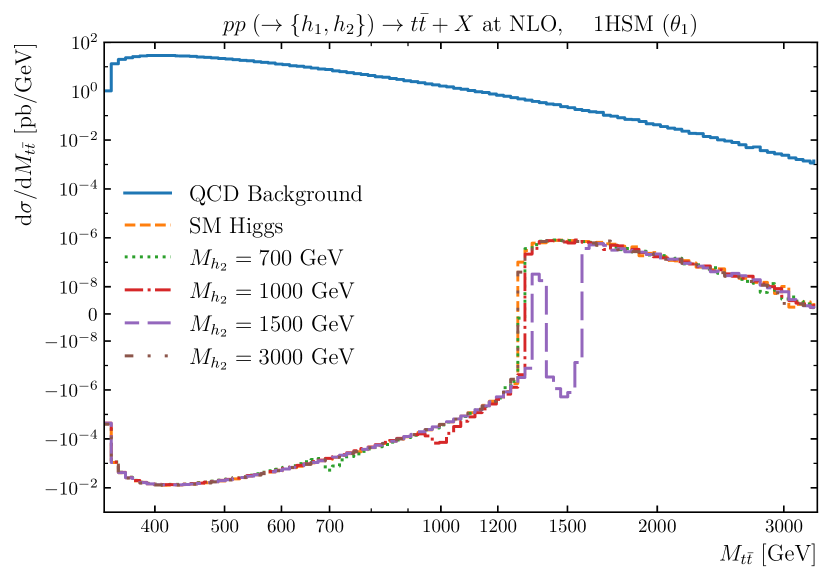
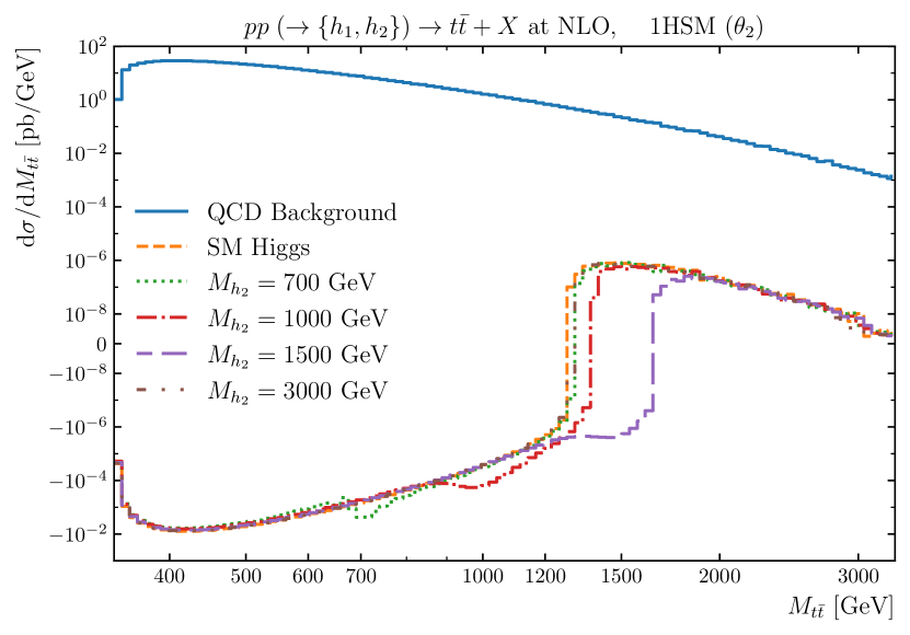
Figure 6: NLO differential distribution in $M_{t\bar{t}}$ for the QCD continuum $pp\to t\bar{t}+X$, the SM Higgs mediated process $pp\,(\to h)\to t\bar{t}+X$ and the BSM process $pp\,(\to h_{1},h_{2})\to t\bar{t}+X$ at NLO in the 1HSM for several benchmark scenarios with $\theta=\theta_{1}$ (upper plot) and $\theta=\theta_{1}$ (lower plot). The ${\rm d}\sigma/{\rm d}M_{t\bar{t}}$ axis is plotted in log-scale with a linearised section between $-10^{-8}$ and $10^{-8}$.

We consider distributions in the invariant mass of the $t\bar{t}$ system, $M_{t\bar{t}}$, for the SM and the BSM benchmark scenarios of table 1. In figure 6, we plot the corresponding NLO differential distributions for $\theta=\theta_{1}$ (upper plot) and $\theta=\theta_{2}$ (lower plot) over a large mass range. In each figure we separate the relevant contributions according to eq. (13), namely the QCD background ($\left|\mathcal{M}_{\text{QCD}}\right|^{2}$), the SM Higgs contributions ($\left|\mathcal{M}_{h_{1}}\right|^{2}+2\,\mathrm{Re}(\mathcal{M}_{h_{1}}^{\ast}\mathcal{M}_{\text{QCD}})$) and the SM+BSM Higgs contributions ($\left|\mathcal{M}_{h_{1}}\right|^{2}+\left|\mathcal{M}_{h_{2}}\right|^{2}+2\,\mathrm{Re}\left(\left(\mathcal{M}_{h_{1}}^{\ast}+\mathcal{M}_{h_{2}}^{\ast}\right)\mathcal{M}_{\text{QCD}}\right)+2\,\mathrm{Re}(\mathcal{M}_{h_{1}}^{\ast}\mathcal{M}_{h_{2}}^{\ast})$). The latter are labelled according to the value of the mass of the heavy Higgs. The Higgs contributions are suppressed by about two orders of magnitude with respect to the QCD background. The BSM contributions largely follow the SM continuum apart from the peak/dip structure around the mass of the heavy Higgs. A precise modelling of these structures is crucial in order to separate the overwhelming QCD background. The SM Higgs and the BSM Higgs predictions are largely dominated by the interference contributions yielding negative cross-sections up to $M_{t\bar{t}}\approx 1300$ GeV. The SM Higgs contribution turns positive at around $M_{t\bar{t}}\approx 1300$ GeV yielding a spurious enhanced shape in the chosen linearised log plot for all SM Higgs and BSM Higgs predictions. We note that for $\theta=\theta_{2}$ the deviations around the mass of the heavy Higgs are smeared out compared to those for $\theta=\theta_{1}$. This is expected as the width of the resonances for $\theta=\theta_{2}$ are larger than for $\theta=\theta_{1}$, as listed in table 2. The peak/dip structure for the BSM scenario with $M_{h_{2}}=3000$ GeV is marginally visible in these plots and we will neglect it in the further discussion. Such high masses of the heavy Higgs will be out-of-reach even at the HL-LHC.

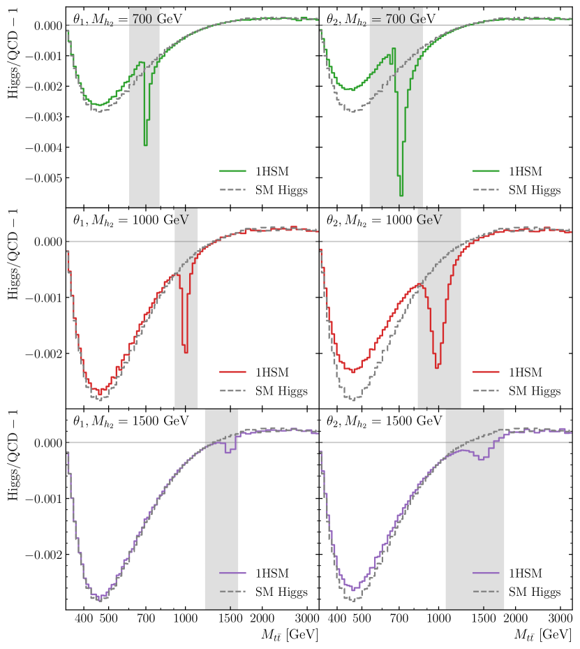
Figure 7: Relative difference Higgs/QCD$-1$ of the Higgs contribution (signal and interference) for the process $pp\,(\to\{h_{1},h_{2}\})\to t\bar{t}+X$ with respect to the continuum QCD background at NLO differential in the top-pair invariant mass, $M_{t\bar{t}}$, for each 1HSM benchmark point and in the SM. The chosen invariant mass windows are represented by a grey band.

In order to highlight the peak/dip structure in the BSM scenarios in more detail, which is the key objective of the paper at hand, in figure 7 we consider again the NLO differential distribution in $M_{t\bar{t}}$ showing the relative difference between the (B)SM Higgs predictions in the 1HSM/SM and the QCD continuum, labelled $\rm{Higgs/QCD}-1$. A corresponding plot differential in the average transverse momentum of the top and anti-top quark is shown in appendix B. For all benchmark points the BSM effects manifest as a rather sharp dip around the heavy Higgs mass on top of the SM Higgs continuum. This dip is significantly wider in the case of $\theta=\theta_{2}$ due to the increased heavy Higgs widths. Additionally, for $\theta=\theta_{2}$ there are significant $h_{1}$-$h_{2}$ and off-shell $h_{2}$-QCD interference effects which alter the shape of the Higgs continuum even away from the resonance region. At the negative maximum of the relative contribution of the Higgs continuum at around $M_{t\bar{t}}\approx 450$ GeV these interference effects yield a relative reduction of around $30\%$. Based on the shapes of the dip structures around the resonance regions we select suitable invariant mass windows for each benchmark point around the resonance structures. These invariant mass windows are highlighted as grey bands in figure 7 and listed in table 4. Within these invariant windows in figure 8 we zoom into the respective differential distributions in the top-pair invariant mass and show absolute NLO and LO predictions for the SM and BSM processes $pp\,(\to h_{1},h_{2})\to t\bar{t}+X$ for all considered benchmark points. NLO corrections are large reaching more than 100% and typically broaden the resonance dip towards larger invariant masses. The shown uncertainty bands at NLO are obtained from renormalisation and factorisation scale variations based on the envelope of a seven-point variation around the central scale choice in eq. (16), i.e. considering the combinations $(\mu_{R},\mu_{F})=(2\mu,2\mu),(\mu/2,\mu/2),(2\mu,\mu),\allowbreak(\mu/2,\mu),(\mu,2\mu),(\mu,\mu/2)$. Scale uncertainties are at the level of $20-30\%$ in the resonance regions. We checked that these NLO uncertainty bands do not overlap with corresponding bands at LO (not shown). Due to the large higher-order corrections affecting the processes at hand NLO is the first perturbative order where a reliable estimate of theoretical uncertainties can be inferred from scale variation. In all invariant mass windows NLO corrections and uncertainties at NLO increase towards smaller invariant masses. This can be understood from a shift of events from the resonance region to invariant masses above and below the resonance, and the steepness of the corresponding differential distribution.

Invariant $M_{h_{2}}$ [GeV] mass window $\theta_{1}$ $700$ $600$–$790$ GeV $1000$ $900$–$1115$ GeV $1500$ $1200$–$1600$ GeV $\theta_{2}$ $700$ $530$–$870$ GeV $1000$ $830$–$1200$ GeV $1500$ $1050$–$1800$ GeV

Table 4: The 1HSM benchmark points that may be excluded at a $95\%$ confidence level in the corresponding data samples for the LHC Run 2 and the future Run 3 and HL-LHC.

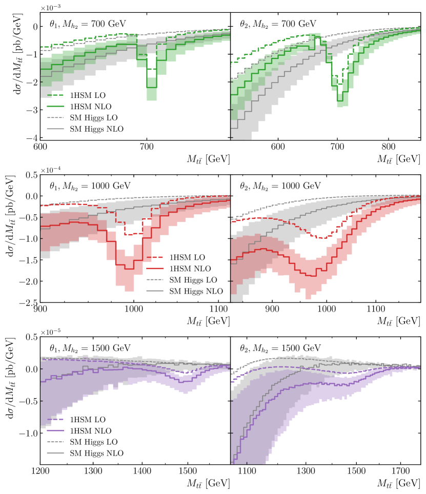
Figure 8: Differential distributions in $M_{t\bar{t}}$ for the combined Higgs contribution (signal and interference) in the 1HSM and in the SM to the process $pp\,(\to\{h_{1},h_{2}\})\to t\bar{t}+X$ comparing NLO (solid) and LO (dashed) predictions for each benchmark point in the respective invariant mass window as defined in table 4.

5.3 Sensitivity estimates to BSM effects

Invariant Excludable $M_{h_{2}}$ [GeV] mass window Run 2 Run 3 HL-LHC $\theta_{1}$ $700$ $600$–$790$ GeV ✓ ✓ ✓ $1000$ $900$–$1115$ GeV – ✓ ✓ $1500$ $1200$–$1600$ GeV – – – $\theta_{2}$ $700$ $530$–$870$ GeV ✓ ✓ ✓ $1000$ $830$–$1200$ GeV ✓ ✓ ✓ $1500$ $1050$–$1800$ GeV – – –

Table 5: The 1HSM benchmark points that may be excluded at a $95\%$ confidence level in the corresponding data samples for the LHC Run 2 and the future Run 3 and HL-LHC.

Based on the obtained NLO cross sections for the 1HSM benchmarks we can estimate the sensitivity of current and future LHC runs in excluding these BSM scenarios. Within each invariant mass window as defined in table 4 we consider $|S|/\sqrt{B}=\sqrt{\mathcal{L}}\,|\sigma_{S}|/\sqrt{\sigma_{B}}$ as a naive estimate for the significance from Poisson statistics Barlow:1993 , where $\sigma_{S}$ and $\sigma_{B}$ are the cross sections integrated over the appropriate $M_{t\bar{t}}$ window, and $\mathcal{L}$ is the integrated luminosity of the considered LHC scenario. In particular, we consider the full LHC Run 2 data sample corresponding to an integrated luminosity of $\mathcal{L}=139\text{ fb}^{-1}$ ATLAS:2019pzw , the projected integrated luminosity for LHC Run 3 of $\mathcal{L}\approx 300\text{ fb}^{-1}$, and of $\mathcal{L}\approx 3000\text{ fb}^{-1}$ for the future high luminosity (HL-LHC) upgrade ZurbanoFernandez:2020cco . As signal cross section $\sigma_{S}$ we consider the entire Higgs contribution including $h_{1}$ and $h_{2}$ (and their interference) and the Higgs-QCD interference. As background $\sigma_{B}$ we consider the QCD continuum. The fiducial cross sections for the Higgs signals are mostly negative due to sizable Higgs-QCD interferences. Therefore we pragmatically consider the absolute value in the significance estimate.

We consider a benchmark point to be excludable if $|S|/\sqrt{B}>2$. However, this can only be seen as a simplified estimate, since we do not take into account either top decays, phase space cuts, or experimental systematics. We find that purely based on statistical uncertainties benchmark points with $M_{h_{2}}=700$ GeV could be excluded already from Run 2 alone. For benchmark points with $M_{h_{2}}=1000$ GeV, these may be excluded from Run 3 or HL-LHC data for $\theta=\theta_{2}$ but only from HL-LHC data for $\theta=\theta_{2}$. Benchmark points with $M_{h_{2}}=1500$ GeV cannot be excluded in any of the three scenarios and thus will not be excluded in any practical LHC set-up. In order to test such scenarios future collider projects like the FCC-hh are essential.

6 Conclusion

In this work we considered the 1-Higgs-singlet extension of the SM including an additional heavy Higgs that can decay into a $t\bar{t}$ pair. The production of such a particle interferes with QCD $t\bar{t}$ production, and it is possible that the interference pattern leads to appreciable modifications of physical cross sections, for instance in the differential distribution in $M_{t\bar{t}}$, the invariant mass of the $t\bar{t}$ pair. Extending the analysis of ref. Kauer:2019qei , we have computed the full set of NLO corrections to the production of a scalar decaying into a $t\bar{t}$ pair, for the case of stable top quarks. The corrections entail at the virtual level two-loop amplitudes containing Higgs bosons in interference with the QCD background at tree-level and one-loop Higgs boson amplitudes in interference with the one-loop QCD background, and corresponding loop-squared amplitudes at the real radiation level. The two-loop amplitudes containing Higgs bosons can be separated into “factorisable” and “non-factorisable”. Factorisable two-loop diagrams are computed exactly, while the non-factorisable two-loop contributions which are beyond today’s loop technology, are included in such a way as to preserve all singular limits. The ingredients of such a calculation are not available in current automated tools. Therefore, we built our own Monte Carlo framework by acquiring amplitudes from a modified OpenLoops 2, using the dipole subtraction implementation from Helac-Dipoles, and Kaleu for phase-space integration. In this framework factorisable two-loop corrections are included via appropriate form-factors inserted into OpenLoops tree amplitudes.

In our numerical analysis we found that the presence of an additional Higgs boson induces distinct features in the $M_{t\bar{t}}$ distribution, located around the mass of the heavy Higgs. These features are affected by large NLO corrections, which broaden the $M_{t\bar{t}}$ distribution relative to the LO one. Performing a scan in $M_{t\bar{t}}$, we were able to find windows where it may be possible to exclude some parameters of the considered BSM model with the current and future runs of the LHC. But in order to draw definite conclusions, one needs to upgrade our calculation to include top decays, and apply realistic experimental cuts. It would also be desirable to identify alternative observables to $M_{t\bar{t}}$ that show the same degree of sensitivity to BSM effects, but are less affected by real QCD radiation. We leave both questions to future work. In summary, this study provides the key ingredients to assess the impact of interference effects in BSM searches at NLO accuracy. The developed Helac+OpenLoop Monte Carlo program for the computation of $pp\;(\to\{h_{1},h_{2}\})\to t\bar{t}+X$ in the SM and the 1HSM is available upon request.

Appendix A Decays of the heavy Higgs in the 1HSM

$\theta=\theta_{1}$ $M_{h_{2}}$ [GeV] $\Gamma\left(h_{2}\to 2\times h_{1}\right)$ [GeV] $\Gamma\left(h_{2}\to 3\times h_{1}\right)$ [GeV] $\Gamma\left(h_{2}\to 4\times h_{1}\right)$ [GeV] $700$ $2.1556(1)$ $0.00468(2)$ $6.24(4)\times 10^{-7}$ $1000$ $6.0953(1)$ $0.1692(7)$ $0.001718(9)$ $1500$ $9.8911(1)$ $0.218(2)$ $0.001632(8)$ $3000$ $20.658(1)$ $0.306(2)$ $0.001060(7)$ $\theta=\theta_{2}$ $M_{h_{2}}$ [GeV] $\Gamma\left(h_{2}\to 2\times h_{1}\right)$ [GeV] $\Gamma\left(h_{2}\to 3\times h_{1}\right)$ [GeV] $\Gamma\left(h_{2}\to 4\times h_{1}\right)$ [GeV] $700$ $4.1798(1)$ $0.507(2)$ $0.01451(8)$ $1000$ $11.604(1)$ $7.34(4)$ $2.46(2)$ $1500$ $27.26(1)$ $12.9(2)$ $3.91(2)$ $3000$ $66.8(1)$ $21.4(2)$ $4.17(2)$

Table 6: Partial decay widths for $h_{2}\to n\times h_{1}$ for $n=2,3,$ and $4$ in the 1HSM for the eight different benchmark points.

As detailed in section 4.2 we determine the widths of the light and heavy Higgs bosons in the 1HSM as

$$\Gamma_{h_{1}} =\Gamma_{H}\!\left(M_{h_{1}}\right)\cos^{2}\theta\,,$$ (25)

$$\Gamma_{h_{2}} =\Gamma_{H}\!\left(M_{h_{2}}\right)\sin^{2}\theta+\Gamma\!\left(h_{2}\rightarrow n\times h_{1}\right)\,,$$ (26)

where $\Gamma_{H}(M)$ refers to the decay width of a SM Higgs with mass $M$, and $\Gamma\left(h_{2}\rightarrow n\times h_{1}\right)$ to the partial decay widths for the heavy scalar $h_{2}$ decaying into $n$ light scalars. We compute and include this latter partial decay width for $2\leq n\leq 4$. A custom implementation of the 1HSM in FeynRules Alloul:2013bka ; Christensen:2008py was used to produce a UFO Degrande:2011ua implementation that was subsequently used in MadGraph5_aMC@NLO Alwall:2014hca to calculate the partial decay widths $\Gamma\left(h_{2}\rightarrow n\times h_{1}\right)$, the results of which are shown in table 6. It is clear that partial decay widths for decays to higher multiplicities, $n>4$, of $h_{1}$ are suppressed. The partial decay widths for $n>2$ is due to cascaded emissions of $h_{2}\to h_{2}h_{1}$ and decays $h_{2}\to h_{1}h_{1}$, as illustrated in figure 9.

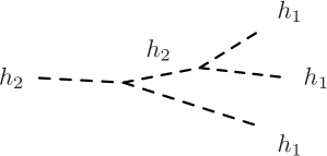
Figure 9: The cascaded partial decay of $h_{2}\to 3\times h_{1}$.

The computation of the decay width $\Gamma_{h_{2}}$ implies a circular dependence due to the regularisation of the $h_{2}$ propagator via $\Gamma_{h_{2}}$ itself. This is not problematic if $\Gamma_{h_{2}}/M_{h_{2}}\ll 1$, but as can be seen in table 2 one of the benchmark points reaches $\Gamma_{h_{2}}/M_{h_{2}}\sim 0.18$. A simple solution would be to recursively calculate the decay width. However, in the case of $\Gamma/M\sim 1$ the Breit-Wigner approximation does not hold, and one should use a better estimate of the self energy $\Sigma(p^{2})$ in the exact propagator expression. It is important, however, to do this in a gauge-invariant way. This would likely produce a tiny correction in this case, and has therefore not been done in this study. But it may be necessary for certain new physics models that introduces resonances with large decay widths.

Appendix B Additional differential distributions

In this appendix we include additional differential distributions for the process $pp\,(\to h_{1},h_{2})\to t\bar{t}+X$ in the 1HSM. In figure 10 we show differential distributions in the average $p_{T}$ of the $t$ and $\bar{t}$, $p_{T,\text{average}}=(p_{T,t}+p_{T,\bar{t}})/2$, for each 1HSM benchmark point normalised to the QCD continuum.

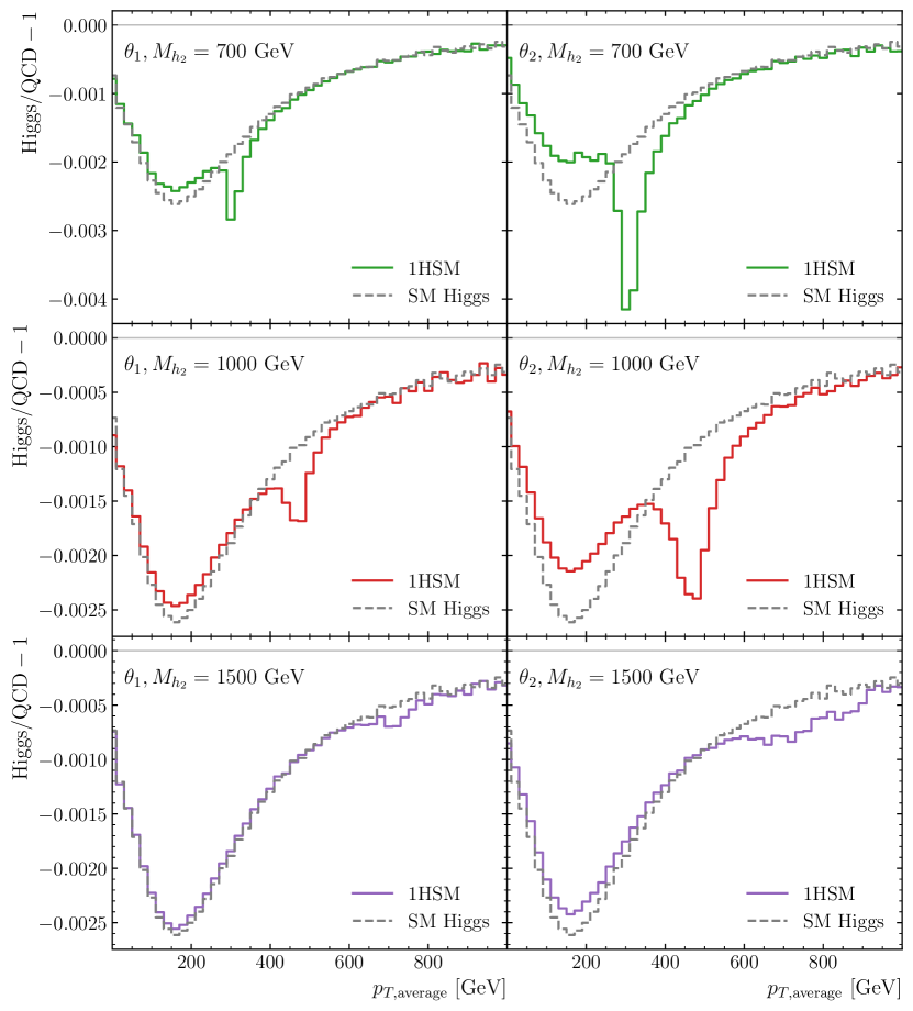
Figure 10: Relative difference Higgs/QCD$-1$ of the Higgs contribution (signal and interference) for the process $pp\,(\to\{h_{1},h_{2}\})\to t\bar{t}+X$ with respect to the continuum QCD background at NLO differential in $p_{T,\text{average}}$, for each 1HSM benchmark point and in the SM.

References

- (1) ATLAS collaboration, Observation of a new particle in the search for the Standard Model Higgs boson with the ATLAS detector at the LHC, Phys. Lett. B 716 (2012) 1 [1207.7214].
- (2) CMS collaboration, Observation of a New Boson at a Mass of 125 GeV with the CMS Experiment at the LHC, Phys. Lett. B 716 (2012) 30 [1207.7235].
- (3) P. Higgs, Broken symmetries, massless particles and gauge fields, Physics Letters 12 (1964) 132.
- (4) P.W. Higgs, Broken symmetries and the masses of gauge bosons, Phys. Rev. Lett. 13 (1964) 508.
- (5) P.W. Higgs, Spontaneous symmetry breakdown without massless bosons, Phys. Rev. 145 (1966) 1156.
- (6) F. Englert and R. Brout, Broken symmetry and the mass of gauge vector mesons, Phys. Rev. Lett. 13 (1964) 321.
- (7) G.S. Guralnik, C.R. Hagen and T.W.B. Kibble, Global conservation laws and massless particles, Phys. Rev. Lett. 13 (1964) 585.
- (8) S. Profumo, M.J. Ramsey-Musolf, C.L. Wainwright and P. Winslow, Singlet-catalyzed electroweak phase transitions and precision Higgs boson studies, Phys. Rev. D 91 (2015) 035018 [1407.5342].
- (9) A. Papaefstathiou and G. White, The electro-weak phase transition at colliders: confronting theoretical uncertainties and complementary channels, JHEP 05 (2021) 099 [2010.00597].
- (10) A. Papaefstathiou and G. White, The Electro-Weak Phase Transition at Colliders: Discovery Post-Mortem, JHEP 02 (2022) 185 [2108.11394].
- (11) D. Gonçalves, A. Kaladharan and Y. Wu, Resonant top pair searches at the LHC: A window to the electroweak phase transition, Phys. Rev. D 107 (2023) 075040 [2206.08381].
- (12) T. Binoth and J.J. van der Bij, Influence of strongly coupled, hidden scalars on Higgs signals, Z. Phys. C 75 (1997) 17 [hep-ph/9608245].
- (13) R.M. Schabinger and J.D. Wells, A Minimal spontaneously broken hidden sector and its impact on Higgs boson physics at the large hadron collider, Phys. Rev. D 72 (2005) 093007 [hep-ph/0509209].
- (14) B. Patt and F. Wilczek, Higgs-field portal into hidden sectors, hep-ph/0605188.
- (15) M. Bowen, Y. Cui and J.D. Wells, Narrow trans-TeV Higgs bosons and H — hh decays: Two LHC search paths for a hidden sector Higgs boson, JHEP 03 (2007) 036 [hep-ph/0701035].
- (16) V. Barger, P. Langacker, M. McCaskey, M.J. Ramsey-Musolf and G. Shaughnessy, LHC Phenomenology of an Extended Standard Model with a Real Scalar Singlet, Phys. Rev. D 77 (2008) 035005 [0706.4311].
- (17) V. Barger, P. Langacker, M. McCaskey, M. Ramsey-Musolf and G. Shaughnessy, Complex Singlet Extension of the Standard Model, Phys. Rev. D 79 (2009) 015018 [0811.0393].
- (18) G. Bhattacharyya, G.C. Branco and S. Nandi, Universal Doublet-Singlet Higgs Couplings and phenomenology at the CERN Large Hadron Collider, Phys. Rev. D 77 (2008) 117701 [0712.2693].
- (19) S. Dawson and W. Yan, Hiding the Higgs Boson with Multiple Scalars, Phys. Rev. D 79 (2009) 095002 [0904.2005].
- (20) S. Bock, R. Lafaye, T. Plehn, M. Rauch, D. Zerwas and P.M. Zerwas, Measuring Hidden Higgs and Strongly-Interacting Higgs Scenarios, Phys. Lett. B 694 (2011) 44 [1007.2645].
- (21) P.J. Fox, D. Tucker-Smith and N. Weiner, Higgs friends and counterfeits at hadron colliders, JHEP 06 (2011) 127 [1104.5450].
- (22) C. Englert, T. Plehn, D. Zerwas and P.M. Zerwas, Exploring the Higgs portal, Phys. Lett. B 703 (2011) 298 [1106.3097].
- (23) C. Englert, J. Jaeckel, E. Re and M. Spannowsky, Evasive Higgs Maneuvers at the LHC, Phys. Rev. D 85 (2012) 035008 [1111.1719].
- (24) B. Batell, S. Gori and L.-T. Wang, Exploring the Higgs Portal with 10/fb at the LHC, JHEP 06 (2012) 172 [1112.5180].
- (25) C. Englert, T. Plehn, M. Rauch, D. Zerwas and P.M. Zerwas, LHC: Standard Higgs and Hidden Higgs, Phys. Lett. B 707 (2012) 512 [1112.3007].
- (26) R.S. Gupta and J.D. Wells, Higgs boson search significance deformations due to mixed-in scalars, Phys. Lett. B 710 (2012) 154 [1110.0824].
- (27) M.J. Dolan, C. Englert and M. Spannowsky, New Physics in LHC Higgs boson pair production, Phys. Rev. D 87 (2013) 055002 [1210.8166].
- (28) B. Batell, D. McKeen and M. Pospelov, Singlet Neighbors of the Higgs Boson, JHEP 10 (2012) 104 [1207.6252].
- (29) J.M. No and M. Ramsey-Musolf, Probing the Higgs Portal at the LHC Through Resonant di-Higgs Production, Phys. Rev. D 89 (2014) 095031 [1310.6035].
- (30) R. Coimbra, M.O.P. Sampaio and R. Santos, ScannerS: Constraining the phase diagram of a complex scalar singlet at the LHC, Eur. Phys. J. C 73 (2013) 2428 [1301.2599].
- (31) H.E. Logan, Hiding a higgs width enhancement from off-shell measurements, Phys. Rev. D 92 (2015) 075038.
- (32) C.-Y. Chen, S. Dawson and I.M. Lewis, Exploring resonant di-Higgs boson production in the Higgs singlet model, Phys. Rev. D 91 (2015) 035015 [1410.5488].
- (33) R. Costa, A.P. Morais, M.O.P. Sampaio and R. Santos, Two-loop stability of a complex singlet extended Standard Model, Phys. Rev. D 92 (2015) 025024 [1411.4048].
- (34) A. Falkowski, C. Gross and O. Lebedev, A second Higgs from the Higgs portal, JHEP 05 (2015) 057 [1502.01361].
- (35) V. Martín Lozano, J.M. Moreno and C.B. Park, Resonant Higgs boson pair production in the decay channel, JHEP 08 (2015) 004 [1501.03799].
- (36) S. Kanemura, M. Kikuchi and K. Yagyu, Radiative corrections to the Higgs boson couplings in the model with an additional real singlet scalar field, Nucl. Phys. B 907 (2016) 286 [1511.06211].
- (37) S. Kanemura, M. Kikuchi and K. Yagyu, One-loop corrections to the Higgs self-couplings in the singlet extension, Nucl. Phys. B 917 (2017) 154 [1608.01582].
- (38) S. Kanemura, M. Kikuchi, K. Sakurai and K. Yagyu, H-COUP: a program for one-loop corrected Higgs boson couplings in non-minimal Higgs sectors, Comput. Phys. Commun. 233 (2018) 134 [1710.04603].
- (39) I.M. Lewis and M. Sullivan, Benchmarks for Double Higgs Production in the Singlet Extended Standard Model at the LHC, Phys. Rev. D 96 (2017) 035037 [1701.08774].
- (40) J.A. Casas, D.G. Cerdeño, J.M. Moreno and J. Quilis, Reopening the Higgs portal for single scalar dark matter, JHEP 05 (2017) 036 [1701.08134].
- (41) L. Altenkamp, M. Boggia and S. Dittmaier, Precision calculations for fermions in a Singlet Extension of the Standard Model with Prophecy4f, JHEP 04 (2018) 062 [1801.07291].
- (42) H. Abouabid, A. Arhrib, D. Azevedo, J.E. Falaki, P.M. Ferreira, M. Mühlleitner et al., Benchmarking di-Higgs production in various extended Higgs sector models, JHEP 09 (2022) 011 [2112.12515].
- (43) G.M. Pruna and T. Robens, Higgs singlet extension parameter space in the light of the LHC discovery, Phys. Rev. D 88 (2013) 115012 [1303.1150].
- (44) T. Robens and T. Stefaniak, Status of the Higgs Singlet Extension of the Standard Model after LHC Run 1, Eur. Phys. J. C 75 (2015) 104 [1501.02234].
- (45) T. Robens and T. Stefaniak, LHC Benchmark Scenarios for the Real Higgs Singlet Extension of the Standard Model, Eur. Phys. J. C 76 (2016) 268 [1601.07880].
- (46) A. Ilnicka, T. Robens and T. Stefaniak, Constraining Extended Scalar Sectors at the LHC and beyond, Mod. Phys. Lett. A 33 (2018) 1830007 [1803.03594].
- (47) J. Alison et al., Higgs boson potential at colliders: Status and perspectives, Rev. Phys. 5 (2020) 100045 [1910.00012].
- (48) ATLAS collaboration, Search for Higgs boson pair production in the two bottom quarks plus two photons final state in collisions at TeV with the ATLAS detector, Phys. Rev. D 106 (2022) 052001 [2112.11876].
- (49) ATLAS collaboration, Search for resonant pair production of Higgs bosons in the final state using collisions at = 13 TeV with the ATLAS detector, Phys. Rev. D 105 (2022) 092002 [2202.07288].
- (50) K.J.F. Gaemers and F. Hoogeveen, Higgs Production and Decay Into Heavy Flavors With the Gluon Fusion Mechanism, Phys. Lett. B 146 (1984) 347.
- (51) D. Dicus, A. Stange and S. Willenbrock, Higgs decay to top quarks at hadron colliders, Phys. Lett. B 333 (1994) 126 [hep-ph/9404359].
- (52) R. Frederix and F. Maltoni, Top pair invariant mass distribution: A Window on new physics, JHEP 01 (2009) 047 [0712.2355].
- (53) S. Jung, J. Song and Y.W. Yoon, Dip or nothingness of a Higgs resonance from the interference with a complex phase, Phys. Rev. D 92 (2015) 055009 [1505.00291].
- (54) A. Djouadi, J. Ellis and J. Quevillon, Interference effects in the decays of spin-zero resonances into and , JHEP 07 (2016) 105 [1605.00542].
- (55) S. Gori, I.-W. Kim, N.R. Shah and K.M. Zurek, Closing the Wedge: Search Strategies for Extended Higgs Sectors with Heavy Flavor Final States, Phys. Rev. D 93 (2016) 075038 [1602.02782].
- (56) M. Carena and Z. Liu, Challenges and opportunities for heavy scalar searches in the channel at the LHC, JHEP 11 (2016) 159 [1608.07282].
- (57) M. Czakon, D. Heymes and A. Mitov, Bump hunting in LHC events, Phys. Rev. D 94 (2016) 114033 [1608.00765].
- (58) W. Bernreuther, P. Galler, C. Mellein, Z.G. Si and P. Uwer, Production of heavy Higgs bosons and decay into top quarks at the LHC, Phys. Rev. D 93 (2016) 034032 [1511.05584].
- (59) B. Hespel, F. Maltoni and E. Vryonidou, Signal background interference effects in heavy scalar production and decay to a top-anti-top pair, JHEP 10 (2016) 016 [1606.04149].
- (60) W. Bernreuther, P. Galler, Z.-G. Si and P. Uwer, Production of heavy Higgs bosons and decay into top quarks at the LHC. II: Top-quark polarization and spin correlation effects, Phys. Rev. D 95 (2017) 095012 [1702.06063].
- (61) D. Buarque Franzosi, E. Vryonidou and C. Zhang, Scalar production and decay to top quarks including interference effects at NLO in QCD in an EFT approach, JHEP 10 (2017) 096 [1707.06760].
- (62) D. Buarque Franzosi, F. Fabbri and S. Schumann, Constraining scalar resonances with top-quark pair production at the LHC, JHEP 03 (2018) 022 [1711.00102].
- (63) P. Basler, S. Dawson, C. Englert and M. Mühlleitner, Di-Higgs boson peaks and top valleys: Interference effects in Higgs sector extensions, Phys. Rev. D 101 (2020) 015019 [1909.09987].
- (64) A. Djouadi, J. Ellis, A. Popov and J. Quevillon, Interference effects in production at the LHC as a window on new physics, JHEP 03 (2019) 119 [1901.03417].
- (65) N. Kauer, A. Lind, P. Maierhöfer and W. Song, Higgs interference effects at the one-loop level in the 1-Higgs-Singlet extension of the Standard Model, JHEP 07 (2019) 108 [1905.03296].
- (66) S. Frixione, L. Roos, E. Ting, E. Vryonidou, M. White and A.G. Williams, Model-independent approach for incorporating interference effects in collider searches for new resonances, Eur. Phys. J. C 80 (2020) 1174 [2008.07751].
- (67) O. Atkinson, C. Englert and P. Stylianou, On interference effects in top-philic decay chains, Phys. Lett. B 821 (2021) 136618 [2012.07424].
- (68) LHC Higgs Cross Section Working Group collaboration, Handbook of LHC Higgs Cross Sections: 3. Higgs Properties, 1307.1347.
- (69) P. Nason, S. Dawson and R.K. Ellis, The Total Cross-Section for the Production of Heavy Quarks in Hadronic Collisions, Nucl. Phys. B 303 (1988) 607.
- (70) W. Beenakker, H. Kuijf, W.L. van Neerven and J. Smith, QCD Corrections to Heavy Quark Production in p anti-p Collisions, Phys. Rev. D 40 (1989) 54.
- (71) W. Beenakker, W.L. van Neerven, R. Meng, G.A. Schuler and J. Smith, QCD corrections to heavy quark production in hadron hadron collisions, Nucl. Phys. B 351 (1991) 507.
- (72) M.L. Mangano, P. Nason and G. Ridolfi, Heavy quark correlations in hadron collisions at next-to-leading order, Nucl. Phys. B 373 (1992) 295.
- (73) P. Bärnreuther, M. Czakon and A. Mitov, Percent Level Precision Physics at the Tevatron: First Genuine NNLO QCD Corrections to , Phys. Rev. Lett. 109 (2012) 132001 [1204.5201].
- (74) M. Czakon and A. Mitov, NNLO corrections to top-pair production at hadron colliders: the all-fermionic scattering channels, JHEP 12 (2012) 054 [1207.0236].
- (75) M. Czakon and A. Mitov, NNLO corrections to top pair production at hadron colliders: the quark-gluon reaction, JHEP 01 (2013) 080 [1210.6832].
- (76) M. Czakon, P. Fiedler and A. Mitov, Total Top-Quark Pair-Production Cross Section at Hadron Colliders Through , Phys. Rev. Lett. 110 (2013) 252004 [1303.6254].
- (77) M. Czakon, D. Heymes and A. Mitov, High-precision differential predictions for top-quark pairs at the LHC, Phys. Rev. Lett. 116 (2016) 082003 [1511.00549].
- (78) M. Czakon, P. Fiedler, D. Heymes and A. Mitov, NNLO QCD predictions for fully-differential top-quark pair production at the Tevatron, JHEP 05 (2016) 034 [1601.05375].
- (79) S. Catani, S. Devoto, M. Grazzini, S. Kallweit and J. Mazzitelli, Top-quark pair production at the LHC: Fully differential QCD predictions at NNLO, JHEP 07 (2019) 100 [1906.06535].
- (80) S. Catani, S. Devoto, M. Grazzini, S. Kallweit, J. Mazzitelli and H. Sargsyan, Top-quark pair hadroproduction at next-to-next-to-leading order in QCD, Phys. Rev. D 99 (2019) 051501 [1901.04005].
- (81) R. Harlander and P. Kant, Higgs production and decay: Analytic results at next-to-leading order QCD, JHEP 12 (2005) 015 [hep-ph/0509189].
- (82) A. van Hameren, Kaleu: A General-Purpose Parton-Level Phase Space Generator, 1003.4953.
- (83) S. Catani and M.H. Seymour, A General algorithm for calculating jet cross-sections in NLO QCD, Nucl. Phys. B 485 (1997) 291 [hep-ph/9605323].
- (84) S. Catani, S. Dittmaier, M.H. Seymour and Z. Trocsanyi, The Dipole formalism for next-to-leading order QCD calculations with massive partons, Nucl. Phys. B 627 (2002) 189 [hep-ph/0201036].
- (85) M. Czakon, C.G. Papadopoulos and M. Worek, Polarizing the Dipoles, JHEP 08 (2009) 085 [0905.0883].
- (86) F. Buccioni, J.-N. Lang, J.M. Lindert, P. Maierhöfer, S. Pozzorini, H. Zhang et al., OpenLoops 2, Eur. Phys. J. C 79 (2019) 866 [1907.13071].
- (87) S. Buehler and C. Duhr, CHAPLIN - Complex Harmonic Polylogarithms in Fortran, Comput. Phys. Commun. 185 (2014) 2703 [1106.5739].
- (88) E. Remiddi and J.A.M. Vermaseren, Harmonic polylogarithms, Int. J. Mod. Phys. A 15 (2000) 725 [hep-ph/9905237].
- (89) J.M. Campbell and R.K. Ellis, An Update on vector boson pair production at hadron colliders, Phys. Rev. D 60 (1999) 113006 [hep-ph/9905386].
- (90) J.M. Campbell, R.K. Ellis and C. Williams, Vector boson pair production at the LHC, JHEP 07 (2011) 018 [1105.0020].
- (91) J.M. Campbell, R.K. Ellis and W.T. Giele, A Multi-Threaded Version of MCFM, Eur. Phys. J. C 75 (2015) 246 [1503.06182].
- (92) J. Campbell and T. Neumann, Precision Phenomenology with MCFM, JHEP 12 (2019) 034 [1909.09117].
- (93) R.V. Harlander, S. Liebler and H. Mantler, SusHi: A program for the calculation of Higgs production in gluon fusion and bottom-quark annihilation in the Standard Model and the MSSM, Comput. Phys. Commun. 184 (2013) 1605 [1212.3249].
- (94) R.V. Harlander, S. Liebler and H. Mantler, SusHi Bento: Beyond NNLO and the heavy-top limit, Comput. Phys. Commun. 212 (2017) 239 [1605.03190].
- (95) LHC Higgs Cross Section Working Group collaboration, Handbook of LHC Higgs Cross Sections: 4. Deciphering the Nature of the Higgs Sector, 1610.07922.
- (96) J. Butterworth et al., PDF4LHC recommendations for LHC Run II, J. Phys. G 43 (2016) 023001 [1510.03865].
- (97) A. Bredenstein, A. Denner, S. Dittmaier and M.M. Weber, Precise predictions for the Higgs-boson decay H — WW/ZZ — 4 leptons, Phys. Rev. D 74 (2006) 013004 [hep-ph/0604011].
- (98) A. Bredenstein, A. Denner, S. Dittmaier and M.M. Weber, Precision calculations for the Higgs decays H — ZZ/WW — 4 leptons, Nucl. Phys. B Proc. Suppl. 160 (2006) 131 [hep-ph/0607060].
- (99) A. Bredenstein, A. Denner, S. Dittmaier and M.M. Weber, Radiative corrections to the semileptonic and hadronic Higgs-boson decays H — W W / Z Z — 4 fermions, JHEP 02 (2007) 080 [hep-ph/0611234].
- (100) A. Djouadi, J. Kalinowski and M. Spira, HDECAY: A Program for Higgs boson decays in the standard model and its supersymmetric extension, Comput. Phys. Commun. 108 (1998) 56 [hep-ph/9704448].
- (101) A. Djouadi, J. Kalinowski, M. Muehlleitner and M. Spira, HDECAY: Twenty++ years after, Comput. Phys. Commun. 238 (2019) 214 [1801.09506].
- (102) M. Spira, A. Djouadi, D. Graudenz and P.M. Zerwas, Higgs boson production at the LHC, Nucl. Phys. B 453 (1995) 17 [hep-ph/9504378].
- (103) A. Banfi, F. Caola, F.A. Dreyer, P.F. Monni, G.P. Salam, G. Zanderighi et al., Jet-vetoed Higgs cross section in gluon fusion at N3LO+NNLL with small- resummation, JHEP 04 (2016) 049 [1511.02886].
- (104) E. Bagnaschi, G. Degrassi, P. Slavich and A. Vicini, Higgs production via gluon fusion in the POWHEG approach in the SM and in the MSSM, JHEP 02 (2012) 088 [1111.2854].
- (105) P. Nason, A New method for combining NLO QCD with shower Monte Carlo algorithms, JHEP 11 (2004) 040 [hep-ph/0409146].
- (106) S. Frixione, P. Nason and C. Oleari, Matching NLO QCD computations with Parton Shower simulations: the POWHEG method, JHEP 11 (2007) 070 [0709.2092].
- (107) S. Alioli, P. Nason, C. Oleari and E. Re, A general framework for implementing NLO calculations in shower Monte Carlo programs: the POWHEG BOX, JHEP 06 (2010) 043 [1002.2581].
- (108) J. Davies, F. Herren and M. Steinhauser, Top Quark Mass Effects in Higgs Boson Production at Four-Loop Order: Virtual Corrections, Phys. Rev. Lett. 124 (2020) 112002 [1911.10214].
- (109) U. Aglietti, R. Bonciani, G. Degrassi and A. Vicini, Analytic Results for Virtual QCD Corrections to Higgs Production and Decay, JHEP 01 (2007) 021 [hep-ph/0611266].
- (110) A. Lind and A. Banfi, H1jet, a fast program to compute transverse momentum distributions, Eur. Phys. J. C 81 (2021) 72 [2011.04694].
- (111) R.J. Barlow, Statistics: A Guide to the Use of Statistical Methods in the Physical Sciences, Wiley (12, 1993).
- (112) ATLAS collaboration, Luminosity determination in collisions at TeV using the ATLAS detector at the LHC, .
- (113) I. Zurbano Fernandez et al., High-Luminosity Large Hadron Collider (HL-LHC): Technical design report, .
- (114) A. Alloul, N.D. Christensen, C. Degrande, C. Duhr and B. Fuks, FeynRules 2.0 - A complete toolbox for tree-level phenomenology, Comput. Phys. Commun. 185 (2014) 2250 [1310.1921].
- (115) N.D. Christensen and C. Duhr, FeynRules - Feynman rules made easy, Comput. Phys. Commun. 180 (2009) 1614 [0806.4194].
- (116) C. Degrande, C. Duhr, B. Fuks, D. Grellscheid, O. Mattelaer and T. Reiter, UFO - The Universal FeynRules Output, Comput. Phys. Commun. 183 (2012) 1201 [1108.2040].
- (117) J. Alwall, R. Frederix, S. Frixione, V. Hirschi, F. Maltoni, O. Mattelaer et al., The automated computation of tree-level and next-to-leading order differential cross sections, and their matching to parton shower simulations, JHEP 07 (2014) 079 [1405.0301].