Evidence of a Cloud-Cloud Collision from Overshooting Gas in the Galactic Center

Abstract

The Milky Way is a barred spiral galaxy with “bar lanes” that bring gas towards the Galactic Center. Gas flowing along these bar lanes often overshoots, and instead of accreting onto the Central Molecular Zone, it collides with the bar lane on the opposite side of the Galaxy. We observed G5, a cloud which we believe is the site of one such collision, near the Galactic Center at $(\ell,b)=(+5.4,-0.4)$ with the ALMA/ACA. We took measurements of the spectral lines ^12CO $J=2\shortrightarrow 1$ , ^13CO $J=2\shortrightarrow 1$ , C^18O $J=2\shortrightarrow 1$, H2CO $J=3_{03}\shortrightarrow 2_{02}$ , H2CO $J=3_{22}\shortrightarrow 2_{21}$ , CH3OH $J=4_{22}\shortrightarrow 3_{12}$ , OCS $J=18\shortrightarrow 17$ and SiO $J=5\shortrightarrow 4$. We observed a velocity bridge between two clouds at $\sim$ and $\sim$ in our position-velocity diagram, which is direct evidence of a cloud-cloud collision. We measured an average gas temperature of $\sim$$60\text{\,}\mathrm{K}$ in G5 using H2CO integrated intensity line ratios. We observed that the ^12C/^13C ratio in G5 is consistent with optically thin, or at most marginally optically thick ^12CO. We measured for the local X_CO, 10-20x less than the average Galactic value. G5 is strong direct observational evidence of gas overshooting the Central Molecular Zone (CMZ) and colliding with a bar lane on the opposite side of the Galactic center.

tablenum SIXtablenum

1 Introduction

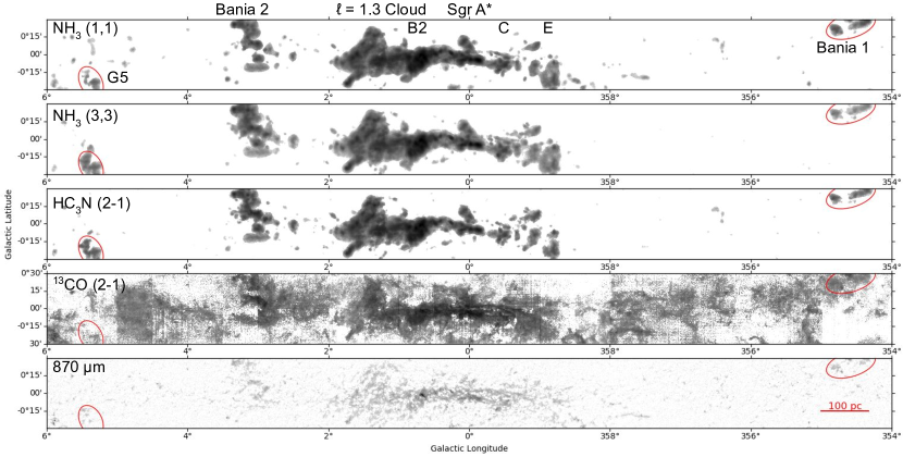
Figure 1: View of the inner $12\text{\,}\mathrm{\SIUnitSymbolDegree}$ of the Galactic plane. G5 at $(\ell,b)=(+5.4,-0.4)$ and Bania 1 at $(\ell,b)=(-5.4,+0.4)$ are circled in red. The first three panels are NH3 (1,1), NH3 (3,3) and HC3N (2-1) from the Mopra HOPS survey (hops3; hops1; hops2). The fourth panel is ^13CO (2-1) from the APEX SEDIGISM survey (SEDIGISM2021). The last panel is $850\text{\,}\micron$ from the ATLASGAL survey (atlasgal2009).

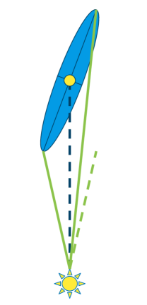
Figure 2: Geometry of the line-of-sight looking at the Milky Way’s Galactic bar, depicted as the blue ellipse bisected along its major and minor semi-axes. Not to scale. The dark blue dotted line is the line-of-sight to the center of the Galaxy, with the CMZ as the yellow ellipse. The solid green lines are lines-of-sight to the ends of the Galactic bar. The dotted green line is the same angle from the center of the Galaxy line as the solid green line to the closer end of the bar. Going by this geometry, we conclude that features at the same angular distance from the Galactic center are not necessarily related to symmetrical features on the Galactic bar.

The Milky Way is a barred spiral galaxy (blitz1991; wegg2013). It has a central, tri-axial bar. The major axis extends out to Galactocentric radii $R\sim$ $5\text{\,}\mathrm{k}\mathrm{p}\mathrm{c}$ and forms an angle with the Sun-Galactic center line of $20\text{\,}\mathrm{-}$$35\text{\,}\mathrm{\SIUnitSymbolDegree}$ (blandhawthorn2016). The bar generates a strongly non-axisymmetric gravitational potential, resulting in non-circular stellar and gaseous orbits.

At the center of the bar is the Central Molecular Zone (CMZ), host to our Galaxy’s supermassive blackhole. Figure 1 shows the inner $12\text{\,}\mathrm{\SIUnitSymbolDegree}$ of the Galactic plane in various surveys, with the CMZ at the center. The major axis of the bar is inclined relative to our line of sight, see the top down view in Figure 2, so that the near (far) end of the bar lies at positive (negative) Galactic longitudes.

The dynamics of gas in the Galactic bar can be broadly understood by considering closed periodic orbits. The two most important classes of orbits in a barred potential are X₁ and X₂ orbits (contopoulos1989). X₁ orbits are elongated with their longest axis aligned with the major axis of the Galactic bar, and can become self-intersecting at smaller radii with small cusps at both ends. X₂ orbits are ensconced within X₁ orbits at the very center of the bar. The CMZ is believed to be made of gas, dust and stars moving along X₂ orbits at the center of the Galaxy.

Gas flows along the elongated X₁ orbits while slowing drifting inwards as it loses angular momentum. At some point, the inner X₁ orbits become self-intersecting, and gas can no longer follow them, leading to the formation of large-scale shocks as the gas plunges within a dynamical time to X₂ orbits that lie much closer to the center of the Galaxy. The large-scale shocks associated with the transition between X₁ and X₂ orbits observationally correspond to the bar lanes which are observed in barred galaxies such as NGC 1300 and NGC 6782. In the Milky Way, these bar lanes have been identified in CO data cubes (fux1999; marshall2008).

Gas flows along the Galactic bar lanes at a rate that has been estimated to be $2.6\text{\,}\mathrm{M}_{\odot}\mathrm{y}\mathrm{r}^{-1}$ (sormanibarnes19). Only about a third of this gas accretes onto the CMZ, at a rate of $0.8\text{\,}\mathrm{M}_{\odot}\mathrm{y}\mathrm{r}^{-1}$ (Hatchfield2021). Note that these values are obtained assuming a Galactic-averaged X_CO factor, but as we shall see below the latter might be significantly lower in the bar lanes, leading to a lower accretion rate. The accreted gas fuels star formation in the CMZ, which is currently occuring at a rate of $0.04\text{\,}$-$0.1\text{\,}\mathrm{M}_{\odot}\mathrm{y}\mathrm{r}^{-1}$ (Yusef-Zadeh2009; Immer2012; longmore2013). The gas not accreted onto the CMZ overshoots the CMZ, eventually colliding with the bar lane on the other side of the Galaxy.

To better understand the Galactic bar, we view the inner $12\text{\,}{}^{\circ}$ of the Galactic Center in Figure 1. Immediately noticeable in NH3 (3,3) emission outside of the CMZ are two clouds at $(\ell,b)=(+5.4,-0.4)$ and $(\ell,b)=(-5.4,+0.4)$. We call G5 the cloud at $(\ell,b)=(+5.4,-0.4)$. The cloud at $(\ell,b)=(-5.4,+0.4)$ is identified as Bania 1 (B1) (bania86). These two clouds, G5 and B1, are remarkable in that they are the furthest large regions of bright NH3 (3,3) emission outside of the CMZ.

In this paper, we investigate the G5 cloud along the Galactic bar. We present two mosaicked fields of molecular line observations from ALMA/ACA using the Total Power array. We investigate the spectral components and velocity structure of G5. Next, we measure the cloud’s gas temperature using H2CO molecular lines. Then, we estimate a portion of the cloud’s mass by comparing various mass estimation methods. Finally, we discuss the properties of G5 and their implications for the cloud’s positions on the Galactic bar.

2 Observations

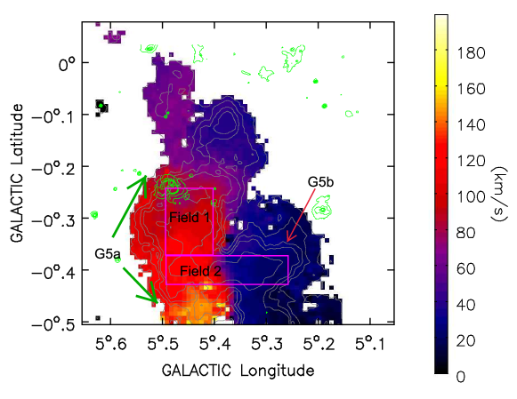
Figure 3: Velocity field (colours) and integrated intensity contours (grey) from the NH₃ (3,3) Mopra HOPS Survey (hops3; hops1; hops2). The contour levels of the grey moment 0 are [0.2, 0.4, 0.6, 0.8, 1.5]. Green contours are from 70 micron Hi-GAL, with contour levels of [0.1, 0.2, 0.4, 0.6, 0.8] (higal2016). The magenta boxes outline the fields. The clouds G5a and G5b are labeled.

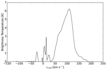
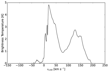
Figure 4: Averaged spectra of ^12CO $2\shortrightarrow 1$ over the two fields defined in Figure 3. Top: Field 1, which contains emission from cloud G5a from velocities to that continues down into Field 2 at a higher velocity, and also a line of sight HII region disassociated with G5 at a lower velocity. Bottom: Field 2, which contains emission from both clouds G5a and G5b. We identify G5a as associated with the emission from to , and G5b as the emission from to . G5b likely continues in emission to $\sim$ , but overlap with line of sight emission from ^12CO associated with the Galactic disk prevents it from being included.

The ALMA Atacama Compact Array (ACA) was used to observe the molecular clouds B1 and G5 (project code 2018.1.00862.S). Both 7m and Total Power observations were made. Only the Total Power observations of G5 are investigated in this paper. The Total Power array has a resolution of $\sim$ $30\text{\,}{}^{\prime\prime}$ in Band 6 (around 220 GHz), which was used to observe in the pertinent spectral lines. We show an overview of G5 as shown in NH3 (3,3) emission in the Mopra HOPS Survey (hops3; hops1; hops2). We observed G5 with two rectangular fields based on the intensity in NH3, one roughly along the middle of the north-south extent of the cloud and one along the east-west. The observed fields are boxed in magenta in Figure 3. The north-south extent we refer to as Field 1 (vertical in Fig 3) and the east-west (horizontal in Fig 3) as Field 2. The two fields overlap each other slightly. Figure 3 shows Field 1 consists of the vertical rectangular region extending over $0.375\text{\,}\mathrm{\SIUnitSymbolDegree}$ to $0.225\text{\,}\mathrm{\SIUnitSymbolDegree}$ in Galactic latitude and $5.4\text{\,}\mathrm{\SIUnitSymbolDegree}$ to $5.5\text{\,}\mathrm{\SIUnitSymbolDegree}$ in Galactic longitude. Field 2 in Figure 3 is a horizontal region extending over $-0.43\text{\,}\mathrm{\SIUnitSymbolDegree}$ to $-0.385\text{\,}\mathrm{\SIUnitSymbolDegree}$ in Galactic latitude and $5.48\text{\,}\mathrm{\SIUnitSymbolDegree}$ to $5.285\text{\,}\mathrm{\SIUnitSymbolDegree}$ in Galactic longitude. A total of $31\text{\,}\mathrm{h}\mathrm{o}\mathrm{u}\mathrm{r}\mathrm{s}$ on the Total Power array were used on the two fields.

Table 1: Correlator Configuration

Molecule and	Center Rest	Einstein	Collision Rates	Critical	Eff.	Velocity	Velocity
and	Frequency	A	($\mathrm{T\,=\,$60\text{\,}\mathrm{K}$}$)	Density	Ch.	Bandwidth	Resolution
Transition	$\mathrm{GHz}$	$\mathrm{s^{-1}\,\times 10^{-6}}$	$\mathrm{cm^{3}\,s^{-1}\,\times 10^{-11}}$	$\mathrm{cm^{-3}\,\times 10^{5}}$	#	$\mathrm{km\,s^{-1}}$	$\mathrm{km\,s^{-1}}$
^12CO $J=2\shortrightarrow 1$	230.53800000	0.691	6.0	0.115	3840	304.8	0.159
H(30)$\alpha$	231.9009278	-	-	-	3840	2424.2	1.263
H2CO $J=3_{2,1}\shortrightarrow 2_{2,0}$	218.760071	254.812	9.1	28.001	960	321.2	0.774
OCS $J=18\shortrightarrow 17$	218.9033565	30.371	7.4	4.104	-	-	-
HC3N v=0 $J=24\shortrightarrow 23$	218.32472	826.0	4.71	175.372	960	321.9	0.671
CH3OH $J=4_{2,2}\shortrightarrow 3_{1,2}$	218.440063	46.863	0.093	503.904	-	-	-
H2CO $J=3_{2,2}\shortrightarrow 2_{2,1}$	218.475642	253.822	9.1	27.893	-	-	-
H2CO $J=3_{0,3}\shortrightarrow 2_{0,2}$	218.222192	281.8	9.1	30.967	960	322.0	0.671
SiO v=0 $J=5\shortrightarrow 4$	217.104919	519.7	20.65	25.167	960	323.7	0.674
^13CO $J=2\shortrightarrow 1$	220.39868420	0.604	6.0	0.101	1920	318.8	0.332
C^18O $J=2\shortrightarrow 1$	219.56035410	0.601	6.0	0.1	1920	320.1	0.333

The correlator configuration includes several classes of astronomically important spectral lines simultaneously. The first are the isotopologues of carbon monoxide: ^12CO $J=2\shortrightarrow 1$, ^13CO $J=2\shortrightarrow 1$ and C^18O $J=2\shortrightarrow 1$. The second is SiO $J=5\shortrightarrow 4$, which is a strong shock tracer (schilke97) and should help determine how turbulent these clouds are as a result of shocks. Third is HC₃N $J=24\shortrightarrow 23$ as a dense gas tracer (mills2018). Fourth are the two formaldehyde lines, H2CO $J=3_{03}\shortrightarrow 2_{02}$ and H2CO $J=3_{22}\shortrightarrow 2_{21}$, which can be used together as a temperature tracer (mangum1993; ginsburg16). Fifth is the radio recombination line H(30)$\alpha$, which traces HII regions. This line is in a sub-band with the widest bandwidth to capture the potentially wide radio recombination line. The observation parameters of the spectral windows are included in Table 1. For the purposes of analysis, we ignore the spectral lines for OCS $J=18\shortrightarrow 17$, CH3OH $J=4_{22}\shortrightarrow 3_{12}$, and H2CO $J=3_{22}\shortrightarrow 2_{21}$.

3 Data Reduction

3.1 Target Description

G5 is a giant molecular cloud at $(\ell,b)=(+5.4,-0.4)$. The result of GravityCollab19 was that the distance to the Galactic Center is $8178\text{\,}\mathrm{p}\mathrm{c}$ with an error of 0.3%. The angle between the major axis of the Galactic bar and the Sun-GC line is less certain, but we will assume it to be $\sim$ $30\text{\,}\mathrm{\SIUnitSymbolDegree}$ $\pm$ $2\text{\,}\mathrm{\SIUnitSymbolDegree}$ (wegg2015; blandhawthorn2016). Assuming that G5 is located on the Galactic bar, and that the distance is uncertain by $\sim$ $1\text{\,}\mathrm{k}\mathrm{p}\mathrm{c}$ in the direction perpendicular to the bar major axis due to the finite width of the bar, we find using the Law of Sines that G5 is at a distance of $7.06\text{\,}\mathrm{k}\mathrm{p}\mathrm{c}$ $\pm$ $0.88\text{\,}\mathrm{k}\mathrm{p}\mathrm{c}$ from the Sun. The distance between G5 and the GC is $1.33\text{\,}\mathrm{k}\mathrm{p}\mathrm{c}$ $\pm$ $0.15\text{\,}\mathrm{k}\mathrm{p}\mathrm{c}$.

G5 has a projected extent of $48.9\text{\,}\mathrm{p}\mathrm{c}$ in Galactic latitude and $42.8\text{\,}\mathrm{p}\mathrm{c}$ long in Galactic longitude at a distance of $7\text{\,}\mathrm{k}\mathrm{p}\mathrm{c}$, using the approximate boundaries of the cloud seen in Figure 3 given by the Mopra HOPS NH3 (3,3) Survey (hops1; hops2; hops3). Two smaller clouds were found to make up G5 within our fields as shown in Figure 3. The first cloud, which we designate G5a, encompasses Field 1 and the east side of Field 2. The fields cover a projection of $\sim$ $22.0\text{\,}\mathrm{p}\mathrm{c}$ in Galactic latitude and $\sim$ $24.4\text{\,}\mathrm{p}\mathrm{c}$ in Galactic longitude. The second cloud we designate G5b, which takes up the west side of Field 2. Figure 4 shows the averaged spectra across the two fields.

We received 16 Total Power (TP) spectral cubes imaged using the ALMA pipeline calibration and imaging. We checked the cubes over for any flaws in the data cubes.

Next, we checked the rest frequencies of the spectral windows to ensure that they matched those that were targeted. We recorded the approximate velocities of notable spectral features.

3.2 Continuum Fitting

We found that Field 1 had poor baseline flatness. We used the CASA task imcontsub to fit a low-order polynomial to line-free channels, then subtracted the continuum model from the data.

For the CO isotopologues ^12CO and ^13CO, there were too few channels without lines to fit with a continuum model in Field 1. The poor baseline flatness caused dips in the spectrum in different spatial locations of the cubes, especially for ^12CO, causing the velocity integrated intensity in effected areas to be lowered. We masked out negative values, which are a result of baseline-oversubtraction, when creating moment maps (§4.1) and for line ratio measurements. This created an artifact in the ^12CO data at $(\ell,b)=(+5.413,-0.3725)$. We did not use Field 1 for any mass measurements, so the poor baselines in the field only affect our figures, not our measurements.

3.3 Baseline Ripple

We found that Field 2 shows a ripple in the spectral axis, which must be a residual of the baseline removal in the ALMA Single Dish pipeline. Single dish data often suffers from unstable baselines. Baseline ripples originate from multi-path reflections off of the structure of the telescope from a bright radio source, and can also occur in cables and other pieces of electronics. These reflections cause a standing wave in the optics, which makes a sine wave appear in each spectrum. The ALMA data reduction team had done baseline correction before imaging, however we found that Field 2 still showed residual ripples in the spectral cubes).

In an effort to remove the baseline ripple, the numpy.percentile function was used on the cubes to find the nth percentile of the data, with n varying between values of 1, 5 and 10 depending on the difference in strength between the ripple and the line. The nth percentile was determined by examining the output to ensure that no real data was being removed, while still removing the baseline ripple. Since the baseline ripple was constant spatially per cube, the nth percentile was then subtracted from each pixel. The percentile subtracted from each cube affected by baseline ripple is listed in Table LABEL:tbl:persub. The percentile subtraction method shifts the baseline away from zero, so a constant value was subtracted from each cube individually to return the baselines to zero. The vertical shift after percentile subtraction is listed in Appendix Table LABEL:tbl:persub for each cube affected by the baseline ripple. Removing the baseline ripple revealed dark structures on the resulting position velocity diagrams, constant spatially. The process of removing the baseline ripple is shown in Appendix Figure LABEL:fig:percentile.

3.4 Field Combination

We mosaicked the image data for the two fields to create one image. We combined the two fields by first finding a combined world coordinate system (WCS) and shape containing both fields using the reproject task find_optimal_celestial_wcs. Next, we created a new header of the resulting combined field by editing a copy of the existing header for one of the fields. We then used spectral_cube’s reproject function to regrid the cubes to the same WCS. We used the masks of the cubes to come up with a weighting grid, so that where the fields overlapped was valued at 2. We ran a loop over each channel of the cubes to combine them by adding each slice together and then dividing by the weighting grid to take the mean of the overlapping points. We then used the resulting array of values and the new header to create a combined cube containing both fields of G5.

3.5 Additional Molecular Line Detection

Additional molecular lines were detected in the selected spectral windows. These lines are listed in Table 1. For completeness, we identify these lines here.

In the H2CO $J=3_{21}\shortrightarrow 2_{20}$ spectral window, the additionally detected line is OCS $J=18\shortrightarrow 17$. The OCS line does not interfere with the H2CO line, but only a component of the line is included in the cube.

In the HC3N $J=24\shortrightarrow 23$ spectral window, there is no detection of HC3N. Instead, there are incomplete detections of a component of CH3OH $J=4_{22}\shortrightarrow 3_{12}$, p-H2CO $J=3_{22}\shortrightarrow 2_{21}$, and H2CO $3_{03}\shortrightarrow 2_{02}$. The HC3N cube spectrally overlaps the H2CO $3_{03}\shortrightarrow 2_{02}$ cube.

No further analysis was performed on the additional molecular lines.

4 Results

4.1 Moment Maps

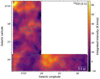
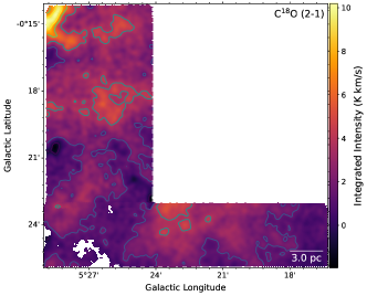
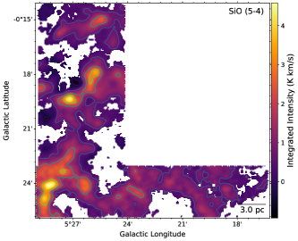
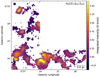
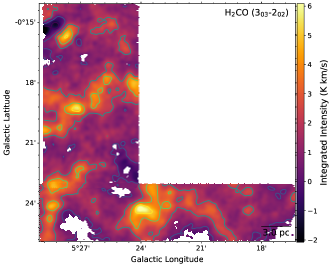
Figure 5: Integrated Intensity maps of the surveyed region of G5. First row: left image is ^12CO $J=2\shortrightarrow 1$, right image is ^13CO $J=2\shortrightarrow 1$. Second row: C^18O $J=2\shortrightarrow 1$, SiO $J=5\shortrightarrow 4$. Third row: H2CO $J=3_{22}\shortrightarrow 2_{21}$, H2CO $J=3_{03}\shortrightarrow 2_{02}$. The contours are the integrated intensity with five contours evenly spaced between the 0.25th and 99.75th percentiles.

Integrated intensity and velocity field maps were obtained for G5 using methods from the spectral-cube package for moment0 and moment1. We first spatially masked the cubes by considering only pixels where the peak was greater than 5 times the noise estimated from the median absolute deviation, then found the integrated intensity. We obtained the second moment and converted it to a FWHM using linewidth_fwhm from spectral-cube to make an intensity weighted velocity dispersion map, which computes a full-width at half maximum (FWHM) line width map across the spectral axis.

The moment 0, or integrated intensity, maps of all observed spectral lines are presented in Figure 5. The CO isotopologues all share a similar structure with a large feature in the middle of Field 1 stretching across it horizontally. There is also a feature at the bottom of Field 1 that extends into the Galactic east side of Field 2 across the averaged portion of the map smoothly. At the Galactic northeast corner of Field 1 is a very bright region of ^13CO $J=2\shortrightarrow 1$ and C^18O $J=2\shortrightarrow 1$ that shows up as a feature with absorption in ^12CO $J=2\shortrightarrow 1$. This part of the map overlaps with an HII region, as seen in Figure 3 with the 70 $\mu$m Hi-GAL (higal2016) contours. The HII region is not associated with G5a. The velocity of the HII region is with a FWHM of (wink83), which differs from that of G5a, which has velocities between and where the HII region overlaps.

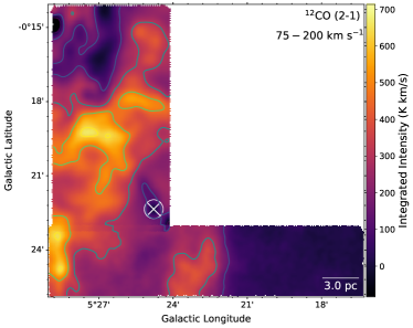
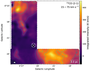
Figure 6: Two integrated intensity maps of G5 in ^12CO $J=2\shortrightarrow 1$ to show the distinct velocity components. Top: Integrated intensity map of G5a, from velocities to . Bottom: Integrated intensity map of G5b, from velocities to . This map was taken starting from to avoid emission from line of sight clouds in the Milky Way’s spiral arms.

Figure 6 shows integrated intensity maps separated into chunks from to for G5a and to for G5b. The top image of G5a shows a velocity component that runs down the length of Field 1 and down into Field 2. The bottom image of G5b also shows some of the CO emission likely associated with the overlapping HII region in Field 1.

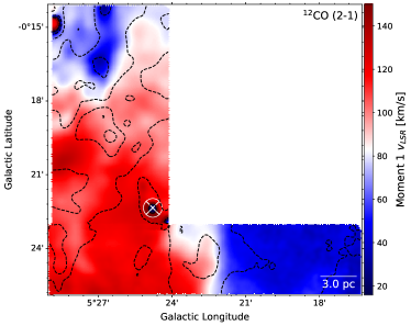
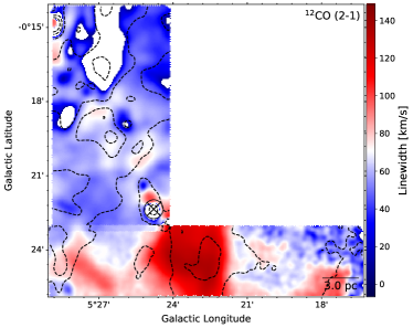
Figure 7: (Left) Velocity field map of ^12CO $J=2\shortrightarrow 1$. The red marks the high velocity cloud, and darker blue the low velocity cloud. The lighter blue in the Galactic northeast of the plot is gas associated with the overlapping HII region. Note that the HII region has a different velocity from the nearby G5 gas. (Right) Velocity dispersion map of ^12CO $J=2\shortrightarrow 1$. The elevated dispersion in red marks the interface between the two clouds where they overlap. Note that the elevated dispersion is due to overlapping spectral features, see Figure 9. There is not a very wide spectral feature over all of the area. Black dashed line contours are ^12CO $J=2\shortrightarrow 1$ integrated intensity with five contours evenly spaced between the 0.25th and 99.75th percentiles.

The left image in Figure 7 is a velocity field map of G5. The figure clearly shows that G5 contains two major velocity components. The red G5a in the Galactic east and the blue G5b in the Galactic west are separated by a white transition between the velocity components, which approximately lines up with a peak in ^12CO $J=2\shortrightarrow 1$ as shown by the contours.

The light blue region in the Galactic northeast of Figure 7 is gas associated with the HII region along the same line of sight as G5.

The right image in Figure 7 is a velocity dispersion map of G5. The blue shows the FWHM where the clouds are not overlapping or interacting. The red marks a heightened region of velocity dispersion due to the overlap and interaction between the two clouds. The apparently large velocity dispersion in the center of the image, caused by two separate velocity components, of up to $\sim$ should not be confused with internal dispersion of the gas in the clouds. The large velocity dispersion is reflecting the velocity gap between the two spatially overlapping detections of ^12CO $J=2\shortrightarrow 1$, not the FWHM of the molecular lines. The typical line widths in G5 are on the order of to .

4.2 Position-Velocity Diagram

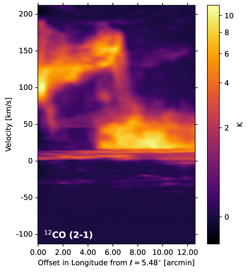
Figure 8: Position-Velocity diagram of Field 2 in ^12CO $J=2\shortrightarrow 1$, averaged over Galactic latitude and taken horizontally across the field with a width of $2\text{\,}\mathrm{\SIUnitSymbolArcminute}$. Features are labelled in Appendix Figure LABEL:fig:labelled_pv.

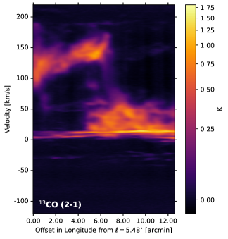
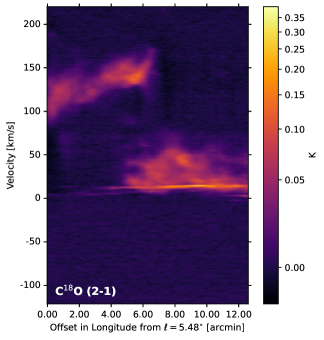
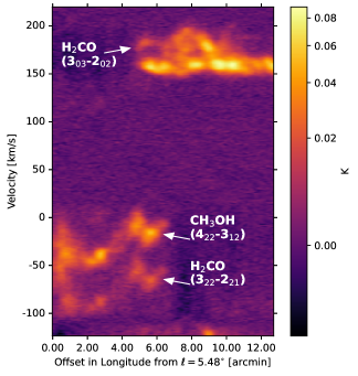
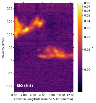
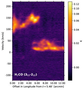
Figure 9: Position-Velocity Diagrams of Field 2 of G5, scaled by asinh. First row: first image is ^13CO $J=2\shortrightarrow 1$ second image is C^18O $J=2\shortrightarrow 1$. Second row: HC3N $J=24\shortrightarrow 23$, H2CO $J=3_{21}\shortrightarrow 2_{20}$. Third row: SiO $J=5\shortrightarrow 4$, H2CO $J=3_{03}\shortrightarrow 2_{02}$. The PV Diagram of HC3N has no detection of HC3N, but it is contaminated with emission from H2CO $J=3_{03}\shortrightarrow 2_{02}$ ($150\text{\,}\mathrm{km~{}s}^{-1}$ to $200\text{\,}\mathrm{km~{}s}^{-1}$), CH3OH $J=4_{22}\shortrightarrow 3_{12}$ ($-50\text{\,}\mathrm{km~{}s}^{-1}$ to $0\text{\,}\mathrm{km~{}s}^{-1}$) and H2CO $J=3_{22}\shortrightarrow 2_{21}$ ($-100\text{\,}\mathrm{km~{}s}^{-1}$ to $-50\text{\,}\mathrm{km~{}s}^{-1}$). The PV Diagram of H2CO H2CO $J=3_{21}\shortrightarrow 2_{20}$ is contaminated with emission from OCS $J=18\shortrightarrow 17$ at velocities between $-100\text{\,}\mathrm{km~{}s}^{-1}$ and $-50\text{\,}\mathrm{km~{}s}^{-1}$.

We created a position-velocity (PV) diagram, Figure 8, by selecting a range of data horizontally in Galactic Longitude across Field 2 for the ^12CO $2\shortrightarrow 1$ cube, with a width of $2\text{\,}\mathrm{\SIUnitSymbolArcminute}$. The offset of Figure 8 is relative to the left of Field 2 at $\ell=$$5.48\text{\,}\mathrm{\SIUnitSymbolDegree}$, so $0\text{\,}\mathrm{\SIUnitSymbolArcminute}$ is at a higher Galactic longitude. PV diagrams for the other observed spectral windows are shown in Figure 4.2.

We identify several features in the PV diagram in Figure 8. We first find G5a on the left side of the field at $\sim$, stretching from a position offset of $\sim$$0\text{\,}\mathrm{\SIUnitSymbolArcminute}$ to $\sim$$6\text{\,}\mathrm{\SIUnitSymbolArcminute}$. A second cloud with a wide velocity dispersion on the right side of the field is identified as G5b, which is at $\sim$ but stretches to $\sim$, from a $5\text{\,}\mathrm{\SIUnitSymbolArcminute}$ to $12\text{\,}\mathrm{\SIUnitSymbolArcminute}$ offset. Stretching between the two clouds in the velocity domain at an offset of $\sim$ $7\text{\,}\mathrm{\SIUnitSymbolArcminute}$ is a velocity bridge.

A velocity bridge is a feature in a PV diagram which is wide in velocity space but relatively narrow in position space, and connects the two features at $\sim$ and at $\sim$, spatially the velocity bridge is where the two clouds overlap (HaworthDec15; HaworthJun15). The ^12CO PV diagram in Figure 8 has a vertical velocity bridge connecting the two clouds. We discuss the details and implications of the velocity bridge feature in Section LABEL:sec:velocitybridge.

The clump at offset $5\text{\,}\mathrm{\SIUnitSymbolArcminute}$ and at the velocity could be associated with a secondary bar lane feature identified in sormani19 and Liszt2006, or it is somehow associated with the velocity bridge.

We find another extended velocity feature of similar spectral width to the velocity bridge on the left side of the field at approximately $(\ell,b)=(5.47,-0.41)$$\text{\,}\mathrm{\SIUnitSymbolDegree}$, which seems connected to G5a, but does not seem to directly link it to the G5b. The feature has an unusually wide velocity from $\sim$ to $\sim$ where it intersects with G5a at around a $0.5\text{\,}\mathrm{\SIUnitSymbolArcminute}$ offset. While this feature does not seem to directly intersect with G5b, there is a cloud feature at $\sim$