EMPIRICALLY DRIVEN SPLINE BASES FOR FUNCTIONAL PRINCIPAL COMPONENT ANALYSIS IN 2D

Abstract

Functional data analysis is typically performed in two steps: first, functionally representing discrete observations, and then applying functional methods to the so-represented data. The initial choice of a functional representation may have a significant impact on the second phase of the analysis, as shown in recent research, where data-driven spline bases outperformed the predefined rigid choice of functional representation. The method chooses an initial functional basis by an efficient placement of the knots using a simple machine-learning algorithm. The approach does not apply directly when the data are defined on domains of a higher dimension than one such as, for example, images. The reason is that in higher dimensions the convenient and numerically efficient spline bases are obtained as tensor bases from 1D spline bases that require knots that are located on a lattice. This does not allow for a flexible knot placement that was fundamental for the 1D approach. The goal of this research is to propose two modified approaches that circumvent the problem by coding the irregular knot selection into their densities and utilizing these densities through the topology of the spaces of splines. This allows for regular grids for the knots and thus facilitates using the spline tensor bases. It is tested on 1D data showing that its performance is comparable to or better than the previous methods.

1 Introduction

The data-driven knot selection algorithm (DDK), see [1], identifies regions in the common domain of functional data that feature high curvatures and other significant systematic variability. By strategically placing knots in these regions, the algorithm effectively captures the systematic variation and is available as a package on the GitHub repository [2]. In the one-dimensional domain case, the placement of knots can be directly utilized in the choice of the splines spanned over selected knots and it has been proved that this improves the efficiency of the functional representation of the data and the ensuing statistical analysis. The reason behind the improvement is dimension reduction in the initial representation of the data achieved by a ‘clever’ choice of the knots. Figure 1 (top) presents the knot selection for the wine spectra (left) and their derivatives (right), see [3]. Once the knots are provided, one can build the splinet i.e. a convenient orthonormal spline basis spanned over these knots, [4]. How the choice of the knots can improve the analysis of the data is shown in Figure 1 (bottom), where we see the projection of the data to the first four principal components for equally spaced knots (left) and for the optimized data-driven knot selection (right).

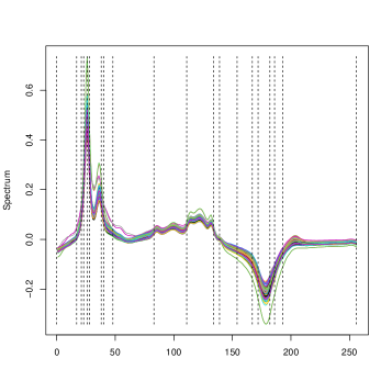
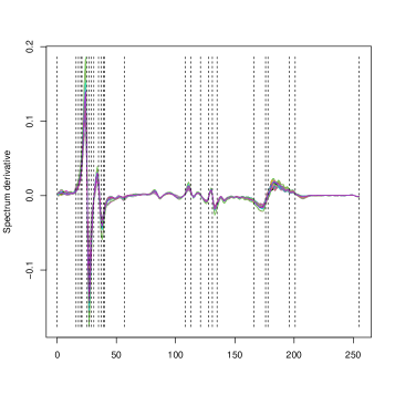
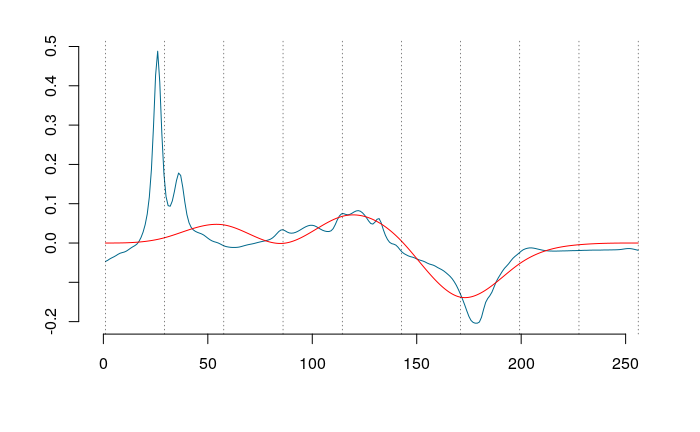
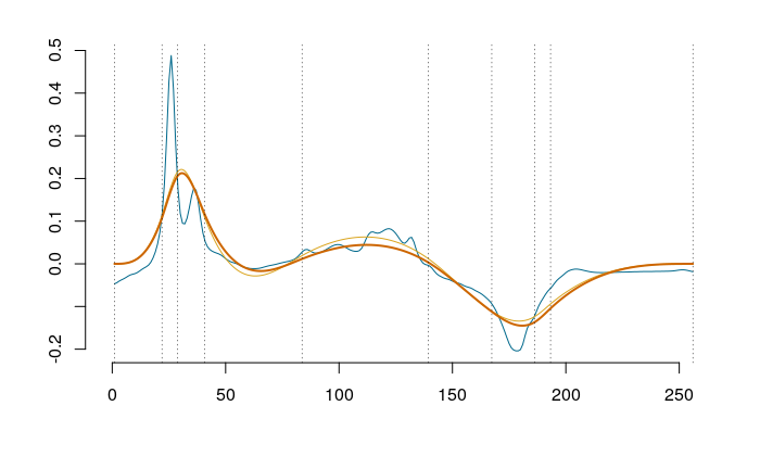
Figure 1: 1D data and the knot selection. (Top): 1D case, the wine data, the knots are marked by vertical dashed lines. (Bottom): Projection to the first four principal component for equally spaced (left) and data-driven, optimally spaced knots (right).

In 2D, one can utilize tensor product spline bases only, since the knots reside on the regular lattice knots. On the other hand, if one chooses ‘knots’ to optimize the mean square error (MSE), the selected ‘knots’ are irregular and they cannot be used directly to build convenient spline bases. In this note, we discuss how an irregular ‘knot’ selection can be utilized to modify the approach that allows the use of the tensor bases but at the same time accounts for the data-driven ‘knot’ selection. In fact, the bases will be constructed on equally spaced knots which have an additional computational advantage. The approach is through utilizing the obtained irregular ‘knot’ distribution to change the topology of spline spaces. The two methods of doing this will be considered: the first one is based on changing the topology of the state space (the space of values of splines) and the second one is based on transforming the domain space of splines.

The note is organized as follows. In the next section, we briefly recap basic facts about the orthonormal basis of spline called splinets, which were recently introduced in [5]. There, we also define two dimensional orthonormal tensor splinets. This is followed by a section on the proposed method of the knot selection in 2D. The two methods considered in this note are described in the two subsequent sections. First, the state-space transformation method is discussed in the 1D case and then explain the analogous approach to the 2D case. A similar scheme is followed in the section on the domain transformation method. A description of empirical studies that are designed to test the methods is concluded in the note.

2 Tensor splinets

The splinets are efficient orthonormal bases of splines discussed in full detail in [5] and implemented in the $R$-package Splinets, [6]. For the purpose of this note, it is enough to know that a splinet is obtained by an efficient dyadic algorithm from $B$-splines spanned on a given set of knots. Two examples are shown in Figure 2, where the effect of different knot distributions is clearly seen.

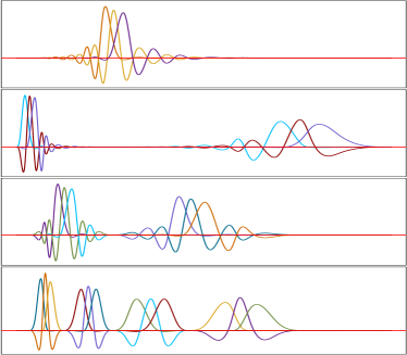
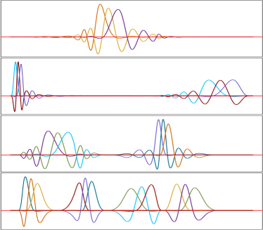
Figure 2: Examples of splinets of the third order in the graphical representation of the dyadic pyramid. In the figure, we see that placement of knots changes the ability to model local variability in the data.

In the package, the focus is on one-dimensional domains. However, the tensor product bases are simple enough that the package can also be utilized for the analysis of functional data defined in a two-dimensional space.

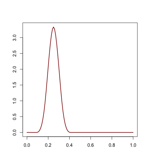
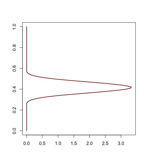
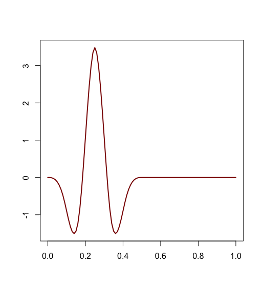
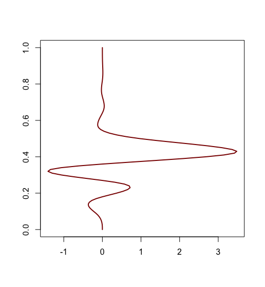
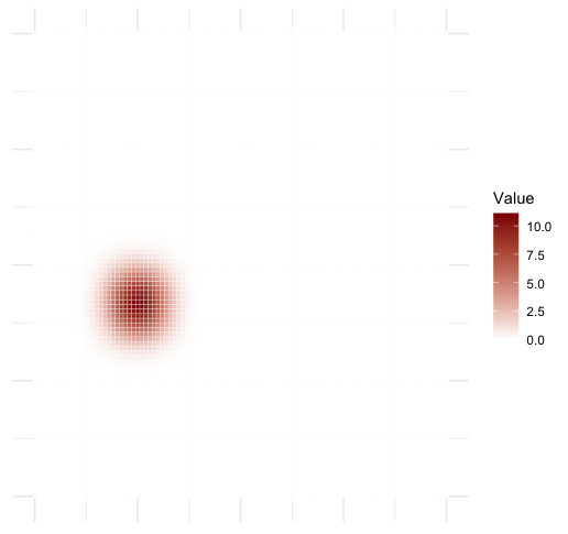
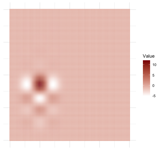
Figure 3: Top: Two $B$-splines (left) and corresponding $OB$-splines (right). Bottom: The corresponding tensor spline $B_{\boldsymbol{\xi}i}^{k}\otimes B_{\boldsymbol{\xi},i}^{l}$ (left) and the orthogonal tensor spline $OB_{\boldsymbol{\xi}i}^{k}\otimes OB_{\boldsymbol{\xi},i}^{l}$(right).

Let us consider two knot selections $a=\xi_{0}<\dots<\xi_{n+1}=b$ and $c=\zeta_{0}<\dots<\zeta_{m+1}=d$ on interval $[a,b]$ and $[c,d]$, respectively. Further, let us consider two sets of $B$-splines $\{B_{\boldsymbol{\xi}i}^{k}(x)\}$, $i=1,\dots,n-k+1$, $x\in[a,b]$ and $\{B_{\boldsymbol{\zeta}j}^{l}(y)\}$, $j=1,\dots,m-l+1$, $y\in[c,d]$ of orders $k$ and $l$, respectively, and spanned over the respective set of knots. The linear functional spaces spanned on these sets of $B$-splines are denoted by $\mathcal{H}^{k}_{\boldsymbol{\xi}}$ and $\mathcal{H}^{l}_{\boldsymbol{\zeta}}$, respectively. Then the tensor product $B$-spline basis is defined as

$$\left(B_{\boldsymbol{\xi}i}^{k}\otimes B_{\boldsymbol{\zeta}j}^{l}\right)(x,y)=B_{\boldsymbol{\xi}i}^{k}(x)B_{\boldsymbol{\zeta}j}^{l}(y),\,(x,y)\in[a,b]\times[c,d].$$ (1)

Let $\mathcal{H}^{k}_{\boldsymbol{\xi}}\otimes\mathcal{H}^{l}_{\boldsymbol{\zeta}}$ be the $(n-k+1)(m-l+1)$-dimensional linear functional space on $[a,b]\times[c,d]$ spanned by the tensor product basis.

Theorem 2.1.

Let $f$ be square-integrable function on $[a,b]\times[c,d]$ and the splinets $\{OB_{\boldsymbol{\xi}i}^{k}\}_{i=1}^{n-k+1}$ and $\{OB_{\boldsymbol{\xi},i}^{l}\}_{j=1}^{m-l+1}$ are the orthogonormal splines bases obtained by dyadic orthogonalization of $B_{\boldsymbol{\xi}i}^{k}$ and $B_{\boldsymbol{\xi}j}^{l}$, respectively. Then

$$\left\{OB_{\boldsymbol{\xi}i}^{k}\otimes OB_{\boldsymbol{\zeta}j}^{l}\right\}_{i,j=1}^{n-k+1,m-l+1}$$

also constitute an orthonormal basis in $\mathcal{H}^{k}_{\boldsymbol{\xi}}\otimes\mathcal{H}^{l}_{\boldsymbol{\zeta}}$ and the projection $\hat{f}$ of $f$ to this space is given by

$$\hat{f}=\sum_{i=1}^{n-k+1}\sum_{j=1}^{m-l+1}\alpha_{ij}\cdot OB_{\boldsymbol{\xi}i}^{k}\otimes OB_{\boldsymbol{\zeta}j}^{l},$$

where $\alpha_{ij}=\int_{a}^{b}OB_{\boldsymbol{\xi}i}^{k}(x)\int_{c}^{d}OB_{\boldsymbol{\zeta}j}^{l}(y)f(x,y)~{}dy~{}dx$.

Moreover, for each $f$ satisfying zero boundary conditions of the order $l$ and $m$ along $[a,b]\times\{0\}$ and $\{0\}\times[c,d]$, respectively, any $k$ and $l$, each $\epsilon>0$ there exist knot selections $a=\xi_{0}<\dots<\xi_{n+1}=b$ and $c=\zeta_{0}<\dots<\zeta_{m+1}=d$ such that

$$\left(\int_{a}^{b}\int_{c}^{d}\left|f(x,y)-\hat{f}(x,y)\right|^{2}~{}dx~{}dy\right)^{1/2}\leq\epsilon.$$

In Figure 3, we present abscissa and ordinate 1D-basis elements at the top and $B_{\boldsymbol{\xi}i}^{k}\otimes B_{\boldsymbol{\zeta}j}^{l}$ (left) and $OB_{\boldsymbol{\xi}i}^{k}\otimes OB_{\boldsymbol{\zeta}j}^{l}$ (right) at the bottom.

3 ‘Knot’ selection in 2D

The algorithm that has been used for the 1D knot selection is applicable to functional data that are defined on the 2D plane. Indeed, the method is equivalent to building a regression binary tree where the so-called split points (the nods at the tree) are found based on the best mean square error (MSE) approximation of a regression function by functions that are constant over a 2D grid, see [7]. The centers of rectangles of the 2D grid define ‘knots’ as shown in Figure 4 (left). The ‘knots’ for the MNIST fashion images and their gradient images are presented in Figure 4 (middle, right), see [8] for more details on this data set.

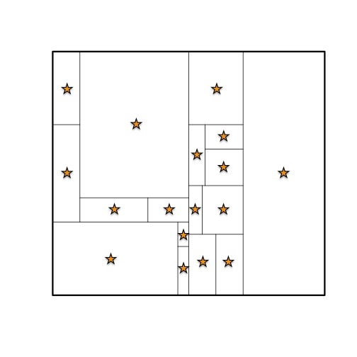
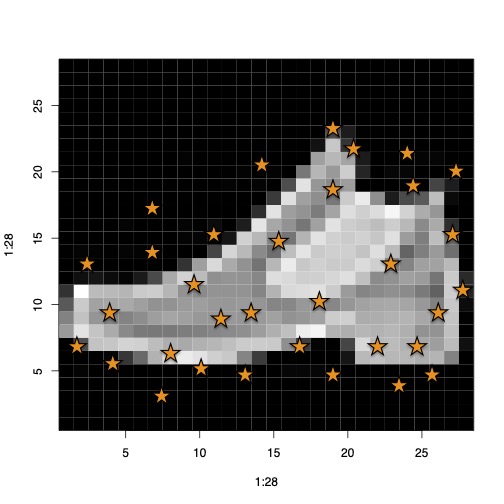
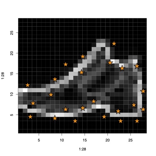
Figure 4: (Left): Illustration of how the ‘knots’ in 2D are obtained by taking the midpoints of 2D rectangular grid cells obtained by the binary regression tree MSE fit to the functional data. (Middle) The original image and the selected ‘knots’, (Right) The gradient image with ‘knots’.

We are using quotation marks when referring to obtained points since they are not convenient to build direct spline approximation in a similar manner as in the one-dimensional case. The reason for this is that there are no convenient spline bases spanned on irregularly distributed ‘knots’ in such domains. One could consider triangulation but defining splines on a triangular grid is complicated and the resulting spline bases are difficult to orthogonalize. The easiest to use and most popular 2D space of splines are based on the tensor product bases, see, for example, [9]. However, the tensor bases are defined over lattice grids, and thus the 2D grids shown in Figure 4 (Bottom) cannot be directly used for constructing such bases.

4 The state space transformation

The problem of irregularly spread ‘knots’ occurs only for domains of a dimension higher than one. Our proposed methods account for ‘knots’ distribution not directly in the construction of spline bases and can be applied in 1D as well. In this case, the irregular knots can be used directly in building splines thus one can benchmark the proposed methods against this direct irregular knot selection.

The main component of both methods is a continuous approximation of the irregular ‘knot’ distribution. We consider ‘knots’ $\boldsymbol{\xi}_{j}$, $j=1,\dots,N$ that are irregularly distributed. One can simply apply kernel-driven estimation-like methods known in non-parametric statistics by treating the ‘knots’ as iid data drawn from a certain distribution. Since ‘knots’ are not truly iid data, those methods should be viewed as ad hoc smoothing methods. More suitably, one can use Splinet-package to project discretized data to the space of splines as presented in Theorem 2.1. From now on, $g$ represents the density of the ‘knot’ distribution.

Small values of $g$ indicate regions where the data are less informational. This motivates us to introduce a $g$-weighted topology in $L^{2}_{g}=\{h:\int h^{2}g<\infty\}$

$$\langle h,h\rangle_{g}=\int h^{2}(x)g(x)dx=\int\left(h(x)\sqrt{g(x)}\right)^{2}dx=\langle h\sqrt{g},h\sqrt{g}\rangle,\ \ \ \forall h\in L^{2}_{g}.$$

We can transfer the functional data $X_{1},X_{2},\dots,X_{n}$ to

$$\tilde{X_{i}}(x)=X_{i}(x)\sqrt{g(x)}.$$ (2)

One can use $\tilde{X_{1}}(x),\tilde{X_{2}}(x),\dots,\tilde{X_{n}}(x)$ instead of the original data and perform any functional analysis with one important modification. Namely, since the knot distribution is already accounted for, one does not need to use splines built on irregularly distributed knots. This is crucial in the 2D case since the equally spaced knots constitute a lattice on which tensor splines are well defined.

Remark 4.1.

The sparsity of ‘knots’ in some regions may lead to zero (or nearly zero) values of $g$. This may lead to a subdomain of the original $[a,b]\times[c,d]$. This subdomain could constitute the support of the functional data. To benefit from that one would like to have the possibility to account for a reduced support set. This feature is actually implemented in the current version of Splinets-package but will be extended to the two-dimensional case in order to utilize sparsity of the images.

5 The domain space transformation

Here, we also consider the ‘knots’ distribution but instead of the density $g$, we utilize the distribution function $G(x,y)=\int_{a}^{x}\int_{c}^{y}g(u,v)~{}du~{}dv$. For that $g$ approximated in the previous method can be used. Alternatively, one can direct approach to the problem by looking at the ‘empirical’ equivalent

$$\hat{G}(x,y)=\frac{\#\{{\boldsymbol{\xi}}\cap[a,x]\times[c,y]\}}{N}.$$

Then $\hat{G}$ can be used to construct domain mapping $\mathbf{G}$ from $[a,b]\times[c,d]$ to $[0,1]\times[0,1]$ such that $\mathbf{G}(\boldsymbol{\xi})$ are uniformly distributed.

To simplify the discussion in this note we consider only the one-dimensional case. Let $\nu_{i}={G}_{X}(\xi_{i})$, yielding approximately uniformly distributed $\nu_{1},\ldots,\nu_{n}$. Thus our functional data point, say $h$, needs to be transformed to $\tilde{h}=h\circ G^{-1}$. For these domain-transformed data, we have

$$\langle\tilde{h},\tilde{k}\rangle =\int_{0}^{1}h(G^{-1}(u))k(G^{-1}(u))~{}du=\int_{0}^{1}h(x)k(x){g(x)}~{}du=\langle h,k\rangle_{g}$$

We conclude that while the two methods transform data in different ways they are topologically equivalent.

Theorem 5.1.

Let $g$ be the density distribution on $[0,1]$, $G$ be the corresponding cdf. Moreover, let $h_{g}=\sqrt{g}h$ for $h\in L_{g}^{2}$ and $\tilde{h}_{G}=h\circ G^{-1}$, then

$$\langle h_{g},k_{g}\rangle=\langle\tilde{h}_{G},\tilde{k}_{G}\rangle.$$

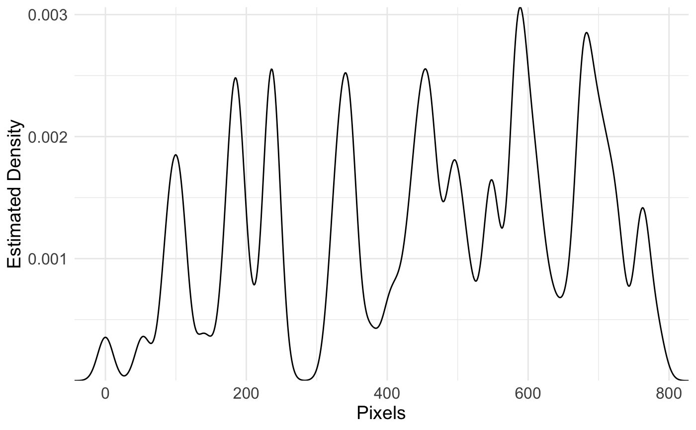
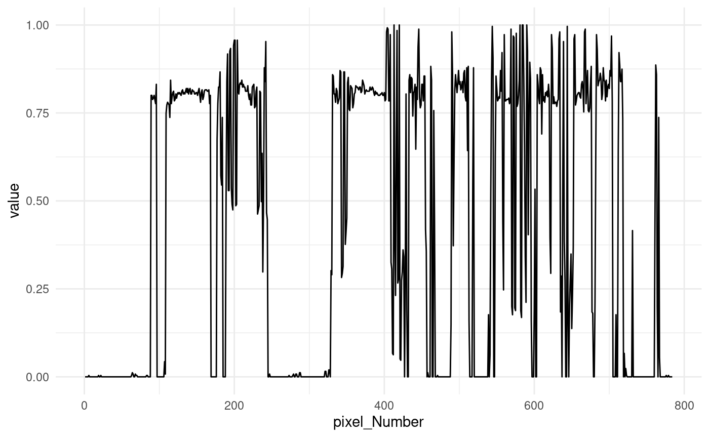
Figure 5: Left: Approximated density of knots for the data-driven approach. The knots were selected using the DDK package. Right: One-dimensional Hilbert curve representations of one sample from the T-shirt class from the MNIST data.

6 Data analysis

To assess the efficiency we utilize the fashion MNIST image dataset. For simplicity, we focus on one class of this dataset, the T-shirt class. The performance was compared with the conventional equidistant and the full data-driven knot selection methodologies detailed in [1]. Since we focus in this note on the 1D analysis (leaving a fully 2D discussion for a full paper), we looked at the images only as one-dimensional vectors. However, to better account for spatial dependencies in the images, we used the Hilbert curve to order the pixels in this vector, for more details see [10].

Our experiment was organized into three distinct workflows. In the first workflow (W1), we employ the traditional strategy of equidistant knot selection. Subsequently, in the second workflow (W2), we leveraged the Data-Driven Knot (DDK) selection algorithm detailed in the aforementioned citation to select the knots. Finally, in the third workflow (W3), which encapsulates our proposed methodology, we utilized the knots selected from the DDK algorithm to generate the corresponding density function using the KernSmooth R package. The image data was then weighted by this density function, following the process outlined in (2).

In all three workflows, following the selection of the knots, we employ the Splinets R package to project the data onto third-order splines with the selected knots. Subsequently, we perform a spectral decomposition of the data by estimating the eigenvalues, denoted $\lambda_{i}$, and the corresponding eigenfunctions. Next, we compute the explained variance for each of the three workflows, labeled $EV_{1}$, $EV_{2}$, and $EV_{3}$. To achieve this, we first perform PCA on our original data set to obtain a set of eigenvalues $\Lambda_{k}$, $k=1,\ldots,784$.

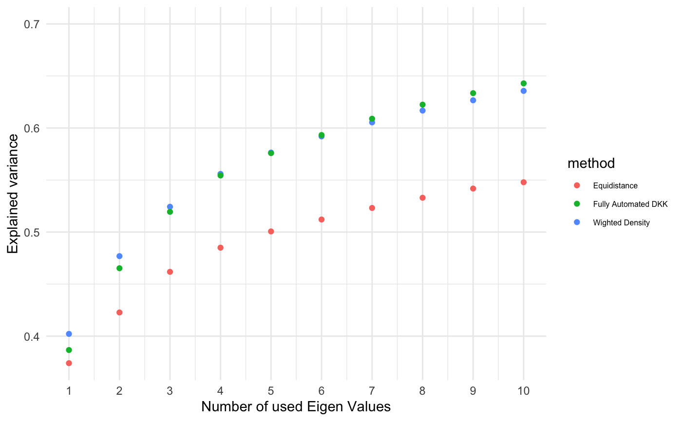
Figure 6: Explaind variance for the three workflows

For each workflow, we obtained a set of eigenvalues, which are derived from the projection of the data to the corresponding workflow subspace. That is for $i=1,2,3$ we get $\lambda_{j}^{(i)}$, $j=1,\ldots,n$, where $n$ is a pre-specified number of eigenvalues that we want the explained variance with respect to. The explained variance $EV_{i}$ for each workflow $i$ is then calculated using

$$EV_{i}=\frac{\sum_{j=1}^{n}\lambda_{j}^{(i)}}{\sum_{k=1}^{784}\Lambda_{k}.}$$

This equation quantifies the proportion of the total variance in the original data that is captured by $n$ eigenvalues in the subspace resulting from each workflow. In Figure 6, we observe the $W2$ and $W3$ provide better-explained variance compared to $W1$. For example, for $n=10$ we have $EV_{1}=0.547,EV_{2}=0.635,EV_{3}=0.642$.

References

- [1] Basna, R., Nassar, H., Podgórski, K.: Data driven orthogonal basis selection for functional data analysis. Journal of Multivariate Analysis 189, 104,868 (2022)
- [2] Basna, R., Nassar, H., Podgórski, K.: R-Package: DKK, Version: 0.1.0, Orthonormal Basis Selection using Machine Learning (2021). URL https://github.com/ranibasna/ddk
- [3] Meurens, M.: Wine – data set. Online. URL https://rdrr.io/cran/cggd/man/Wine.html
- [4] Podgórski, K.: Splinets – splines through the taylor expansion, their support sets and orthogonal bases (2021)
- [5] Liu, X., Nassar, H., Podgórski, K.: Dyadic diagonalization of positive definite band matrices and efficient b-spline orthogonalization. Journal of Computational and Applied Mathematics 414, 114,444 (2022). https://doi.org/10.1016/j.cam.2022.114444. URL https://www.sciencedirect.com/science/article/pii/S0377042722002102
- [6] Liu, X., Nassar, H., Podgórski, K.: Splinets: Functional Data Analysis using Splines and Orthogonal Spline Bases. CRAN.R-project.org (2023). R package version 1.5.0
- [7] Hastie, T., Tibshirani, R., Friedman, J.: The elements of statistical learning: data mining, inference and prediction, 2 edn. Springer (2009). URL http://www-stat.stanford.edu/~tibs/ElemStatLearn/
- [8] Fashion MNIST - data set. Online, Zalando Research. URL https://www.kaggle.com/datasets/zalando-research/fashionmnist?resource=download
- [9] Eilers, P., Marx, B.: Practical smoothing. The joys of -splines. Cambridge University Press, Cambridge (2021)
- [10] Bader, M.: Space-filling curves: an introduction with applications in scientific computing, vol. 9. Springer Science & Business Media (2012)