Biomedical Image Splicing Detection using Uncertainty-Guided Refinement

Abstract

Recently, a surge in biomedical academic publications suspected of image manipulation has led to numerous retractions, turning biomedical image forensics into a research hotspot. While manipulation detectors are concerning, the specific detection of splicing traces in biomedical images remains underexplored. The disruptive factors within biomedical images, such as artifacts, abnormal patterns, and noises, show misleading features like the splicing traces, greatly increasing the challenge for this task. Moreover, the scarcity of high-quality spliced biomedical images also limits potential advancements in this field. In this work, we propose an Uncertainty-guided Refinement Network (URN) to mitigate the effects of these disruptive factors. Our URN can explicitly suppress the propagation of unreliable information flow caused by disruptive factors among regions, thereby obtaining robust features. Moreover, URN enables a concentration on the refinement of uncertainly predicted regions during the decoding phase. Besides, we construct a dataset for Biomedical image Splicing (BioSp) detection, which consists of 1,290 spliced images. Compared with existing datasets, BioSp comprises the largest number of spliced images and the most diverse sources. Comprehensive experiments on three benchmark datasets demonstrate the superiority of the proposed method. Meanwhile, we verify the generalizability of URN when against cross-dataset domain shifts and its robustness to resist post-processing approaches. Our BioSp dataset will be released upon acceptance.

1 Introduction

Biomedical images, as essential components of biomedical academic publications, always serve to demonstrate experimental results (Miura and Nørrelykke 2021). As shown in Fig. 1(a), malicious researchers can manipulate the images to fabricate experimental conclusions or conceal unfavorable results (Bucci 2018), which pose significant threats to the scholarly community (Rossner and Yamada 2004).

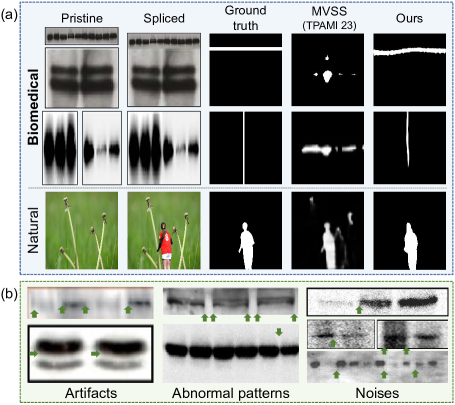
Figure 1: (a) Difference between spliced biomedical (top two rows) and natural image (bottom one row). Examples of splicing detection results on the two kinds of images predicted by our method and a SoTA natural image manipulation detection method, i.e. MVSS (Dong et al. 2023). (b) Disruptive factors such as artifacts, abnormal patterns, and noises in biomedical images. The green arrows indicate regions interfered with disruptive factors where the SoTA manipulation detectors designed for natural images are prone to give false alarms.

With advancements in deep learning and the availability of biomedical image forensics datasets (Sabir et al. 2021; Cardenuto and Rocha 2022; Koker et al. 2020), notable progresses have been made in detecting duplications (Koker et al. 2020; Moreira et al. 2022; Sabir et al. 2022) and copy-move manipulations (Moreira et al. 2022).

However, splicing, as one of the most commonly used manipulations for biomedical images, is more challenging to detect but receives less attention. To the best of our knowledge, no method has been specifically proposed for biomedical image splicing detection. It seems to be a feasible way to train models designed for natural images on biomedical datasets. Yet, existing natural image manipulation detectors, whether proposed for splicing detection (Bi et al. 2019) or general purposes (Guillaro et al. 2023; Kwon et al. 2022; Guo et al. 2023), cannot achieve satisfactory performance on biomedical datasets (Sabir et al. 2021). We attribute the failure to two primary reasons: (1) the prevalence of more disruptive factors in biomedical images and (2) the limited number of spliced images for training. Such disruptive factors can mislead detection methods, resulting in false alarms and incomplete predictions. These factors, illustrated in Fig. 1(b), are enumerated as follows. (1) Artifacts. Biomedical images always undergo multiple types of non-malicious degradation by authors and publishers. Commonly used degradations, e.g. JPEG compression, can decrease tampering traces and bring more artifacts (Wu et al. 2022). (2) Abnormal patterns. During experimental processes, operational mistakes (e.g., improper reagent ratios and gel rupture) can result in abnormal patterns, which tend to be confused with spicing traces. (3) Noises. Malfunctions and degradations of imaging devices or even simple operator errors can introduce a large amount of noises.

Furthermore, individuals with malicious intent can use advanced image editing tools such as Photoshop (Zhuang et al. 2021) or SoTA generative models, e.g., Generative Adversarial Networks (GAN) (Suvorov et al. 2022) and diffusion models (Rombach et al. 2022), to post-process the spliced images. These post-processing approaches is able to reduce visible clues of tampering, making it difficult to distinguish between the natural boundaries and splicing traces.

To address such issues, we aim to design a resilient framework that can resist disruptive factors and unknown post-processing approaches. As shown in Fig. 2, we propose a two-stage Uncertainty-guided Refinement Network (URN). In stage one, our URN recognizes uncertainly predicted regions affected by disruptive factors using Monte Carlo Dropout (MCD). In the second stage, it integrates uncertainty to perform refinement. To fully exploit uncertainty information, we proposed Uncertainty-Guided Graph Convolution (UGGC) modules. The UGGC limits the unreliable information flow from uncertain regions but guides them to receive information from nearby confident regions. This ensures that the uncertain nodes can be gradually refined with less interference. In addition, we propose Uncertainty-Enhanced Manipulation Attention (UEMA) modules, which can focus on ambiguously predicted regions with high uncertainty and help distinguish spliced and pristine areas. By combining UGGC and UEMA, the performance and robustness of our URN can be further improved.

Besides the effective methodologies, high-quality datasets are equally important for this task. Existing publicly available datasets (Sabir et al. 2021; Cardenuto and Rocha 2022) have a limited number of spliced images and lack source diversity. Therefore, we propose a dataset for Biomedical Splicing detection (BioSp), a diverse and challenging dataset surpassing others in size, source diversity, and splicing complexity. BioSp consists of two subsets: one is collected from public comments on the authoritative post-publication peer review platform PubPeer , while the other one comprises images manually manipulated with Photoshop.

Overall, our contributions include:

• We are the first to propose an end-to-end deep learning-based framework for biomedical image splicing detection. Our Uncertainty-guided Refinement Network (URN) can resist disruptive factors in biomedical images by fully using uncertainties to refine coarse predictions.

• We propose two modules, i.e., the Uncertainty-Guided Graph Convolution (UGGC) and Uncertainty-Enhanced Manipulation Attention (UEMA) to help URN integrate uncertainty information. UGGC is able to extract robust features against disruptive factors during encoding, while UEMA focuses on the refinement of uncertainly predicted areas in the decoding phase.

• We introduce a new dataset for Biomedical image Splicing (BioSp) detection. Compared with existing datasets, BioSp has the largest number of spliced images from diverse sources and various splicing approaches.

• We conduct comprehensive experiments on four benchmarks, demonstrating the efficacy of the proposed method in both pixel-level and image-level detection.

2 Related Works

2.1 Natural Image Manipulation Detection

The detection of manipulated pixels in natural images captured by digital cameras has been extensively studied, and several standard datasets are proposed for this purpose (Verdoliva 2020). In the early years, with the boost of deep learning techniques, GSR (Zhou et al. 2020), and RRU (Bi et al. 2019) successfully introduce end-to-end Convolutional Neural Networks (CNNs) for natural image manipulation detection. The effectiveness of self-attention mechanisms in this task has also been discussed by SPAN (Hu et al. 2020), TransForensics (Hao et al. 2021), and PSCC-Net (Liu et al. 2022). Analyzing intrinsic statistics to explore traces of image forgeries also gains progress (Kwon et al. 2021, 2022; Wang et al. 2022; Bi et al. 2023). Towards more generalized detection, many methods employ noise-sensitive filters (Zhou et al. 2018; Wu, AbdAlmageed, and Natarajan 2019; Dong et al. 2023; Lin et al. 2023) or self-supervised learning (Cozzolino and Verdoliva 2020; Guillaro et al. 2023) to suppress semantic information and analyze noise inconsistency of images. More recently, Hifi-Net (Guo et al. 2023) and HAMMER (Shao, Wu, and Liu 2023) expand this task, proposing fine-grained image forgery detection and multi-modal media forensics, respectively. Despite significant progresses, these SoTA methods cannot work well in biomedical images as the disruptive factors easily mislead them to make false alarms and incomplete predictions. It is still a challenge to obtain robust feature representations for biomedical images.

2.2 Uncertainty Estimation

Uncertainty can accurately reflect confidence of the prediction results of deep learning-based methods and has been widely applied in computer vision tasks such as semantic segmentation (Zheng et al. 2021). The success of uncertainty learning in other fields has also promoted its application for image forensics tasks, i.e., JPEG artifacts (Lorch, Maier, and Riess 2020), resample artifacts (Maier, Lorch, and Riess 2020), and evaluating the confidence of natural image forgery detection results (Guillaro et al. 2023).

Motivated by their works, we introduce uncertainty estimation for robust splicing feature representation learning. Unlike the aforementioned uncertainty-integrated methods, we make full use of uncertainty to recognize and refine uncertain predicted parts affected by disruptive factors.

2.3 Biomedical Image Forensics Datasets

Recent works, i.e., RSIID (Cardenuto and Rocha 2022), BINDER (Koker et al. 2020), and SYB (Mandelli et al. 2022), automate the forgery of biomedical images to generate large-scale forensics datasets, which are designed for the detection of manipulation, duplication, and synthesis, respectively. To prevent the negative effects brought by the domain gap between automatically generated images and real-world ones, Biofors (Sabir et al. 2021) extracts 47,805 biomedical images from papers published in PLOS ONE 2013, including 1,741 manipulated images with pixel-level labels according to raw annotations provided by biomedical experts (Bik, Casadevall, and Fang 2016).

Sufficient datasets are available for the detection of biomedical image duplication and copy-move manipulation. Significant progress has been made in these two tasks (Sabir et al. 2022; Moreira et al. 2022). However, the lack of high-quality datasets for biomedical splicing detection hinders the progress for this field. It can be seen in Tab. 1, the quantity of spliced images remains insufficient, especially in Biofors which only contains 181 blot/gel images. The lack of diversity in splicing approaches and image sources also hampers the training of a model with inspiring performance.

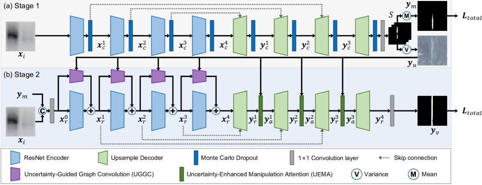
Figure 2: Overall structure of the proposed URN. It consists of two stages: (a) the stage-1 network makes coarse predictions of spliced regions and estimates the pixel-level uncertainty about coarse predictions, and (b) the stage-2 uncertainty-guided refinement network can refine coarse predictions under the guidance of uncertainty information.

3 The BioSp Dataset

3.1 Data Acquisition and Annotation

High-quality datasets are essential to advance the field of biomedical splicing detection. Most biomedical images have not been proven to be improperly manipulated, even if the image is indeed forged, which makes it difficult for data collection. Here, we construct the two sub-dataset: (1) we collect images published in various journals according to the public comments from Pubpeer, and (2) we manually forge images with multiple splicing approaches and perform post-processing to reduce visible traces.

Table 1: Details of datasets for biomedical image splicing detection. Names of our proposed sub-datasets are in bold.

Name	Spliced Images	Type	Splicing Approaches	Sources
Biofors	181	Blot/Gel	3	1
RSIID	880	Microscopy	1	3
BioSp-C	290	Blot/Gel	3	39
BioSp-H	1,000	Blot/Gel	5	1

BioSp-C: Collected Images. We collected 110 public comments posted on PubPeer, pointing out that 290 images show signs of splicing. Among these images, 42 are from retracted papers, 102 are from corrected ones, and 27 have publicly acknowledged splicing. The remaining images are deemed as spliced because the authors cannot provide solid evidence to rebut the concerns, such as being unable to present the original images. All collected images are with raw annotations provided by biomedical peers, suggesting that the images are highly likely to be spliced. This process and visual samples are illustrated in the supplementary material.

BioSp-H: Handcrafted Images. Since it is difficult to build a large dataset based on the limited number of publicly questioned images, RSIID automatically splices 880 images according to its pre-set rules. However, the spliced region of images in RSIID is easily detectable because the images lacked refined post-processing. Consequently, we manually construct the BioSp-H with 1,000 spliced images to make the dataset more challenging.

To diversify the splicing approaches, we design five different manners, i.e., (1) vertical splicing, (2) horizontal splicing, (3) free splicing, (4) vertical removal and splicing, and (5) horizontal removal and splicing. The illustration of these five approaches is presented in the supplementary material. For each approach, we create 200 images, all of which are meticulously post-processed to minimize noticeable visual traces. All source images in BioSp-H come from images identified as pristine in Biofors.

3.2 Comparison with Existing Datasets

As shown in Tab. 1, the advantages of our BioSp compared to other publicly available datasets are as follows. (1) Diverse Splicing Approaches. BioSp-H has more diverse splicing approaches with five common forms. For each image in BioSp-H, we adopt various advanced post-processing tools in Photoshop to hide visual traces. In contrast, previous datasets only consider fewer splicing approaches and low-level post-processing techniques (e.g. blurring). (2) Various Domains. The images we collect for BioSp-C are published in various journals, and the years of publication also show diversity in different source domains. In contrast, Biofors contains images published by a single journal in 2013. (3) Large Scale. The number of spliced images in BioSp is larger than existing datasets which is more likely to reduce the risk of over-fitting and perform fair evaluations.

4 Methodology

4.1 Overall Framework

To capture local inconsistencies caused by splicing, we adopt CNN as the backbone due to its strong ability of extracting local details. As illustrated in Fig. 2, our URN consists of two stages to estimate pixel-level uncertainty maps and perform prediction refinement, respectively. Given a RGB image $\boldsymbol{x}_{i}\in\mathbb{R}^{H\times W\times 3}$ as input, the proposed stage-1 network forwards the encoder-decoder to form the binary coarse mask $\boldsymbol{y}_{m}\in\{0,1\}^{H\times W}$ and uncertainty map $\boldsymbol{y}_{u}\in\mathbb{R}^{H\times W}$. Then the stage-2 network takes $\boldsymbol{y}_{m}$ and $\boldsymbol{x}_{i}$ as joint inputs, and $\boldsymbol{y}_{u}$ is integrated into all encoder and decoder blocks, ultimately predicting a fine mask $\boldsymbol{y}_{v}\in\{0,1\}^{H\times W}$. Each encoder unit reduces the height and width of its input to half, while each decoder unit doubles them.

4.2 Uncertainty Estimation

To distinguish spliced and pristine regions, developing neural networks (NNs) is an intuitive solution. However, traditional NNs lack the ability to accurately estimate the uncertainty of detection results. Besides, when dealing with images with disruptive factors or out-of-distribution data, they tend to provide wrong predictions with overconfidence. Therefore, we integrate Monte Carlo Dropout (MCD) layers to identify weakly predicted pixels with high uncertainty. Specifically, following Bayesian SegNet (Kendall, Badrinarayanan, and Cipolla 2017), we integrate an MCD layer after each encoder and decoder unit. During inference, the dropouts are still kept active, allowing the sampling of multiple predictions $\mathcal{S}=\{\boldsymbol{y}^{1}_{s},\boldsymbol{y}^{2}_{s},\boldsymbol{y}^{3}_{s},\cdots,\boldsymbol{y}^{n_{s}}_{s}\}$ where $n_{s}$ is the total number of the samples. We take the average value of the samples in $\mathcal{S}$ as the coarse mask $\boldsymbol{y}_{m}=\sum_{i=1}^{n}\boldsymbol{y}^{i}_{s}/n_{s}$ and use their normalized variance to represent the uncertainty map $\boldsymbol{y}_{u}=sigmoid(\sqrt{\sum_{i=1}^{n_{s}}(\boldsymbol{y}^{i}_{s}-\boldsymbol{y}_{m})^{2}/(n_{s}-1)})$.

4.3 Uncertainty-Guided Refinement

To make full use of uncertainty information to suppress the interference caused by disruptive factors, we propose UGGC and UEMA modules for the stage-2 network. They can integrate uncertainty information and refine features during the encoding and decoding stages, respectively.

UGGC: Uncertainty-Guided Graph Convolution. Self-attention techniques have been widely studied in media forensics (Hu et al. 2020; Dong et al. 2023; Guillaro et al. 2023; Lin et al. 2023; Hao et al. 2021; Binh and Woo 2022), leveraging global information to distinguish manipulated from pristine regions (Liu et al. 2022). However, the prevalence of disruptive factors in biomedical images complicates this task, potentially causing erroneous predictions due to the transmission of unreliable information. This issue remains unresolved even with recent k-nearest neighbor (kNN) connection strategies (Han et al. 2022).

To address this, we propose the Uncertainty-Guided Graph Convolution (UGGC) module (see Fig. 3(d)), which forms a local directed weighted graph from feature maps, explicitly guiding interactions among regions. It can be seen in Figs. 3(a)-(c), differing from global and kNN connections, we employ an Uncertainty-Guided Connection (UGC) strategy to control information flow direction and intensity between regions. In UGGC, we add local connection constraints to UGC, denoted as local UGC, to help capture subtle differences such as texture and artifact inconsistencies.

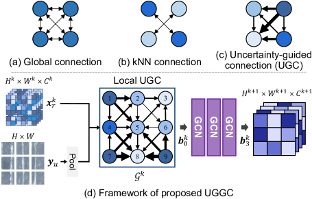
Figure 3: Illustration of three edge connection strategies: (a) global connection, (b) k-nearest neighbor connection, and our (c) Uncertainty-Guided Connection (UGC). (d) Framework of the proposed UGGC based on the local UGC.

In the specific pipeline of UGGC, we first divide the input feature maps $\boldsymbol{x}_{r}^{k}$ and uncertainty map $\boldsymbol{y}_{u}$ into patches of size $n_{p}\times n_{p}$, where $k=1,2,3,4$. To explicitly control the information flow among regions, we constructed a local directed weighted graph $\mathcal{G}^{k}(\mathcal{N}^{k},\mathbf{A}^{k})$ using the proposed local UGC strategy. The node set $\mathcal{N}^{k}$ contains $H_{n}^{k}\times W_{n}^{k}=H^{k}/n_{p}\times W^{k}/n_{p}$ nodes, each node representing a corresponding patch of $\boldsymbol{x}_{r}^{k}$. The feature value of each node is the average pooled feature value of the corresponding patch. The number of channels for each node are consistent with $\boldsymbol{x}_{r}^{k}$. We use $\boldsymbol{b}_{0}^{k}\in\mathbb{R}^{(H_{n}^{k}\times W_{n}^{k})\times C^{k}}$ to represent the initial node features of $\mathcal{N}^{k}$.

To construct the edge set $\mathbf{A}^{k}$, we first calculate an initial directed weighted adjacency matrix $\mathbf{E}^{k}$. The edge weight between nodes $\mathcal{N}^{k}_{i}$ and $\mathcal{N}^{k}_{j}$ is calculated as Eq. (1).

$$\mathbf{E}^{k}_{i,j}=\left\{\begin{aligned} \boldsymbol{y}_{u}^{k}(j)-\boldsymbol{y}_{u}^{k}(i)&,&\boldsymbol{y}_{u}^{k}(i)<\boldsymbol{y}_{u}^{k}(j),\\ 0&,&\boldsymbol{y}_{u}^{k}(i)\geq\boldsymbol{y}_{u}^{k}(j),\end{aligned}\right.$$ (1)

where $\boldsymbol{y}_{u}^{k}(\cdot)$ represents the average uncertainty of pixels within the corresponding patch in UGGC. As presented in Eq. (2), $\mathbf{A}^{k}$ is derived by adding the local constraint to $\mathbf{E}^{k}$.

$$\mathbf{A}^{k}_{i,j}=\left\{\begin{aligned} \mathbf{E}^{k}_{i,j}&,&\lvert i-j\rvert<1\textrm{ and }\lvert r(i)-r(j)\rvert<1,\\ 0&,&\textrm{otherwise},\end{aligned}\right.$$ (2)

where $r(\cdot)$ is the row index of the input node. Following the construction of $\mathcal{G}_{k}$ are three serially connected Graph Convolution Networks (GCNs) (Kipf and Welling 2017). Under the local UGC constraints, the GCNs can regulate the information transmits from confident nodes to uncertain nodes. The specific calculation process is shown as Eq. (3).

$$\boldsymbol{b}_{\ell}^{k}=\tilde{\mathbf{D}^{k}}^{-\frac{1}{2}}\tilde{\mathbf{A}^{k}}\tilde{\mathbf{D}^{k}}^{-\frac{1}{2}}\boldsymbol{b}^{k}_{\ell-1}\mathbf{T}_{\ell},$$ (3)

where $\boldsymbol{b}^{k}_{\ell}\in\mathbb{R}^{(H_{n}^{k}\times W_{n}^{k})\times C_{\ell}^{k}},\ell=1,2,3$ is the input feature map, $\tilde{\mathbf{A}^{k}}=\mathbf{A}^{k}+\mathbf{I}$ is the adjacency matrix added with an identity matrix $\mathbf{I}$, $\tilde{\mathbf{D}^{k}}$ denotes the diagonal node degree matrix of $\tilde{\mathbf{A}^{k}}$, and $\mathbf{T}_{\ell}\in\mathbb{R}^{C_{\ell-1}^{k}\times C_{\ell}^{k}}$ is a learnable weight matrix of the $\ell$-th GCN. To ensure the size and the number of channels of the output features from UGGC match those of the corresponding ResNet encoder, we let $H_{n}^{k}=H_{k+1}$, $W_{n}^{k}=W_{k+1}$, $C_{1}^{k}=C^{k}$, and $C_{2}^{k}=C_{3}^{k}=C^{k+1}$.

UEMA: Uncertainty-Enhanced Manipulation Attention.

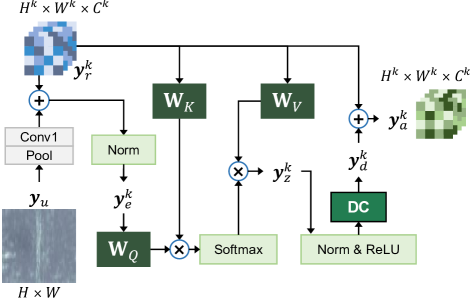
Figure 4: Framework of UEMA. ‘DC’ is short for a depth-wise convolution layer.

In the decoding phase, our goals are to direct more attention towards uncertain regions and align the features of spliced areas while ensuring their distinction from pristine areas. To achieve these two goals simultaneously, we propose the UEMA module (see Fig. 4), which fully leverages the uncertainty map and robust features refined by UGGC to further enhance network performance. Due to the robust feature representation extracted by the UGGC, global correlation computations in UEMA during the decoding phase will not mislead the learning process. We first use uncertainty maps to enhance feature maps and perform cross-attention on the feature maps before and after enhancement. Then, we adopt depth-wise convolution layers to adaptively adjust the weight of each channel to assist in refining.

Taking $\boldsymbol{y}_{r}^{(k)}$ and $\boldsymbol{y}_{u}$ as the input of UEMA, we sequentially perform average pooling and a convolution layer with $1\!\times\!1$ kernels, making the size of $\boldsymbol{y}_{u}$ consistent with $\boldsymbol{y}_{r}^{k}$. Their output can be represented as Eq. (4).

$$\boldsymbol{y}_{e}^{k}=\mathrm{BN}(\boldsymbol{y}_{r}^{k}+\mathrm{Conv1}(\mathrm{AveragePool}(\boldsymbol{y}_{u}))),$$ (4)

where $\mathrm{BN}(\cdot)$ is batch normalization, which is used to normalize the feature map enhanced by the uncertainty map.

$$\boldsymbol{y}_{z}^{k}=\mathrm{Softmax}(\frac{\mathbf{W}^{k}_{Q}(\boldsymbol{y}_{e}^{k})\mathbf{W}^{k}_{K}(\boldsymbol{y}_{r}^{k})^{\intercal}}{\sqrt{d^{k}}})\mathbf{W}^{k}_{V}(\boldsymbol{y}_{r}^{k}),$$ (5)

where $\mathbf{W}^{k}_{Q}(\cdot)$, $\mathbf{W}^{k}_{K}(\cdot)$, $\mathbf{W}^{k}_{V}(\cdot)\in\mathbb{R}^{d^{k}\times d^{k}}$ are the linear projections corresponding to the query, key, and value, respectively. Here, $d^{k}=H^{k}\times W^{k}$ denotes the number of pixels in a single feature map. Using $\boldsymbol{y}_{e}^{k}$ as the query, the UEMA can be essentially instructed to focus its attention on these areas of uncertain regions and regions suspected of splicing. In addition, $\boldsymbol{y}_{r}^{k}$ serves as the key and value, providing the original basis for global correlation computing. Lastly, acknowledging the different contributions from various channels towards the rectification of weakly predicted regions, we incorporate three cascaded depth-wise convolution layers $\mathrm{DC}(\cdot)$ (with kernel sizes of $3\!\times\!3$) (Chen et al. 2022) to further refine $\boldsymbol{y}_{v}^{k}$, allowing for an adaptive adjustment of weights among the channel dimension.

$$\boldsymbol{y}_{a}^{k}=\boldsymbol{y}_{z}^{k}+\mathrm{DC}(\mathrm{BN}(\mathrm{ReLU}(\boldsymbol{y}_{v}^{k}))).$$ (6)

4.4 Loss Functions

To simultaneously enhance pixel-level and image-level detection capabilities, we follow previous works (Dong et al. 2023) to combine classification and segmentation loss. Regarding the segmentation loss $L_{seg}$, we employ a combination of binary cross entropy (BCE) and Dice in each stage. The proportion of background pixels far exceeds that of spliced pixels, thus we choose Dice loss with its capability in dealing with imbalanced samples (Lin et al. 2023; Dong et al. 2023). For classification loss $L_{cls}$, we supervise the maximum value of predicted binary mask $\boldsymbol{y}_{v}$ to suppress false alarms. These loss functions are formulated as follows.

$$L_{seg}=\gamma_{b}\cdot L_{bce}(\boldsymbol{y}_{v},\boldsymbol{y})+\gamma_{d}\cdot L_{dice}(\boldsymbol{y}_{v},\boldsymbol{y}),\\$$ (7)

$$L_{cls}=L_{bce}(\mathrm{max}_{p}(\boldsymbol{y}_{v}),\mathrm{max}_{p}(\boldsymbol{y})),\\$$ (8)

$$L_{total}=\gamma_{s}\cdot L_{seg}+\gamma_{c}\cdot L_{cls},\\$$ (9)

where $\boldsymbol{y}\in\left\{0,1\right\}^{H\times W}$ is the pixel-level ground truth, with 1 indicating a spliced pixel and 0 pointing to a pristine one. The function $\textrm{max}_{p}(\cdot)$ can calculate the maximum element value of the two-dimensional input tensor. The empirical parameters $\gamma_{b},\gamma_{d},\gamma_{s}$ denote the loss weight adjusting factors. Note that $L_{total}$ is used for both two stages of URN.

Table 2: Pixel-level (i.e., F1 and MCC) and image-level (i.e., AUC and Acc, marked in gray) performance (%) of biomedical image splicing detection. The first and second rankings are respectively shown in bold and underlined. Note that ‘ManTra’ represents the results shown in Biofors (Sabir et al. 2021), whereas ‘ManTra*’ denotes the results we reproduce.

Method	Venue		Biofors					RSIID					BioSp-C					BioSp-H					Average
			F1	MCC	AUC	Acc		F1	MCC	AUC	Acc		F1	MCC	AUC	Acc		F1	MCC	AUC	Acc		F1	MCC	AUC	Acc
RRU-Net	CVPRW 19		14.9	14.9	79.9	75.5		80.6	80.4	99.1	94.0		31.9	32.7	83.0	73.3		32.4	32.8	76.1	68.0		40.0	40.2	83.4	77.7
ManTra*	CVPR 19		12.4	8.0	55.3	50.0		48.8	49.9	98.4	84.1		20.7	21.3	73.8	63.4		0.4	-0.1	54.8	59.8		20.6	20.9	69.2	64.3
ManTra	CVPR 19		9.0	8.0	-	-		-	-	-	-		-	-	-	-		-	-	-	-		-	-	-	-
GSR-Net	AAAI 20		3.1	2.4	70.3	65.7		79.1	79.0	98.8	93.3		21.7	22.2	73.4	65.8		23.6	23.4	71.1	66.8		31.9	31.9	77.2	72.9
MVSS	TPAMI 23		11.4	10.9	77.8	60.0		77.3	77.2	99.3	95.1		15.8	16.2	79.9	64.2		29.0	29.0	76.7	66.8		33.4	33.5	79.0	71.5
IF-OSN	CVPR 22		9.6	8.7	72.8	66.7		80.1	80.0	98.9	95.1		14.3	13.5	76.7	69.8		12.5	12.0	65.3	58.0		29.1	28.8	76.9	72.4
PSCC-Net	TCSVT 22		12.9	7.0	71.2	63.0		70.1	70.3	99.5	95.4		6.5	1.5	79.4	68.0		18.3	14.7	61.9	31.2		27.0	24.9	76.0	64.4
CAT-Net 2	IJCV 22		13.8	12.4	59.8	53.7		77.4	77.1	97.9	91.2		22.9	23.0	76.8	69.8		30.4	30.3	74.6	64.0		36.1	36.1	75.8	69.7
TruFor	CVPR 23		8.3	8.9	71.4	66.7		77.3	77.5	99.3	94.7		17.5	17.6	75.8	64.0		19.7	19.6	74.0	65.3		30.7	30.8	79.0	72.7
Hifi	CVPR 23		21.7	20.1	66.7	61.1		77.4	77.2	98.7	84.5		35.8	37.7	77.2	72.7		26.2	26.0	66.8	69.0		40.3	40.7	75.9	71.8
URN	Ours		30.3	30.4	87.8	75.0		81.4	81.4	99.3	94.9		38.5	39.3	85.9	75.0		38.9	38.9	78.0	68.7		47.3	47.5	84.6	78.4

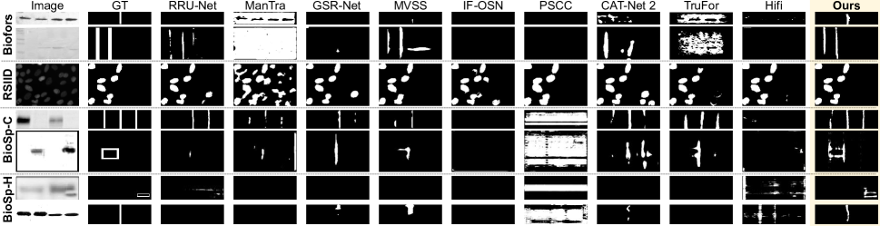
Figure 5: Qualitative results over Biofors, RSIID, BioSp-C, and BioSp-H. From left to right, each column represents images, ground truth labels (GT), and predictions of selected SoTAs, respectively.

5 Experimental Results

In this section, we provide descriptions of the experiment setups, comparative experiment results, and compact ablation studies. Due to the space limitations, more experimental results, i.e., the cross-dataset testing, robustness analysis, and performance of natural image manipulation detection, are provided in the supplementary material.

5.1 Experiment Setups

Datasets. In addition to our two sub-datasets, i.e., BioSp-C and BioSp-H, we also conduct experiments on two publicly available biomedical datasets, i.e., Biofors (cut/sharp-transition part) and RSIID (splicing part), that are applicable for splicing detection. To prevent the interference of false negatives, we randomly sample pristine images from Biofors for BioSp. We ensure that there is no overlap in the selection of pristine images among Biofors, BioSp-C, and BioSp-H. To avoid biases due to imbalanced data, we sample pristine images to ensure their quantity is equal to spliced ones. Note that we select a training-testing ratio of 7:3 for each dataset.

Evaluation Metrics. Following previous works (Guillaro et al. 2023; Dong et al. 2023), we use F1-score and Matthews Correlation Coefficient (MCC) to evaluate pixel-level results. Besides, we utilize Area Under the receiver operating characteristic Curve (AUC) and accuracy (Acc) as metrics for image-level detection. For fair comparisons, we set the default decision thresholds of F1, MCC, and Acc to 0.5.

5.2 Comparison with SoTAs

Since there is no deep learning-based method proposed for this task, we select SoTA image manipulation or splicing detection methods designed for natural image. Selected methods drop into two categories: (1) noise-sensitive methods, including ManTra (Wu, AbdAlmageed, and Natarajan 2019), MVSS (Dong et al. 2023) and TruFor (Guillaro et al. 2023), (2) noise-insensitive methods, i.e., RRU-Net (Bi et al. 2019), GSR-Net (Zhou et al. 2020), IF-OSN (Wu et al. 2022), PSCC-Net (Liu et al. 2022), CAT-Net 2 (Kwon et al. 2022), and Hifi (Guo et al. 2023). All these methods are with publicly available source codes and re-trained on selected datasets. We automatically choose their hyperparameters as described in the corresponding reference papers or optimally assign better ones.

In Tab. 2, we show both pixel-level and image-level detection results. Our method outperforms all SoTAs in terms of average metric values across all datasets, achieving the highest scores in both pixel-level metrics for each dataset. Besides, half of the image-level metric values of URN rank second. As we can see in Fig. 5, our method has lower false alarms and is more capable of accurately localizing subtle splicing traces. This indicates the effectiveness of our strategy of using uncertainty information to refine predictions.

Table 3: Ablation results (%) on BioSp-C. Columns ‘L’, ‘D’, and ‘W’ denote whether the edge connection strategy used in the graph construction of UGGC is local, directed, and weighted, respectively. The decoding components ‘SA’, ‘CA’, and ‘DC’ is short for the self-attention, cross-attention, and depth-wise convolution, respectively.

Case	Refine	Stage 2 Refinement Component					Metric Value
		Encode				Decode
		Module	L	D	W	Module	F1	MCC
1	✕	-	-	-	-	-	30.4	31.9
2	✓	-	-	-	-	UEMA	32.0	34.5
3	✓	UGGC (kNN)	-	✓	✕	UEMA	30.0	31.0
4	✓	UGGC	✓	✕	✕	UEMA	21.6	22.6
5	✓	UGGC	✓	✓	✕	UEMA	33.8	35.3
6	✓	SA	✕	✕	✕	UEMA	32.5	34.9
7	✓	UGGC	✕	✓	✕	UEMA	33.2	34.3
8	✓	UGGC	✕	✓	✓	UEMA	35.8	37.0
9	✓	UGGC	✓	✓	✓	-	32.5	33.6
10	✓	UGGC	✓	✓	✓	SA	35.0	35.5
11	✓	UGGC	✓	✓	✓	CA	29.0	30.4
12	✓	UGGC	✓	✓	✓	DC	34.6	35.6
13	✓	UGGC+UEMA	✓	✓	✓	UEMA	36.9	37.3
14	✓	UGGC+UEMA	✓	✓	✓	-	34.6	35.5
Full	✓	UGGC	✓	✓	✓	UEMA	38.5	39.3

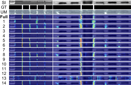
Figure 6: Feature visualization of ablation study. From top to bottom, each row respectively represents the spliced images (SI), ground truth (GT), uncertainty maps (UM), and feature heatmaps of the corresponding case.

5.3 Ablation Study

In Tab. 3, we present the specific configurations and performance of different variants by replacing or removing key components. To further confirm the regions each case tends to focus, we show feature visualization results of all variants using Grad-CAM (Selvaraju et al. 2020) in Fig. 6.

Effectiveness of the Two-Stage Framework. From the row UM in Fig. 6, it can be seen that the uncertainty maps we estimated in the stage-1 network effectively identify regions prone to erroneous prediction due to disruptive factors. As shown in Tab. 3, the metric values of Case 1 are lower than most of the other cases. Additionally, from the 4-th in Fig. 6, we can see that Case 1 losses focus on some spliced regions and incorrectly attends to pristine areas.

Effectiveness of the UGGC. As shown in Tab. 3, we observe that adding UGGC modules (compare Case 2 with Full) brings a 6.5% and 4.8% increase in F1 and MCC, respectively. Also, it helps to reduce the erroneous attention to non-spliced regions with high uncertainty (see Fig. 6). Additionally, in Cases 3-8, we investigate the impact of different edge connection strategies for the construction of $\mathcal{G}^{k}$ in UGGC, including the scope of edge connection, and whether the edges are directed and weighted. As shown in Tab. 3, regardless of the type of involved edge connection strategy used, all resulted in a decrease in performance compared to the proposed strategy. This demonstrates that restricting the information flow from confident nodes to local uncertain ones can help weak-predicted regions capture local inconsistency from nearby areas, thereby enhancing robustness.

Effectiveness of the UEMA. As shown in Tab. 3 and Fig. 6, we explored the effectiveness of UEMA by constructing Cases 9-12. Whether UEMA is removed or replaced with self-attention, cross-attention, or depth-wise convolution, none can achieve better performance. It should be noted that the metric values of Case 11 drop, indicating that a semantic gap exists between estimated uncertainty maps and features in deep layers. Directly calculating their correlation would mislead the decoding process. This also demonstrates that our strategy of enhancing feature maps with uncertainty maps can help UEMA in focusing on uncertain regions and distinguish between spliced and pristine areas.

To further explore the effectiveness of UEMA in different positions of our URN, we give a comparison among Cases 13, 14, and Full in Tab. 3 and Fig. 6. We testify two variants: Case 13 with UEMA in both the decoding and encoding stages, and Case 14 with UEMA only in the encoding stage. We observe that the performance of Case 13 is inferior to Case Full, suggesting that the unrestricted global information transition in UEMA interferes with the robust features refined by UGGC during encoding. Moreover, the performance of Case 14 is even worse than Case 13, implying that additional attention to uncertain regions is effective during the decoding stage.

6 Conclusion

In this paper, we propose an end-to-end Uncertainty-guided Refinement Network (URN) for biomedical image splicing detection. URN is able to identify uncertainly predicted regions and regulate the direction and intensity of information flow between uncertain regions and confident ones. It also can direct the attention to refine uncertainly predicted regions. These proposed strategies allow URN to be resilient to disruptive factors present in biomedical images. Comprehensive experimental results demonstrate that our method outperforms SoTAs designed for natural image manipulation detection. The construction of our BioSp dataset also shows the potential to drive advancements in this field.

References

- Bi et al. (2019) Bi, X.; Wei, Y.; Xiao, B.; and Li, W. 2019. RRU-Net: The Ringed Residual U-Net for Image Splicing Forgery Detection. In IEEE/CVF Computer Vision and Pattern Recognition Conference (CVPR) Workshop, 30–39.
- Bi et al. (2023) Bi, X.; Yan, W.; Liu, B.; Xiao, B.; Li, W.; and Gao, X. 2023. Self-Supervised Image Local Forgery Detection by JPEG Compression Trace. In AAAI Conference on Artificial Intelligence (AAAI), 232–240.
- Bik, Casadevall, and Fang (2016) Bik, E. M.; Casadevall, A.; and Fang, F. C. 2016. The prevalence of inappropriate image duplication in biomedical research publications. MBio, 7(3): e00809–16.
- Binh and Woo (2022) Binh, L. M.; and Woo, S. S. 2022. ADD: Frequency Attention and Multi-View Based Knowledge Distillation to Detect Low-Quality Compressed Deepfake Images. In AAAI Conference on Artificial Intelligence (AAAI), 122–130.
- Bucci (2018) Bucci, E. M. 2018. Automatic detection of image manipulations in the biomedical literature. Cell Death & Disease, 9(3): 1–9.
- Cardenuto and Rocha (2022) Cardenuto, J. P.; and Rocha, A. 2022. Benchmarking Scientific Image Forgery Detectors. Sci. Eng. Ethics, 28(4): 35.
- Chen et al. (2022) Chen, Q.; Wu, Q.; Wang, J.; Hu, Q.; Hu, T.; Ding, E.; Cheng, J.; and Wang, J. 2022. MixFormer: Mixing Features across Windows and Dimensions. In IEEE/CVF Computer Vision and Pattern Recognition Conference (CVPR), 5239–5249.
- Cozzolino and Verdoliva (2020) Cozzolino, D.; and Verdoliva, L. 2020. Noiseprint: A CNN-Based Camera Model Fingerprint. IEEE Trans. Inf. Forensics Secur. (TIFS), 15: 144–159.
- Dong et al. (2023) Dong, C.; Chen, X.; Hu, R.; Cao, J.; and Li, X. 2023. MVSS-Net: Multi-View Multi-Scale Supervised Networks for Image Manipulation Detection. IEEE Trans. Pattern Anal. Mach. Intell. (TPAMI), 45(3): 3539–3553.
- Guillaro et al. (2023) Guillaro, F.; Cozzolino, D.; Sud, A.; Dufour, N.; and Verdoliva, L. 2023. TruFor: Leveraging all-round clues for trustworthy image forgery detection and localization. In IEEE/CVF Computer Vision and Pattern Recognition Conference (CVPR).
- Guo et al. (2023) Guo, X.; Liu, X.; Ren, Z.; Grosz, S.; Masi, I.; and Liu, X. 2023. Hierarchical Fine-Grained Image Forgery Detection and Localization. In IEEE/CVF Computer Vision and Pattern Recognition Conference (CVPR).
- Han et al. (2022) Han, K.; Wang, Y.; Guo, J.; Tang, Y.; and Wu, E. 2022. Vision GNN: An Image is Worth Graph of Nodes. In Conference on Neural Information Processing Systems (NeuralIPS).
- Hao et al. (2021) Hao, J.; Zhang, Z.; Yang, S.; Xie, D.; and Pu, S. 2021. TransForensics: Image Forgery Localization with Dense Self-Attention. In IEEE/CVF International Conference on Computer Vision (ICCV), 15035–15044.
- Hu et al. (2020) Hu, X.; Zhang, Z.; Jiang, Z.; Chaudhuri, S.; Yang, Z.; and Nevatia, R. 2020. SPAN: Spatial Pyramid Attention Network for Image Manipulation Localization. In European Conference on Computer Vision (ECCV), 312–328.
- Kendall, Badrinarayanan, and Cipolla (2017) Kendall, A.; Badrinarayanan, V.; and Cipolla, R. 2017. Bayesian SegNet: Model Uncertainty in Deep Convolutional Encoder-Decoder Architectures for Scene Understanding. In The British Machine Vision Conference (BMVC).
- Kipf and Welling (2017) Kipf, T. N.; and Welling, M. 2017. Semi-Supervised Classification with Graph Convolutional Networks. In International Conference on Learning Representations (ICLR).
- Koker et al. (2020) Koker, T. E.; Chintapalli, S. S.; Wang, S.; Talbot, B. A.; Wainstock, D.; Cicconet, M.; and Walsh, M. C. 2020. On Identification and Retrieval of Near-Duplicate Biological Images: a New Dataset and Protocol. In International Conference on Pattern Recognition (ICPR), 3114–3121.
- Kwon et al. (2022) Kwon, M.; Nam, S.; Yu, I.; Lee, H.; and Kim, C. 2022. Learning JPEG Compression Artifacts for Image Manipulation Detection and Localization. Int. J. Comput. Vis. (IJCV), 130(8): 1875–1895.
- Kwon et al. (2021) Kwon, M.; Yu, I.; Nam, S.; and Lee, H. 2021. CAT-Net: Compression Artifact Tracing Network for Detection and Localization of Image Splicing. In IEEE/CVF Winter Conference on Applications of Computer Vision (WACV), 375–384.
- Lin et al. (2023) Lin, X.; Wang, S.; Deng, J.; Fu, Y.; Bai, X.; Chen, X.; Qu, X.; and Tang, W. 2023. Image manipulation detection by multiple tampering traces and edge artifact enhancement. Pattern Recognit., 133: 109026.
- Liu et al. (2022) Liu, X.; Liu, Y.; Chen, J.; and Liu, X. 2022. PSCC-Net: Progressive Spatio-Channel Correlation Network for Image Manipulation Detection and Localization. IEEE Trans. Circuits Syst. Video Technol. (TCSVT), 32(11): 7505–7517.
- Lorch, Maier, and Riess (2020) Lorch, B.; Maier, A.; and Riess, C. 2020. Reliable JPEG Forensics via Model Uncertainty. In IEEE International Workshop on Information Forensics and Security (WIFS), 1–6.
- Maier, Lorch, and Riess (2020) Maier, A.; Lorch, B.; and Riess, C. 2020. Toward Reliable Models For Authenticating Multimedia Content: Detecting Resampling Artifacts With Bayesian Neural Networks. In IEEE International Conference on Image Processing (ICIP), 1251–1255.
- Mandelli et al. (2022) Mandelli, S.; Cozzolino, D.; Cannas, E. D.; Cardenuto, J. P.; Moreira, D.; Bestagini, P.; Scheirer, W. J.; Rocha, A.; Verdoliva, L.; Tubaro, S.; and Delp, E. J. 2022. Forensic Analysis of Synthetically Generated Western Blot Images. IEEE Access, 10: 59919–59932.
- Miura and Nørrelykke (2021) Miura, K.; and Nørrelykke, S. F. 2021. Reproducible image handling and analysis. The EMBO Journal, 40(3): e105889.
- Moreira et al. (2022) Moreira, D.; Cardenuto, J. P.; Shao, R.; Baireddy, S.; Cozzolino, D.; Gragnaniello, D.; Abd-Almageed, W.; Bestagini, P.; Tubaro, S.; Rocha, A.; Scheirer, W.; Verdoliva, L.; and Delp, E. 2022. SILA: a system for scientific image analysis. Scientific Reports, 12(1).
- Rombach et al. (2022) Rombach, R.; Blattmann, A.; Lorenz, D.; Esser, P.; and Ommer, B. 2022. High-Resolution Image Synthesis With Latent Diffusion Models. In IEEE/CVF Computer Vision and Pattern Recognition Conference (CVPR), 10684–10695.
- Rossner and Yamada (2004) Rossner, M.; and Yamada, K. M. 2004. What’s in a picture? The temptation of image manipulation. The Journal of Cell Biology, 166(1): 11–15.
- Sabir et al. (2021) Sabir, E.; Nandi, S.; AbdAlmageed, W.; and Natarajan, P. 2021. BioFors: A Large Biomedical Image Forensics Dataset. In IEEE/CVF International Conference on Computer Vision (ICCV), 10943–10953.
- Sabir et al. (2022) Sabir, E.; Nandi, S.; AbdAlmageed, W.; and Natarajan, P. 2022. MONet: Multi-Scale Overlap Network for Duplication Detection in Biomedical Images. In IEEE International Conference on Image Processing (ICIP), 3793–3797.
- Selvaraju et al. (2020) Selvaraju, R. R.; Cogswell, M.; Das, A.; Vedantam, R.; Parikh, D.; and Batra, D. 2020. Grad-CAM: Visual Explanations from Deep Networks via Gradient-Based Localization. Int. J. Comput. Vis., 128(2): 336–359.
- Shao, Wu, and Liu (2023) Shao, R.; Wu, T.; and Liu, Z. 2023. Detecting and Grounding Multi-Modal Media Manipulation. In IEEE/CVF Computer Vision and Pattern Recognition Conference (CVPR).
- Suvorov et al. (2022) Suvorov, R.; Logacheva, E.; Mashikhin, A.; Remizova, A.; Ashukha, A.; Silvestrov, A.; Kong, N.; Goka, H.; Park, K.; and Lempitsky, V. 2022. Resolution-robust Large Mask Inpainting with Fourier Convolutions. In IEEE/CVF Winter Conference on Applications of Computer Vision (WACV), 3172–3182.
- Verdoliva (2020) Verdoliva, L. 2020. Media Forensics and DeepFakes: An Overview. IEEE J. Sel. Top. Signal Process., 14(5): 910–932.
- Wang et al. (2022) Wang, J.; Wu, Z.; Chen, J.; Han, X.; Shrivastava, A.; Lim, S.; and Jiang, Y. 2022. ObjectFormer for Image Manipulation Detection and Localization. In IEEE/CVF Computer Vision and Pattern Recognition Conference (CVPR), 2354–2363.
- Wu et al. (2022) Wu, H.; Zhou, J.; Tian, J.; and Liu, J. 2022. Robust Image Forgery Detection over Online Social Network Shared Images. In IEEE/CVF Computer Vision and Pattern Recognition Conference (CVPR), 13430–13439.
- Wu, AbdAlmageed, and Natarajan (2019) Wu, Y.; AbdAlmageed, W.; and Natarajan, P. 2019. ManTra-Net: Manipulation Tracing Network for Detection and Localization of Image Forgeries With Anomalous Features. In IEEE/CVF Computer Vision and Pattern Recognition Conference (CVPR), 9543–9552.
- Zheng et al. (2021) Zheng, E.; Yu, Q.; Li, R.; Shi, P.; and Haake, A. R. 2021. A Continual Learning Framework for Uncertainty-Aware Interactive Image Segmentation. In AAAI Conference on Artificial Intelligence (AAAI), 6030–6038.
- Zhou et al. (2020) Zhou, P.; Chen, B.; Han, X.; Najibi, M.; Shrivastava, A.; Lim, S.; and Davis, L. 2020. Generate, Segment, and Refine: Towards Generic Manipulation Segmentation. In AAAI Conference on Artificial Intelligence (AAAI), 13058–13065.
- Zhou et al. (2018) Zhou, P.; Han, X.; Morariu, V. I.; and Davis, L. S. 2018. Learning Rich Features for Image Manipulation Detection. In IEEE/CVF Computer Vision and Pattern Recognition Conference (CVPR), 1053–1061.
- Zhuang et al. (2021) Zhuang, P.; Li, H.; Tan, S.; Li, B.; and Huang, J. 2021. Image Tampering Localization Using a Dense Fully Convolutional Network. IEEE Trans. Inf. Forensics Secur. (TIFS), 16: 2986–2999.