Streaming quantum state purification

Abstract

Quantum state purification is the task of recovering a nearly pure copy of an unknown pure quantum state using multiple noisy copies of the state. This basic task has applications to quantum communication over noisy channels and quantum computation with imperfect devices, but has only been studied previously for the case of qubits. We derive an efficient purification procedure based on the swap test for qudits of any dimension, starting with any initial error parameter. Treating the initial error parameter and the dimension as constants, we show that our procedure has sample complexity asymptotically optimal in the final error parameter. Our protocol has a simple recursive structure that can be applied when the states are provided one at a time in a streaming fashion, requiring only a small quantum memory to implement.

1 Introduction

Quantum states are notoriously susceptible to the effects of decoherence. Thus, a basic challenge in quantum information processing is to find ways of protecting quantum systems from noise, or of removing noise that has already occurred. In this paper we study the latter approach, aiming to (partially) reverse the effect of decoherence and produce less noisy states out of mixed ones, a process that we call purification.

Since noise makes quantum states less distinguishable, it is impossible to purify a single copy of a noisy state. However, given multiple copies of a noisy state, we can try to reconstruct a single copy that is closer to the original pure state. In general, we expect the quality of the reconstructed state to be higher if we are able to use more copies of the noisy state. We would like to understand the number of samples that suffice to produce a high-fidelity copy of the original state, and to give efficient procedures for carrying out such purification.

More precisely, we focus on depolarizing noise and consider the following formulation of the purification problem. Let $|{\psi}\rangle\in\mathbb{C}^{d}$ be an unknown pure $d$-dimensional state (or qudit). In the qudit purification problem, we are given multiple noisy copies of $|{\psi}\rangle$ that are all of the form

$$\rho(\delta):=(1-\delta)|{\psi}\rangle\langle{\psi}|+\delta\,\frac{I}{d},$$ (1)

where the error parameter $\delta\in(0,1)$ represents the probability that the state is depolarized. If we need to compare error parameters across different dimensions, we write $\delta^{(d)}$ to specify the underlying dimension.

Let $\mathcal{P}$ denote a purification procedure, which is a quantum operation that maps $N$ copies of $\rho(\delta)$ to a single qudit. (Note that the implementation of $\mathcal{P}$ can make use of additional quantum workspace.) We refer to $N$ as the sample complexity of $\mathcal{P}$. The goal is to produce a single qudit that closely approximates the desired (but unknown) target state $|{\psi}\rangle$. In particular, we aim to produce a state whose fidelity with the ideal pure state $|{\psi}\rangle$ is within some specified tolerance, using the smallest possible sample complexity $N$. Our streaming protocol produces a state of the form $\rho(\epsilon)$ for some small $\epsilon>0$, which has fidelity $1-(1-\frac{1}{d})\epsilon$ with $|{\psi}\rangle$, so it is convenient to focus on the output error parameter $\epsilon$.

The purification problem was first studied over two decades ago. Inspired by studies of entanglement purification [BBP⁺96], Cirac, Ekert, and Macchiavello studied the problem of purifying a depolarized qubit and found the optimal purification procedure [CEM99]. Later, Keyl and Werner studied qubit purification under different criteria, including the possibility of producing multiple copies of the output state and measuring the fidelity either by comparing a single output state or selecting all the output states [KW01]. However, little was known about how to purify higher-dimensional quantum states.

Our main contribution is the first concrete and efficient qudit purification procedure, which achieves the following.

Theorem 1 (Informal).

For any fixed input error parameter $\delta\in(0,1)$, there is a protocol that produces a state with output error parameter at most $\epsilon\in(0,1)$ using $O(1/\epsilon)$ samples of the $d$-dimensional input state and $O(\frac{1}{\epsilon}\log d)$ elementary gates.

We present this protocol in Section 2 and analyze its performance in Section 3, establishing a formal version of the above result (Theorem 9 and Corollary 11).

As an application, in Section 4 we use our procedure to solve a version of Simon’s problem with a faulty oracle. In particular, we show that if the oracle depolarizes its output by a constant amount, then the problem can still be solved with only quadratic overhead, preserving the exponential quantum speedup.

Rather than applying Schur–Weyl duality globally as in [CEM99], our streaming purification protocol recursively applies the swap test to pairs of quantum states. This approach has two advantages. First, our procedure readily works for quantum states of any dimension. Second, the swap test is much easier to implement and analyze than a general Schur basis measurement. In particular, the protocol can be implemented in a scenario where the states arrive in an online fashion, using a quantum memory of size only logarithmic in the total number of states used.

Since our protocol does not respect the full permutation symmetry of the problem, it is not precisely optimal. However, suppose we fix the dimension and the initial error parameter. Then, in the qubit case, our sample complexity matches that of the optimal protocol [CEM99] up to factors involving these constants, suggesting that the procedure performs well. Furthermore, in Section 5 we prove a lower bound showing that our protocol has optimal scaling in the final error parameter up to factors involving the other constants. Whether our protocol remains asymptotically optimal when the dimension is not necessarily constant is left as an open problem.

The optimal purification protocol should respect the permutation symmetry of the input and hence can be characterized using Schur–Weyl duality. Some of the authors have developed a framework for studying such optimal purification procedures, although this has not yet led to a full characterization of the optimal protocol. We briefly describe this related work in Section 6 along with a summary of the results and a discussion of some other open questions.

Purification is closely related to the following quantum majority vote problem [BLM⁺22]: given an $N$-qubit state $U^{\otimes N}|{x}\rangle$ for an unknown unitary $U\in\mathrm{U}(2)$ and bit string $x\in\{0,1\}^{N}$, output an approximation of $U\,|{\mathrm{MAJ}(x)}\rangle$, where $\mathrm{MAJ}(x)\in\{0,1\}$ denotes the majority of $x$. While the input to this problem is not of the form $\rho^{\otimes N}$, applying a random permutation produces a separable state whose single-qubit marginals are identical and equal to a state $\rho$ given in eq. 1. The optimal quantum majority vote procedure for qubits is known [BLM⁺22] and seems to coincide with the optimal qubit purification procedure [CEM99]. However, its generalization to qudits has been investigated only in very limited cases [GO23].

2 Purification using the swap test

In this section, we present a recursive purification procedure based on the swap test. We review the swap test in Section 2.1 and define a gadget that uses it to project onto the symmetric subspace in Section 2.2. In Section 2.3, we describe how this gadget acts on depolarized copies of a pure state, and in Section 2.4, we specialize to the case where the two input copies have the same purity. We then define our recursive purification procedure in Section 2.5. Finally, we describe a stack-based implementation of this procedure in Section 2.6, providing a bound on the space complexity.

2.1 The swap test

The swap test is a standard procedure for comparing two unknown quantum states [BCWDW01]. It takes two input states $\rho$ and $\sigma$ of the same dimension, and requires one ancilla qubit initialized to $|{0}\rangle$ (see Fig. 1). The outcome $a\in\{0,1\}$ of the measurement on the ancilla qubit indicates whether the states $\rho$ and $\sigma$ are close to each other ($a=0$) or close to being orthogonal ($a=1$). While often one is interested only in this classical output, the swap test also produces two potentially entangled quantum registers that contain a particular $a$-dependent combination of $\rho$ and $\sigma$.

Figure 1: Quantum circuit for the swap test on arbitrary input states $\rho$ and $\sigma$. The gate in the middle denotes the controlled-swap operation while $H=\frac{1}{\sqrt{2}}\bigl{(}\begin{smallmatrix}1&\phantom{-}1\\ 1&-1\end{smallmatrix}\bigr{)}$ is the Hadamard gate.

Our purification algorithm keeps only one of the two quantum output registers, so let us derive an expression for the output state $\omega(a)$ on the first qudit. Note that the control qubit is prepared in the state $H|{0}\rangle=\frac{|{0}\rangle+|{1}\rangle}{\sqrt{2}}$ and then measured in the Hadamard basis $\frac{|{0}\rangle\pm|{1}\rangle}{\sqrt{2}}$. We can use the identity

(2)

to eliminate this qubit and replace the controlled-swap gate $|{0}\rangle\langle{0}|\otimes I+|{1}\rangle\langle{1}|\otimes S$ with a linear combination of the identity gate $I$ and the swap gate $S\colon|{i}\rangle\otimes|{j}\rangle\mapsto|{j}\rangle\otimes|{i}\rangle$ on the last two registers.

For a given measurement outcome $a\in\{0,1\}$ in Fig. 1, the corresponding sub-normalized post-measurement state on the last two registers is

$$\frac{I+(-1)^{a}S}{2}(\rho\otimes\sigma)\frac{I+(-1)^{a}S}{2},$$ (3)

where $\frac{1}{2}(I+S)$ and $\frac{1}{2}(I-S)$ project onto the symmetric and the anti-symmetric subspace, respectively. Discarding the last register yields the sub-normalized state

$$\frac{1}{4}\big{\lparen}\rho+\sigma+(-1)^{a}\rho\sigma+(-1)^{a}\sigma\rho\big{\rparen},$$ (4)

where the last two terms are obtained from the identity

(5)

Since the probability of obtaining outcome $a$ is given by the trace

$$\frac{1}{2}\big{\lparen}1+(-1)^{a}\operatorname{Tr}(\rho\sigma)\big{\rparen}$$ (6)

of eq. 4, the normalized output state $\omega(a)$ in Fig. 1 is

$$\omega(a)=\frac{1}{2}\cdot\frac{\rho+\sigma+(-1)^{a}(\rho\sigma+\sigma\rho)}{1+(-1)^{a}\operatorname{Tr}(\rho\sigma)}.$$ (7)

Note that the swap test can be implemented with $O(\log d)$ quantum gates since a swap gate between qudits can be decomposed into swaps of constituent qubits.

2.2 The swap test gadget

We are particularly interested in the output state $\omega(0)$ that corresponds to the measurement outcome $a=0$. This state is equal to the normalized projection of $\rho\otimes\sigma$ onto the symmetric subspace. Algorithm 1 introduces a Swap gadget that performs the swap test on fresh copies of the input states $\rho$ and $\sigma$ until it succeeds in obtaining the $a=0$ outcome.

Algorithm 1 Swap gadget.

This procedure has access to a stream of inputs $\rho$ and $\sigma$, and uses as many copies of them as necessary.

1: procedure Swap($\rho,\sigma$)

2:      repeat

3:          Ask for one fresh copy of $\rho$ and $\sigma$.

4:          Apply the swap test shown in Fig. 1 and denote the measurement outcome by $a$.

5:      until $a=0$

6:      return the state $\omega(0)$ of the output register

We denote the final output of the Swap gadget by

$$\textsc{Swap}(\rho,\sigma):=\frac{1}{2}\cdot\frac{\rho+\sigma+\rho\sigma+\sigma\rho}{1+\operatorname{Tr}(\rho\sigma)},$$ (8)

which is just $\omega(0)$ from eq. 7. The expected number of copies of each input state consumed by this gadget is given by the inverse of its success probability. By eq. 6, this is $2/\lparen 1+\operatorname{Tr}(\rho\sigma)\rparen$.

2.3 Output error parameter as a function of input errors

For the purpose of purification, we are particularly interested in the special case when both input states, $\rho$ and $\sigma$, are of the form

$$\rho(\delta):=(1-\delta)|{\psi}\rangle\langle{\psi}|+\delta\,\frac{I}{d}$$ (9)

for some error parameter $\delta\in(0,1)$, where $|{\psi}\rangle\in\mathbb{C}^{d}$ is an unknown but fixed $d$-dimensional state (the dimension $d\geq 2$ is often implicit). The following claim shows that the Swap gadget (Algorithm 1) preserves the form of these states, irrespective of the actual state $|{\psi}\rangle$, and derives the error parameter of the output state as a function of both input error parameters.

Claim 2.

If the input states of Algorithm 1 are $\rho(\delta_{1})$ and $\rho(\delta_{2})$ as described in eq. 9, then

$$\textsc{Swap}\big{\lparen}\rho(\delta_{1}),\rho(\delta_{2})\big{\rparen}=\rho(\delta^{\prime})\qquad\text{where}\qquad\delta^{\prime}:=\frac{\frac{\delta_{1}+\delta_{2}}{2}+\frac{\delta_{1}\delta_{2}}{d}}{(1+\frac{1}{d})+(1-\frac{1}{d})(1-\delta_{1})(1-\delta_{2})}.$$ (10)

Proof.

Equation 9 shows that both input states are linear combinations of projectors $\{|{\psi}\rangle\langle{\psi}|,I\}$. Since this set is closed under matrix multiplication, the output state in eq. 8 is also a linear combination of $|{\psi}\rangle\langle{\psi}|$ and $I$. By construction, the output is positive semi-definite and has unit trace, so it must be of the form $\rho(\delta^{\prime})$ for some $\delta^{\prime}\in[0,1]$.

Note that $\rho(\delta_{1})$ and $\rho(\delta_{2})$ are diagonal in the same basis, so $\rho(\delta_{1})\rho(\delta_{2})=\rho(\delta_{2})\rho(\delta_{1})$ and hence the numerator of eq. 8 is $\rho(\delta_{1})+\rho(\delta_{2})+2\rho(\delta_{1})\rho(\delta_{2})$. Using eq. 9, the coefficient of $I$ in this expression is

$$\alpha:=\frac{\delta_{1}}{d}+\frac{\delta_{2}}{d}+2\frac{\delta_{1}\delta_{2}}{d^{2}}.$$ (11)

The denominator of eq. 8 is given by

$$\beta :=1+\operatorname{Tr}\big{\lparen}\rho(\delta_{1})\rho(\delta_{2})\big{\rparen}$$ (12)

$$\>=1+(1-\delta_{1})(1-\delta_{2})+(1-\delta_{1})\frac{\delta_{2}}{d}+\frac{\delta_{1}}{d}(1-\delta_{2})+\frac{\delta_{1}}{d}\frac{\delta_{2}}{d}d$$

$$\>=1+\Big{\lparen}1-\frac{1}{d}\Big{\rparen}(1-\delta_{1})(1-\delta_{2})+\frac{1}{d}\big{\lparen}(1-\delta_{1})+\delta_{1}\big{\rparen}\big{\lparen}(1-\delta_{2})+\delta_{2}\big{\rparen}$$

$$\>=\Big{\lparen}1+\frac{1}{d}\Big{\rparen}+\Big{\lparen}1-\frac{1}{d}\Big{\rparen}(1-\delta_{1})(1-\delta_{2}).$$

The coefficient of $I/d$ for the output state in eq. 8 is thus $\frac{d}{2}\cdot\frac{\alpha}{\beta}$, which agrees with $\delta^{\prime}$ in eq. 10. ∎

Claim 2 tells us how the Swap gadget affects the error parameter $\delta$. In particular, the output state is purer than both input states, i.e., $\delta<\min\{\delta_{1},\delta_{2}\}$, only when $\delta_{1}$ and $\delta_{2}$ are sufficiently close. The region of values $(\delta_{1},\delta_{2})$ for which this holds is illustrated in Fig. 2 for several different $d$.

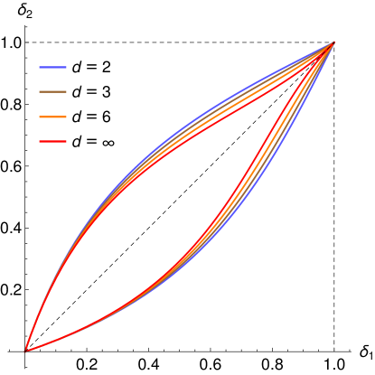
Figure 2: The outer boundary of the region in the $(\delta_{1},\delta_{2})$ plane where the Swap gadget (Algorithm 1) improves the purity of the output compared to both inputs (see Claim 3), for dimensions $d\in\{2,3,6,\infty\}$. As $d$ increases, the region shrinks and converges to the area enclosed by the red curve as $d\to\infty$. For any $d$, the region contains a substantial area surrounding the $\delta_{1}=\delta_{2}$ line, except for the tip at $\delta_{1}=\delta_{2}=1$ which becomes infinitely sharp at $d=\infty$.

Claim 3.

Let $\delta_{1},\delta_{2}\in(0,1)$ and assume (without loss of generality) that $\delta_{2}\geq\delta_{1}$. The output of the Swap gadget (see Algorithm 1) is purer than both inputs $\rho(\delta_{1})$ and $\rho(\delta_{2})$ if and only if

$$\delta_{2}-\delta_{1}<(1-\delta_{1})\frac{2\delta_{1}(d-(d-1)\delta_{1})}{d+2\delta_{1}(d-(d-1)\delta_{1})}.$$ (13)

Proof.

Since we assumed that $\delta_{2}\geq\delta_{1}$, the output is purer than both inputs whenever $\delta_{1}>\delta^{\prime}$ where $\delta^{\prime}$ is given in Claim 2. The denominator of $\delta^{\prime}$ is always positive, so $\delta_{1}>\delta^{\prime}$ is equivalent to

$$\delta_{1}\bigg{\lparen}\Big{\lparen}1+\frac{1}{d}\Big{\rparen}+\Big{\lparen}1-\frac{1}{d}\Big{\rparen}(1-\delta_{1})(1-\delta_{2})\bigg{\rparen}>\frac{\delta_{1}+\delta_{2}}{2}+\frac{\delta_{1}\delta_{2}}{d}.$$ (14)

If we multiply both sides by $2d$ and expand some products, we get

$$2\delta_{1}(d+1)+2\delta_{1}(d-1)(1-\delta_{1}-\delta_{2}+\delta_{1}\delta_{2})>d(\delta_{1}+\delta_{2})+2\delta_{1}\delta_{2},$$ (15)

which can be simplified to an affine function in $\delta_{2}$:

$$\big{\lparen}3d\delta_{1}-2(d-1)\delta_{1}^{2}\big{\rparen}-\big{\lparen}d+2d\delta_{1}-2(d-1)\delta_{1}^{2}\big{\rparen}\delta_{2}>0.$$ (16)

This inequality is equivalent to

$$\frac{3d\delta_{1}-2(d-1)\delta_{1}^{2}}{d+2d\delta_{1}-2(d-1)\delta_{1}^{2}}>\delta_{2},$$ (17)

where the denominator agrees with eq. 13 and is always positive since $\delta_{1}>\delta_{1}^{2}$. If we subtract $\delta_{1}$ from both sides of eq. 17, the numerator becomes

$$\big{\lparen}3d\delta_{1}-2(d-1)\delta_{1}^{2}\big{\rparen}-\big{\lparen}d+2d\delta_{1}-2(d-1)\delta_{1}^{2}\big{\rparen}\delta_{1} =2d\delta_{1}-2(d-1)\delta_{1}^{2}-2d\delta_{1}^{2}+2(d-1)\delta_{1}^{3}$$ (18)

$$=2\delta_{1}(1-\delta_{1})\big{\lparen}d-(d-1)\delta_{1}\big{\rparen},$$

which agrees with eq. 13. ∎

2.4 Swap test on two identical inputs

Note that the right-hand side of eq. 13 is strictly positive for any $\delta_{1}\in(0,1)$. In particular, if $\delta_{1}=\delta_{2}\in(0,1)$ then the left-hand side vanishes while the right-hand side is strictly positive. This means that for identical inputs the output is always purer than both inputs (see also Fig. 2).

Corollary 4.

If $\delta\in(0,1)$ then $\textsc{Swap}(\rho(\delta),\rho(\delta))=\rho(\delta^{\prime})$ where $\delta^{\prime}<\delta$.

This corollary follows immediately from Claim 3 and suggests a simple recursive algorithm that applies the Swap gadget on a pair of identical inputs produced in the previous level of the recursion. Corollary 4 then guarantees that at each subsequent level of recursion, the states become purer. Before we formally state and analyze this recursive procedure, let us first derive the success probability of the swap test on two copies of $\rho(\delta)$, the expected number of copies of $\rho(\delta)$ consumed by the Swap gadget, and the error parameter $\delta^{\prime}$ of the output state $\rho(\delta^{\prime})$.

Recall from eq. 6 that for two identical input states $\rho$, the outcome $a=0$ in the swap test occurs with probability

$$\frac{1}{2}\big{\lparen}1+\operatorname{Tr}(\rho^{2})\big{\rparen}$$ (19)

and, according to eq. 8, the normalized output state is

$$\textsc{Swap}(\rho,\rho)=\frac{\rho+\rho^{2}}{\operatorname{Tr}(\rho+\rho^{2})}.$$ (20)

If we specialize to the case when both input states are $\rho(\delta)$, the success probability of the swap test can be found from eq. 12:

$$p(\delta) :=\frac{1}{2}\bigg{\lparen}\Big{\lparen}1+\frac{1}{d}\Big{\rparen}+\Big{\lparen}1-\frac{1}{d}\Big{\rparen}(1-\delta)^{2}\bigg{\rparen}$$ (21)

$$\>=1-\Big{\lparen}1-\frac{1}{d}\Big{\rparen}\delta+\frac{1}{2}\Big{\lparen}1-\frac{1}{d}\Big{\rparen}\delta^{2}.$$

Accordingly, the expected number of copies of $\rho(\delta)$ consumed by the Swap gadget is

$$\frac{2}{p(\delta)}=\frac{2d}{d-(d-1)\delta+\frac{1}{2}(d-1)\delta^{2}}.$$ (22)

By Claim 2, the output state of the Swap gadget is

$$\textsc{Swap}\big{\lparen}\rho(\delta),\rho(\delta)\big{\rparen}=\rho(\delta^{\prime})\qquad\text{where}\qquad\delta^{\prime}:=\frac{\delta+\delta^{2}/d}{(1+\frac{1}{d})+(1-\frac{1}{d})(1-\delta)^{2}}=\frac{\delta+\delta^{2}/d}{2p(\delta)}.$$ (23)

2.5 Recursive purification based on the swap test

Given access to many copies of $\rho(\delta)$ from eq. 9, with a given value of $\delta\in(0,1)$, our goal is to produce a single copy of $\rho(\epsilon)$, for some desired target parameter $\epsilon\ll\delta$. Since our purification procedure (Algorithm 2) invokes itself recursively, it will be convenient to denote the initial state by $\rho_{0}:=\rho(\delta)$ and the state produced at the $i$th level of the recursion by $\rho_{i}$. We choose the total depth of the recursion later to guarantee a desired level of purity in the final output.

Before stating our algorithm more formally, we emphasize one slightly unusual aspect: even though we fix the total depth of the recursion, the number of calls within each level is not known in advance. This is because each instance of the algorithm calls an instance in the previous recursion level an unknown number of times (as many times as necessary for the Swap gadget to succeed). We analyze the expected number of calls and the total number of input states consumed in Section 3.3.

Algorithm 2 Recursive purification based on the swap test.

This procedure purifies a stream of states $\rho_{0}$ by recursively calling the Swap gadget (Algorithm 1).

1: procedure Purify($n$)

2:      if $n=0$ then If at the bottom level of recursion,

3:          return $\rho_{0}$ request one copy of $\rho_{0}$ from the stream and return it.

4:      else Otherwise call the next level of recursion

5:          return $\textsc{Swap}(\textsc{Purify}(n-1),\textsc{Purify}(n-1))$ until the Swap gadget succeeds.      

Let $\rho_{n}:=\textsc{Purify}(n)$ denote the output of a purification procedure of depth $n$. We can represent this procedure as a full binary tree of height $n$ whose $2^{n}$ leaves correspond to the original input states $\rho_{0}=\rho(\delta)$ and whose root corresponds to the final output state $\rho_{n}$. For any $i\in\{0,\dotsc,n\}$, there are $2^{n-i}$ calls to $\textsc{Purify}(i)$, each producing a copy of $\rho_{i}$ by combining two states from the previous level (or by directly consuming one copy of $\rho_{0}$ when $i=0$). Every time a Swap gadget fails, the recursion is restarted at that level. This triggers a cascade of calls going down all the way to $\textsc{Purify}(0)$, which requests a fresh copy of $\rho_{0}$. Hence, a failure at level $i$ results in at least $2^{i}$ fresh copies of $\rho_{0}$ being requested. The procedure terminates once the outermost Swap gadget succeeds.

According to Corollary 4, the state $\rho_{i}$ is of the form $\rho(\delta_{i})$ for some error parameter $\delta_{i}<\delta_{i-1}$. Denote by $p_{i}$ the probability of success of the Swap gadget in $\textsc{Purify}(i)$ (in other words, $p_{i}$ is the probability of getting outcome $a=0$ when the swap test is applied on two copies of $\rho_{i-1}$). According to eqs. 21 and 23, the parameter $p_{i}$ depends on $\delta_{i}$, while $\delta_{i}$ in turn is found via a recurrence relation:

$$p_{i} =P(\delta_{i-1},d), \delta_{i} =D(\delta_{i-1},d), \delta_{0} =\delta,$$ (24)

where the functions $P,D\colon(0,1)\times[2,\infty)\to(0,1)$ are defined as follows:

$$P(\delta,d) :=1-\Big{\lparen}1-\frac{1}{d}\Big{\rparen}\delta+\frac{1}{2}\Big{\lparen}1-\frac{1}{d}\Big{\rparen}\delta^{2}, D(\delta,d) :=\frac{\delta+\delta^{2}/d}{2P(\delta,d)}.$$ (25)

For any values of the initial purity $\delta_{0}\in(0,1)$ and dimension $d\geq 2$, these recursive relations define a pair of sequences $(p_{1},p_{2},\dotsc)$ and $(\delta_{0},\delta_{1},\dotsc)$. Our goal is to understand the asymptotic scaling of the parameters $p_{i}$ and $\delta_{i}$, and to determine a value $n$ such that $\delta_{n}\leq\epsilon$, for some given $\epsilon>0$.

2.6 Non-recursive stack-based implementation

It is not immediately obvious from the recursive description of $\textsc{Purify}(n)$ in Algorithm 2 that it uses $n+1$ qudits of quantum memory plus one ancilla qubit. Algorithm 3 provides an alternative stack-based implementation of the same procedure that makes this clear.

Algorithm 3 Stack-based implementation of Algorithm 2.

Global variables:

1:$\triangleright$  $\mathrm{qudit}[\cdot]$ – an array of qudits that simulates a stack,

2:$\triangleright$  $\mathrm{purity}[\cdot]$ – an array of integers that store the purity level of each qudit,

3:$\triangleright$  $k$ – an integer that indicates the current position in the stack.

This procedure requests a fresh copy of $\rho_{0}$ from the stream and stores it in the stack.

1: procedure FetchNewCopy

2:      $k$++ Move the stack pointer forward by one.

3:      $\mathrm{qudit}[k]=\rho_{0}$ Fetch a fresh copy of $\rho_{0}$ and store it in the current stack position.

4:      $\mathrm{purity}[k]=0$ Set its purity level to $0$.

Non-recursive implementation of the $\textsc{Purify}(n)$ procedure from Algorithm 2.

1: procedure Purify($n$)

2:      $k=0$ Initially the stack is empty.

3:      $\mathrm{purity}[0]=-1$ Set the purity level of empty stack to a non-existing value.

4:      repeat Repeat until $n$ levels of recursion are reached.

5:          FetchNewCopy Request two fresh copies of $\rho_{0}$

6:          FetchNewCopy and put them in the stack.

7:          repeat Keep merging the two top-most qudits.

8:               Apply the swap test circuit shown in Fig. 1 to $\mathrm{qudit}[k-1]$ and $\mathrm{qudit}[k]$, 9:store the result in $\mathrm{qudit}[k-1]$, and let $a$ be the measurement outcome.

10:               if $a=0$ then If the swap test succeeded,

11:                   $k=k-1$ move the pointer backwards by one (i.e., keep the improved qudit)

12:                   $\mathrm{purity}[k]$++ and increase its purity level by one.

13:               else If the swap test failed,

14:                   $k=k-2$ move the pointer backwards by two (i.e., discard both qudits).               

15:          until $a=1$ or $\mathrm{purity}[k-1]\neq\mathrm{purity}[k]$ Stop if swap test failed or different purities.

16:      until $\mathrm{purity}[1]=n$ Stop when $n$ levels of recursion are reached.

17:      return $\mathrm{qudit}[1]$ Return the only remaining qudit.

3 Analysis of recursive purification

The goal of this section is to analyze the complexity of the recursive purification procedure $\textsc{Purify}(n)$ defined in Algorithm 2. Most of the analysis deals with understanding the recurrence relations in eqs. 24 and 25. First, in Section 3.1 we establish monotonicity of the functions $P$ and $D$ from eq. 25 and the corresponding parameters $p_{i}$ and $\delta_{i}$. In Section 3.2, we analyze the asymptotic scaling of the error parameter $\delta_{i}$. Finally, in Section 3.3, we analyze the expected sample complexity of $\textsc{Purify}(n)$.

3.1 Monotonicity relations

First we prove monotonicity of the functions $P$ and $D$ in eq. 25.

Claim 5.

For any $\delta\in(0,1)$ and $d\geq 2$, the function $P(\delta,d)$ is strictly decreasing in both variables, and the function $D(\delta,d)$ is strictly increasing in both variables.

Proof.

To verify the monotonicity of $P$, note that

$$\frac{\partial P}{\partial\delta} =\Big{\lparen}1-\frac{1}{d}\Big{\rparen}\lparen-1+\delta\rparen<0, \frac{\partial P}{\partial d} =\Big{\lparen}-1+\frac{\delta}{2}\Big{\rparen}\frac{\delta}{d^{2}}<0.$$ (26)

Similarly, the partial derivatives of $D$ are as follows:

$$\frac{\partial D}{\partial\delta} =\frac{1+2\delta/d}{2P(\delta,d)}-\frac{\delta+\delta^{2}/d}{2P(\delta,d)^{2}}\cdot\frac{\partial}{\partial\delta}P(\delta,d)=\frac{(d+2\delta)P(\delta,d)+\delta(d+\delta)(1-1/d)(1-\delta)}{2dP(\delta,d)^{2}}>0,$$ (27)

$$\frac{\partial D}{\partial d} =\frac{-\delta^{2}/d^{2}}{2P(\delta,d)}-\frac{\delta+\delta^{2}/d}{2P(\delta,d)^{2}}\cdot\frac{\partial}{\partial d}P(\delta,d)=\frac{(1-\delta)\delta^{3}}{4d^{2}P(\delta,d)^{2}}>0,$$ (28)

which completes the proof. ∎

Thanks to the recurrence relations in eq. 24, the parameters $p_{i}$ and $\delta_{i}$ inherit the monotonicity of $P$ and $D$ from Claim 5. We denote them by $p_{i}^{(d)}$ and $\delta_{i}^{(d)}$ to explicitly indicate their dependence on $d$. The following claim shows that both parameters are strictly monotonic in the dimension $d$.

Claim 6.

For any $i\geq 1$, the success probability $p_{i}^{(d)}$ is monotonically strictly decreasing in $d$ and the error parameter $\delta_{i}^{(d)}$ is monotonically strictly increasing in $d$, for all integer values of $d\geq 2$.

Proof.

Recall from eq. 24 that $\delta_{0}^{(d)}=\delta=\delta_{0}^{(d+1)}$, irrespective of $d$. Using the recurrence from eq. 24 and the strict monotonicity of $D$ in $d$ from Claim 5,

$$\delta_{1}^{(d)}=D(\delta_{0}^{(d)},d)<D(\delta_{0}^{(d+1)},d+1)=\delta_{1}^{(d+1)}.$$ (29)

Using this as a basis for induction, the strict monotonicity of $D$ in both arguments implies that

$$\delta_{i}^{(d)}=D(\delta_{i-1}^{(d)},d)<D(\delta_{i-1}^{(d+1)},d+1)=\delta_{i}^{(d+1)}$$ (30)

for all $i\geq 1$. We can promote this to a similar inequality for $p_{i}^{(d)}$ using the recurrence from eq. 24. Indeed, this recurrence together with the strict monotonicity of $P$ in both arguments implies that

$$p_{i}^{(d)}=P(\delta_{i-1}^{(d)},d)>P(\delta_{i-1}^{(d+1)},d+1)=p_{i}^{(d+1)}$$ (31)

for all $i\geq 1$. ∎

3.2 Asymptotics of the error parameter

Our goal is to upper bound the error sequence $\delta_{i}^{(d)}$ as a function of $\delta=\delta_{0}^{(d)}$, $d$, and $i$. We also define

$$\delta_{i}^{(\infty)}:=\lim_{d\to\infty}\delta_{i}^{(d)}$$ (32)

for all $i\geq 0$. We can gain some insight and motivate our analysis by examining numerical plots of $\delta_{i}^{(d)}$ as functions of $i$, for some representative values of $d$ and a common $\delta_{0}^{(d)}$ that is very close to $1$, as shown in Fig. 3. To understand the error sequence with a smaller value of $\delta_{0}^{(d)}$, one can simply translate the plot horizontally, starting at a value of $i$ corresponding to the desired initial error.

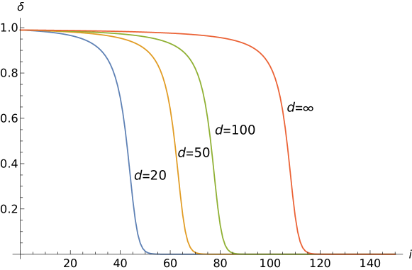
Figure 3: Numerical plots of $\delta_{i}^{(d)}$ for $d=20,50,100$, and of $\delta_{i}^{(\infty)}$, with initial error $\delta_{0}^{(d)}=0.99$.

For each $d$, the sequence $\delta_{i}^{(d)}$ features a slow decline from the initial value $\delta\approx 1$, until it drops to about $0.9$. Then the sequence drops rapidly to about $0.05$ before leveling off and decreasing more slowly. We can establish asymptotic bounds by separately considering the subsequences with $\delta_{i}^{(d)}\geq 1/2$ and $\delta_{i}^{(d)}<1/2$. However, tighter bounds can be obtained by avoiding the threshold $\delta_{i}^{(d)}\approx 1/2$. Thus we consider the subsequences with $\delta_{i}^{(d)}\leq 1/3$, $1/3<\delta_{i}^{(d)}\leq 2/3$, and $2/3<\delta_{i}^{(d)}$. Depending on how small $\delta$ is, we can combine some or all of the above estimates to obtain the number of iterations needed to suppress the error from $\delta$ to $\epsilon$ for arbitrary $d$. We then use these results to bound the sample complexity in Section 3.3. Note that the thresholds $1/3$ and $2/3$ are arbitrary, and can be further optimized as a function of $d$, but we leave such fine tuning to the interested reader.

Our analysis exploits the monotonicity established in Section 3.1: for a common $\delta_{0}^{(d)}$, for all $i,d$, we have $\delta_{i}^{(d)}\leq\delta_{i}^{(d+1)}\leq\delta_{i}^{(\infty)}$, since $D(\delta_{i}^{(d)},d)$ is an increasing function of $d$ and of $\delta_{i}^{(d)}$. We divide our analysis into parts corresponding to the three subsequences:

1. We establish a tight upper bound for $\delta_{i}^{(d)}$ for $\delta_{0}^{(d)}=\delta\leq 1/3$ for all $d\geq 2$. This bound is roughly exponentially decreasing in $i$.

2. For any $d\geq 2$, we show that $3$ to $5$ iterations are enough to reduce $\delta_{i}^{(d)}$ from $2/3$ to $1/3$.

3. For $\delta_{0}^{(d)}>2/3$, and specifically for $\delta_{0}^{(d)}\approx 1$, we are interested in upper bounds on $i^{*}$ so that $\delta_{i^{*}}^{(d)}\approx 2/3$. We further divide this step into three parts.

   1. First, we upper bound $i^{*}$ for $\delta_{0}^{(\infty)}$. Due to Claim 6, the same upper bound holds for other $\delta_{0}^{(d)}$. Combining parts 1, 2, and 33(a), we can upper bound $\delta_{i}^{(d)}$ for all $\delta,i$, and $d$, and in particular, we estimate the number of iterations required (as a function of $\delta=\delta_{0}$ and $\epsilon$) to purify copies of $\rho(\delta)$ into $\rho(\epsilon)$. The number of iterations is a gentle function of $\delta$ and $\epsilon$, and the large-$d$ limit only introduces an additive constant.

   2. Then we tighten the estimate of $i^{*}$ for $\delta_{i}^{(d)}$ with techniques similar to those in part 33(a), but with more complex arithmetic. The resulting estimate applies to all $d\geq 2$ and performs well for small $d(1-\delta)$.

   3. Using a different technique, we obtain a rigorous upper bound for $\delta_{i}^{(d)}$ and $i^{*}$ for all $d\geq 2$. This bound is tight for small to moderate $d(1-\delta)$. For large $d(1-\delta)$, it still has better $\delta$ dependence than the bound in part 33(a) when $1-\delta\ll 1$. We also propose a tight estimate inspired by this bound. This part is also much simpler than part 33(a) and part 33(b), but it only applies to $\delta_{i}^{(d)}\geq 15/16$.

For a rigorous and conceptually simple understanding, one can focus on part 1, part 2 (with $17$ additional iterations to suppress the error from $15/16$ to $2/3$), and part 33(c). The additional estimates and analysis aim to probe the best dependence on $\delta$ and $d$, and to eliminate unnecessary additive constants when bounding the number of iterations. An additive constant in the number of iterations translates to an exponentially large multiplicative constant in the sample complexity (for example, from Section 3.3, $50$ extra iterations lead to at least $2^{50}\approx 10^{15}$ times more samples), so we provide more information for readers who wish to optimize this overhead.

3.2.1 Part 1

If the initial error parameter $\delta_{0}^{(d)}$ is sufficiently small, subsequent values $\delta_{i}^{(d)}$ decrease roughly exponentially in $i$.

Claim 7.

For all $d\geq 2$, if $\delta=\delta_{0}^{(d)}\leq 1/2$, then for all $i\geq 0$,

$$\delta_{i}^{(d)} \leq\frac{\delta}{2^{i}(1-2\delta)+2\delta}.$$ (33)

Proof.

We upper bound $\delta_{i}^{(d)}$ by another sequence $\eta_{i}$ defined as follows:

$$\eta_{0}:=\delta,\quad\eta_{i}:=\frac{\eta_{i-1}}{2-2\eta_{i-1}}\quad{\rm for}~{}i\geq 1.$$ (34)

This recurrence admits an exact solution. Indeed, note that

$$\frac{1}{\eta_{i}}=\frac{2}{\eta_{i-1}}-2,$$ (35)

which yields the following closed-form expression for $\eta_{i}$:

$$\frac{1}{\eta_{i}}=2^{i}\mathopen{}\mathclose{{}\left\lparen\frac{1}{\eta_{0}}-2}\right\rparen+2.$$ (36)

Inverting and substituting $\eta_{0}=\delta$, we find that

$$\eta_{i}=\frac{\delta}{2^{i}(1-2\delta)+2\delta}.$$ (37)

Note that under the assumption $\delta\leq 1/2$ we have $0\leq\eta_{i}\leq 1$ for all $i\geq 0$.

Let us now prove by induction that $\delta_{i}^{(d)}\leq\eta_{i}$ for all $i\geq 0$. Recall from eq. 24 that

$$\delta_{i}^{(d)}=D(\delta_{i-1}^{(d)},d)\leq D(\eta_{i-1},d),$$ (38)

where the inequality follows from the inductive assumption $\delta_{i-1}^{(d)}\leq\eta_{i-1}$ together with Claim 5 and $0\leq\eta_{i-1}\leq 1$. It remains to prove that $D(\eta_{i-1},d)\leq\eta_{i}$. Equivalently, due to eq. 34 we can show that $D(x,d)\leq\frac{x}{2-2x}$ for any $x\in[0,1]$. Recall from eq. 25 that $D(x,d)=\frac{x+x^{2}/d}{2P(x,d)}$, so we need to show that

$$\frac{x+x^{2}/d}{2P(x,d)}\leq\frac{x}{2-2x}.$$ (39)

Since $P(x,d)\geq 0$, we need to show

$$(2-2x)(x+x^{2}/d)\leq 2P(x,d)x.$$ (40)

Substituting $P(x,d)$ from eq. 25 and then expanding, this is equivalent to $0\leq x^{3}(1+1/d)$, which indeed holds for any $x\in[0,1]$. The result then follows from $\delta_{i}^{(d)}\leq\eta_{i}$ and eq. 37. ∎

To suppress the error from $\delta\in(0,1/2)$ to $\epsilon$, since $\eta_{i}<\frac{\delta}{2^{i}(1-2\delta)}$, it suffices to iterate $\log_{2}\frac{\delta}{(1-2\delta)\epsilon}$ times. In particular, for $\delta\leq 1/3$, it suffices to iterate $\log_{2}\frac{1}{\epsilon}$ times.

3.2.2 Part 2

Using monotonicity from Claim 6 and by considering $\delta^{(\infty)}_{i}$, a brute-force calculation shows that $5$ iterations are sufficient to suppress the error from at most $2/3$ to at most $1/3$ for all $d\geq 2$. For smaller values of $d$, as few as $3$ iterations suffice.

3.2.3 Part 33(a)

For $\delta\approx 1$, Fig. 3 suggests that the error suppression is slow until after about $\frac{1}{1-\delta}$ iterations, when the error rapidly drops from $0.9$ to $0.1$. We now study how quickly $\delta_{i}^{(d)}$ can be upper bounded by $2/3$ starting from an arbitrary $\delta_{0}^{(d)}\approx 1$.

We first consider the simpler sequence $\delta_{i}^{(\infty)}$. Note from eq. 25 that

$$\lim_{d\to\infty}D(x,d)=\frac{x}{2-2x+x^{2}},$$ (41)

so $\delta_{i}^{(\infty)}$ obeys the following recurrence:

$$\delta_{0}^{(\infty)}:=\delta,\quad\delta_{i}^{(\infty)}:=\frac{\delta_{i-1}^{(\infty)}}{2-2\delta_{i-1}^{(\infty)}+\delta_{i-1}^{(\infty)2}}\quad{\rm for}~{}i\geq 1.$$ (42)

Because the function $(2-2x+x^{2})^{-1}$ is monotonically increasing for $x\in[0,1]$, and $\delta_{i}^{(\infty)}$ is monotonically decreasing in $i$, the following upper bound holds by induction:

$$\delta_{i}^{(\infty)}\leq\frac{\delta_{i-1}^{(\infty)}}{2-2\delta+\delta^{2}}\leq\frac{\delta}{(2-2\delta+\delta^{2})^{i}}\,.$$ (43)

If $\delta>2/3$ is constant, the above is an exponentially decreasing function in $i$, which may be sufficient for many purposes. However, this bound does not have tight dependence on $\delta$.

We can instead bound $\delta_{i}^{(\infty)}$ by considering two other recurrences, defined as follows. Let $i^{*}$ be the smallest $i$ so that $\delta_{i^{*}+1}^{(\infty)}<2/3$. For $i\in\{0,1,\ldots,i^{*}\}$, let

$$\kappa_{i}^{(\infty)}=1-\delta_{i}^{(\infty)},$$ (44)

so that

$$\kappa_{0}^{(\infty)}=1-\delta,\quad\kappa_{i}^{(\infty)}=1-\delta_{i}^{(\infty)}=1-\frac{\delta_{i-1}^{(\infty)}}{2-2\delta_{i-1}^{(\infty)}+\delta_{i-1}^{(\infty)2}}=\frac{\kappa_{i-1}^{(\infty)}+\kappa_{i-1}^{(\infty)2}}{1+\kappa_{i-1}^{(\infty)2}}.$$ (45)

Furthermore, for $i\in\{0,1,\ldots,i^{*}\}$, define an inverse recurrence for $\kappa_{i}^{(\infty)}$ as

$$\mu_{0}^{(\infty)}=\kappa_{i^{*}}^{(\infty)},\quad\mu_{i}^{(\infty)}=h^{(\infty)}(\mu_{i-1}^{(\infty)})$$ (46)

where $h^{(\infty)}(y)$ is the inverse of $y=g^{(\infty)}(x)=\frac{x+x^{2}}{1+x^{2}}$ (which is well-defined for all $x\in[0,1]$), so indeed, $\mu_{i}^{(\infty)}=\kappa_{i^{*}-i}^{(\infty)}$.

Our main idea is as follows. We can estimate $\mu_{i}^{(\infty)}$ as a function of $i$. Furthermore, if we prove an upper bound $\upsilon$ for $\mu_{i}^{(\infty)}$, we have a lower bound $1-\upsilon$ for $\delta_{i^{*}-i}^{(\infty)}$, which means that $i+1$ iterations are sufficient to reduce $\delta_{i^{*}-i}^{(\infty)}$ from at least $1-\upsilon$ to $\delta_{i^{*}+1}^{(\infty)}<1/3$. In particular, if $n$ satisfies $\mu_{n}^{(\infty)}\leq 1-\delta$, then $n+1$ iterations are sufficient to reduce the initial error $\delta_{0}^{(\infty)}=\delta$ to $\delta_{n+1}^{(\infty)}<2/3$ so $i^{*}<n$. Overall, this analysis suggests that if $\mu_{0}^{(\infty)}\leq 1/3$, then for all $i$,

$$\mu_{i}^{(\infty)}<\frac{1}{i}+\frac{2.5\ln i}{i^{2}}.$$ (47)

To show this, we first find a Taylor series expansion for $h^{(\infty)}(y)$ by inverting $y=\frac{x+x^{2}}{1+x^{2}}$ for small positive $x$ and $y$. We have $(1-y)x^{2}+x-y=0$, so, using the quadratic formula,

$$x=\frac{-1+\sqrt{1+4y(1-y)}}{2(1-y)}.$$ (48)

Note that we only keep the solution corresponding to the case of interest, $0<x,y<1/3$ (because $1/3>\mu_{0}^{(\infty)}$ and $\mu_{i}^{(\infty)}$ is decreasing with $i$ while remaining positive). Since $4y(1-y)\leq 8/9$ for $y<1/3$, we can apply the formula $\sqrt{1+a}=1+\frac{a}{2}-\frac{a^{2}}{8}+\frac{a^{3}}{16}+\cdots$ , together with the geometric series expansion for the denominator, to obtain

$$x=y-y^{2}+3y^{3}+o(y^{3})=h^{(\infty)}(y).$$ (49)

(Note that for $y\approx 1/2$, we have $4y(1-y)\approx 1$, so the above expansion is invalid. This is why we use part 2 to avoid that parameter range.)

Next we invoke a theorem from [Ste96] (case 2), which says that

$$\mu_{i}^{(\infty)}=\frac{1}{i}+\frac{2\ln i}{i^{2}}+o\mathopen{}\mathclose{{}\left(\frac{\ln i}{i^{2}}}\right).$$ (50)

To be self-contained, and to motivate the derivation in part 33(b), we include the derivation from [Ste96] as follows. Since

$$\mu_{i}^{(\infty)}=h^{(\infty)}(\mu_{i-1}^{(\infty)})=\mu_{i-1}^{(\infty)}-\mu_{i-1}^{(\infty)2}+3\mu_{i-1}^{(\infty)3}+o(\mu_{i-1}^{(\infty)3})$$ (51)

and $(1-x)^{-1}=1+x+x^{2}+O(x^{3})$ for small $x$, we have

$$\frac{1}{\mu_{i}^{(\infty)}} =\frac{1}{\mu_{i-1}^{(\infty)}}\times\frac{1}{1-\mu_{i-1}^{(\infty)}+3\mu_{i-1}^{(\infty)2}+o(\mu_{i-1}^{(\infty)2})}$$ (52)

$$\approx\frac{1}{\mu_{i-1}^{(\infty)}}\times\mathopen{}\mathclose{{}\left(1+\mu_{i-1}^{(\infty)}-3\mu_{i-1}^{(\infty)2}+\mu_{i-1}^{(\infty)2}+o(\mu_{i-1}^{(\infty)2})}\right)$$ (53)

$$\approx\frac{1}{\mu_{i-1}^{(\infty)}}+1-2\mu_{i-1}^{(\infty)}+o\mathopen{}\mathclose{{}\left(\mu_{i-1}^{(\infty)2}}\right)$$ (54)

$$\approx\frac{1}{\mu_{0}^{(\infty)}}+i-2\sum_{j=0}^{i-1}\mu_{j}^{(\infty)}+\sum_{j=0}^{i-1}o\mathopen{}\mathclose{{}\left(\mu_{j}^{(\infty)2}}\right).$$ (55)

The right-hand side is dominated by $i$, so $\mu_{i}^{(\infty)}\approx\frac{1}{i}$. Substituting this into the sum $\sum_{j=0}^{i-1}\mu_{j}^{(\infty)}$ above, and using Euler’s formula $1+\frac{1}{2}+\cdots+\frac{1}{i}\approx\ln i$, we have

$$\frac{1}{\mu_{i}^{(\infty)}}\approx\frac{1}{\mu_{0}^{(\infty)}}+i-2\ln i\approx i-2\ln i$$ (56)

and therefore

$$\mu_{i}^{(\infty)}\approx\frac{1}{i-2\ln i}\approx\frac{1}{i}+\frac{2\ln i}{i^{2}}+o\mathopen{}\mathclose{{}\left(\frac{\ln i}{i^{2}}}\right).$$ (57)

While the above estimate involves several approximations, and $\mu_{i}^{(\infty)}$ is not so small for small $i$, the resulting estimate is surprisingly tight. Indeed, we can numerically confirm the upper bound

$$\mu_{i}^{(\infty)}<\frac{1}{i}+\frac{2.5\ln i}{i^{2}}$$ (58)

by generating an upper bound on the sequence using the worst-case initial value $\mu_{0}^{(\infty)}=1/3$.

Using the above analysis, we can infer that for any $\delta\in(2/3,1)$, if

$$n\approx\frac{1}{1-\delta}\mathopen{}\mathclose{{}\left(1+2.5(1-\delta)\ln\mathopen{}\mathclose{{}\left(\frac{1}{1-\delta}}\right)}\right)=\frac{1}{1-\delta}+2.5\ln\mathopen{}\mathclose{{}\left(\frac{1}{1-\delta}}\right),$$ (59)

then $\mu_{n}^{(\infty)}\leq 1-\delta$. Thus we conclude that for some $i^{*}$ that is at most the value of $n$ in eq. 59, $\delta_{i^{*}+1}^{(\infty)}<2/3$.

As a comparison, if we use the rough upper bound for $\delta_{i}^{(\infty)}$ in eq. 43, we conclude that the upper bound is less than $2/3$ after $n$ iterations if

$$n\geq\mathopen{}\mathclose{{}\left\lceil\frac{\ln(3\delta/2)}{\ln(2-2\delta+\delta^{2})}}\right\rceil.$$ (60)

When $1-\delta\ll 1$, $\ln(2-2\delta+\delta^{2})=\ln(1+(1-\delta)^{2})\approx(1-\delta)^{2}$, so the upper bound on the number of iterations is roughly

$$n\geq\mathopen{}\mathclose{{}\left\lceil\frac{\ln(3\delta/2)}{(1-\delta)^{2}}}\right\rceil,$$ (61)

with quadratically worse dependence on $\frac{1}{1-\delta}$.

Combining parts 1, 2, and 33(a), we have established the following estimate. For all $d\geq 2$, $\delta>2/3$, and $\epsilon$ with $\delta>\epsilon>0$, the error can be reduced from $\delta$ to $\epsilon$ with at most

$$\log_{2}\frac{1}{\epsilon}+5+\frac{1}{1-\delta}+2.5\ln\mathopen{}\mathclose{{}\left(\frac{1}{1-\delta}}\right)$$ (62)

iterations.

3.2.4 Part 33(b)

We now provide a more refined analysis of $\delta_{i}^{(d)}$ for finite $d$ and for $\delta\approx 1$. In this part, we use a method similar to part 33(a), with more complex arithmetic. A more relaxed bound with a simpler derivation is presented in part 33(c).

The goal is to upper bound the recurrence

$$\delta_{0}^{(d)} =\delta,\quad\delta_{i}^{(d)}=D(\delta_{i-1}^{(d)},d)=\frac{\delta_{i-1}^{(d)}+\frac{1}{d}\;\delta_{i-1}^{(d)2}}{2\mathopen{}\mathclose{{}\left(1-\Big{\lparen}1-\frac{1}{d}\Big{\rparen}\delta_{i-1}^{(d)}+\frac{1}{2}\Big{\lparen}1-\frac{1}{d}\Big{\rparen}\delta_{i-1}^{(d)2}}\right)}$$ (63)

stated in eqs. 24 and 25. As in part 33(a), let $i^{*}$ be the smallest integer so that $\delta_{i^{*}+1}^{(d)}<2/3$. For $i\in\{0,1,\ldots,i^{*}\}$, let

$$\kappa_{i}^{(d)}=1-\delta_{i}^{(d)},$$ (64)

which implies

$$\kappa_{0}^{(d)}=1-\delta,\quad\kappa_{i}^{(d)}=1-\delta_{i}^{(d)}=\frac{\mathopen{}\mathclose{{}\left(1+\frac{2}{d}}\right)\kappa_{i-1}^{(d)}+\mathopen{}\mathclose{{}\left(1-\frac{2}{d}}\right)\kappa_{i-1}^{(d)2}}{\mathopen{}\mathclose{{}\left(1+\frac{1}{d}}\right)+\mathopen{}\mathclose{{}\left(1-\frac{1}{d}}\right)\kappa_{i-1}^{(d)2}},$$ (65)

where we have first expressed $\delta_{i}^{(d)}$ in terms of $\delta_{i-1}^{(d)}$ and then substituted $\delta_{i-1}^{(d)}=1-\kappa_{i-1}^{(d)}$ to obtain the recurrence. For $i\in\{0,1,\ldots,i^{*}\}$, by inverting $y=\frac{(1+\frac{2}{d})x+(1-\frac{2}{d})x^{2}}{(1+\frac{1}{d})+(1-\frac{1}{d})x^{2}}$, define an inverse recurrence for $\kappa_{i}^{(d)}$ by applying the quadratic formula to solve for $x$ in terms of $y$, giving

$$x=\frac{-\mathopen{}\mathclose{{}\left(1+\frac{2}{d}}\right)\pm\sqrt{\mathopen{}\mathclose{{}\left(1+\frac{2}{d}}\right)^{2}+4\Bigl{(}\mathopen{}\mathclose{{}\left(1-\frac{2}{d}}\right)-\mathopen{}\mathclose{{}\left(1-\frac{1}{d}}\right)y\Bigr{)}\mathopen{}\mathclose{{}\left(1+\frac{1}{d}}\right)y}}{2\Bigl{(}\mathopen{}\mathclose{{}\left(1-\frac{2}{d}}\right)-\mathopen{}\mathclose{{}\left(1-\frac{1}{d}}\right)y\Bigr{)}}.$$ (66)

In the above, we have assumed $\mathopen{}\mathclose{{}\left(1-\frac{2}{d}}\right)-\mathopen{}\mathclose{{}\left(1-\frac{1}{d}}\right)y>0$. For $d\geq 3$ and $0<y<1/3$ (since $y$ represents $\mu_{i}^{(d)}$, which decreases from $\mu_{0}^{(d)}<1/3$ to $\mu_{i^{*}}^{(d)}\approx 1-\delta$), this assumption holds. Also, only the “$+$” solution gives rise to a valid recurrence because the “$-$” solution is negative. For $d=2$, the above expression still represents the roots. The “$-$” solution is larger than $1$, so again, only the “$+$” solution is valid.

To proceed, we apply a Taylor series expansion to the square root and if $d\geq 3$, we apply the geometric series expansion to the denominator. Provided $y<1/3$, the expansions provide good estimates. We obtain the following expansion:

$$x =a\mathopen{}\mathclose{{}\left(y-by^{2}+cy^{3}+O(y^{4})}\right)=h^{(d)}(y),~{}\text{where}$$ (67)

$$a =\frac{1+\frac{1}{d}}{1+\frac{2}{d}}$$ (68)

$$b =\frac{\mathopen{}\mathclose{{}\left(1+\frac{1}{d}}\right)\mathopen{}\mathclose{{}\left(1-\frac{2}{d}}\right)}{\mathopen{}\mathclose{{}\left(1+\frac{2}{d}}\right)^{2}}$$ (69)

$$c =\frac{1+\frac{1}{d}}{\mathopen{}\mathclose{{}\left(1+\frac{2}{d}}\right)^{2}}\times\mathopen{}\mathclose{{}\left(\mathopen{}\mathclose{{}\left(1-\frac{1}{d}}\right)+2\frac{\mathopen{}\mathclose{{}\left(1+\frac{1}{d}}\right)\mathopen{}\mathclose{{}\left(1-\frac{2}{d}}\right)^{2}}{\mathopen{}\mathclose{{}\left(1+\frac{2}{d}}\right)^{2}}}\right).$$ (70)

Therefore,

$$\mu_{i}^{(d)}=h^{(d)}(\mu_{i-1}^{(d)})=a\mathopen{}\mathclose{{}\left(\mu_{i-1}^{(d)}-b\mu_{i-1}^{(d)2}+c\mu_{i-1}^{(d)3}+O(\mu_{i-1}^{(d)4})}\right).$$ (71)

Similarly to part 33(a), we obtain

$$\frac{1}{\mu_{i}^{(d)}} =\frac{1}{a}\times\frac{1}{\mu_{i-1}^{(d)}}\times\frac{1}{1-b\mu_{i-1}^{(d)}+c\mu_{i-1}^{(d)2}+O(\mu_{i-1}^{(d)3})}$$ (72)

$$\approx\frac{1}{a}\times\frac{1}{\mu_{i-1}^{(d)}}\times\mathopen{}\mathclose{{}\left(1+b\mu_{i-1}^{(d)}+(b^{2}-c)\mu_{i-1}^{(d)2}+O(\mu_{i-1}^{(d)3})}\right)$$ (73)

$$\approx\frac{1}{a}\times\mathopen{}\mathclose{{}\left(\frac{1}{\mu_{i-1}^{(d)}}+b+(b^{2}-c)\mu_{i-1}^{(d)}}\right)$$ (74)

$$\approx\frac{1}{a}\times\mathopen{}\mathclose{{}\left(\frac{1}{a}\times\mathopen{}\mathclose{{}\left(\frac{1}{\mu_{i-2}^{(d)}}+b+(b^{2}-c)\mu_{i-2}^{(d)}}\right)+b+(b^{2}-c)\mu_{i-1}^{(d)}}\right)$$ (75)

$$=\frac{1}{a^{i}}\frac{1}{\mu_{0}^{(d)}}+b\mathopen{}\mathclose{{}\left(\frac{1}{a^{i}}+\cdots+\frac{1}{a}}\right)+(b^{2}-c)\sum_{j=1}^{i}\frac{1}{a^{j}}\mu_{i-j}^{(d)}$$ (76)

$$=\frac{1}{a^{i}}\mathopen{}\mathclose{{}\left(\frac{1}{\mu_{0}^{(d)}}+b\mathopen{}\mathclose{{}\left(\frac{1-a^{i}}{1-a}}\right)}\right)+(b^{2}-c)\sum_{j=1}^{i}\frac{1}{a^{j}}\mu_{i-j}^{(d)}.$$ (77)

For $a^{i}\ll 1$, the first term above suggests an ansatz $\mu_{i}^{(d)}\approx a^{i}t$ for some $t$. Substituting this ansatz into the last term, we obtain

$$\frac{1}{\mu_{i}^{(d)}} \approx\frac{1}{a^{i}}\mathopen{}\mathclose{{}\left(\frac{1}{\mu_{0}^{(d)}}+b\mathopen{}\mathclose{{}\left(\frac{1-a^{i}}{1-a}}\right)}\right)+(b^{2}-c)\sum_{j=1}^{i}ta^{i-2j}$$ (78)

$$=\frac{1}{a^{i}}\mathopen{}\mathclose{{}\left(\frac{1}{\mu_{0}^{(d)}}+b\mathopen{}\mathclose{{}\left(\frac{1-a^{i}}{1-a}}\right)}\right)+(b^{2}-c)ta^{-i}\frac{1-a^{2i}}{1-a^{2}}$$ (79)

$$=\frac{1}{a^{i}}\mathopen{}\mathclose{{}\left(\frac{1}{\mu_{0}^{(d)}}+b\mathopen{}\mathclose{{}\left(\frac{1-a^{i}}{1-a}}\right)+(b^{2}-c)t\frac{1-a^{2i}}{1-a^{2}}}\right).$$ (80)

If there is a positive solution for $t$, we can conclude that $\mu_{i}^{(d)}\approx ta^{i}=t\mathopen{}\mathclose{{}\left(\frac{d+1}{d+2}}\right)^{i}$. Substituting this into the left-hand side, we obtain the equation

$$\frac{1}{t}=\frac{1}{\mu_{0}^{(d)}}+b\mathopen{}\mathclose{{}\left(\frac{1-a^{i}}{1-a}}\right)+(b^{2}-c)t\frac{1-a^{2i}}{1-a^{2}}.$$ (81)

For large $i$, $a^{i}\ll 1$, so

$$1-a^{2}=\frac{t(1-a^{2})}{\mu_{0}^{(d)}}+tb(1+a)+(b^{2}-c)t^{2}.$$ (82)

Rearranging the terms,

$$1-a^{2}-t\mathopen{}\mathclose{{}\left(\frac{(1-a^{2})}{\mu_{0}^{(d)}}+b(1+a)}\right)+(c-b^{2})t^{2}=0.$$ (83)

Let $\tilde{c}=1-a^{2}$, $\tilde{b}=\frac{(1-a^{2})}{\mu_{0}^{(d)}}+b(1+a)$, and $\tilde{a}=c-b^{2}$ so we are solving $0=\tilde{c}-\tilde{b}t+\tilde{a}t^{2}$. The roots are determined by the quadratic formula, which gives

$$t=\frac{\tilde{b}}{2\tilde{a}}\mathopen{}\mathclose{{}\left(1\pm\sqrt{1-\frac{\tilde{c}/\tilde{a}}{(\tilde{b}/(2\tilde{a}))^{2}}}}\right).$$ (84)

Both roots are positive, but only the “$-$” solution gives a tight estimate for $\mu_{i}^{(d)}\approx ta^{i}$ for the following reason. In eq. 73, the $(b^{2}-c)\mu_{i-1}^{(d)2}$ term is a higher-order term that can be dropped when $\mu_{i-1}^{(d)}\ll 1$, and doing so gives the root $\tilde{c}/\tilde{b}$. Thus the corresponding $(c-b^{2})t^{2}$ term in eq. 83 can be viewed as a perturbation, leading to a solution close to $\tilde{c}/\tilde{b}$, which is the “$-$” solution above. Let $t^{*}$ be this solution.

We examine our estimates of $\mu_{i}^{(d)}$ and $i^{*}$ for representative cases of $d$, with a fixed $\delta=0.99$. For $d=2$, numerically evaluating $\delta_{i}^{(2)}$ gives $i^{*}=12,\delta_{i^{*}}^{(2)}\approx 0.697$, and $\mu_{0}^{(2)}\approx 0.303$. We have $a=3/4$, $b=0$ (this is exceptional for $d=2$), $c\approx 0.1875$, $\tilde{a}\approx 0.18750$, $\tilde{b}\approx 1.4441$, $\tilde{c}\approx 0.4375$, and $t^{*}\approx 0.316$, which gives a numerically very tight bound for all $\mu_{i}^{(2)}$. In particular, $t^{*}a^{i^{*}}/\mu_{i^{*}}^{(2)}\approx 1.0007$, so the correct $i^{*}$ is obtained from the estimate. This $i^{*}$ is $100$ iterations fewer than the $d=\infty$ upper bound.

For the small value $d=5$, numerically evaluating $\delta_{i}^{(5)}$ gives $i^{*}=19,\delta_{i^{*}}^{(3)}\approx 0.71$, and $\mu_{0}^{(2)}\approx 0.329$. We have $a\approx 0.857$, $b\approx 0.367$, $c\approx 0.760$, $\tilde{a}\approx 0.625$, $\tilde{b}\approx 1.598$, $\tilde{c}\approx 0.265$, and $t^{*}\approx 0.1785$. Here, the estimate $t^{*}a^{i}$ for $\mu_{i}^{(5)}$ is poor for smaller values of $i$, but is within $5\%$ for $i$ closer to $i^{*}$, which is the regime of interest. In particular, the estimate still gives the correct $i^{*}$, and this estimate is 93 iterations better than the $d=\infty$ upper bound.

For $d=20$, corresponding to the first (blue) curve in Fig. 3, numerically evaluating $\delta_{i}^{(20)}$ gives $i^{*}=40,\delta_{i^{*}}^{(20)}\approx 0.691$, and $\mu_{0}^{(d)}\approx 0.309$. Meanwhile, $a\approx 0.955$, $b\approx 0.781$, $c\approx 0.20443$, $\tilde{a}=1.434$, $\tilde{b}=1.814$, $\tilde{c}=0.089$, $t^{*}\approx 0.051$, and the estimated $i^{*}$ is $36$. The main inaccuracy is due to dropping $a^{i}$, which is between 0.16 and 0.18 for $i\approx i^{*}$.

As $d$ becomes large and $a\rightarrow 1$, this estimate becomes less accurate. Our estimate works best for very small $1-\delta$, giving

$$i^{*}\approx\frac{\ln\frac{t^{*}}{1-\delta}}{\ln\frac{1}{a}}=\frac{\ln\frac{t^{*}}{1-\delta}}{\ln\frac{d+2}{d+1}}$$ (85)

iterations. Expanding $\ln\frac{d+2}{d+1}\approx\frac{1}{d}$, if $d\ll\frac{1}{1-\delta}$, then part 33(b) provides a better bound than the bound $\frac{1}{1-\delta}$ for $d\ll\frac{1}{1-\delta}$ from part 33(a).

3.2.5 Part 33(c)

The above estimates do not provide a strict upper bound on the sequence $\delta^{(d)}_{i}$ or the value of $i^{*}$. In this part, we return to a technique similar to that in part 1 to obtain a strict upper bound for any $d$ and $\delta$. In particular, this bound performs well even for large $d(1-\delta)$, and is tight for dimensions up to the hundreds. The analysis is simpler than part 33(b), but requires $\delta^{(d)}_{i}>15/16$. Numerically, one can confirm that $17$ more steps are enough to reduce the error from $15/16$ to $2/3$, after which results from parts 2 and 1 become applicable.

Recall from eq. 65 in part 33(b) that

$$\kappa_{0}^{(d)}=1-\delta,\quad\kappa_{i}^{(d)}=1-\delta_{i}^{(d)}=K(\kappa_{i-1}^{(d)},d)$$ (86)

where

$$K(x,d)=\frac{\mathopen{}\mathclose{{}\left(1+\frac{2}{d}}\right)x+\mathopen{}\mathclose{{}\left(1-\frac{2}{d}}\right)x^{2}}{\mathopen{}\mathclose{{}\left(1+\frac{1}{d}}\right)+\mathopen{}\mathclose{{}\left(1-\frac{1}{d}}\right)x^{2}}.$$ (87)

To upper bound $\delta_{i}^{(d)}$, we want to lower bound $\kappa_{i}^{(d)}$. We can do so using another sequence $\bar{\kappa}_{i}^{(d)}$ defined as

$$\bar{\kappa}_{0}^{(d)}=\kappa_{0}^{(d)},\quad\bar{\kappa}_{i}^{(d)}=\bar{K}(\bar{\kappa}_{i-1}^{(d)},d)$$ (88)

where

$$\bar{K}(x,d)=\frac{\alpha x}{1-\beta x}$$ (89)

with

$$\alpha=\frac{1+\frac{2}{d}}{1+\frac{1}{d}}=\frac{d+2}{d+1},\quad\beta=\frac{d-2}{d+2}-\frac{1}{8},$$ (90)

so that

$$0<\bar{K}(x,d)<K(x,d)$$ (91)

for all $d\geq 2$ and for $0<x<1/16$. (The choices for $\alpha,\beta$ are motivated by appropriate expansions of $K(x,d)$ and $\bar{K}(x,d)$, and the inequality (91) can be verified analytically.)

Define $j^{*}$ to be the smallest $i$ such that $\bar{\kappa}_{i}^{(d)}\geq 1/16$. Note that $j^{*}\geq 1$ since $\bar{\kappa}_{0}^{(d)}<1/16$. Using inequality (91), the monotonicity of $K,\bar{K}$, and induction on $i$, we can show that $\kappa_{i}^{(d)}>\bar{\kappa}_{i}^{(d)}$ for $1\leq i\leq j^{*}$. In particular,

$$\kappa_{j^{*}}^{(d)}>\bar{\kappa}_{j^{*}}^{(d)}\geq 1/16.$$ (92)

Furthermore, eq. 89 implies that the recurrence $\bar{\kappa}_{i}^{(d)}$ satisfies the relation

$$\frac{\bar{\kappa}_{i}^{(d)}}{\bar{\kappa}_{i}^{(d)}+\frac{\alpha-1}{\beta}}=\frac{\alpha\bar{\kappa}_{i-1}^{(d)}}{\alpha\bar{\kappa}_{i-1}^{(d)}+(1-\beta\bar{\kappa}_{i-1}^{(d)})\frac{\alpha-1}{\beta}}=\frac{\alpha\bar{\kappa}_{i-1}^{(d)}}{\bar{\kappa}_{i-1}^{(d)}+\frac{\alpha-1}{\beta}}=\cdots=\alpha^{i}\frac{\bar{\kappa}_{0}^{(d)}}{\bar{\kappa}_{0}^{(d)}+\frac{\alpha-1}{\beta}}\,.$$ (93)

We can obtain a closed-form expression for $\bar{\kappa}_{i}^{(d)}$, but that is not needed for an upper bound on $j^{*}$. For $d\geq 3$, $\frac{\alpha-1}{\beta}>0$, so $\frac{x}{x+\frac{\alpha-1}{\beta}}$ is strictly increasing with $x$. Therefore, $\bar{\kappa}_{i}^{(d)}>1/16$ if and only if

$$\frac{\bar{\kappa}_{i}^{(d)}}{\bar{\kappa}_{i}^{(d)}+\frac{\alpha-1}{\beta}}>\frac{\frac{1}{16}}{\frac{1}{16}+\frac{\alpha-1}{\beta}}.$$ (94)

Together with eq. 93, $\bar{\kappa}_{i}^{(d)}>1/16$ if and only if

$$\alpha^{i}\frac{\bar{\kappa}_{0}^{(d)}}{\bar{\kappa}_{0}^{(d)}+\frac{\alpha-1}{\beta}}>\frac{\frac{1}{16}}{\frac{1}{16}+\frac{\alpha-1}{\beta}}$$ (95)

or, solving the inequality using the continuous extension for $i$, applying the ceiling to obtain integer values of $i$, and simplifying the fractions, we obtain

$$i\geq{\mathchoice{\ooalign{\clipbox{0pt {} 0pt 0pt}{\hbox{\set@color$\displaystyle\mathopen{}\mathclose{{}\left\lceil\rule{0.0pt}{19.39772pt}}\right.$}}\cr\raisebox{-2.5pt}{\clipbox{0pt 0pt 0pt {}}{\hbox{\set@color$\displaystyle\mathopen{}\mathclose{{}\left\lceil\rule{0.0pt}{19.39772pt}}\right.$}}}\cr}\hbox{\set@color$\displaystyle\frac{\ln\frac{1+\frac{\alpha-1}{\beta\bar{\kappa}_{0}^{(d)}}}{1+\frac{\alpha-1}{\beta}16}}{\ln\alpha}$}\ooalign{\clipbox{0pt {} 0pt 0pt}{\hbox{\set@color$\displaystyle\mathopen{}\mathclose{{}\left.\rule{0.0pt}{19.39772pt}}\right\rceil$}}\cr\raisebox{-2.5pt}{\clipbox{0pt 0pt 0pt {}}{\hbox{\set@color$\displaystyle\mathopen{}\mathclose{{}\left.\rule{0.0pt}{19.39772pt}}\right\rceil$}}}\cr}}{\ooalign{\clipbox{0pt {} 0pt 0pt}{\hbox{\set@color$\textstyle\mathopen{}\mathclose{{}\left\lceil\rule{0.0pt}{18.56439pt}}\right.$}}\cr\raisebox{-2.5pt}{\clipbox{0pt 0pt 0pt {}}{\hbox{\set@color$\textstyle\mathopen{}\mathclose{{}\left\lceil\rule{0.0pt}{18.56439pt}}\right.$}}}\cr}\hbox{\set@color$\textstyle\frac{\ln\frac{1+\frac{\alpha-1}{\beta\bar{\kappa}_{0}^{(d)}}}{1+\frac{\alpha-1}{\beta}16}}{\ln\alpha}$}\ooalign{\clipbox{0pt {} 0pt 0pt}{\hbox{\set@color$\textstyle\mathopen{}\mathclose{{}\left.\rule{0.0pt}{18.56439pt}}\right\rceil$}}\cr\raisebox{-2.5pt}{\clipbox{0pt 0pt 0pt {}}{\hbox{\set@color$\textstyle\mathopen{}\mathclose{{}\left.\rule{0.0pt}{18.56439pt}}\right\rceil$}}}\cr}}{\ooalign{\clipbox{0pt {} 0pt 0pt}{\hbox{\set@color$\scriptstyle\mathopen{}\mathclose{{}\left\lceil\rule{0.0pt}{18.00883pt}}\right.$}}\cr\raisebox{-2.5pt}{\clipbox{0pt 0pt 0pt {}}{\hbox{\set@color$\scriptstyle\mathopen{}\mathclose{{}\left\lceil\rule{0.0pt}{18.00883pt}}\right.$}}}\cr}\hbox{\set@color$\scriptstyle\frac{\ln\frac{1+\frac{\alpha-1}{\beta\bar{\kappa}_{0}^{(d)}}}{1+\frac{\alpha-1}{\beta}16}}{\ln\alpha}$}\ooalign{\clipbox{0pt {} 0pt 0pt}{\hbox{\set@color$\scriptstyle\mathopen{}\mathclose{{}\left.\rule{0.0pt}{18.00883pt}}\right\rceil$}}\cr\raisebox{-2.5pt}{\clipbox{0pt 0pt 0pt {}}{\hbox{\set@color$\scriptstyle\mathopen{}\mathclose{{}\left.\rule{0.0pt}{18.00883pt}}\right\rceil$}}}\cr}}{\ooalign{\clipbox{0pt {} 0pt 0pt}{\hbox{\set@color$\scriptscriptstyle\mathopen{}\mathclose{{}\left\lceil\rule{0.0pt}{18.00883pt}}\right.$}}\cr\raisebox{-2.5pt}{\clipbox{0pt 0pt 0pt {}}{\hbox{\set@color$\scriptscriptstyle\mathopen{}\mathclose{{}\left\lceil\rule{0.0pt}{18.00883pt}}\right.$}}}\cr}\hbox{\set@color$\scriptscriptstyle\frac{\ln\frac{1+\frac{\alpha-1}{\beta\bar{\kappa}_{0}^{(d)}}}{1+\frac{\alpha-1}{\beta}16}}{\ln\alpha}$}\ooalign{\clipbox{0pt {} 0pt 0pt}{\hbox{\set@color$\scriptscriptstyle\mathopen{}\mathclose{{}\left.\rule{0.0pt}{18.00883pt}}\right\rceil$}}\cr\raisebox{-2.5pt}{\clipbox{0pt 0pt 0pt {}}{\hbox{\set@color$\scriptscriptstyle\mathopen{}\mathclose{{}\left.\rule{0.0pt}{18.00883pt}}\right\rceil$}}}\cr}}}={\mathchoice{\ooalign{\clipbox{0pt {} 0pt 0pt}{\hbox{\set@color$\displaystyle\mathopen{}\mathclose{{}\left\lceil\rule{0.0pt}{17.51106pt}}\right.$}}\cr\raisebox{-2.5pt}{\clipbox{0pt 0pt 0pt {}}{\hbox{\set@color$\displaystyle\mathopen{}\mathclose{{}\left\lceil\rule{0.0pt}{17.51106pt}}\right.$}}}\cr}\hbox{\set@color$\displaystyle\frac{\ln\frac{1+\frac{1}{(d+1)\beta(1-\delta)}}{1+\frac{16}{(d+1)\beta}}}{\ln\frac{d+2}{d+1}}$}\ooalign{\clipbox{0pt {} 0pt 0pt}{\hbox{\set@color$\displaystyle\mathopen{}\mathclose{{}\left.\rule{0.0pt}{17.51106pt}}\right\rceil$}}\cr\raisebox{-2.5pt}{\clipbox{0pt 0pt 0pt {}}{\hbox{\set@color$\displaystyle\mathopen{}\mathclose{{}\left.\rule{0.0pt}{17.51106pt}}\right\rceil$}}}\cr}}{\ooalign{\clipbox{0pt {} 0pt 0pt}{\hbox{\set@color$\textstyle\mathopen{}\mathclose{{}\left\lceil\rule{0.0pt}{16.26662pt}}\right.$}}\cr\raisebox{-2.5pt}{\clipbox{0pt 0pt 0pt {}}{\hbox{\set@color$\textstyle\mathopen{}\mathclose{{}\left\lceil\rule{0.0pt}{16.26662pt}}\right.$}}}\cr}\hbox{\set@color$\textstyle\frac{\ln\frac{1+\frac{1}{(d+1)\beta(1-\delta)}}{1+\frac{16}{(d+1)\beta}}}{\ln\frac{d+2}{d+1}}$}\ooalign{\clipbox{0pt {} 0pt 0pt}{\hbox{\set@color$\textstyle\mathopen{}\mathclose{{}\left.\rule{0.0pt}{16.26662pt}}\right\rceil$}}\cr\raisebox{-2.5pt}{\clipbox{0pt 0pt 0pt {}}{\hbox{\set@color$\textstyle\mathopen{}\mathclose{{}\left.\rule{0.0pt}{16.26662pt}}\right\rceil$}}}\cr}}{\ooalign{\clipbox{0pt {} 0pt 0pt}{\hbox{\set@color$\scriptstyle\mathopen{}\mathclose{{}\left\lceil\rule{0.0pt}{16.26662pt}}\right.$}}\cr\raisebox{-2.5pt}{\clipbox{0pt 0pt 0pt {}}{\hbox{\set@color$\scriptstyle\mathopen{}\mathclose{{}\left\lceil\rule{0.0pt}{16.26662pt}}\right.$}}}\cr}\hbox{\set@color$\scriptstyle\frac{\ln\frac{1+\frac{1}{(d+1)\beta(1-\delta)}}{1+\frac{16}{(d+1)\beta}}}{\ln\frac{d+2}{d+1}}$}\ooalign{\clipbox{0pt {} 0pt 0pt}{\hbox{\set@color$\scriptstyle\mathopen{}\mathclose{{}\left.\rule{0.0pt}{16.26662pt}}\right\rceil$}}\cr\raisebox{-2.5pt}{\clipbox{0pt 0pt 0pt {}}{\hbox{\set@color$\scriptstyle\mathopen{}\mathclose{{}\left.\rule{0.0pt}{16.26662pt}}\right\rceil$}}}\cr}}{\ooalign{\clipbox{0pt {} 0pt 0pt}{\hbox{\set@color$\scriptscriptstyle\mathopen{}\mathclose{{}\left\lceil\rule{0.0pt}{16.26662pt}}\right.$}}\cr\raisebox{-2.5pt}{\clipbox{0pt 0pt 0pt {}}{\hbox{\set@color$\scriptscriptstyle\mathopen{}\mathclose{{}\left\lceil\rule{0.0pt}{16.26662pt}}\right.$}}}\cr}\hbox{\set@color$\scriptscriptstyle\frac{\ln\frac{1+\frac{1}{(d+1)\beta(1-\delta)}}{1+\frac{16}{(d+1)\beta}}}{\ln\frac{d+2}{d+1}}$}\ooalign{\clipbox{0pt {} 0pt 0pt}{\hbox{\set@color$\scriptscriptstyle\mathopen{}\mathclose{{}\left.\rule{0.0pt}{16.26662pt}}\right\rceil$}}\cr\raisebox{-2.5pt}{\clipbox{0pt 0pt 0pt {}}{\hbox{\set@color$\scriptscriptstyle\mathopen{}\mathclose{{}\left.\rule{0.0pt}{16.26662pt}}\right\rceil$}}}\cr}}}.$$ (96)

For $d=2$, $\beta=-1/8$ and $(\alpha-1)/\beta=-8/3$, so $\frac{x}{x-8/3}$ is strictly decreasing for $x\in(0,1)$, and the condition for $\bar{\kappa}_{i}^{(d)}>1/16$ is the reverse of the inequality (94). The subsequent algebraic manipulation is almost identical to the $d\geq 3$ case, with one more inversion of the inequality giving (96) again as the final condition on $i$. Thus the right-hand side of (96) is an upper bound on $j^{*}$ for all $d\geq 2$. This establishes a rigorous upper bound on the number of iterations.

Claim 8.

For all $d\geq 2$, $\delta>15/16$, and $\epsilon$ with $\delta>\epsilon>0$, the error can be reduced from $\delta$ to $\epsilon$ with at most

$$\log_{2}\frac{1}{\epsilon}+22+{\mathchoice{\ooalign{\clipbox{0pt {} 0pt 0pt}{\hbox{\set@color$\displaystyle\mathopen{}\mathclose{{}\left\lceil\rule{0.0pt}{17.51106pt}}\right.$}}\cr\raisebox{-2.5pt}{\clipbox{0pt 0pt 0pt {}}{\hbox{\set@color$\displaystyle\mathopen{}\mathclose{{}\left\lceil\rule{0.0pt}{17.51106pt}}\right.$}}}\cr}\hbox{\set@color$\displaystyle\frac{\ln\frac{1+\frac{1}{(d+1)\beta(1-\delta)}}{1+\frac{16}{(d+1)\beta}}}{\ln\frac{d+2}{d+1}}$}\ooalign{\clipbox{0pt {} 0pt 0pt}{\hbox{\set@color$\displaystyle\mathopen{}\mathclose{{}\left.\rule{0.0pt}{17.51106pt}}\right\rceil$}}\cr\raisebox{-2.5pt}{\clipbox{0pt 0pt 0pt {}}{\hbox{\set@color$\displaystyle\mathopen{}\mathclose{{}\left.\rule{0.0pt}{17.51106pt}}\right\rceil$}}}\cr}}{\ooalign{\clipbox{0pt {} 0pt 0pt}{\hbox{\set@color$\textstyle\mathopen{}\mathclose{{}\left\lceil\rule{0.0pt}{16.26662pt}}\right.$}}\cr\raisebox{-2.5pt}{\clipbox{0pt 0pt 0pt {}}{\hbox{\set@color$\textstyle\mathopen{}\mathclose{{}\left\lceil\rule{0.0pt}{16.26662pt}}\right.$}}}\cr}\hbox{\set@color$\textstyle\frac{\ln\frac{1+\frac{1}{(d+1)\beta(1-\delta)}}{1+\frac{16}{(d+1)\beta}}}{\ln\frac{d+2}{d+1}}$}\ooalign{\clipbox{0pt {} 0pt 0pt}{\hbox{\set@color$\textstyle\mathopen{}\mathclose{{}\left.\rule{0.0pt}{16.26662pt}}\right\rceil$}}\cr\raisebox{-2.5pt}{\clipbox{0pt 0pt 0pt {}}{\hbox{\set@color$\textstyle\mathopen{}\mathclose{{}\left.\rule{0.0pt}{16.26662pt}}\right\rceil$}}}\cr}}{\ooalign{\clipbox{0pt {} 0pt 0pt}{\hbox{\set@color$\scriptstyle\mathopen{}\mathclose{{}\left\lceil\rule{0.0pt}{16.26662pt}}\right.$}}\cr\raisebox{-2.5pt}{\clipbox{0pt 0pt 0pt {}}{\hbox{\set@color$\scriptstyle\mathopen{}\mathclose{{}\left\lceil\rule{0.0pt}{16.26662pt}}\right.$}}}\cr}\hbox{\set@color$\scriptstyle\frac{\ln\frac{1+\frac{1}{(d+1)\beta(1-\delta)}}{1+\frac{16}{(d+1)\beta}}}{\ln\frac{d+2}{d+1}}$}\ooalign{\clipbox{0pt {} 0pt 0pt}{\hbox{\set@color$\scriptstyle\mathopen{}\mathclose{{}\left.\rule{0.0pt}{16.26662pt}}\right\rceil$}}\cr\raisebox{-2.5pt}{\clipbox{0pt 0pt 0pt {}}{\hbox{\set@color$\scriptstyle\mathopen{}\mathclose{{}\left.\rule{0.0pt}{16.26662pt}}\right\rceil$}}}\cr}}{\ooalign{\clipbox{0pt {} 0pt 0pt}{\hbox{\set@color$\scriptscriptstyle\mathopen{}\mathclose{{}\left\lceil\rule{0.0pt}{16.26662pt}}\right.$}}\cr\raisebox{-2.5pt}{\clipbox{0pt 0pt 0pt {}}{\hbox{\set@color$\scriptscriptstyle\mathopen{}\mathclose{{}\left\lceil\rule{0.0pt}{16.26662pt}}\right.$}}}\cr}\hbox{\set@color$\scriptscriptstyle\frac{\ln\frac{1+\frac{1}{(d+1)\beta(1-\delta)}}{1+\frac{16}{(d+1)\beta}}}{\ln\frac{d+2}{d+1}}$}\ooalign{\clipbox{0pt {} 0pt 0pt}{\hbox{\set@color$\scriptscriptstyle\mathopen{}\mathclose{{}\left.\rule{0.0pt}{16.26662pt}}\right\rceil$}}\cr\raisebox{-2.5pt}{\clipbox{0pt 0pt 0pt {}}{\hbox{\set@color$\scriptscriptstyle\mathopen{}\mathclose{{}\left.\rule{0.0pt}{16.26662pt}}\right\rceil$}}}\cr}}}$$ (97)

iterations, where $\beta=\frac{d-2}{d+2}-\frac{1}{8}$ as in eq. 90.

Direct numerical evaluation of $j^{*}$ shows that the rigorous upper bound in eq. 96 is tight for $d$ up to the low hundreds. For large $d$, we can also simplify the upper bound as follows. As $d\to\infty$, $\beta\rightarrow 7/8$ and $\frac{16}{(d+1)\beta}\ll 1$. Then we have $\ln\mathopen{}\mathclose{{}\left(1+\frac{16}{(d+1)\beta}}\right)\approx\frac{16}{(d+1)\beta}$, while $\ln\frac{d+2}{d+1}\approx\frac{1}{d+1}$, so if we omit the expression $1+\frac{16}{(d+1)\beta}$ in eq. 96, the upper bound will increase, roughly by $\frac{16}{\beta}\approx 18$. In fact, even for small values of $d\geq 3$, removing that expression increases the bound by $15$–$18$ iterations. So a tight yet simpler estimate for $j^{*}$ is

$${\mathchoice{\ooalign{\clipbox{0pt {} 0pt 0pt}{\hbox{\set@color$\displaystyle\mathopen{}\mathclose{{}\left\lceil\rule{0.0pt}{13.56439pt}}\right.$}}\cr\raisebox{-2.5pt}{\clipbox{0pt 0pt 0pt {}}{\hbox{\set@color$\displaystyle\mathopen{}\mathclose{{}\left\lceil\rule{0.0pt}{13.56439pt}}\right.$}}}\cr}\hbox{\set@color$\displaystyle\frac{\ln\mathopen{}\mathclose{{}\left(1+\frac{1}{(d+1)\beta(1-\delta)}}\right)}{\ln\frac{d+2}{d+1}}$}\ooalign{\clipbox{0pt {} 0pt 0pt}{\hbox{\set@color$\displaystyle\mathopen{}\mathclose{{}\left.\rule{0.0pt}{13.56439pt}}\right\rceil$}}\cr\raisebox{-2.5pt}{\clipbox{0pt 0pt 0pt {}}{\hbox{\set@color$\displaystyle\mathopen{}\mathclose{{}\left.\rule{0.0pt}{13.56439pt}}\right\rceil$}}}\cr}}{\ooalign{\clipbox{0pt {} 0pt 0pt}{\hbox{\set@color$\textstyle\mathopen{}\mathclose{{}\left\lceil\rule{0.0pt}{9.68886pt}}\right.$}}\cr\raisebox{-2.5pt}{\clipbox{0pt 0pt 0pt {}}{\hbox{\set@color$\textstyle\mathopen{}\mathclose{{}\left\lceil\rule{0.0pt}{9.68886pt}}\right.$}}}\cr}\hbox{\set@color$\textstyle\frac{\ln\mathopen{}\mathclose{{}\left(1+\frac{1}{(d+1)\beta(1-\delta)}}\right)}{\ln\frac{d+2}{d+1}}$}\ooalign{\clipbox{0pt {} 0pt 0pt}{\hbox{\set@color$\textstyle\mathopen{}\mathclose{{}\left.\rule{0.0pt}{9.68886pt}}\right\rceil$}}\cr\raisebox{-2.5pt}{\clipbox{0pt 0pt 0pt {}}{\hbox{\set@color$\textstyle\mathopen{}\mathclose{{}\left.\rule{0.0pt}{9.68886pt}}\right\rceil$}}}\cr}}{\ooalign{\clipbox{0pt {} 0pt 0pt}{\hbox{\set@color$\scriptstyle\mathopen{}\mathclose{{}\left\lceil\rule{0.0pt}{9.68886pt}}\right.$}}\cr\raisebox{-2.5pt}{\clipbox{0pt 0pt 0pt {}}{\hbox{\set@color$\scriptstyle\mathopen{}\mathclose{{}\left\lceil\rule{0.0pt}{9.68886pt}}\right.$}}}\cr}\hbox{\set@color$\scriptstyle\frac{\ln\mathopen{}\mathclose{{}\left(1+\frac{1}{(d+1)\beta(1-\delta)}}\right)}{\ln\frac{d+2}{d+1}}$}\ooalign{\clipbox{0pt {} 0pt 0pt}{\hbox{\set@color$\scriptstyle\mathopen{}\mathclose{{}\left.\rule{0.0pt}{9.68886pt}}\right\rceil$}}\cr\raisebox{-2.5pt}{\clipbox{0pt 0pt 0pt {}}{\hbox{\set@color$\scriptstyle\mathopen{}\mathclose{{}\left.\rule{0.0pt}{9.68886pt}}\right\rceil$}}}\cr}}{\ooalign{\clipbox{0pt {} 0pt 0pt}{\hbox{\set@color$\scriptscriptstyle\mathopen{}\mathclose{{}\left\lceil\rule{0.0pt}{9.68886pt}}\right.$}}\cr\raisebox{-2.5pt}{\clipbox{0pt 0pt 0pt {}}{\hbox{\set@color$\scriptscriptstyle\mathopen{}\mathclose{{}\left\lceil\rule{0.0pt}{9.68886pt}}\right.$}}}\cr}\hbox{\set@color$\scriptscriptstyle\frac{\ln\mathopen{}\mathclose{{}\left(1+\frac{1}{(d+1)\beta(1-\delta)}}\right)}{\ln\frac{d+2}{d+1}}$}\ooalign{\clipbox{0pt {} 0pt 0pt}{\hbox{\set@color$\scriptscriptstyle\mathopen{}\mathclose{{}\left.\rule{0.0pt}{9.68886pt}}\right\rceil$}}\cr\raisebox{-2.5pt}{\clipbox{0pt 0pt 0pt {}}{\hbox{\set@color$\scriptscriptstyle\mathopen{}\mathclose{{}\left.\rule{0.0pt}{9.68886pt}}\right\rceil$}}}\cr}}}-15.$$ (98)

For small $d(1-\delta)$, we can further omit the $1$ in $1+\frac{1}{(d+1)\beta(1-\delta)}$, giving an estimate very similar to the bound $i^{*}$ in part 33(b), since $t^{*}\approx 1/d$.

Finally, we note that the above analysis inspires an expression

$$\mathopen{}\mathclose{{}\left\lceil\frac{\ln\mathopen{}\mathclose{{}\left(1+\frac{1}{d(1-\delta)}}\right)}{\ln\mathopen{}\mathclose{{}\left(1+\frac{d+2}{d+1}}\right)}}\right\rceil$$ (99)

which gives a tight estimate for $j^{*}$ throughout all numerically tested parameter regimes. We hope to obtain a more detailed analytic understanding in future research.

3.3 Expected sample complexity

Since the Swap gadget in Algorithm 1 is intrinsically probabilistic, the number of states it consumes in any particular run is a random variable. The same applies to our recursive purification procedure $\textsc{Purify}(n)$ (Algorithm 2). Hence we are interested in the expected sample complexity of $\textsc{Purify}(n)$, denoted by $\mathrm{C}(n)$, which we define as the expected number of states $\rho_{0}$ consumed during the algorithm, where the expectation is over the random measurement outcomes in all swap tests (see Fig. 1). The sample complexity of $\textsc{Purify}(n)$ is characterized by the following theorem.

Theorem 9.

Fix $d\geq 2$ and $\delta\in(0,1)$. Let $|{\psi}\rangle\in\mathbb{C}^{d}$ be an unknown state and define $\rho(\delta)$ as in eq. 9. For any $\epsilon>0$, there exists a procedure that outputs $\rho(\delta^{\prime})$ with $\delta^{\prime}\leq\epsilon$ by consuming an expected number of $O\mathopen{}\mathclose{{}\left\lparen\frac{1}{\epsilon}\cdot(\frac{2}{1-\delta})^{\min\{(d+2)\ln\frac{1}{1-\delta},\mathopen{}\mathclose{{}\left\lceil\frac{\ln(3\delta/2)}{\ln(2-2\delta+\delta^{2})}}\right\rceil\}}}\right\rparen$ copies of $\rho(\delta)$.

We note that the tighter estimate from part 33(a), based on strong numerical evidence, suggests a better bound of $O\mathopen{}\mathclose{{}\left\lparen\frac{1}{\epsilon}\cdot(\frac{2}{1-\delta})^{\min\{(d+2)\ln\frac{1}{1-\delta},\frac{1}{1-\delta}+2.5\ln\frac{1}{1-\delta}\}}}\right\rparen$ on the sample complexity, but we focus here on giving a rigorous upper bound.

Our strategy for proving Theorem 9 is as follows. We first derive an expression for the expected sample complexity $\mathrm{C}(n)$ of $\textsc{Purify}(n)$ in terms of the recursion depth $n$ and the product $\prod_{i=1}^{n}p_{i}$ of success probabilities $p_{i}$ of all steps. Then we use the error parameter bounds from Claim 7 to bound $n$ and the product of the $p_{i}$.

Claim 10.

The expected sample complexity of $\textsc{Purify}(n)$ is

$$\mathrm{C}(n)=\frac{2^{n}}{\prod_{i=1}^{n}p_{i}},$$ (100)

where the probabilities $p_{i}$ are subject to the recurrence in eq. 24.

Proof.

For any $i\geq 1$, the expected number of copies of $\rho_{i-1}$ consumed by the Swap gadget within $\textsc{Purify}(i)$ is $2/p_{i}$, as in eq. 22. Since each $\rho_{i-1}$ in turn requires an expected number of $2/p_{i-1}$ copies of $\rho_{i-2}$, the overall number of states $\rho_{0}$ consumed is equal to the product of $2/p_{i}$ across all $n$ levels of the recursion. The expectation is multiplicative because the measurement outcomes at different levels are independent random variables. ∎

To prove our main result, Theorem 9, we combine Claim 10 with the number of iterations $n$ in Algorithm 2 required to reach the desired target error parameter $\epsilon>0$, starting from an arbitrary initial error parameter $\delta\in(0,1)$, and for an arbitrary $d\geq 2$.

Proof of Theorem 9.

Let us write the expected sample complexity of $\textsc{Purify}(n)$ as $\mathrm{C}(n,d)$ to explicitly indicate its dependence on the dimension $d$. Recall from Claim 10 that

$$\mathrm{C}(n,d)=\frac{2^{n}}{\prod_{i=1}^{n}p_{i}^{(d)}}.$$ (101)

Following the structure of Section 3.2, we divide the proof into three cases, depending on the initial error parameter $\delta$.

Case 1: $0<\delta<1/2$. Using the final conclusion from part 1, the number of iterations $n$ required to achieve a final error parameter $\epsilon$ can be chosen to be no more than $\lceil\log_{2}\frac{\delta}{(1-2\delta)\epsilon}\rceil\leq\log_{2}\frac{\delta}{(1-2\delta)\epsilon}+1$. We can thus upper bound the numerator of $\mathrm{C}(n,d)$ as follows:

$$2^{n}\leq 2^{1+\log_{2}\frac{\delta}{(1-2\delta)\epsilon}}=2\cdot\frac{\delta}{\epsilon}\cdot\frac{1}{1-2\delta}.$$ (102)

To lower bound the denominator of $\mathrm{C}(n,d)$, we apply eq. 24 to express

$$p_{i}^{(d)}=1-\Big{\lparen}1-\frac{1}{d}\Big{\rparen}\delta_{i-1}^{(d)}+\frac{1}{2}\Big{\lparen}1-\frac{1}{d}\Big{\rparen}\delta_{i-1}^{(d)2}>1-\delta_{i-1}^{(d)}\;.$$ (103)

Using eq. 33 in Claim 7,

$$\prod_{i=1}^{n}p_{i}^{(d)}>\prod_{i=1}^{n}\mathopen{}\mathclose{{}\left(1-\delta_{i-1}^{(d)}}\right) \geq\prod_{i=1}^{n}\mathopen{}\mathclose{{}\left\lparen 1-\frac{\delta}{2^{i-1}(1-2\delta)+2\delta}}\right\rparen$$ (104)

$$=1-2\delta(1-2^{-n})$$ (105)

$$>1-2\delta,$$ (106)

where eq. 105 can be proved by induction on $n$. Combining eqs. 101, 102, and 106,

$$\mathrm{C}(n,d)\leq\frac{2\delta}{\epsilon(1-2\delta)^{2}}\in O\Big{\lparen}\frac{\delta}{\epsilon}\Big{\rparen}.$$ (107)

Case 2: $1/3\leq\delta<2/3$. Recall that $p_{i}^{(d)}\geq 1-\delta_{i-1}^{(d)}$, and $\delta_{i}^{(d)}\approx\frac{1}{2}$ in the first five iterations. Combining this with the factor of $2$ in the numerator, each iteration uses about $2/(1/2)=4$ noisy states in expectation. At most $5$ iterations are needed to bring the error to less than $1/3$. Combining this analysis with that for the previous case (and setting $\delta=1/3$ there), we have the sample complexity bound

$$\mathrm{C}(n,d)\leq\frac{2\delta}{\epsilon(1-2\delta)^{2}}\times 2^{10}\leq\frac{3}{\epsilon}\times 2^{11}.$$ (108)

Case 3: $2/3\leq\delta<1$. Our strategy is to first drive the error parameter below $2/3$ and then apply the bound from the previous cases. Recall from the previous subsection that this takes $i^{*}+1$ iterations. We use the bound for $i^{*}$ for simplicity, with the one extra iteration easily absorbed into the $5$ iterations in case 2. We derive two bounds based on each of parts 33(a) and 33(b). Again using the inequality in eq. 103, we have

$$\prod_{i=1}^{i^{*}}p_{i}^{(d)}>\prod_{i=1}^{i^{*}}\mathopen{}\mathclose{{}\left(1-\delta_{i-1}^{(d)}}\right)\geq\lparen 1-\delta\rparen^{i^{*}}\,.$$ (109)

Using eq. 60 from part 33(a),

$$i^{*}=\mathopen{}\mathclose{{}\left\lceil\frac{\ln(3\delta/2)}{\ln(2-2\delta+\delta^{2})}}\right\rceil.$$ (110)

Putting the above two equations into eq. 100,

$$\mathrm{C}(i^{*},d)=\frac{2^{i^{*}}}{\prod_{i=1}^{i^{*}}p^{(d)}_{i}}\leq\mathopen{}\mathclose{{}\left\lparen\frac{2}{1-\delta}}\right\rparen^{i^{*}}=O\mathopen{}\mathclose{{}\left\lparen\mathopen{}\mathclose{{}\left\lparen\frac{2}{1-\delta}}\right\rparen^{\mathopen{}\mathclose{{}\left\lceil\frac{\ln(3\delta/2)}{\ln(2-2\delta+\delta^{2})}}\right\rceil}}\right\rparen.$$ (111)

The above bound for the sample complexity is exponential in $(1-\delta)^{-2}$, which is quite a strong dependence. To improve on the bound, one should consider finite-dimensional effects. As in part 33(b), keeping track of the effect of the finite dimension $d$ can reduce the bound on the number of iterations if $d(1-\delta)\ll 1$. In this case,

$$i^{*}\approx\frac{\ln\frac{t^{*}}{1-\delta}}{\ln\frac{d+2}{d+1}},$$ (112)

and

$$\mathrm{C}(i^{*},d)\leq\mathopen{}\mathclose{{}\left\lparen\frac{2}{1-\delta}}\right\rparen^{i^{*}}\leq\mathopen{}\mathclose{{}\left\lparen\frac{2}{1-\delta}}\right\rparen^{\frac{\ln\frac{t^{*}}{1-\delta}}{\ln\frac{d+2}{d+1}}},$$ (113)

so roughly speaking, the sample complexity is exponential in $\mathopen{}\mathclose{{}\left(\ln\frac{1}{1-\delta}}\right)^{2}$. When $\delta\geq 2/3$, the above bound can be multiplied by $\frac{3}{\epsilon}\times 2^{11}$ to obtain an upper bound on the combined sample complexity to suppress the error from $\delta$ to $\epsilon$.

Finally, for the most general $d$ and $\delta$, we can apply the rigorous upper bound for $j^{*}$ from eq. 96 in part 33(c) to obtain

$$\mathrm{C}(j^{*},d)\leq\mathopen{}\mathclose{{}\left\lparen\frac{2}{1-\delta}}\right\rparen^{{\mathchoice{\ooalign{\clipbox{0pt {} 0pt 0pt}{\hbox{\set@color$\displaystyle\mathopen{}\mathclose{{}\left\lceil\rule{0.0pt}{12.25772pt}}\right.$}}\cr\raisebox{-2.5pt}{\clipbox{0pt 0pt 0pt {}}{\hbox{\set@color$\displaystyle\mathopen{}\mathclose{{}\left\lceil\rule{0.0pt}{12.25772pt}}\right.$}}}\cr}\hbox{\set@color$\displaystyle\frac{\ln\frac{1+\frac{1}{(d+1)\beta(1-\delta)}}{1+\frac{16}{(d+1)\beta}}}{\ln\frac{d+2}{d+1}}$}\ooalign{\clipbox{0pt {} 0pt 0pt}{\hbox{\set@color$\displaystyle\mathopen{}\mathclose{{}\left.\rule{0.0pt}{12.25772pt}}\right\rceil$}}\cr\raisebox{-2.5pt}{\clipbox{0pt 0pt 0pt {}}{\hbox{\set@color$\displaystyle\mathopen{}\mathclose{{}\left.\rule{0.0pt}{12.25772pt}}\right\rceil$}}}\cr}}{\ooalign{\clipbox{0pt {} 0pt 0pt}{\hbox{\set@color$\textstyle\mathopen{}\mathclose{{}\left\lceil\rule{0.0pt}{11.38663pt}}\right.$}}\cr\raisebox{-2.5pt}{\clipbox{0pt 0pt 0pt {}}{\hbox{\set@color$\textstyle\mathopen{}\mathclose{{}\left\lceil\rule{0.0pt}{11.38663pt}}\right.$}}}\cr}\hbox{\set@color$\textstyle\frac{\ln\frac{1+\frac{1}{(d+1)\beta(1-\delta)}}{1+\frac{16}{(d+1)\beta}}}{\ln\frac{d+2}{d+1}}$}\ooalign{\clipbox{0pt {} 0pt 0pt}{\hbox{\set@color$\textstyle\mathopen{}\mathclose{{}\left.\rule{0.0pt}{11.38663pt}}\right\rceil$}}\cr\raisebox{-2.5pt}{\clipbox{0pt 0pt 0pt {}}{\hbox{\set@color$\textstyle\mathopen{}\mathclose{{}\left.\rule{0.0pt}{11.38663pt}}\right\rceil$}}}\cr}}{\ooalign{\clipbox{0pt {} 0pt 0pt}{\hbox{\set@color$\scriptstyle\mathopen{}\mathclose{{}\left\lceil\rule{0.0pt}{11.38663pt}}\right.$}}\cr\raisebox{-2.5pt}{\clipbox{0pt 0pt 0pt {}}{\hbox{\set@color$\scriptstyle\mathopen{}\mathclose{{}\left\lceil\rule{0.0pt}{11.38663pt}}\right.$}}}\cr}\hbox{\set@color$\scriptstyle\frac{\ln\frac{1+\frac{1}{(d+1)\beta(1-\delta)}}{1+\frac{16}{(d+1)\beta}}}{\ln\frac{d+2}{d+1}}$}\ooalign{\clipbox{0pt {} 0pt 0pt}{\hbox{\set@color$\scriptstyle\mathopen{}\mathclose{{}\left.\rule{0.0pt}{11.38663pt}}\right\rceil$}}\cr\raisebox{-2.5pt}{\clipbox{0pt 0pt 0pt {}}{\hbox{\set@color$\scriptstyle\mathopen{}\mathclose{{}\left.\rule{0.0pt}{11.38663pt}}\right\rceil$}}}\cr}}{\ooalign{\clipbox{0pt {} 0pt 0pt}{\hbox{\set@color$\scriptscriptstyle\mathopen{}\mathclose{{}\left\lceil\rule{0.0pt}{11.38663pt}}\right.$}}\cr\raisebox{-2.5pt}{\clipbox{0pt 0pt 0pt {}}{\hbox{\set@color$\scriptscriptstyle\mathopen{}\mathclose{{}\left\lceil\rule{0.0pt}{11.38663pt}}\right.$}}}\cr}\hbox{\set@color$\scriptscriptstyle\frac{\ln\frac{1+\frac{1}{(d+1)\beta(1-\delta)}}{1+\frac{16}{(d+1)\beta}}}{\ln\frac{d+2}{d+1}}$}\ooalign{\clipbox{0pt {} 0pt 0pt}{\hbox{\set@color$\scriptscriptstyle\mathopen{}\mathclose{{}\left.\rule{0.0pt}{11.38663pt}}\right\rceil$}}\cr\raisebox{-2.5pt}{\clipbox{0pt 0pt 0pt {}}{\hbox{\set@color$\scriptscriptstyle\mathopen{}\mathclose{{}\left.\rule{0.0pt}{11.38663pt}}\right\rceil$}}}\cr}}}}$$ (114)

We can now combine the analysis in all the cases. If $\delta\in(0,1/2)$, the expected sample complexity is $O(1/\epsilon)$, as in eq. 107. If $\delta\in(15/16,1)$, we can suppress the error to $2/3$ (with a lower bound of $1/16$ for the probability $p_{i}^{(d)}$, leading to a multiplicative factor $(2/(1/16))^{17}=2^{85}$, then to $1/3$ (with the multiplicative factor $2^{11}$) and finally to $\epsilon$ with an expected sample complexity

$$\mathrm{C}(n,d) \leq\mathopen{}\mathclose{{}\left\lparen\frac{2}{1-\delta}}\right\rparen^{{\mathchoice{\ooalign{\clipbox{0pt {} 0pt 0pt}{\hbox{\set@color$\displaystyle\mathopen{}\mathclose{{}\left\lceil\rule{0.0pt}{12.25772pt}}\right.$}}\cr\raisebox{-2.5pt}{\clipbox{0pt 0pt 0pt {}}{\hbox{\set@color$\displaystyle\mathopen{}\mathclose{{}\left\lceil\rule{0.0pt}{12.25772pt}}\right.$}}}\cr}\hbox{\set@color$\displaystyle\frac{\ln\frac{1+\frac{1}{(d+1)\beta(1-\delta)}}{1+\frac{16}{(d+1)\beta}}}{\ln\frac{d+2}{d+1}}$}\ooalign{\clipbox{0pt {} 0pt 0pt}{\hbox{\set@color$\displaystyle\mathopen{}\mathclose{{}\left.\rule{0.0pt}{12.25772pt}}\right\rceil$}}\cr\raisebox{-2.5pt}{\clipbox{0pt 0pt 0pt {}}{\hbox{\set@color$\displaystyle\mathopen{}\mathclose{{}\left.\rule{0.0pt}{12.25772pt}}\right\rceil$}}}\cr}}{\ooalign{\clipbox{0pt {} 0pt 0pt}{\hbox{\set@color$\textstyle\mathopen{}\mathclose{{}\left\lceil\rule{0.0pt}{11.38663pt}}\right.$}}\cr\raisebox{-2.5pt}{\clipbox{0pt 0pt 0pt {}}{\hbox{\set@color$\textstyle\mathopen{}\mathclose{{}\left\lceil\rule{0.0pt}{11.38663pt}}\right.$}}}\cr}\hbox{\set@color$\textstyle\frac{\ln\frac{1+\frac{1}{(d+1)\beta(1-\delta)}}{1+\frac{16}{(d+1)\beta}}}{\ln\frac{d+2}{d+1}}$}\ooalign{\clipbox{0pt {} 0pt 0pt}{\hbox{\set@color$\textstyle\mathopen{}\mathclose{{}\left.\rule{0.0pt}{11.38663pt}}\right\rceil$}}\cr\raisebox{-2.5pt}{\clipbox{0pt 0pt 0pt {}}{\hbox{\set@color$\textstyle\mathopen{}\mathclose{{}\left.\rule{0.0pt}{11.38663pt}}\right\rceil$}}}\cr}}{\ooalign{\clipbox{0pt {} 0pt 0pt}{\hbox{\set@color$\scriptstyle\mathopen{}\mathclose{{}\left\lceil\rule{0.0pt}{11.38663pt}}\right.$}}\cr\raisebox{-2.5pt}{\clipbox{0pt 0pt 0pt {}}{\hbox{\set@color$\scriptstyle\mathopen{}\mathclose{{}\left\lceil\rule{0.0pt}{11.38663pt}}\right.$}}}\cr}\hbox{\set@color$\scriptstyle\frac{\ln\frac{1+\frac{1}{(d+1)\beta(1-\delta)}}{1+\frac{16}{(d+1)\beta}}}{\ln\frac{d+2}{d+1}}$}\ooalign{\clipbox{0pt {} 0pt 0pt}{\hbox{\set@color$\scriptstyle\mathopen{}\mathclose{{}\left.\rule{0.0pt}{11.38663pt}}\right\rceil$}}\cr\raisebox{-2.5pt}{\clipbox{0pt 0pt 0pt {}}{\hbox{\set@color$\scriptstyle\mathopen{}\mathclose{{}\left.\rule{0.0pt}{11.38663pt}}\right\rceil$}}}\cr}}{\ooalign{\clipbox{0pt {} 0pt 0pt}{\hbox{\set@color$\scriptscriptstyle\mathopen{}\mathclose{{}\left\lceil\rule{0.0pt}{11.38663pt}}\right.$}}\cr\raisebox{-2.5pt}{\clipbox{0pt 0pt 0pt {}}{\hbox{\set@color$\scriptscriptstyle\mathopen{}\mathclose{{}\left\lceil\rule{0.0pt}{11.38663pt}}\right.$}}}\cr}\hbox{\set@color$\scriptscriptstyle\frac{\ln\frac{1+\frac{1}{(d+1)\beta(1-\delta)}}{1+\frac{16}{(d+1)\beta}}}{\ln\frac{d+2}{d+1}}$}\ooalign{\clipbox{0pt {} 0pt 0pt}{\hbox{\set@color$\scriptscriptstyle\mathopen{}\mathclose{{}\left.\rule{0.0pt}{11.38663pt}}\right\rceil$}}\cr\raisebox{-2.5pt}{\clipbox{0pt 0pt 0pt {}}{\hbox{\set@color$\scriptscriptstyle\mathopen{}\mathclose{{}\left.\rule{0.0pt}{11.38663pt}}\right\rceil$}}}\cr}}}}\times\frac{3}{\epsilon}\times 2^{96},$$ (115)

where we substitute $\delta=1/3$ when using eq. 107.

When $d=2$, we can further simplify the exponent of $\frac{2}{1-\delta}$ as

$$\ln\frac{1+\frac{1}{(d+1)\beta(1-\delta)}}{1+\frac{16}{(d+1)\beta}} =\ln\mathopen{}\mathclose{{}\left\lparen\frac{1}{16(1-\delta)}\cdot\frac{1+3\beta(1-\delta)}{1+3\beta/16}}\right\rparen$$

$$\leq\ln\frac{1}{16(1-\delta)}+\ln 16.$$

Hence, the exponent is at most

$$\frac{1}{\ln 4/3}\ln\frac{1}{1-\delta}\leq 4\ln\frac{1}{1-\delta}.$$

When $d>2$, we can further simplify the numerator of the exponent of $\frac{2}{1-\delta}$ as above:

$$\ln\frac{1+\frac{1}{(d+1)\beta(1-\delta)}}{1+\frac{16}{(d+1)\beta}} =\ln\mathopen{}\mathclose{{}\left\lparen\frac{1}{16(1-\delta)}\cdot\frac{1+\beta(d+1)(1-\delta)}{1+\beta(d+1)/16}}\right\rparen$$

$$\leq\ln\mathopen{}\mathclose{{}\left\lparen\frac{1}{16(1-\delta)}}\right\rparen+\ln\mathopen{}\mathclose{{}\left\lparen\frac{1+\beta(d+1)}{1+\beta(d+1)/16}}\right\rparen$$

$$\leq\ln\mathopen{}\mathclose{{}\left\lparen\frac{1}{16(1-\delta)}}\right\rparen+\ln 16$$

$$=\ln\frac{1}{1-\delta},$$

where from the first line to the second line we use $\beta>0$ when $d>2$, and from the second line to the third line we use the fact that the function $\frac{1+\beta(d+1)}{1+\beta(d+1)/16}$ is increasing and is upper bounded by $16$. For the denominator, we use $\ln(1+x)\geq\frac{x}{x+1}$ to get $\ln\frac{d+2}{d+1}\geq\frac{1}{d+2}$. Hence,

$$\mathrm{C}(n,d)\leq\mathopen{}\mathclose{{}\left\lparen\frac{2}{1-\delta}}\right\rparen^{(d+2)\ln\frac{1}{1-\delta}}\times\frac{3}{\epsilon}\times 2^{96}.$$

The theorem follows from by taking the smaller of the above value and eq. 111. ∎

We conclude this section by describing the gate complexity of Purify. Since the number of internal nodes in a binary tree is upper bounded by the number of leaves, the total number of Swap gadgets is upper bounded by twice the sample complexity. As mentioned in Section 2.1, the swap test for qudits can be performed using $O(\log d)$ two-qubit gates. Therefore, from eq. 111 we have the following upper bound on the gate complexity of purification for constant $\delta$.

Corollary 11.

For any dimension $d\geq 2$ and any fixed initial error parameter $\delta\in(0,1)$, the expected gate complexity of Purify to achieve an error parameter $\epsilon$ is $O(\frac{1}{\epsilon}\log d)$.

4 Application: Simon’s problem with a faulty oracle

In this section we describe an application of quantum state purification to a query complexity problem with an inherently faulty oracle. Query complexity provides a model of computation in which a black box (or oracle) must be queried to learn information about some input, and the goal is to compute some function of that input using as few queries as possible. It is well known that quantum computers can solve certain problems using dramatically fewer queries than any classical algorithm.

Regev and Schiff [RS08] studied the effect on query complexity of providing an imperfect oracle. They considered the unstructured search problem, where the goal is to determine whether some black-box function $f\colon[M]\to\{0,1\}$ has any input $x\in[M]$ for which $f(x)=1$. This problem can be solved in $O(\sqrt{M})$ quantum queries [Gro96], whereas a classical computer needs $\Omega(M)$ queries. Regev and Schiff showed that if the black box for $f$ fails to act with some constant probability, the quantum speedup disappears: then a quantum computer also requires $\Omega(M)$ queries. Given this result, it is natural to ask whether a significant quantum speedup is ever possible with a faulty oracle.

Here we consider the quantum query complexity of Simon’s problem [Sim97]. In this problem we are given a black-box function $f\colon\{0,1\}^{m}\to\{0,1\}^{m}$ with the promise that there exists a hidden string $s\in\{0,1\}^{m}\setminus\{0^{m}\}$ such that $f(x)=f(y)$ if and only if $x=y$ or $x\oplus y=s$. The goal is to find $s$. With an ideal black box, this problem can be solved with $O(m)$ quantum queries (and $\operatorname{poly}(m)$ additional quantum gates), whereas it requires $2^{\Omega(m)}$ classical queries (even for a randomized algorithm).

Now we consider a faulty oracle. If we use the same model as in [RS08], then it is straightforward to see that the quantum query complexity remains $O(m)$. Simon’s algorithm employs a subroutine that outputs uniformly random strings $y$ with the property that $y\cdot s=0$. By sampling $O(m)$ such values $y$, one can determine $s$ with high probability. If the oracle fails to act, then Simon’s algorithm is instead guaranteed to output $y=0$. While this is uninformative, it is consistent with the condition $y\cdot s=0$. Thus it suffices to use the same reconstruction procedure to determine $s$, except that one must take more samples to get sufficiently many nonzero values $y$. But if the probability of the oracle failing to act is a constant, then the extra query overhead is only constant, and the query complexity remains $O(m)$.

Of course, this analysis is specific to the faulty oracle model where the oracle fails to act with some probability. We now consider instead another natural model of a faulty oracle where, with some fixed probability $\delta\in(0,1)$, the oracle depolarizes its input state. In other words, the oracle acts on its input density matrix $\rho$ according to the quantum channel $D_{\delta}$ where

$$D_{\delta}(\rho)=(1-\delta)U_{f}\rho U_{f}^{\dagger}+\delta\frac{I}{2^{2m}}$$ (116)

where $U_{f}$ is the unitary operation that reversibly computes $f$ (concretely, $U_{f}|{x,a}\rangle=|{x,a\oplus f(x)}\rangle$). In this case, if we simply apply the main subroutine of Simon’s algorithm using the faulty oracle, we obtain a state

$$\rho^{\prime}=(1-\delta)|{\Psi}\rangle\langle{\Psi}|+\delta\frac{I}{2^{2m}}$$ (117)

before measuring the first register, where

$$|{\Psi}\rangle=\frac{1}{2^{m}}\sum_{x\in\{0,1\}^{m}}\sum_{\begin{subarray}{c}y\in\{0,1\}^{m}\\ \text{s.t. }y\cdot s=0\end{subarray}}(-1)^{x\cdot y}|{y}\rangle|{f(x)}\rangle$$ (118)

is the ideal output.

If we simply measure the first register of $\rho^{\prime}$, then with probability $1-\delta$ we obtain $y$ satisfying $y\cdot s=0$, but with probability $\delta$, we obtain a uniformly random string $y$. Determining $s$ from such samples is an apparently difficult “learning with errors” problem. While $s$ is information-theoretically determined from only $O(m)$ samples—showing that $O(m)$ quantum queries suffice—the best known (classical or quantum) algorithm for performing this reconstruction takes exponential time [Reg10].

We can circumvent this difficulty using quantum state purification. Suppose we apply Purify to copies of $\rho^{\prime}$, each of which can be produced with one (faulty) query. Since Simon’s algorithm uses $O(m)$ queries in the noiseless case, purifying the state to one with $\epsilon=O(1/m)$ ensures that the overall error of Simon’s algorithm with a faulty oracle is at most constant. By Theorem 9, the expected number of copies of $\rho^{\prime}$ consumed by Purify is $O(\frac{1}{\epsilon})=O(m)$. We repeat this process $O(m)$ times to obtain sufficiently many samples to determine $s$. Overall, this gives an algorithm with query complexity $O(m^{2})$. Since the purification can be performed efficiently by Corollary 11, this algorithm uses only $\operatorname{poly}(m)$ gates.

Note that the same approach can be applied to any quantum query algorithm that applies classical processing to a quantum subroutine that makes a constant number of queries to a depolarized oracle. However, this approach is not applicable to a problem such as unstructured search for which quantum speedup requires high query depth [Zal99].

5 Sample complexity lower bound

In this section we prove a lower bound on the cost of purifying a $d$-dimensional state. In particular, this bound shows that for constant $d$, the $\epsilon$-dependence of our protocol is optimal.

Lemma 12.

For any constant input error parameter $\delta$, the sample complexity of purifying a $d$-dimensional state with output fidelity $1-\epsilon$ is $\Omega(\frac{1}{d\epsilon})$.

Proof.

We use the fact that a purification procedure for $d$-dimensional states can also be used to purify $2$-dimensional states, a task with known optimality bounds. For clarity, we write $|{1}\rangle$ as the target qubit state to be purified, and let $|{2}\rangle$ denote a state orthonormal to $|{1}\rangle$. This is simply a choice of notation and entails no loss of generality, as the operations described in the proof do not depend on the states $|{1}\rangle$ or $|{2}\rangle$.

We consider two procedures for purifying $N$ samples of $\rho_{0}^{(2)}=(1-\frac{\delta_{0}^{(2)}}{2})|{1}\rangle\langle{1}|+\frac{\delta_{0}^{(2)}}{2}|{2}\rangle\langle{2}|$:

1. applying the optimal qubit procedure, denoted by $\mathcal{P}_{\mathrm{opt}}^{(2)}$, on the $N$ samples; or

2. embedding each copy of $\rho_{0}^{(2)}$ in the $d$-dimensional space and then applying the optimal qudit purification procedure, denoted by $\mathcal{P}_{\mathrm{opt}}^{(d)}$.

We denote the second procedure by $\mathcal{P}_{\mathrm{embed}}^{(2)}$. Clearly it cannot outperform the optimal procedure $\mathcal{P}_{\mathrm{opt}}^{(2)}$.

The embedding operation involves mixing the given state $\rho_{0}^{(2)}$ with the maximally mixed state $\frac{\Lambda}{d-2}$ in the space orthogonal to the support of $\rho_{0}^{(2)}$. The embedded $d$-dimensional state is

$$\rho_{0}^{(d)}=(1-q)\rho_{0}^{(2)}+\frac{q}{d-2}\Lambda$$ (119)

where $\Lambda:=\sum_{i=3}^{d}|{i}\rangle\langle{i}|$. We want $\rho_{0}^{(d)}$ to be of the form

$$\rho_{0}^{(d)}=\biggl{(}1-\frac{d-1}{d}\delta_{0}^{(d)}\biggr{)}|{1}\rangle\langle{1}|+\frac{\delta_{0}^{(d)}}{d}\sum_{i=2}^{d}|{i}\rangle\langle{i}|.$$ (120)

For eq. 119 and eq. 120 to describe the same state, they need to have the same coefficient for each diagonal entry. This requirement leads to three linear equations for $\delta_{0}^{(d)}$ and $q$, in terms of $\delta_{0}^{(2)}$. But these three equations are linearly dependent, so it suffices to express them with the following two equations:

$$q= \frac{d-2}{d}\delta_{0}^{(d)}, \delta_{0}^{(2)} =\frac{2\delta_{0}^{(d)}}{d-(d-2)\delta_{0}^{(d)}},$$ (121)

where the parameters $q$ and $\delta_{0}^{(2)}$ are expressed in terms of $\delta_{0}^{(d)}$ and $d$. We note that for $\delta_{0}^{(2)}\in(0,1)$, the corresponding $q$ and $\delta_{0}^{(d)}$ are also in $(0,1)$.

Let the final output fidelity be $F_{\mathrm{embed}}$ and $F_{\mathrm{opt}}$ for $\mathcal{P}_{\mathrm{embed}}^{(2)}$ and $\mathcal{P}_{\mathrm{opt}}^{(2)}$, respectively. Since $\mathcal{P}_{\mathrm{embed}}^{(2)}$ cannot outperform $\mathcal{P}_{\mathrm{opt}}^{(2)}$, we know that $F_{\mathrm{embed}}\leq F_{\mathrm{opt}}$. From the qubit case [CEM99], the final fidelity satisfies $F_{\mathrm{opt}}\leq 1-\frac{\delta_{0}^{(2)}}{2(1-\delta_{0}^{(2)})^{2}}\frac{1}{N}$, so if $F_{\mathrm{embed}}=1-\epsilon$, then $F_{\mathrm{opt}}\geq 1-\epsilon$ and we have

$$N\geq\frac{\delta_{0}^{(d)}(d-(d-2)\delta_{0}^{(d)})}{d^{2}(1-\delta_{0}^{(d)})^{2}}\frac{1}{\epsilon}=\frac{\delta_{0}^{(d)}}{(1-\delta_{0}^{(d)})d\epsilon}+\Theta\biggl{(}\frac{1}{d^{2}\epsilon}\biggr{)}.$$ (122)

This shows that $N\in\Omega(\frac{1}{d\epsilon})$. ∎

This lemma implies that for constant $d$, the lower bound is $\Omega(\frac{1}{\epsilon})$, which matches our upper bound on the sample complexity of Purify, showing that our approach is asymptotically optimal. However, for exponentially large $d$, either the Purify procedure is suboptimal or the lower bound is not tight.

6 Conclusions

We have established a general purification procedure based on the swap test. This procedure is efficient, with sample complexity $O(\frac{1}{\epsilon})$ for any fixed initial error $\delta$, independent of the dimension $d$. The simplicity of the procedure makes it easy to implement, and in particular, it requires a quantum memory of size only logarithmic in the number of input states consumed. Note however that it requires a quantum memory with long coherence time since partially purified states must be maintained when the procedure needs to restart.

The most immediate open question raised by this work is whether the purification protocol can be asymptotically improved when the dimension is not fixed. One way of approaching this question, which is also of independent interest, is to characterize the optimal purification protocol. In a related line of work, partially reported in [Fu16], some of the authors have developed a framework to study the optimal qudit purification procedure using Schur–Weyl duality. The optimal procedure can be characterized in terms of a sequence of linear programs involving the representation theory of the unitary group. Using the Clebsch–Gordan transform and Gel’fand–Tsetlin patterns, we gain insight into the common structure of all valid purification operations and give a concrete formula for the linear program behind the optimization problem. For qubits, this program can be solved to reproduce the optimal output fidelity

$$F_{2}=1-\frac{1}{2(N+1)}\cdot\frac{\delta_{0}}{(1-\delta_{0})^{2}}+O\Bigl{(}\frac{1}{N^{2}}\Bigr{)}$$

as established in Ref. [CEM99]. For qutrits, we show that the optimal output fidelity is

$$F_{3}=1-\frac{1}{3(N+1)}\cdot\frac{\delta_{0}}{(1-\delta_{0})^{2}}+O\Bigl{(}\frac{1}{N^{2}}\Bigr{)}.$$

More generally, our formulation makes it easy to numerically compute the optimal fidelity and determine the optimal purification procedure for any given dimension. However, due to the complexity of the Gel’fand–Tsetlin patterns, a general analytical expression for the optimal solution of the linear program remains elusive.

Simon’s problem with a faulty oracle, as described in Section 4, is just one application of Purify. This approach can also be applied to quantum algorithms involving parallel or sequential queries of depth $O(1)$ subject to a depolarizing oracle. However, for a quantum algorithm that makes $\omega(1)$ sequential queries, the query overhead of our purification protocol is significant. In future work, it might be interesting to explore query complexity with faulty oracles more generally, or to develop other applications of Purify to quantum information processing tasks.

The swap test, which is a key ingredient in our algorithm, is a special case of generalized phase estimation [Har05, Section 8.1]. Specifically, the swap test corresponds to generalized phase estimation where the underlying group is $\mathrm{S}_{2}$. This places our algorithm in a wider context and suggests possible generalizations using larger symmetric groups $\mathrm{S}_{k}$ for $k\geq 2$. Such generalizations might provide a tradeoff between sample complexity and memory usage, since generalized phase estimation for $\mathrm{S}_{k}$ operates simultaneously on $k$ samples. It would be interesting to understand the nature of such tradeoffs for purification or for other tasks. In particular, can one approximately implement the Schur transform using less quantum memory?

Our procedure has a pure target state $|{\psi}\rangle\langle{\psi}|$ which is also its fixed point. The same procedure cannot be used for mixed target states since its output might be “too pure.” Nevertheless, one can still ask how to implement the transformation

$$\mathopen{}\mathclose{{}\left((1-\delta)\rho+\delta\frac{I}{d}}\right)^{\otimes N}\mapsto\;(1-\epsilon)\rho+\epsilon\frac{I}{d}$$ (123)

for $\epsilon\ll\delta$ and for sufficiently large $N$. One crude method using very large $N$ is to first perform quantum state tomography with error at most $\epsilon$ (say, in trace distance) and to prepare the state according to the tomographic outcome. For pure states, our method is much more efficient than this. Is there a more sample-efficient method for mixed states? Generalization of the swap test to techniques such as generalized phase estimation may provide a solution, but we leave this question for future research.

References

- [BBP+96] Charles H. Bennett, Gilles Brassard, Sandu Popescu, Benjamin Schumacher, John A. Smolin, and William K. Wootters. Purification of noisy entanglement and faithful teleportation via noisy channels. Physical Review Letters, 76(5):722, 1996. arXiv:quant-ph/9511027.
- [BCWDW01] Harry Buhrman, Richard Cleve, John Watrous, and Ronald De Wolf. Quantum fingerprinting. Physical Review Letters, 87(16):167902, 2001. arXiv:quant-ph/0102001.
- [BLM+22] Harry Buhrman, Noah Linden, Laura Mančinska, Ashley Montanaro, and Maris Ozols. Quantum majority vote, 2022. arXiv:2211.11729.
- [CEM99] J.I. Cirac, A.K. Ekert, and C. Macchiavello. Optimal purification of single qubits. Physical Review Letters, 82(21):4344, 1999. arXiv:quant-ph/9812075.
- [Fu16] Honghao Fu. Quantum state purification. Master’s thesis, University of Waterloo, 2016. URL: http://hdl.handle.net/10012/10706.
- [GO23] Dmitry Grinko and Maris Ozols. Linear programming with unitary-equivariant constraints, 2023. arXiv:2207.05713.
- [Gro96] Lov K. Grover. A fast quantum mechanical algorithm for database search. In Proceedings of the 28th Annual ACM Symposium on Theory of Computing, pages 212–219. ACM, 1996. arXiv:quant-ph/9605043.
- [Har05] Aram W. Harrow. Applications of coherent classical communication and the Schur transform to quantum information theory. PhD thesis, MIT, 2005. arXiv:quant-ph/0512255.
- [KW01] M. Keyl and R.F. Werner. The rate of optimal purification procedures. Annales Henri Poincare, 2(1):1–26, 2001. arXiv:quant-ph/9910124.
- [Reg10] Oded Regev. The learning with errors problem. Invited survey in CCC, 2010.
- [RS08] Oded Regev and Liron Schiff. Impossibility of a quantum speed-up with a faulty oracle. In Automata, Languages and Programming, pages 773–781, 2008. arXiv:1202.1027.
- [Sim97] Daniel R. Simon. On the power of quantum computation. SIAM Journal on Computing, 26(5):1474–1483, 1997.
- [Ste96] Stevo Stević. Asymptotic behaviour of a sequence defined by iteration. Matematički Vesnik, 48(3-4):99–105, 1996.
- [Zal99] Christof Zalka. Grover’s quantum searching algorithm is optimal. Physical Review A, 60:2746–2751, 1999. arXiv:quant-ph/9711070.