Rayleigh waves in isotropic elastic materials with micro-voids

Abstract

In this paper, we show that a general method introduced by Fu and Mielke allows to give a complete answer on the existence and uniqueness of a subsonic solution describing the propagation of surface waves in an isotropic half space modelled with the linear theory of isotropic elastic materials with micro-voids. Our result is valid for the entire class of materials admitting real wave propagation which include auxetic materials (negative Poisson’s ration) and composite materials with negative-stiffness inclusions (negative Young’s modulus). Moreover, the used method allows to formulate a simple and complete numerical strategy for the computation of the solution.

Keywords: relaxed micromorphic model, materials with micro-voids, Riccati equation, Rayleigh waves, secular equation, existence and uniqueness, micro-voids model, Fu and Mielke’s method.

AMS 2020 MSC: 74J15, 74M25, 74H05, 74J05

1 Introduction

Starting with [60] and [51] we have re-investigated the general micromorphic model [21, 56] and we have introduced the relaxed micromorphic model which is general enough to incorporate all known subclasses of micromorphic models (Cosserat, microstretch, micro-voids, etc) but in the same time most simple to be considered in practice and for fitting the constitutive parameters. The relaxed micromorphic model can be used for engineering metamaterials design and metamaterial shields for inner protection and outer tuning [17, 72, 74, 73, 70, 71]. In the micromorphic model $P=(P_{ij}):\Omega\times[0,T]\rightarrow\mathbb{R}^{3\times 3}$ describes the substructure of the material which can rotate, stretch, shear and shrink, while $u=(u_{i}):\Omega\times[0,T]\rightarrow\mathbb{R}^{3}$ is the displacement of the macroscopic material points. Due to the coercive inequalities proved by Neff, Pauly and Witsch [63, 61, 62] and by Bauer, Neff, Pauly and Starke [3, 2] (see also [45]) we have shown [29, 59] that the relaxed linear micromorphic model is well-posed for non-symmetric symmetric Cauchy force stresses (non-vanishing Cosserat couple modulus) as well as for the important case of symmetric Cauchy force stresses (zero Cosserat couple modulus), even if the internal energy density is not positive definite in terms of the strain tensors previously used in the literature. The new inequalities given by Lewintan, Müller and Neff [47, 48] and by Gmeineder, Lewintan, and Neff [31, 30] lead to existence results even in more degenerated cases (less partial derivatives involved in the model).

When the micromorphic theory is linked to the theory of dislocations, there are many reasons to assume that the Cosserat couple modulus vanishes and the Cauchy force stresses are symmetric, see the paper by Kröner and [60]. The particular relaxed micromophic model constructed for $P=\zeta\cdot{{\mathbbm{1}}}$ will be called micro-voids model in the rest of the paper. We show that the obtained initial-boundary value problem is identical to the micro-voids theory given by Goodman and Cowin [32] and by Nunziato and Cowin [66, 15, 37, 38]. Therefore, from two different perspectives and approaches we are arriving at the same total energy of the model (see [38, 28]) given by

$$\mathcal{L}=\int_{\Omega}\bigg{(} \frac{1}{2}\varrho_{0}\,\|u_{,t}\|^{2}+\frac{1}{2}\varrho_{0}\,\varkappa\,\|\zeta_{,t}\|^{2}+\mu_{\rm e}\,\|{\rm sym}\,{\rm D}u\|^{2}+\frac{\lambda_{\rm e}}{2}\,[{\rm tr}({\rm D}u)]^{2}+\frac{\xi}{2}\,\zeta^{2}+\frac{\alpha}{2}\,\|{\rm D}\zeta\|^{2}+\beta\,{\rm tr}({\rm D}u)\,\zeta\bigg{)}\,dv,$$ (1.1)

with $\mu_{\rm e},\lambda_{\rm e},\xi,\alpha$, $\beta$ the constant constitutive coefficients and $\varkappa$ a micro-inertia coefficient. However, from our modelling process, we are able to observe that the coefficients $\xi$ and $\beta$ from above are defined by the elastic bulk modulus $\kappa_{\rm e}=\frac{2\mu_{\rm e}+3\lambda_{\rm e}}{3}$ and the microscopic bulk modulus $\kappa_{\rm micro}$ through $\beta=-3\kappa_{\rm e},$ $\xi=9(\kappa_{\rm e}+\kappa_{\rm micro})$. When the microscopic bulk modulus $\kappa_{\rm micro}\to\infty$, see Section 2), $\xi\to\infty$, while $\mu_{\rm e}$ and $\lambda_{\rm e}$ tend to the macroscopic classical Lamé coefficients and we recover classical linear elasticity. Moreover, in this limit case, from the boundedness of the internal energy density it follows that $\zeta\to 0$ and the total energy is that from classical linear elasticity.

When it comes to understanding how waves travel on surfaces, a significant focus is placed on studying seismic waves. Such waves, crucial for modelling the waves generated by earthquakes on Earth’s surface, are known as Rayleigh waves [69], characterized by a mixture of horizontal (longitudinal) and vertical (transverse) movements. The horizontal displacement components align with the direction of wave propagation, while the vertical components extend into the surrounding half-space. The investigation of Rayleigh waves has garnered considerable interest among scientists due to their practical applications in fields such as seismology and near-surface geophysical exploration.

There are several methods available for developing solutions that describe the propagation of Rayleigh waves in classical and generalized models of elastic materials. For example, Hayes (referenced in [35, 4]) introduced the ”directional-ellipse method” to systematically study all inhomogeneous plane waves that can propagate in classical linear elasticity. In classical elasticity of isotropic materials, the solution for the Rayleigh surface wave speed, also known as the ”secular equation,” has been explored numerically (as seen in references like [69, 36]). Hayes and Rivlin also delved into the secular equation [34]. For a more comprehensive understanding of this problem, additional details can be found in the book [1] and other works like [64, 65, 68, 53, 49, 19, 81, 82, 83, 84, 85]. Another method, known as the ”Stroh formalism,” was introduced in [76]. Stroh, in [77], simplified the complex secular equation originally derived by Synge [78], providing a real expression for it. Currie’s work [16] also addresses this. In classical elasticity, the Stroh formalism has successfully solved the problem of finding explicit secular equations for certain types of material, such as anisotropic and inhomogeneous materials. Relevant references for this include [79, 57, 18, 19, 20, 80, 46]. However, in the context of generalized models, the Stroh formalism does not yield an explicit analytical form of the secular equation.

It is important to note that in the process of constructing the solution, including the displacement and other unknown variables in the generalized model, all methods impose certain restrictions, which form an admissible set for the Rayleigh wave solution. These restrictions must be satisfied by the Rayleigh surface wave speed, which is the solution of the secular equation. For instance, in the case of classical isotropic materials, the Rayleigh surface wave speed ($v_{s}$) must adhere to the inequality $0\leq v<v_{s}=\sqrt{\frac{\lambda_{\rm e}+2\mu_{\rm e}}{\varrho_{0}}}$.

In some generalized continuum models, the secular equation, which provides the surface wave speed, is still not explicitly derived. Even when the secular equation is available in explicit analytical form, authors often do not demonstrate the existence and uniqueness of a solution within the admissible set. In most cases, at best, this critical aspect is only speculated upon or numerically explored for a few specific materials [8, 10, 11, 5, 27].

Regarding the model discussed in this paper, the existence of an admissible solution has been established in [8] under certain hypotheses, i.e.,

$${v}_{t}^{2}\leq{v}_{s}^{2}-\displaystyle\frac{{\beta}^{2}}{{\varrho_{0}}\,\xi}\ \ \text{ and }\ \ {v}_{t}^{2}\leq\frac{\alpha}{{\varrho_{0}}\,\varkappa},\quad\text{where}\quad{v}_{t}=\sqrt{\frac{\mu_{\rm e}}{\varrho_{0}}}.$$ (1.2)

However, the uniqueness of such an admissible solution has not been addressed.

It is important to note that the conditions presented in (1.2) have their limitations. On one hand, when $\alpha$ approaches zero, the constraints in (1.2) indicate that the limit of the group/phase velocity of the acoustic branch of the shear-rotational wave as $\omega$ approaches zero (or as $k$ approaches zero), which is denoted as ${v}_{t}$, tends to zero. This contradicts the principles of classical elasticity. On the other hand, when $\xi$ tends to infinity (corresponding to the model converging to classical linear elasticity), the restriction in (1.2)₁ implies that the result established in [8] is valid only when ${c}_{t}^{2}\leq{c}_{s}^{2}$ (assuming $\mu_{\rm e}>0$ and $\lambda_{\rm e}+\mu_{\rm e}\geq 0$).

To address the shortcomings mentioned earlier, our current study explores an alternative approach for examining Rayleigh waves in elastic materials containing voids. This method was initially introduced by Fu and Mielke [25, 54] and was inspired by the prior work of Mielke and Sprenger [55], which has stronger ties to control theory [41] than surface wave propagation. Notably, this approach stands out conceptually from other methods and offers a straightforward numerical algorithm for computing Rayleigh wave solutions. What distinguishes the Fu and Mielke’s method further is that it provides an elegant proof of existence and uniqueness while offering practical computational advantages. It allows us to derive the explicit form of the secular equation without the need for a priori knowledge of analytical expressions (as functions of wave speed) for certain eigenvalues and their associated eigenvectors, which most other methods require. Indeed, calculating these symbolic expressions for eigenvalues and eigenvectors as functions of wave speed poses a primary challenge in many generalized models, with the exception of a few models where this task is relatively straightforward, such as classical isotropic linear elasticity [1, 36], albeit under certain restrictive conditions imposed on the constitutive coefficients.

In a related development, it has been observed in [40] that the method initially introduced in [54, 25] within the context of classical elasticity is applicable to generalized elastic materials as well. By leveraging properties of an ”algebraic Riccati equation” [54, 25], we deduce the form of the secular equation for isotropic elastic materials with micro-voids. Additionally, we establish that this secular equation possesses a solution within the admissible set and demonstrate its uniqueness.

Our result is valid for materials characterized by constitutive parameters satisfying

$$\mu_{\rm e}>0,\qquad\lambda_{\rm e}+2\mu_{\rm e}>0,\qquad\alpha>0,\qquad(\lambda_{\rm e}+2\mu_{\rm e})\,\xi>\beta^{2}.$$ (1.3)

Hence, the approach given in this paper

• is the most comprehensive, similar to the findings in [8], and results in a straightforward numerical algorithm,

• is applicable to the entire spectrum of materials that allow real wave propagation, encompassing.

  • auxetic materials (negative Poisson’s ratio) [43, 42, 7, 75, 75, 23, 39, 6, 33, 86, 24],

  • composite materials with negative-stiffness inclusions (negative Young’s modulus) [44].

2 The micro-voids model – a particular case of the relaxed micromorphic model

In this subsection we provide the initial-boundary value problem of a particular relaxed micromorphic isotropic model [60, 51, 50, 52, 59] when the micro-distortion tensor $P$ is assumed to a priori have the special structure ${P}=\zeta\!\!\cdot\!\!{{\mathbbm{1}}}\in\mathbb{R}^{3\times 3}$. Such a micro-distortion tensor is not able to describes the general micro-rotation, micro-stretching or micro-shearing, but uniform stretching and shrinking of the microstructure (micro-void). The body occupying the domain $\overline{\Omega}\subset\mathbb{R}^{3}$ is referred to a fixed system of rectangular Cartesian axes $Ox_{i}$ $(i=1,2,3)$, $\{e_{1},e_{2},e_{3}\}$ being the unit vectors of these axes. We denote by $n$ the outward unit normal on $\partial\Omega$.

2.1 The relaxed micromorphic model

In the relaxed micromorphic model, in which a positive Cosserat modulus $\mu_{\rm c}>0$ is related to the isotropic Eringen-Claus model for dislocation dynamics [13, 22, 14], the free energy is given by

$$W_{\rm relax} =\mu_{\rm e}\|{\rm sym}(\mathrm{D}u-{P})\|^{2}+\mu_{\rm c}\|{\rm skew}(\mathrm{D}u-{P})\|^{2}+\frac{\lambda_{\rm e}}{2}\,[{\rm tr}(\mathrm{D}u-{P})]^{2}+\mu_{\rm micro}\|{\rm sym}\,{P}\|^{2}+\frac{\lambda_{\rm micro}}{2}[{\rm tr}({P})]^{2}$$

$$\quad\quad+\frac{\mu_{\rm e}L_{\rm c}^{2}}{2}\left[{a_{1}}\|{\rm dev}\,{\rm sym}\,{\rm Curl}\,{P}\|^{2}+{a_{2}}\|{\rm skew}\,{\rm Curl}\,{P}\|+\frac{a_{3}}{3}\,{\rm tr}({\rm Curl}\,{P})^{2}\right],$$ (2.1)

where $(\mu_{\rm e},\lambda_{\rm e})$, $(\mu_{\rm micro},\lambda_{\rm micro})$, $\mu_{\rm c},L_{\rm c}$ and $(a_{1},a_{2},a_{3})$ are the elastic moduli representing the parameters related to the meso-scale, the parameters related to the micro-scale, the Cosserat couple modulus, the characteristic length, and the three general isotropic curvature parameters (weights), respectively. Formally, letting $L_{\rm c}\to\infty$ means a “zoom” into the micro-structure while $L_{\rm c}\to 0$ means considering arbitrary large bodies while retaining the size of the unit-cell or keeping the dimensions of the body fixed while reducing the dimensions of the unit cell to zero, or, in other words, “no special effects of the microstructure taking into account” (classical elasticity).

The complete system of linear partial differential equations in terms of the kinematical unknowns $u$ and $P$ is given by

$$\varrho_{0}\,u_{,tt} ={\rm Div}[\underbrace{2\,\mu_{\rm e}\,{\rm sym}(\mathrm{D}u-{P})+2\,\mu_{\rm c}\,{\rm skew}(\mathrm{D}u-{P})+\lambda_{\rm e}\,{\rm tr}(\mathrm{D}u-{P}){\cdot}{{\mathbbm{1}}}}_{\textrm{$=:\!\sigma$ \ the non-symmetric force-stress tensor}}]+f\,,$$ (2.2)

$$\varrho_{0}\,\eta\,\tau_{\rm c}^{2}\,\,P_{,tt} =-{\mu_{\rm e}L_{\rm c}^{2}}\,{\rm Curl}[\underbrace{a_{1}\,{\rm dev}\,{\rm sym}\,{\rm Curl}\,{P}+a_{2}\,{\rm skew}\,{\rm Curl}\,{P}+\frac{a_{3}}{3}\,{\rm tr}({\rm Curl}\,{P}){\cdot}{{\mathbbm{1}}}}_{=:\,m\,\textrm{ the second-order moment stress tensor }}]$$

$$\quad\ +2\,\mu_{\rm e}\,{\rm sym}(\mathrm{D}u-{P})+\lambda_{\rm e}{\rm tr}(\mathrm{D}u-{P}){\cdot}{{\mathbbm{1}}}-\underbrace{(2\,\mu_{\rm micro}\,{\rm sym}\,{P}+\lambda_{\rm micro}{\rm tr}({P}){\cdot}{{\mathbbm{1}}})}_{=:\,\sigma_{\rm micro}\ \text{the symmetric microstress tensor}}+{M}\,\ \ \ \text{in}\ \ \ \Omega\times[0,T],$$

where $f:\Omega\times[0,T]\rightarrow\mathbb{R}^{3}$ describes the external body force, ${M}:\Omega\times[0,T]\rightarrow\mathbb{R}^{3\times 3}$ describes the external body moment, $\varrho_{0}$ is the mass density and $\eta\,\tau_{\rm c}^{2}$ is the inertia coefficient, with $\eta>0$ a weight parameter and $\tau_{\rm c}$ the internal characteristic time [21, page 163].

To the system of partial differential equations of this model we adjoin the natural boundary conditions

$${u}({x},t)=\widetilde{u}({x},t),\ \ \ \quad\quad{P}_{i}({x},t)\times n(x)=\widetilde{p}({x},t),\ \ \ i=1,2,3,\ \ \ \ ({x},t)\in\partial\Omega\times[0,T],$$ (2.3)

and the nonzero initial conditions

$${u}({x},0)={u}_{0}(x),\quad\quad\quad\dot{u}({x},0)=\dot{u}_{0}(x),\quad\quad\quad{P}({x},0)={P}_{0}(x),\quad\quad\quad\dot{P}({x},0)=\dot{P}_{0}(x),\ \ \text{\ \ }{x}\in\bar{\Omega}\,,$$ (2.4)

where $\widetilde{u}$, $\widetilde{p}$, ${u}_{0},\dot{u}_{0},{P}_{0}$ and $\dot{P}_{0}$ are prescribed functions, satisfying $u_{0}(x)=\widetilde{u}$ and $P_{0i}(x)\times n(x)=\widetilde{p}$ on $\partial\Omega$.

The internal energy is positive definite in terms of the independent constitutive variables $\mathrm{D}u-{P}$, ${\rm sym}\,{P}$, ${\rm Curl}\,{P}$ if and only if

$$\mu_{\rm e} >0,\qquad\qquad\quad\ \,\kappa_{\rm e}:=\frac{2\,\mu_{\rm e}+3\,\lambda_{\rm e}}{3}>0,\qquad\qquad\qquad\ \ \mu_{\rm c}>0,$$ (2.5)

$$\mu_{\rm micro} >0,\qquad\qquad\kappa_{\rm micro}:=\frac{2\,\mu_{\rm micro}+3\,\lambda_{\rm micro}}{3}>0,\qquad\qquad a_{1}>0,\qquad\qquad a_{2}>0,\qquad\qquad a_{3}>0.$$

However, existence and uniqueness of the solution is guaranteed for the weaker conditions

$$\mu_{\rm e} >0,\qquad\qquad\quad\ \,\kappa_{\rm e}:=\frac{2\,\mu_{\rm e}+3\,\lambda_{\rm e}}{3}>0,\qquad\qquad\qquad\ \ \mu_{\rm c}\boldsymbol{\geq}0,$$ (2.6)

$$\mu_{\rm micro} >0,\qquad\qquad\kappa_{\rm micro}:=\frac{2\,\mu_{\rm micro}+3\,\lambda_{\rm micro}}{3}>0,\qquad\qquad a_{1}>0,\qquad\qquad a_{2}\boldsymbol{\geq}0,\qquad\qquad a_{3}\boldsymbol{\geq}0,$$

due to the new inequalities given by Lewintan, Müller and Neff [47, 48] and by Gmeineder, Lewintan, and Neff [31, 30].

We say that there exists real plane waves in a given direction $\xi=(\xi_{1},\xi_{2},\xi_{3})$, $\lVert{\xi}\rVert^{2}=1$, if for every wave number $k$ the system of partial differential equations (2.2) admits a plane wave ansatz solution only for real frequencies $\omega\in\mathbb{R}$. It is proven in [58] that the dynamic relaxed micromorphic model (2.2) admits real planar waves if and only if

$$\mu_{\rm e}>0,\qquad\mu_{\rm micro}>0,\qquad\mu_{\rm c}\geq 0,\qquad\kappa_{\rm e}+\kappa_{\rm micro}>0,\qquad 2\,\mu_{\rm macro}+\lambda_{\rm macro}>0,$$ (2.7)

where

$$\kappa_{\rm macro}:=\frac{\kappa_{\rm e}\,\kappa_{\rm micro}}{\mu_{\rm e}+\kappa_{\rm micro}},\qquad\mu_{\rm macro}:=\frac{\mu_{\rm e}\,\mu_{\rm micro}}{\mu_{\rm e}+\mu_{\rm micro}},\qquad\lambda_{\rm macro}:=\frac{3\,\kappa_{\rm macro}-2\,\mu_{\rm macro}}{3}.$$ (2.8)

As remarked in [58] if $\mu_{\rm e}+\mu_{\rm micro}>0$ and $\kappa_{\rm e}+\kappa_{\rm micro}>0$, the macroscopic parameters are less or equal than respective microscopic parameters, namely

$$\kappa_{\rm micro} \geq\kappa_{\rm macro},\qquad\qquad\mu_{\rm micro}\geq\mu_{\rm macro},$$

$$\kappa_{\rm e} \geq\kappa_{\rm macro},\qquad\qquad\quad\ \ \mu_{\rm e}\geq\mu_{\rm macro},$$ (2.9)

while letting $\mu_{\rm micro}\rightarrow+\infty$ and $\kappa_{\rm micro}\rightarrow+\infty$ (or $\mu_{\rm micro}\rightarrow+\infty$ and $\lambda_{\rm micro}>\mathrm{const}$) generates the limit condition for real wave velocities ($\mu_{\rm e}\rightarrow\mu_{\rm macro}$)

$$\mu_{\rm macro}>0,\qquad\mu_{\rm c}\geq 0,\qquad 2\,\mu_{\rm macro}+\lambda_{\rm macro}>0$$ (2.10)

which coincides, up to the Cosserat couple modulus $\mu_{\rm c}$, with the strong ellipticity condition in isotropic linear elasticity, and it coincides fully with the condition for real wave velocities in Cosserat elasticity [40].

2.2 The micro-voids model

In this subsection we consider a particular relaxed micromorphic model and we show that the obtained system of partial differential equation coincide (after an identification of parameters) with that from the micro-void model.

To this aim, let us consider the particular case of (2.2) in which we assume a priori the kinematical constraint $P=\zeta{\cdot}{{\mathbbm{1}}}$. The boundary condition which follows from the tangential boundary condition (2.3) is then the strong anchoring condition

$$\zeta(x,t)=\widetilde{\zeta}({x},t)\quad\quad\text{on}\quad\partial\Omega\times[0,T].$$ (2.11)

Note that for all differentiable functions $\zeta:\mathbb{R}\rightarrow\mathbb{R}$ on $\Omega$ we have ${\rm Curl}(\zeta{\cdot}{{\mathbbm{1}}})=-{\textrm{Anti}}\,({\rm D}\zeta)\in\mathfrak{so}(3)$ and we obtain that the total energy can be written as

$$\mathcal{L}(u_{,t},\zeta_{,t},\mathrm{D}u-\zeta\!\!\cdot\!\!{{\mathbbm{1}}},\mathrm{D}\,\zeta)=\int_{\Omega}\bigg{(} \frac{1}{2}\,\varrho_{0}\,\|u_{,t}\|^{2}+\,\frac{1}{2}\,\varrho_{0}\,\eta\,\tau_{\rm c}^{2}\,\,\,\|(\zeta\!\!\cdot\!\!{{\mathbbm{1}}})_{,t}\|^{2}$$ (2.12)

$$+\mu_{\rm e}\|{\rm sym}(\mathrm{D}u-\zeta\!\!\cdot\!\!{{\mathbbm{1}}})\|^{2}+\mu_{\rm c}\|{\rm skew}\,\mathrm{D}u\|^{2}+\frac{\lambda_{\rm e}}{2}\,[{\rm tr}(\mathrm{D}u-\zeta\!\!\cdot\!\!{{\mathbbm{1}}})]^{2}$$

$$+\mu_{\rm micro}\|{\rm sym}(\zeta\!\!\cdot\!\!{{\mathbbm{1}}})\|^{2}+\frac{\lambda_{\rm micro}}{2}[{\rm tr}(\zeta\!\!\cdot\!\!{{\mathbbm{1}}})]^{2}+\frac{\mu_{\rm e}L_{\rm c}^{2}}{2}{a_{2}}\|{\rm skew}\,{\rm Curl}(\zeta\!\!\cdot\!\!{{\mathbbm{1}}})\|^{2}\bigg{)}\,dv.$$

Since $\|{\rm skew}\,\mathrm{D}u\|^{2}$ alone is not infinitesimally frame-invariant, $\mu_{\rm c}$ has to vanish, and the total energy is given by

$$\mathcal{L}(u_{,t},\zeta_{,t}, \mathrm{D}u-\zeta\!\!\cdot\!\!{{\mathbbm{1}}},\mathrm{D}\,\zeta)=\int_{\Omega}\bigg{(}\frac{1}{2}\,\varrho_{0}\,\|u_{,t}\|^{2}+\,\frac{3}{2}\,\varrho_{0}\,\eta\,\tau_{\rm c}^{2}\,\zeta_{,t}^{2}+\mu_{\rm e}\|{\rm sym}(\mathrm{D}u-\zeta\!\!\cdot\!\!{{\mathbbm{1}}})\|^{2}+\frac{\lambda_{\rm e}}{2}\,[{\rm tr}(\mathrm{D}u-\zeta\!\!\cdot\!\!{{\mathbbm{1}}})]^{2}$$

$$\qquad\qquad\qquad\qquad\qquad+\frac{3}{2}(2\,\mu_{\rm micro}+3\,\lambda_{\rm micro})\,\zeta^{2}+\mu_{\rm e}L_{\rm c}^{2}{a_{2}}\|\mathrm{D}\,\zeta\|^{2}\bigg{)}\,dv\,$$

$$=\int_{\Omega}\bigg{(} \frac{1}{2}\,\varrho_{0}\,\|u_{,t}\|^{2}+\,\frac{3}{2}\,\varrho_{0}\,\eta\,\tau_{\rm c}^{2}\,\,\,\zeta_{,t}^{2}+\mu_{\rm e}\|{\rm sym}\,\mathrm{D}u\|^{2}-2\,\mu_{\rm e}{\rm tr}(\mathrm{D}u)\,\zeta+3\,\mu_{\rm e}\zeta^{2}$$

$$+\frac{\lambda_{\rm e}}{2}\,[{\rm tr}(\mathrm{D}u)]^{2}-2\,\frac{\lambda_{\rm e}}{2}\,{\rm tr}(\mathrm{D}u)\,3\,\zeta+\frac{\lambda_{\rm e}}{2}\,9\,\zeta^{2}+\frac{3}{2}(2\,\mu_{\rm micro}+3\,\lambda_{\rm micro})\zeta^{2}+\mu_{\rm e}L_{\rm c}^{2}{a_{2}}\|\mathrm{D}\,\zeta\|^{2}\bigg{)}\,dv\,$$ (2.13)

$$=\int_{\Omega}\bigg{(} \frac{1}{2}\,\varrho_{0}\,\|u_{,t}\|^{2}+\,\frac{3}{2}\,\varrho_{0}\,\eta\,\tau_{\rm c}^{2}\,\,\,\zeta_{,t}^{2}+\mu_{\rm e}\|{\rm dev}\,{\rm sym}\,\mathrm{D}u\|^{2}+\frac{3\lambda_{\rm e}+2\mu_{\rm e}}{6}\,[{\rm tr}(\mathrm{D}u)]^{2}$$

$$-(2\,\mu_{\rm e}+3\,\lambda_{\rm e})\,{\rm tr}(\mathrm{D}u)\,\zeta+\frac{3}{2}(2\,\mu_{\rm e}+3\,\lambda_{\rm e}+2\,\mu_{\rm micro}+3\,\lambda_{\rm micro})\zeta^{2}+\mu_{\rm e}L_{\rm c}^{2}{a_{2}}\|\mathrm{D}\,\zeta\|^{2}\bigg{)}\,dv\,$$

and the power functional is $\Pi(t)=\int_{\Omega}(\displaystyle\langle f,{u}_{,t}\rangle+\langle M,\zeta_{,t}\cdot{{\mathbbm{1}}}\rangle)\,dv=\int_{\Omega}(\displaystyle\langle f,{u}_{,t}\rangle+\underbrace{{\rm tr}(M)}_{:=\ell}\,\zeta_{,t}\rangle)\,dv\,.$

A direct identification of the coefficients, by comparing the energies in the dislocation form (written with ${\rm Curl}$) with the specific internal energy and the kinetic energy in the Cowin-Nunziato form for the micro-voids model (1.1), shows that the coefficient of the micro-voids theory can be expressed in terms of our constitutive coefficients as

$$\varkappa =3\,\eta\,\tau_{c}^{2},\quad\quad\quad\quad\alpha=2\,\mu_{\rm e}L_{c}^{2}a_{2},\quad\quad\quad\quad\beta=-(2\,\mu_{\rm e}+3\lambda_{\rm e})=-3\kappa_{\rm e},$$ (2.14)

$$\xi =3(2\mu_{\rm e}+3\lambda_{\rm e}+2\mu_{\rm micro}+3\lambda_{\rm micro})=9(\kappa_{\rm e}+\kappa_{\rm micro}).$$

Let us notice some differences between the micro-voids model and the micro-voids theory proposed by Cowin and Nunziato [15]:

• in our version of the micro-voids model the constitutive parameter $\beta$ is not an independent coefficient, as it is in the micro-voids model. It depends on the elastic Lamé coefficients $\lambda_{\rm e}$ and $\mu_{\rm e}$.

• for elastic materials having a positive definite internal energy, the constitutive parameter $\beta$ is always negative. In some numerical simulation from the literature $\beta$ is taken positive in the context of the micro-voids model [67] since the physical relevance of this parameter was not properly understood.

• in our version of the micro-voids model we show how the constitutive parameter $\xi$ is depending on the micro-, and macro-constitutive parameters. This gives them a physical interpretation.

• in our version of the micro-voids model there are no ad hoc defined quantities, e.g., $h$ and $g$ in the micro-voids model. All the quantities are defined by the force stress tensor $\sigma$, the moment stress tensor $m$ and by the microstress tensor $\sigma_{\rm micro}$.

Remark 2.1.

For the micro-voids model to be operative, we need $a_{2}>0$, i.e., the presence of $\|{\rm skew}\,{\rm Curl}P\|^{2}$ in the expression of the internal energy density.

We introduce the action functional of the considered system by

$$\mathcal{A}=\int_{0}^{T}\int_{\Omega}\bigg{(} \frac{1}{2}\,\varrho_{0}\,\|u_{,t}\|^{2}+\,\frac{3}{2}\,\varrho_{0}\,\eta\,\tau_{\rm c}^{2}\,\zeta_{,t}^{2}-\mu_{\rm e}\|{\rm sym}(\mathrm{D}u-\zeta\!\!\cdot\!\!{{\mathbbm{1}}})\|^{2}-\frac{\lambda_{\rm e}}{2}\,[{\rm tr}(\mathrm{D}u-\zeta\!\!\cdot\!\!{{\mathbbm{1}}})]^{2}$$

$$-\frac{3}{2}(2\,\mu_{\rm micro}+3\,\lambda_{\rm micro})\,\zeta^{2}-\mu_{\rm e}L_{\rm c}^{2}{a_{2}}\|\mathrm{D}\zeta\|^{2}\bigg{)}\,dv+\int_{0}^{T}\int_{\Omega}(\displaystyle\langle f,{u}_{,t}\rangle+{\rm tr}(M)\,\zeta_{,t}\rangle)\,dv\,dt.$$ (2.15)

The corresponding Euler-Lagrange equation for $u$ and $\zeta$ are

$$\varrho_{0}\,u_{,tt} ={\rm Div}[\underbrace{2\,\mu_{\rm e}\,{\rm sym}\,(\mathrm{D}u-\zeta\!\!\cdot\!\!{{\mathbbm{1}}})+\lambda_{\rm e}\,{\rm tr}(\mathrm{D}u-\zeta\!\!\cdot\!\!{{\mathbbm{1}}}){\cdot}{{\mathbbm{1}}}}_{=:\sigma\ \text{the symmetric force-stress tensor}}+f\,,$$ (2.16)

$$\varrho_{0}\,3\,\eta\,\tau_{\rm c}^{2}\,\zeta_{,tt} ={\rm div}\!\!\!\!\!\!\!\!\!\!\!\!\!\!\underbrace{[2\,\mu_{\rm e}L_{\rm c}^{2}\,{a_{2}}\,{\rm D}\zeta]}_{=:h\ \text{the equilibrated micro-stress vector}}\!\!\!\!\!\!\!\!\!\!\!\!\!\!\underbrace{-3(2\mu_{\rm e}+3\lambda_{\rm e}+2\mu_{\rm micro}+3\lambda_{\rm micro})\zeta-(2\,\mu_{\rm e}+3\lambda_{\rm e}){\rm div}\,u}_{=:g\ \text{the equilibrated micro-force}}+{\rm tr}\,{M}\,,$$

in $\Omega\times[0,T]$, which, in view of our parameter identification (2.14) and setting $\ell:={\rm tr}(M)$, is in complete agreement with the equations proposed in the Cowin-Nunziato theory [66], i.e.,

$$\mu_{\rm e}\sum_{l=1}^{3}\frac{\partial^{2}u_{r}}{\partial x_{l}^{2}}+(\lambda_{\rm e}+\mu_{\rm e})\displaystyle\sum_{l=1}^{3}\frac{\partial^{2}u_{l}}{\partial x_{l}\partial x_{r}}+\beta\,\frac{\partial\zeta}{\partial x_{r}}+f =\varrho_{0}\,\frac{\partial^{2}\,u_{r}}{\partial\,t^{2}},\qquad r=1,2,3,\vspace{1.2mm}$$

$$\alpha\sum_{l=1}^{3}\frac{\partial^{2}\zeta}{\partial x_{l}^{2}}-\xi\zeta-\,\beta\,\sum_{l=1}^{3}\frac{\partial u_{l}}{\partial x_{l}}+\ell =\varrho_{0}\,\varkappa\,\frac{\partial^{2}\,\zeta}{\partial\,t^{2}}.$$ (2.17)

Hence, in the case of isotropic materials we have

$$\sigma =2\,\mu_{\rm e}\,\varepsilon+\beta\,\zeta\,{{\mathbbm{1}}}+\lambda_{\rm e}\,{\rm tr}(\varepsilon)\,{{\mathbbm{1}}}=2\,\mu_{\rm e}\,{\rm sym}\,{\rm D}u+\lambda_{\rm e}\,({\rm div}\,u)\,{{\mathbbm{1}}}+\beta\,\zeta\,{{\mathbbm{1}}},$$ (2.18)

while the natural Neumann-boundary conditions are

$$\sigma.n=\widetilde{\sigma}\qquad\text{and}\qquad h.n=\widetilde{h},$$ (2.19)

where $h=\alpha\,{\rm D}\zeta$ is the only reminiscent part of the moment stress tensor, describing the internal forces inside the microstructure (the equilibrated stress vector from the Cowin-Nunziato theory), and $\widetilde{\sigma}$ and $\widetilde{h}$ are given functions.

Note that the positivity conditions for the Cowin-Nunziato theory with micro-voids are

$$3\lambda_{\rm e}+2\mu_{\rm e}>0,\qquad\mu_{\rm e}>0,\qquad\xi>0,\qquad\alpha>0,\qquad({3\lambda_{\rm e}+2\mu_{\rm e}})\,\xi>3\,\beta^{2}.$$ (2.20)

while in our version of the micro-voids model in dislocation format the positivity conditions are obvious

$$\mu_{\rm e}>0,\quad\quad\quad 2\mu_{\rm e}+3\lambda_{\rm e}>0,\quad\quad\quad 2\mu_{\rm micro}+3\lambda_{\rm micro}>0,\quad\quad\quad a_{2}>0\,.$$ (2.21)

In any case, in view of the identifications the systems (2.14), (2.20) and (2.21) are equivalent. Let us remark that

$$3\lambda_{\rm e}+2\mu_{\rm e}>0,\qquad\mu_{\rm e}>0,$$ (2.22)

are equivalent to

$$E>0,\qquad-1<\nu<\frac{1}{2},$$ (2.23)

where $E=\frac{\mu_{\rm e}\,(3\lambda_{\rm e}+2\mu_{\rm e})}{\lambda_{\rm e}+\mu_{\rm e}}$ and $\nu=\frac{\lambda_{\rm e}}{2(\lambda_{\rm e}+\mu_{\rm e})}$, represent the Young’s modulus and the Poisson’s ratio, respectively.

In the following we assume $\varrho_{0}>0$ and $\varkappa>0$ without mentioning these conditions in the hypothesis of our results.

Note that in the relaxed micromophic model for $P=\zeta\!\!\cdot\!\!{{\mathbbm{1}}}$ we have only four parameters, because $2\mu_{\rm micro}+3\lambda_{\rm micro}$ can be regarded as a single parameter, instead of five considered by Cowin and Nunziato [15]. Letting $\mu_{\rm micro}\rightarrow+\infty$ and $\kappa_{\rm micro}\rightarrow+\infty$ (or $\mu_{\rm micro}\rightarrow+\infty$ and $\lambda_{\rm micro}>\mathrm{const}$) we have that $\mu_{\rm e}\rightarrow\mu_{\rm macro}$, $\kappa_{\rm e}\rightarrow\kappa_{\rm macro}$, $\lambda_{\rm e}\rightarrow\lambda_{\rm macro}$ and that the internal energy density remains bounded only for vanishing $\zeta$. In this limit case the total energy is

$$\mathcal{L}_{\rm macro}=\int_{\Omega}\bigg{(} \frac{1}{2}\varrho_{0}\|u_{,t}\|^{2}+\mu_{\rm macro}\,\|{\rm sym}\,{\rm D}u\|^{2}+\frac{\lambda_{\rm macro}}{2}\,{\rm tr}({\rm D}u)^{2}\bigg{)}\,dv,$$ (2.24)

i.e., we arrive in a transparent way from the relaxed micromorphic model to the framework of classical linear elasticity, via the model of micro-voids.

Regarding the existence of real plane waves, we will not use yet the general conditions for real planar waves (if and only if in (2.7)), since due to the simplification of the system of partial differential equations some other cases may occur in the micro-voids model.

3 Real plane waves in the model of isotropic materials with voids

We say that there exists real plane waves in the direction $m=(m_{1},m_{2},m_{3})$, $\lVert m\rVert^{2}=1$, if for every wave number $k>0$ the system of partial differential equations (2.17) admits a solution in the form

$$u(x_{1},x_{2},x_{3},t) =\underbrace{\footnotesize\begin{pmatrix}\widehat{u}_{1}\\ \widehat{u}_{2}\\ \widehat{u}_{3}\end{pmatrix}}_{=:\,\widehat{u}}\,e^{{\rm i}\,\left(k\langle m,\,x\rangle_{\mathbb{R}^{3}}-\,\omega\,t\right)}\,,$$ (3.1)

$$\zeta(x_{1},x_{2},x_{3},t) ={\rm i}\,\widehat{\zeta}e^{{\rm i}\,\left(k\langle m,\,x\rangle_{\mathbb{R}^{3}}-\,\omega\,t\right)},\quad\widehat{u}\in\mathbb{C}^{3},\quad\widehat{\zeta}\in\mathbb{C},\quad(\widehat{u},\widehat{\zeta})^{T}\neq 0\,,$$

only for real frequencies $\omega\in\mathbb{R}$, where ${\rm i}\,=\sqrt{-1}$ is the complex unit. The plane wave is called “real” since it is defined by real values of $\omega$. The speed of propagation is given by $v=\frac{\omega}{k}$. For the definition of $\zeta$ we take ${\rm i}\,\widehat{\zeta}$ since this choice will lead us in the end to deal only with real valued matrices.

From (2.17) and (3.1) it follows that $\widehat{u}_{1},\widehat{u}_{2},\widehat{u}_{3}$ and $\widehat{\zeta}$ have to be the solutions of the following linear algebraic system

$$-\omega^{2}\varrho_{0}\,\widehat{u}_{r} =-k^{2}\mu_{\rm e}\,\displaystyle{\widehat{u}_{r}}-k^{2}\,(\mu_{\rm e}+\lambda_{\rm e})\displaystyle\sum_{l=1}^{3}\widehat{u}_{l}\,m_{l}\,m_{r}-\beta\,k\,\widehat{\zeta}\,m_{r},\vspace{1.2mm}\qquad r=1,2,3,$$ (3.2)

$$-{\rm i}\,\omega^{2}\varrho_{0}\,\varkappa\,\widehat{\zeta} =-{\rm i}\,\alpha\,k^{2}\,\widehat{\zeta}-{\rm i}\,\xi\,\widehat{\zeta}-{\rm i}\,\beta\,k\,\sum_{l=1}^{3}\widehat{u}_{l}\,m_{l}.$$

Since our formulation is for isotropic materials, by demanding real plane waves in any direction $m=(m_{1},m_{2},m_{3})$, $\lVert m\rVert=1$, it is equivalent to demand real plane waves with $m_{1}=1$ and $m_{2}=m_{3}=0$. In this setting the system (3.2) reads

$$-\omega^{2}\varrho_{0}\,\widehat{u}_{1} =-k^{2}\mu_{\rm e}\,\displaystyle{\widehat{u}_{1}}-k^{2}\,(\mu_{\rm e}+\lambda_{\rm e})\displaystyle\widehat{u}_{1}-\beta\,k\,\widehat{\zeta},\vspace{1.2mm}$$

$$-\omega^{2}\varrho_{0}\,\widehat{u}_{2} =-k^{2}\mu_{\rm e}\,\displaystyle{\widehat{u}_{2}},\vspace{1.2mm}$$ (3.3)

$$-\omega^{2}\varrho_{0}\,\widehat{u}_{3} =-k^{2}\mu_{\rm e}\,\displaystyle{\widehat{u}_{3}},\vspace{1.2mm}$$

$$-\omega^{2}\varrho_{0}\,\varkappa\,\widehat{\zeta} =-\alpha\,k^{2}\,\widehat{\zeta}-\xi\,\widehat{\zeta}-\beta\,k\,\widehat{u}_{1}.$$

We split the above system in the following two systems

$$\left[{Q}_{1}(k)-\omega^{2}\widehat{{{\mathbbm{1}}}}_{2}\,\right]\footnotesize\begin{pmatrix}\widehat{u}_{1}\\ \widehat{\zeta}\end{pmatrix}=0,$$ (3.4)

and

$$\left(\frac{\mu_{\rm e}\,k^{2}}{\varrho_{0}}-\omega^{2}\,\right)\widehat{u}_{2}=0,\qquad\left(\frac{\mu_{\rm e}\,k^{2}}{\varrho_{0}}-\omega^{2}\,\right)\widehat{u}_{3}=0,\vspace{1.2mm}$$ (3.5)

where

$${{Q}_{1}}(k) =\footnotesize\begin{pmatrix}(\lambda_{\rm e}+2\,\mu_{\rm e})k^{2}&\beta\,k\vspace{2mm}\\ \beta\,k&\alpha\,k^{2}+\xi\end{pmatrix},\qquad\widehat{{{\mathbbm{1}}}}_{2}=\footnotesize\begin{pmatrix}\varrho_{0}&0\\ 0&\varrho_{0}\,\varkappa\,\end{pmatrix}.$$ (3.6)

In order to have an eigenvalue problem, we multiply (3.4) from the left with $\widehat{{{\mathbbm{1}}}}_{2}^{-1/2}$ and make a substitution to obtain

$$\left[\widehat{{{\mathbbm{1}}}}_{2}^{-1/2}{{Q}_{1}}(k)\widehat{{{\mathbbm{1}}}}_{2}^{-1/2}-\omega^{2}{{\mathbbm{1}}}\right]\,{d}=0,\qquad\qquad{d}=\widehat{{{\mathbbm{1}}}}_{2}^{1/2}\footnotesize\begin{pmatrix}\widehat{u}_{1}\\ \widehat{\zeta}\end{pmatrix}.$$ (3.7)

Hence, the system (3.4) is equivalent to the eigenvalue problem

$$\left[\widetilde{{Q}}(k)-\omega^{2}\,{{\mathbbm{1}}}\,\right]{d}=0,\qquad\qquad\text{where}\qquad\qquad\widetilde{{Q}}(k)=\widehat{{{\mathbbm{1}}}}_{2}^{-1/2}{{Q}_{1}}(k)\widehat{{{\mathbbm{1}}}}_{2}^{-1/2}\in{\rm Sym}(2).$$ (3.8)

The system (3.5) admits a non-zero solution if and only if $\omega^{2}=k^{2}\,\frac{\mu_{\rm e}}{\varrho_{0}}$, while the system (3.4) (i.e., (3.8)) has a non-zero solution if and only if $\det{\left[\widetilde{{Q}}(k)-\omega^{2}\,{{\mathbbm{1}}}\,\right]}=0$. Having real waves implies that

$$\mu_{\rm e}>0$$ (3.9)

and that $\omega^{2}$ are positive real eigenvalues of $\widetilde{Q}$, i.e.,

$$\widetilde{{{Q}}}(k) =\footnotesize\begin{pmatrix}\frac{(\lambda_{\rm e}+2\,\mu_{\rm e})k^{2}}{\varrho_{0}}&\frac{\beta\,k}{\varrho_{0}\,\sqrt{\varkappa}}\vspace{2mm}\\ \frac{\beta\,k}{\varrho_{0}\,\sqrt{\varkappa}}&\frac{\alpha\,k^{2}+\xi}{\varrho_{0}\,\varkappa}\end{pmatrix}$$ (3.10)

must be positive definite. But $\widetilde{{Q}}(k)$ is positive definite if and only if

$$\lambda_{\rm e}+2\mu_{\rm e}>0,\qquad\alpha>0,\qquad(\lambda_{\rm e}+2\mu_{\rm e})\,\xi>\beta^{2}.$$ (3.11)

In conclusion, we have obtained:

Proposition 3.1.

There exists real plane waves in the linear model of isotropic elastic materials with micro-voids if and only if

$$\mu_{\rm e}>0,\qquad\lambda_{\rm e}+2\mu_{\rm e}>0,\qquad\alpha>0,\qquad(\lambda_{\rm e}+2\mu_{\rm e})\xi>\beta^{2}.$$ (3.12)

In terms of the constitutive parameters of the relaxed micromorphic model the conditions (3.12) read

$$\mu_{\rm e}>0,\qquad\lambda_{\rm e}+2\mu_{\rm e}>0,\qquad a_{2}>0,\qquad(\lambda_{\rm e}+2\mu_{\rm e})(\kappa_{\rm e}+\kappa_{\rm micro})>\kappa_{\rm e}^{2}.$$ (3.13)

As we observe, comparing to the analogue conditions for the parental relaxed micromorphic model, it follows that

$$\kappa_{\rm e}+\kappa_{\rm micro}>0.$$ (3.14)

In the micro-voids framework the real plane waves existence do not imply that $\mu_{\rm micro}>$ or $\mu_{\rm e}+\mu_{\rm micro}>0$.

The conditions (3.12) are equivalent with the strong ellipticity [9] of the elastic material with micro-voids, i.e., with the condition

$${W}\left(m\otimes\eta,\theta,{\vartheta}\right)>0,\text{ \ \ for all }\ \ \ m,\eta,\vartheta\in\mathbb{R}^{3}\setminus\{{0}\},\theta\in\mathbb{R},$$ (3.15)

where

$${W}\left(X,c,b\right)=\mu_{\rm e}\,\|{\rm sym}X\|^{2}+\frac{\lambda_{\rm e}}{2}\,{\rm tr}(X)^{2}+\frac{\xi}{2}\,c^{2}+\frac{\alpha}{2}\,\|b\|^{2}+b\,{\rm tr}(X)\,c.$$ (3.16)

Moreover, for an isotropic elastic material with micro-voids, the progressive wave (3.1) can propagate in the direction $m=(m_{1},m_{2},m_{3})\neq 0$ with the speeds $v_{1}=v_{2}$, $v_{3}$ and $v_{4}$, see [9], where

$$v_{1}^{2} =v_{2}^{2}=v_{t}^{2}:=\frac{\mu_{\rm e}}{{\varrho_{0}}},$$

$$\displaystyle v_{3}^{2} =\frac{1}{2{\varrho_{0}}\varkappa}\left\{\xi+\alpha+\varkappa\left(\lambda_{\rm e}+2\mu_{\rm e}\right)+\sqrt{\left[\xi+\alpha-\varkappa\left(\lambda_{\rm e}+2\mu_{\rm e}\right)\right]^{2}+4\,\varkappa{\beta}^{2}}\right\},\vspace{1mm}$$ (3.17)

$$\displaystyle v_{4}^{2} =\frac{1}{2{\varrho_{0}}\varkappa}\left\{\xi+\alpha+\varkappa\left(\lambda_{\rm e}+2\mu_{\rm e}\right)-\sqrt{\left[\xi+\alpha-\varkappa\left(\lambda_{\rm e}+2\mu_{\rm e}\right)\right]^{2}+4\,\varkappa{\beta}\,^{2}}\right\}.$$

The progressive waves propagating with speeds $v=v_{1}=v_{2}=\sqrt{\displaystyle\frac{\mu_{\rm e}}{{\varrho_{0}}}}$ are transverse waves and the characteristic space (the solutions of (3.2)) is generated by the linear independent vectors $\widehat{u}^{\left(1\right)}=\left(-m_{3},0,m_{1}\right)$ and $\qquad\widehat{u}^{\left(2\right)}=\left(-m_{2},m_{1},0\right).$ For $v=v_{3}$ and $v=v_{4}$ the progressive waves are longitudinal waves with the corresponding solution of the algebraic system (3.2) given by $\widehat{u}^{(3)}=\left(m_{1}\mathfrak{c},m_{2}\mathfrak{c},m_{3}\mathfrak{c},{\beta}\right),$ and $\widehat{u}^{(4)}=\left(m_{1}\mathfrak{a},m_{2}\mathfrak{a},m_{3}\mathfrak{a},{\beta}\right),$ respectively, where $\mathfrak{c}={\varrho_{0}}\varkappa v_{3}^{2}-\xi-\alpha$ and $\mathfrak{a}={\varrho_{0}}\varkappa v_{4}^{2}-\xi-\alpha.$

In the next sections we show that there exists a unique Rayleigh wave solution for all isotropic elastic materials with micro-voids satisfying (3.12), i.e., in the same range of values for the constitutive coefficients for which real progressive plane waves exist.

4 Rayleigh waves in isotropic elastic materials with micro-voids

In this section we consider that the material with micro-voids occupying the half-space

$$\Sigma:=\{(x_{1},x_{2},x_{3})\,|\,x_{1},x_{3}\in\mathbb{R},\,\,x_{2}\geq 0\}$$

is homogeneous and isotropic and its boundary is free of surface traction, i.e.,

$${\sigma}.\,n=\sigma_{i3}=0,\qquad\qquad{h}.\,n=h_{2}=0\qquad\qquad\textrm{for}\quad x_{2}=0.$$ (4.1)

Without loss of generality we will study the waves propagating along the $x_{1}-$axis. In the context of Rayleigh wave propagation, the surface particles move in the planes normal to the surface $x_{2}=0$ and parallel to the direction of propagation. In consequence, we consider the following plane strain ansatz as a first step in our process of construction of the solution

$$u=u(x_{1},x_{2},t) =\footnotesize\begin{pmatrix}u_{1}(x_{1},x_{2},t)\\ u_{2}(x_{1},x_{2},t)\\ 0\end{pmatrix},\qquad\qquad\zeta=\zeta(x_{1},x_{2},t).$$ (4.2)

Beside the boundary condition (4.1) we require that the solutions be attenuated in the direction $x_{2}$, so that they are decaying with distance from the plane surface $x_{2}=0$, that is we require that

$$\lim_{x_{2}\rightarrow\infty}\{u_{1},u_{2},{\zeta},\sigma_{12},\sigma_{21},\sigma_{22},h_{2}\}(x_{1},x_{2},t)=0\qquad\quad\forall\,x_{1}\in\mathbb{R},\quad\forall\,t\in[0,\infty).$$ (4.3)

The further aim of this paper is to give an explicit solution $(u_{1},u_{2},\zeta)$ of the system of partial differential equations which results from (2.17) by considering the plane strain ansatz (4.2), i.e., a solution of

$$\varrho_{0}\,\frac{\partial^{2}{u}_{1}}{\partial\,t^{2}} =(\lambda_{\rm e}+2\,\mu_{\rm e})\,\frac{\partial^{2}u_{1}}{\partial\,x_{1}^{2}}+(\lambda_{\rm e}+\mu_{\rm e})\,\frac{\partial^{2}u_{2}}{\partial\,x_{2}\partial\,x_{1}}+\mu_{\rm e}\,\frac{\partial^{2}u_{1}}{\partial\,x_{2}^{2}}+\beta\,\frac{\partial\,\zeta}{\partial\,x_{1}},$$

$$\varrho_{0}\,\frac{\partial^{2}{u}_{2}}{\partial\,t^{2}} =\mu_{\rm e}\,\frac{\partial^{2}u_{2}}{\partial\,x_{1}^{2}}+(\lambda_{\rm e}+\mu_{\rm e})\,\frac{\partial^{2}u_{1}}{\partial\,x_{2}\,\partial\,x_{1}}+(\lambda_{\rm e}+2\mu_{\rm e})\,\frac{\partial^{2}u_{2}}{\partial\,x_{2}^{2}}+\beta\,\frac{\partial\,\zeta}{\partial\,x_{2}},$$ (4.4)

$$\varrho_{0}\,\varkappa\,\frac{\partial^{2}{{\zeta}}}{\partial\,t^{2}} =\alpha\,\frac{\partial^{2}\zeta}{\partial\,x_{1}^{2}}+\alpha\,\frac{\partial^{2}\zeta}{\partial\,x_{2}^{2}}-\xi\zeta-\beta\,\frac{\partial\,u_{1}}{\partial\,x_{1}}-\beta\,\frac{\partial\,u_{1}}{\partial\,x_{2}},$$

which satisfies the boundary conditions at $x_{2}=0$

$$\mu_{\rm e}\,\frac{\partial\,u_{1}}{\partial\,x_{2}}+\mu_{\rm e}\,\frac{\partial\,u_{2}}{\partial\,x_{1}}=\,0,\qquad(\lambda_{\rm e}+2\mu_{\rm e})\,\frac{\partial\,u_{2}}{\partial\,x_{2}}+\lambda_{\rm e}\,\frac{\partial\,u_{1}}{\partial\,x_{1}}+\beta\zeta=\,0,\qquad\alpha\,\frac{\partial\,\zeta}{\partial\,x_{2}}=\,0,$$ (4.5)

and has the asymptotic behaviour (4.3).

5 The algebraic analysis of a Riccati-type equation

Let ${\mathcal{X}},{\mathcal{Y}}\in\mathbb{R}^{3\times 3}$ be positive definite matrices and ${\mathcal{Z}}\in\mathbb{R}^{3\times 3}$.

Definition 5.1.

By the limiting speed associated to ${\mathcal{X}},{\mathcal{Y}}\in\mathbb{R}^{3\times 3}$ and ${\mathcal{Z}}\in\mathbb{R}^{3\times 3}$ we understand a speed $\widehat{v}>0$, such that for all wave speeds satisfying $0\leq v<\widehat{v}$ (subsonic speeds) the solutions $r$ of

$$\det\,[r^{2}{\mathcal{X}}+r({\mathcal{Z}}+{\mathcal{Z}}^{T})+{\mathcal{Y}}-k^{2}v^{2}{{{\mathbbm{1}}}}]=0,$$ (5.1)

are not real.

In other words, if the roots of the characteristic equation (5.1) are not real then they correspond to wave speeds $v$ satisfying $0\leq v<\widehat{v}$.

In this paper, we will use a matrix algebraic analysis of a Riccati-type equation, see (5.3), presented by Fu and Mielke in [26, 25] (see also the work by Mielke and Sprenger [55]), i.e.,

Theorem 5.2.

(Fu and Mielke in [26, 25]) Let ${\mathcal{X}},{\mathcal{Y}}\in\mathbb{R}^{3\times 3}$ be positive definite matrices and ${\mathcal{Z}}\in\mathbb{R}^{3\times 3}$.

1. If $0\leq v<\widehat{v}$, then the matrix problem

   $${\mathcal{X}}{\mathcal{E}}^{2}-{\rm i}\,({\mathcal{Z}}+{\mathcal{Z}}^{T})\mathcal{E}-{\mathcal{Y}}+k^{2}v^{2}{{{\mathbbm{1}}}}=0,\qquad\textrm{\rm Re\,spec\,}{\mathcal{E}}>0,$$ (5.2)

   where $\textrm{\rm Re\,spec\,}{\mathcal{E}}$ means the real part of spectra of ${\mathcal{E}}$ has a unique solution for ${\mathcal{E}}$ and ${{\mathcal{M}}}:=-(-{\mathcal{X}}{\mathcal{E}}+{\rm i}\,{\mathcal{Z}}^{T})$ is Hermitian.

2. If $0\leq v<\widehat{v}$, then the unique solution $\mathcal{M}$ of the algebraic Riccati equation

   $$({\mathcal{M}}-{\rm i}\,{\mathcal{Z}}){\mathcal{X}}^{-1}({\mathcal{M}}+{\rm i}\,\mathcal{R^{T}})-{\mathcal{Y}}+k\,v^{2}\,{{{\mathbbm{1}}}}=0,\qquad{{\mathcal{M}}}\,y(0)=0.$$ (5.3)

   that satisfies $\text{\rm Re\,spec}\,({\mathcal{X}}^{-1}({\mathcal{M}}+{\rm i}\,{\mathcal{Z}}^{T}))>0$ is given explicitly by

   $${\mathcal{M}}=\Big{(}\int_{0}^{\pi}{\mathcal{X}}_{\theta}^{-1}\,d\theta\Big{)}^{-1}\Big{(}\pi{{\mathbbm{1}}}-{\rm i}\,\int_{0}^{\pi}{\mathcal{X}}_{\theta}^{-1}{{\mathcal{Z}}}_{\theta}^{T}\,d\theta\Big{)},$$ (5.4)

   where we write $\widetilde{{\mathcal{Y}}}={\mathcal{Y}}-k\,v^{2}\,{{{\mathbbm{1}}}}$, $\theta$ is an arbitrary angle, while the matrices ${\mathcal{X}}_{\theta}$, ${\mathcal{Y}}_{\theta}$ and ${\mathcal{Z}}_{\theta}$ are obtained by rotation of the old coordinate system about $e_{3}$ by an angle $\theta$

   $${\mathcal{X}}_{\theta}=\cos^{2}\theta\,{\mathcal{X}}-\sin\theta\cos\theta\,({\mathcal{Z}}+{\mathcal{Z}}^{T})+\sin^{2}\theta\,\widetilde{{\mathcal{Y}}},\vspace{2mm}$$

   $${\mathcal{Z}}_{\theta}=\cos^{2}\theta\,{\mathcal{Z}}+\sin\theta\cos\theta\,({\mathcal{X}}-\widetilde{{\mathcal{Y}}})-\sin^{2}\theta\,{\mathcal{Z}}^{T},\vspace{2mm}$$ (5.6)

   $$\widetilde{{\mathcal{Y}}}_{\theta}=\cos^{2}\theta\,\widetilde{{\mathcal{Y}}}+\sin\theta\cos\theta\,({\mathcal{Z}}+{\mathcal{Z}}^{T})+\sin^{2}\theta\,{\mathcal{X}}.$$

3. If $0\leq v<\widehat{v}$, then the solution ${\mathcal{M}}_{v}$ obtained from (5.3) has the following properties

   1. ${\mathcal{M}}_{v}$ is Hermitian,

   2. $\frac{d{{\mathcal{M}}}_{v}}{dv}$ is negative definite,

   3. ${\rm tr}({{\mathcal{M}}}_{v})\geq 0$, and $\langle w,{{\mathcal{M}}}_{v}\,w\rangle\geq 0$ for all real vectors $w$ for all $0\leq v\leq\widehat{v}$,

   4. ${\mathcal{M}}_{v}$ is and positive definite for all $0\leq v<\widehat{v}$.

4. The secular equation

   $$\det{{\mathcal{M}}}_{v}=0,$$ (5.7)

   where ${\mathcal{M}}_{v}$ is obtained from $\eqref{120}$, has a unique admissible solution $0\leq v<\widehat{v}$.

6 The ansatz for the solution and the limiting speed

6.1 The ansatz

We look for a solution of (4) and (4.5) having the form

$$\mathcal{U}(x_{1},x_{2},t)=\footnotesize\begin{pmatrix}u_{1}(x_{1},x_{2},t)\\ u_{2}(x_{1},x_{2},t)\\ \zeta(x_{1},x_{2},t)\end{pmatrix}={\rm Re}\left[\footnotesize\begin{pmatrix}z_{1}(x_{2})\\ z_{2}(x_{2})\\ {\rm i}\,z_{3}(x_{2})\end{pmatrix}e^{{\rm i}\,k\,(x_{1}-vt)}\right],$$ (6.1)

where $v$ is the propagation speed (the phase velocity). If the Cauchy problem given by the following system

$$\footnotesize\begin{pmatrix}\mu_{\rm e}&0&0\\ 0&\lambda_{\rm e}+2\,\mu_{\rm e}&0\\ 0&0&\alpha\end{pmatrix}\footnotesize\begin{pmatrix}z_{1}^{\prime\prime}(x_{2})\\ z_{2}^{\prime\prime}(x_{2})\\ \ z_{3}^{\prime\prime}(x_{2})\end{pmatrix}+{\rm i}\,\footnotesize\begin{pmatrix}0&k\,(\lambda_{\rm e}+\mu_{\rm e})&0\\ k\,(\mu_{\rm e}+\lambda_{\rm e})&0&\beta\\ 0&\beta&0\end{pmatrix}\footnotesize\begin{pmatrix}z_{1}^{\prime}(x_{2})\\ z_{2}^{\prime}(x_{2})\\ \ z_{3}^{\prime}(x_{2})\end{pmatrix}\vspace{2mm}$$

$$\qquad\qquad\ \ -\footnotesize\begin{pmatrix}k^{2}\,(2\,\mu_{\rm e}+\lambda_{\rm e})-\varrho_{0}\,k^{2}v^{2}&0&\beta\,k\\ 0&k^{2}\,\mu_{\rm e}-\varrho_{0}\,k^{2}v^{2}&0\\ \beta\,k&0&k^{2}\,\alpha+\xi-\varrho_{0}\,\varkappa\,k^{2}v^{2}\end{pmatrix}\footnotesize\begin{pmatrix}z_{1}(x_{2})\\ z_{2}(x_{2})\\ z_{3}(x_{2})\end{pmatrix}=0,$$ (6.2)

and the boundary conditions

$$\footnotesize\begin{pmatrix}\mu_{\rm e}&0&0\\ 0&2\,\mu_{\rm e}+\lambda_{\rm e}&0\\ 0&0&\alpha\end{pmatrix}\footnotesize\begin{pmatrix}z_{1}^{\prime}(0)\\ z_{2}^{\prime}(0)\\ z_{3}^{\prime}(0)\end{pmatrix}+{\rm i}\,\footnotesize\begin{pmatrix}0&k\,\mu_{\rm e}&0\\ k\,\lambda_{\rm e}&0&\beta\\ 0&0&0\end{pmatrix}\footnotesize\begin{pmatrix}z_{1}(0)\\ z_{2}(0)\\ z_{3}(0)\end{pmatrix}=0,$$ (6.3)

has the solution $z_{i}$, $i=1,2,3$, where $\cdot^{\prime}$ denotes the derivative with respect to $x_{2}$, then $\mathcal{U}$ given by the ansatz (6.1) satisfies (4) and (4.5). In a more compact notation, the above equations reads

$$\frac{1}{k^{2}}\,{{T}}\,z^{\prime\prime}(x_{2})+{\rm i}\,\frac{1}{k}\,({{R}}+{{R}}^{T})\,z^{\prime}(x_{2})-{{Q}}\,z(x_{2})+k^{2}\,v^{2}\,\hat{{\mathbbm{1}}}\,z(x_{2})=\,0,\qquad\frac{1}{k^{2}}\,{{T}}\,z^{\prime}(0)+{\rm i}\,\frac{1}{k}\,{{R}}^{T}\,z(0)= \,0,$$ (6.4)

where the matrices ${{T}}\,\,,{{R}},\,{Q}$ and $\widehat{{{\mathbbm{1}}}}^{-\frac{1}{2}}$ are defined by

$${{T}}=k^{2}\footnotesize\begin{pmatrix}\mu_{\rm e}&0&0\\ 0&2\,\mu_{\rm e}+\lambda_{\rm e}&0\\ 0&0&\alpha\end{pmatrix},\qquad{{R}}=k\footnotesize\begin{pmatrix}0&k\lambda_{\rm e}&0\\ k\,\mu_{\rm e}&0&0\\ 0&\beta&0\end{pmatrix},\hskip 42.67912pt$$ (6.5)

$${{Q}}=\footnotesize\begin{pmatrix}k^{2}\,(2\,\mu_{\rm e}+\lambda_{\rm e})&0&\beta\,k\\ 0&k^{2}\,\mu_{\rm e}&0\\ \beta\,k&0&k^{2}\,\alpha+\xi\end{pmatrix},\qquad\widehat{{{\mathbbm{1}}}}^{-1/2}=\footnotesize\begin{pmatrix}\frac{1}{\sqrt{\varrho_{0}}}&0&0\\ 0&\frac{1}{\sqrt{\varrho_{0}}}&0\\ 0&0&\frac{1}{\sqrt{\varrho_{0}\,\varkappa}}\end{pmatrix}.$$

To find the solution $z(x_{2})$ of (6.4) is equivalent to finding a solution $y(x_{2}):=\widehat{{{\mathbbm{1}}}}^{1/2}\,z(x_{2})$ of

$$\frac{1}{k^{2}}\,\widehat{{{\mathbbm{1}}}}^{-1/2}\,{{T}}\,\widehat{{{\mathbbm{1}}}}^{-1/2}\,y^{\prime\prime}(x_{2})+{\rm i}\,\frac{1}{k}\,\widehat{{{\mathbbm{1}}}}^{-1/2}\,({{R}}+{{R}}^{T})\widehat{{{\mathbbm{1}}}}^{-1/2}\,y^{\prime}(x_{2})-\widehat{{{\mathbbm{1}}}}^{-1/2}\,{{Q}}\,\widehat{{{\mathbbm{1}}}}^{-1/2}\,y(x_{2})+k^{2}\,v^{2}\,{{\mathbbm{1}}}\,y(x_{2}) =\,0,$$ (6.6)

$$\frac{1}{k^{2}}\,\widehat{{{\mathbbm{1}}}}^{-1/2}\,{{T}}\,\widehat{{{\mathbbm{1}}}}^{-1/2}\,y^{\prime}(0)+{\rm i}\,\frac{1}{k}\,\widehat{{{\mathbbm{1}}}}^{-1/2}\,{{R}}^{T}\,\widehat{{{\mathbbm{1}}}}^{-1/2}\,y(0) =\,0.$$

With the help of the modified matrices

$${\mathcal{T}}:=\widehat{{{\mathbbm{1}}}}^{-1/2}\,{{T}}\,\widehat{{{\mathbbm{1}}}}^{-1/2}:=\,k^{2}\footnotesize\begin{pmatrix}\frac{\mu_{\rm e}}{\varrho_{0}}&0&0\\ 0&\frac{2\,\mu_{\rm e}+\lambda_{\rm e}}{\varrho_{0}}&0\\ 0&0&\frac{\alpha}{\varrho_{0}\,\varkappa}\end{pmatrix},\qquad{\mathcal{R}}:=\widehat{{{\mathbbm{1}}}}^{-1/2}\,{{R}}\,\widehat{{{\mathbbm{1}}}}^{-1/2}:=k\,\footnotesize\begin{pmatrix}0&k\,\frac{\lambda_{\rm e}}{\varrho_{0}}&0\\ k\,\frac{\mu_{\rm e}}{\varrho_{0}}&0&0\\ 0&\frac{\beta}{\varrho_{0}\sqrt{\varkappa}}&0\end{pmatrix},$$ (6.7)

$${\mathcal{Q}}:=\widehat{{{\mathbbm{1}}}}^{-1/2}\,{{Q}}\,\widehat{{{\mathbbm{1}}}}^{-1/2}:=\footnotesize\begin{pmatrix}\frac{2\,\mu_{\rm e}+\lambda_{\rm e}}{\varrho_{0}}k^{2}&0&\frac{\beta\,k}{\varrho_{0}\sqrt{\varkappa}}\\ 0&\frac{\mu_{\rm e}}{\varrho_{0}}k^{2}&0\\ \frac{\beta\,k}{\varrho_{0}\sqrt{\varkappa}}&0&\,\frac{\alpha\,k^{2}+\xi}{\varrho_{0}\,\varkappa}\end{pmatrix}\hskip 99.58464pt$$

the system (6.4) turns into

$$\frac{1}{k^{2}}{\mathcal{T}}\,y^{\prime\prime}(x_{2})+{\rm i}\,\frac{1}{k}({\mathcal{R}}+{\mathcal{R}}^{T})\,y^{\prime}(x_{2})-{\mathcal{Q}}\,y(x_{2})+k^{2}\,v^{2}\,{{\mathbbm{1}}}\,y(x_{2})=\,0,\qquad\frac{1}{k^{2}}{\mathcal{T}}\,y^{\prime}(0)+{\rm i}\,\frac{1}{k}\,{\mathcal{R}}^{T}\,y(0)= \,0.$$ (6.8)

Lemma 6.1.

If the constitutive coefficients satisfy the conditions $\mu_{\rm e}>0,\ \ \lambda_{\rm e}+2\mu_{\rm e}>0,\ \ \alpha>0$ and $(\lambda_{\rm e}+2\mu_{\rm e})\,\xi>\beta^{2}$ then the matrices ${\mathcal{Q}}$ and ${\mathcal{T}}$ are symmetric and positive definite.

Proof.

The symmetry is clear. The matrix ${T}$ is positive definite if and only if $\mu_{\rm e}>0,\,\lambda_{\rm e}+2\mu_{\rm e}>0,\,\alpha>0$ and so the matrix ${\mathcal{T}}$ is positive definite, being a product of positive definite matrices.

In addition, ${{Q}}$ is positive-definite if and only if the principal minors are positive, namely

$${{Q}}_{11} =k^{2}(\lambda_{\rm e}+2\,\mu_{\rm e}),\qquad{{Q}}_{11}{{Q}}_{22}-{{Q}}_{12}{{Q}}_{21}=k^{4}\,\mu_{\rm e}(\lambda_{\rm e}+2\,\mu_{\rm e})\,,$$ (6.9)

$$\det({{Q}}) =k^{4}\,\mu_{\rm e}\left[(\lambda_{\rm e}+2\,\mu_{\rm e})\alpha\,k^{2}+(\lambda_{\rm e}+2\,\mu_{\rm e})\xi-\beta^{2}\right]\,,$$

i.e., under the hypothesis of the lemma. Since ${Q}$ is positive definite, so it is ${\mathcal{Q}}$ defined by (6.7), and the proof is complete. ∎

6.2 The existence of the limiting speed in the model

We now seek a solution $y$ of the differential system (6.8) in the form

$$y(x_{2})=\footnotesize\begin{pmatrix}d_{1}\\ d_{2}\\ d_{3}\end{pmatrix}\,e^{{\rm i}\,r\,k\,x_{2}},\qquad\text{Im}\,r>0,$$ (6.10)

where $r\,\in\mathbb{C}$ is a complex parameter, $d=\footnotesize\begin{pmatrix}d_{1},&d_{2},&d_{3}\end{pmatrix}^{T}\in\mathbb{C}^{3}$, $d\neq 0$ is the amplitude and $\text{Im}\,r$ is the coefficient of the imaginary part of $r$.

From (6.10) and $\eqref{n11}$ we obtain the system

$$[r^{2}{\mathcal{T}}+r\,({\mathcal{R}}+{\mathcal{R}}^{T})+{\mathcal{Q}}-\ k^{2}v^{2}{{{\mathbbm{1}}}}]\,d=0,\qquad\qquad[r\,{\mathcal{T}}+{\mathcal{R}}^{T}]\,d=0.$$ (6.11)

Because (6.11)₁ is a characteristic equation corresponding to an eigenvalue problem, the eigenvectors $d=\footnotesize\begin{pmatrix}d_{1},&d_{2},&d_{3}\end{pmatrix}^{T}\neq 0$ if

$$\det\,[r^{2}{\mathcal{T}}+r({\mathcal{R}}+{\mathcal{R}}^{T})+{\mathcal{Q}}-k^{2}v^{2}{{{\mathbbm{1}}}}]=0,$$ (6.12)

which is an equation of order 6 with the unknown $r$. We will search the conditions for having solutions for (6.11) with $\text{Im}\,r>0$, which ensures the asymptotic decay condition (4.3).

The limiting speed in the micro-voids model is the limiting speed associated to ${\mathcal{T}},{\mathcal{Q}}\in\mathbb{R}^{3\times 3}$ and ${\mathcal{R}}\in\mathbb{R}^{3\times 3}$, see Definition 5.1 and Theorem 5.2.

Proposition 6.2.

If the constitutive coefficients satisfy the conditions $\mu_{\rm e}>0,\,\lambda_{\rm e}+2\mu_{\rm e}>0,\,\alpha>0$ and $(\lambda_{\rm e}+2\mu_{\rm e})\,\xi>\beta^{2}$, then there exists a limiting speed $\widehat{v}>0$ and moreover if one root $r_{v}$ of the characteristic equation (6.12) is real then it corresponds to a speed $v\geq\widehat{v}$ (non-admissible).

Proof.

Assume that there exists a real $r_{v}$ as solution of the characteristic equation (6.12), then $\exists\,\theta\in(-\frac{\pi}{2},\frac{\pi}{2})$ such that $r_{v}=\tan\theta$. Since

$$e^{ik\,(x_{1}+rx_{2}-vt)}=e^{ik\,(x_{1}+\tan\theta x_{2}-vt)}=e^{\frac{ik}{\cos\theta}(\cos\theta x_{1}+\sin\theta x_{2}-\cos\theta vt)},$$ (6.13)

and since the solution $\mathcal{U}$ given by (6.1) can be written using (6.10) in the form

$$\mathcal{U}(x_{1},x_{2},t) =\footnotesize\begin{pmatrix}u_{1}(x_{1},x_{2},t)\\ u_{2}(x_{1},x_{2},t)\\ \zeta(x_{1},x_{2},t)\end{pmatrix}={\rm Re}\left[\footnotesize\begin{pmatrix}a_{1}\\ a_{2}\\ {\rm i}\,\,a_{3}\end{pmatrix}e^{\frac{ik}{\cos\theta}(\cos\theta x_{1}+\sin\theta x_{2}-\cos\theta vt)}\right],$$ (6.14)

where $(a_{1},a_{2},a_{3})^{T}=\widehat{{{\mathbbm{1}}}}^{-1/2}(d_{1},d_{2},d_{3})^{T}$, we are looking to $\mathcal{U}(x_{1},x_{2},t)$ as to a non-trivial plane body wave solution with wave number $k_{\theta}=\frac{k}{\cos\theta}$, the speed $v_{\theta}=v\cos\theta$, the same frequencies $\omega_{\theta}=k_{\theta}v_{\theta}=kv=\omega$ and propagation in the direction ${n}_{\theta}$ where ${n}_{\theta}=(\cos\theta,\sin\theta,0)$.

This is the reason why, in the following, we examine the conditions under which we observe ”real” bulk waves only for positive real values of $\omega^{2}$ and the presence of a non-trivial solution of (2.17) having the form

$$u(x_{1},x_{2},t) =\footnotesize\begin{pmatrix}u_{1}(x_{1},x_{2},t)\\ u_{2}(x_{1},x_{2},t)\\ 0\end{pmatrix}=\footnotesize\begin{pmatrix}\widehat{u}_{1}\\ \widehat{u}_{2}\\ 0\end{pmatrix}\,e^{{\rm i}\,\left(k\langle m,\,x\rangle_{\mathbb{R}^{3}}-\,\omega\,t\right)},\qquad\zeta(x_{1},x_{2},t)=i\,\widehat{\zeta}\,e^{{\rm i}\,\left(k\langle m,\,x\rangle_{\mathbb{R}^{3}}-\,\omega\,t\right)},$$ (6.15)

$$\qquad\qquad\qquad\qquad(\widehat{u}_{1},\widehat{u}_{2},\widehat{\zeta})^{T}\in\mathbb{C}^{3},\quad(\widehat{u}_{1},\widehat{u}_{2},\widehat{\zeta})^{T}\neq 0\,$$

for a wave propagation direction $m=(m_{1},m_{2},0)^{T}$ with $\lVert{m}\rVert^{2}=1$ and for every wave number $k>0$. With this conditions, system (2.17) becomes

$$\left[{Q}_{2}(k)-\omega^{2}\widehat{{{\mathbbm{1}}}}\,\right]\footnotesize\begin{pmatrix}\widehat{u}_{1}\\ \widehat{u}_{2}\\ \widehat{\zeta}\end{pmatrix}=\footnotesize\begin{pmatrix}0\\ 0\\ 0\end{pmatrix},$$ (6.16)

where

$${{Q}_{2}}(k) =\footnotesize\begin{pmatrix}(\lambda_{\rm e}+2\mu_{\rm e})k^{2}m_{1}^{2}+\mu_{\rm e}\,k^{2}m_{2}^{2}&(\lambda_{\rm e}+\mu_{\rm e})k^{2}m_{1}m_{2}&\beta\,k\,ma_{1}\vspace{2mm}\\ (\lambda_{\rm e}+\mu_{\rm e})k^{2}m_{1}m_{2}&(\lambda_{\rm e}+2\mu_{\rm e})k^{2}m_{2}^{2}+\mu_{\rm e}\,k^{2}m_{1}^{2}&\beta\,k\,m_{2}\vspace{2mm}\\ \beta\,k\,m_{1}&\beta\,k\,m_{2}&\alpha\,k^{2}+\xi\end{pmatrix},\qquad\widehat{{{\mathbbm{1}}}}=\footnotesize\begin{pmatrix}\varrho_{0}&0&0\\ 0&\varrho_{0}&0\\ 0&0&\varrho_{0}\,\varkappa\,\end{pmatrix}.$$ (6.17)

An equivalent form of (6.17) is

$$\left[{\widetilde{Q}_{2}}(k)-\omega^{2}\,{{\mathbbm{1}}}\,\right]\footnotesize\begin{pmatrix}\widetilde{u}_{1}\\ \widetilde{u}_{2}\\ \widetilde{\zeta}\end{pmatrix}=\footnotesize\begin{pmatrix}0\\ 0\\ 0\end{pmatrix},\qquad(\widetilde{u}_{1},\widetilde{u}_{2},\widetilde{\zeta})^{T}=\widehat{{{\mathbbm{1}}}}^{1/2}(\widehat{u}_{1},\widehat{u}_{2},\widehat{\zeta})^{T}.$$ (6.18)

The matrix ${{Q}_{2}}(k)$ is positive definite for all $k>0$ if and only if

$$m_{1}^{2}(\lambda_{\rm e}+2\mu_{\rm e})+m_{2}^{2}\mu_{\rm e}>0,\quad\mu_{\rm e}(\lambda_{\rm e}+2\mu_{\rm e})>0,\qquad k^{2}\left[\alpha\mu_{\rm e}(\lambda_{\rm e}+2\mu_{\rm e})\right]+\left[\mu_{\rm e}\left(\xi(\lambda_{\rm e}+2\mu_{\rm e})-\beta^{2}\right)\right]>0,$$ (6.19)

for all $k>0$. It is easy to remark that the above inequalities are satisfied if and only if $\mu_{\rm e}>0,\,\lambda_{\rm e}+2\mu_{\rm e}>0,\,\alpha>0$ and $(\lambda_{\rm e}+2\mu_{\rm e})\,\xi>\beta^{2}$. But ${{Q}_{2}}(k)$ is positive definite if and only if ${\widetilde{{Q}}_{2}}(k)=\widehat{{{\mathbbm{1}}}}^{-1/2}{{Q}_{2}}(k)\,\widehat{{{\mathbbm{1}}}}^{-1/2}$ is positive definite, which further is equivalent to the fact that the equation $\det\left[{\widetilde{Q}_{2}}(k)-\omega^{2}\,{{\mathbbm{1}}}\,\right]=0$ has only real positive solutions for $\omega^{2}$. Hence, we have proven that for every direction of propagation of the form $m=(m_{1},m_{2},0)^{T}$, $\lVert m\rVert^{2}=1$, the necessary and sufficient conditions for existence of a non trivial solution of the form (6.15) for the system of partial differential equations (2.17) are $\mu_{\rm e}>0,\,\lambda_{\rm e}+2\mu_{\rm e}>0,\,\alpha>0$ and $(\lambda_{\rm e}+2\mu_{\rm e})\,\xi>\beta^{2}$

By knowing this, we may proceed further to our analysis. A direct substitution of (6.14) into (3.2) and using the same idea as in the case of obtaining the formulas (6.6)-(6.8) we have that there exists a non-trivial solution $\footnotesize\begin{pmatrix}d_{1},&d_{2},&d_{3}\end{pmatrix}\neq 0$ of the algebraic system written in matrix form

$$\left[\sin^{2}\theta\,{\mathcal{T}}+\sin\theta\cos\theta({\mathcal{R}}+{\mathcal{R}}^{T})+\cos^{2}\theta\,{\mathcal{Q}}-k^{2}v^{2}\cos^{2}\theta\,{{{\mathbbm{1}}}}\right]\footnotesize\begin{pmatrix}d_{1}\\ d_{2}\\ d_{3}\end{pmatrix}=0,$$ (6.20)

with notations from (6.7). Let us remark that the equation (6.20) is the propagation condition for plane waves in isotropic materials with micro-voids, in the direction ${n}_{\theta}=(\cos\theta,\sin\theta,0)$. According to the information of the previous paragraph, for the direction ${n}_{\theta}=(\cos\theta,\sin\theta,0)$ in particular, the system of partial differential equations (2.17) admits a non trivial solution in the form given by (6.15) only for real positive values $\omega^{2}$. Therefore, to each $\theta\in(-\frac{\pi}{2},\frac{\pi}{2})$ we can associate the real frequencies $\omega_{\theta}$ satisfying

$$\det\,\{\sin^{2}\theta{\mathcal{T}}+\sin\theta\cos\theta({\mathcal{R}}+{\mathcal{R}}^{T})+\cos^{2}\theta{\mathcal{Q}}-\omega^{2}_{\theta}\,{{{\mathbbm{1}}}}\}=0,$$ (6.21)

and further a propagation speed $v_{\theta}=v\cos\theta$ such that $\omega_{\theta}=k\,v_{\theta}$ that verify the equation

$$\det\,\{\sin^{2}\theta{\mathcal{T}}+\sin\theta\cos\theta({\mathcal{R}}+{\mathcal{R}}^{T})+\cos^{2}\theta{\mathcal{Q}}-k^{2}v^{2}_{\theta}\,{{{\mathbbm{1}}}}\}=0.$$ (6.22)

We define the limiting speed $\widehat{v}$ as the minimum of the values of $v_{\theta}=v\,\cos\theta$ for all $\theta\in(-\frac{\pi}{2},\frac{\pi}{2})$

$$\widehat{v}=\inf_{\theta\in(-\frac{\pi}{2},\frac{\pi}{2})}v_{\theta}.$$ (6.23)

In conclusion, for a real $r_{v}$ there exists a $\theta\in(-\frac{\pi}{2},\frac{\pi}{2})$ such that $r_{v}=\tan\theta$. For this $\theta$ we have the real frequencies $\omega_{\theta}$ satisfying (6.21) and the propagation speed $v_{\theta}$ corresponding to $r_{v}$ is satisfying (6.22) with $v_{\theta}\geq\widehat{v}$. Thus, if $v$ is such that $0\leq v<\widehat{v},$ then $r_{v}$ can not be real and if $r_{v}$ is real, then $v\geq\widehat{v}$. ∎

Proposition 6.3.

If the constitutive coefficients satisfy the conditions $\mu_{\rm e}>0,\,\lambda_{\rm e}+2\mu_{\rm e}>0,\,\alpha>0$ and $(\lambda_{\rm e}+2\mu_{\rm e})\,\xi>\beta^{2}$, then for all $\theta\in\left(-\frac{\pi}{2},\frac{\pi}{2}\right)$ and $k>0$, the tensor ${\mathcal{Q}}_{\theta}:=\sin^{2}\theta{\mathcal{T}}+\sin\theta\cos\theta({\mathcal{R}}+{\mathcal{R}}^{T})+\cos^{2}\theta{\mathcal{Q}}$ is positive definite.

Proof.

The proof is straightforward since from the equation (6.20) we have that the tensor ${\mathcal{Q}}_{\theta}$ satisfies

$$\left[{\mathcal{Q}}_{\theta}-k^{2}v^{2}\cos^{2}\theta\,{{{\mathbbm{1}}}}\right]\footnotesize\begin{pmatrix}d_{1}\\ d_{2}\\ d_{3}\end{pmatrix}=0,$$ (6.24)

which means that if we take the particular propagation direction $m=(\cos\theta,\sin\theta,0)$ we obtain that ${\widetilde{Q}_{2}}(k)={\mathcal{Q}}_{\theta}$ is positive definite. ∎

Proposition 6.4.

If the constitutive coefficients satisfy the conditions $\mu_{\rm e}>0,\,\lambda_{\rm e}+2\mu_{\rm e}>0,\,\alpha>0$ and $(\lambda_{\rm e}+2\mu_{\rm e})\,\xi>\beta^{2}$, then for all $\theta\in\left(-\frac{\pi}{2},\frac{\pi}{2}\right)$, $k>0$ and $0\leq v<\widehat{v}$, the tensor $\widetilde{{Q}}_{\theta}:={\mathcal{Q}}_{\theta}-k^{2}v^{2}\cos^{2}\theta\,{{{\mathbbm{1}}}}$ is positive definite.

Proof.

We have to prove that all eigenvalues ${\mathcal{Q}}_{\theta}$ are larger than those of the matrix $k^{2}v^{2}\cos^{2}\theta\,{{{\mathbbm{1}}}}$, i.e., than $k^{2}v^{2}\cos^{2}\theta$. Note that since ${\mathcal{Q}}_{\theta}:=\sin^{2}\theta{\mathcal{T}}+\sin\theta\cos\theta({\mathcal{R}}+{\mathcal{R}}^{T})+\cos^{2}\theta{\mathcal{Q}}$ is positive definite, it admits only positive eigenvalues. Assuming that there exist $\theta_{0}\in\left(-\frac{\pi}{2},\frac{\pi}{2}\right)$ and $v_{0}\in[0,\widehat{v})$ for which there is an eigenvalue $\Lambda_{\theta_{0}}$ of ${\mathcal{Q}}_{\theta}$ such that $\Lambda_{\theta_{0}}<k^{2}v^{2}_{0}\cos^{2}\theta_{0}$, then

$$v_{\theta_{0}}:=\sqrt{\frac{\Lambda_{\theta_{0}}}{k^{2}\,\cos^{2}\theta_{0}}}<v_{0}<\widehat{v}$$ (6.25)

is solution of (6.22), i.e., for fixed $\theta_{0}$ we have that $v_{\theta_{0}}<\widehat{v}$ verifies

$$\det\,\{\sin^{2}{\theta_{0}}\,{\mathcal{T}}+\sin{\theta_{0}}\,\cos{\theta_{0}}\,({\mathcal{R}}+{\mathcal{R}}^{T})+\cos^{2}{\theta_{0}}\,{\mathcal{Q}}-k^{2}v^{2}_{{\theta_{0}}}\,\cos^{2}{\theta_{0}}\,{{{\mathbbm{1}}}}\}=0.$$ (6.26)

This contradicts the definition of the limiting speed and Proposition 6.23, since $\widehat{v}$ is the smallest speed having this property. Therefore, it remains that for all $\theta\in\left(-\frac{\pi}{2},\frac{\pi}{2}\right)$, $k>0$ and for all $0\leq v<\widehat{v}$, all the eigenvalues of ${\mathcal{Q}}_{\theta}$ are larger than $k^{2}v^{2}\cos^{2}\theta$ and the proof is complete. ∎

Gathering together the calculations done for the construction of the Rayleigh wave solution given by Chirită and Ghiba [8], we have the explicit form of the solutions of (6.12) given as

$$r_{1}^{2}=k^{2}\left(1-\frac{c^{2}}{v_{t}^{2}}\right),\quad\qquad r_{2,3}^{2}=k^{2}\left(1-\displaystyle\frac{T_{\mp}}{k^{2}}\right)\qquad\text{where}\quad v_{t}=\sqrt{\frac{\mu_{\rm e}}{{\varrho_{0}}}}$$ (6.27)

and

$$T_{\mp}(\omega^{2}) =\displaystyle\frac{1}{2\alpha(\lambda_{\rm e}+2\mu_{\rm e})}\Bigg{\{}{\beta}^{2}-(\xi-{\varrho_{0}}\varkappa\omega^{2})(\lambda_{\rm e}+2\mu_{\rm e})+\alpha\omega^{2}{\varrho_{0}}$$

$$\qquad\qquad\qquad\quad\mp\sqrt{4\,\alpha\,\omega^{2}{\beta}^{2}{\varrho_{0}}+[-{\beta}^{2}+\alpha\omega^{2}{\varrho_{0}}+(\xi-{\varrho_{0}}\varkappa\omega^{2})(\lambda_{\rm e}+2\mu_{\rm e})]^{2}}\Bigg{\}}.$$ (6.28)

In view of the definition of the limiting speed, from Theorem 5.2 we conclude:

Proposition 6.5.

If the constitutive coefficients satisfy the conditions $\mu_{\rm e}>0,\,\lambda_{\rm e}+2\mu_{\rm e}>0,\,\alpha>0$ and $(\lambda_{\rm e}+2\mu_{\rm e})\,\xi>\beta^{2}$ then the roots $r_{v}$ of the characteristic equation (6.12) are not real if and only if

$$v^{2}<\min\{v_{s}^{2},{v}_{m}^{2}\}.$$ (6.29)

where

$${v}_{s}^{2} :={\displaystyle\frac{2\,\mu_{\rm e}+\lambda_{\rm e}}{\varrho_{0}}},$$

$$v_{m}^{2} :=\displaystyle\frac{1}{2k^{2}{\varrho_{0}}\varkappa}\Big{\{}\xi+k^{2}(\lambda_{\rm e}+2\mu_{\rm e})\varkappa+k^{2}\alpha\vspace{1mm}$$ (6.30)

$$\qquad\qquad\ \ -\sqrt{(\xi+k^{2}(\lambda_{\rm e}+2\mu_{\rm e})\varkappa+k^{2}\alpha)^{2}-4k^{2}\varkappa[\xi(\lambda_{\rm e}+2\mu_{\rm e})-{\beta}^{2}+k^{2}\alpha(\lambda_{\rm e}+2\mu_{\rm e})]}\Big{\}}.$$

This defines the limiting speed in isotropic elastic materials with micro-voids to be

$$\widehat{v}:=\inf_{\theta\in(-\frac{\pi}{2},\frac{\pi}{2})}v_{\theta}\equiv\min\{v_{s}^{2},{v}_{m}^{2}\}.$$ (6.31)

7 Existence and uniqueness of Rayleigh waves

Following the ideea by Fu and Mielke [25] we are now looking at (6.8) as to an initial value problem and we search the solution in the form

$$y(x_{2})=e^{-k\,x_{2}\,{\mathcal{E}}}y(0),$$ (7.1)

where ${\mathcal{E}}\in\mathbb{C}^{3\times 3}$ is to be determined as solution (see (7.1) and (6.11)) of

$$[{\mathcal{T}}{\mathcal{E}}^{2}-{\rm i}\,({\mathcal{R}}+{\mathcal{R}}^{T}){\mathcal{E}}-{\mathcal{Q}}+\ k^{2}v^{2}{{{\mathbbm{1}}}}]\,y(x_{2})=0,\qquad\qquad\qquad(-{\mathcal{T}}{\mathcal{E}}+{\rm i}\,\,{\mathcal{R}}^{T})\,y(0)=0.$$ (7.2)

In order to have a proper decay, the eigenvalues of ${\mathcal{E}}$ have to be such that their real part is positive. The unknowns in (7.2) are ${\mathcal{E}}\in\mathbb{C}^{3\times 3}$ and $v$.

We are doing a change of variable by introducing the so called surface impedance matrix

$${{\mathcal{M}}}=-(-{\mathcal{T}}{\mathcal{E}}+{\rm i}\,{\mathcal{R}}^{T})\qquad\iff\qquad{\mathcal{E}}={\mathcal{T}}^{-1}({\mathcal{M}}+{\rm i}\,\,{\mathcal{R}}^{T}),$$ (7.3)

which, by substituting $\eqref{10}_{2}$ into $\eqref{09}_{1}$, must be a solution of the algebraic Riccati equation

$$({\mathcal{M}}-{\rm i}\,{\mathcal{R}}){\mathcal{T}}^{-1}({\mathcal{M}}+{\rm i}\,\mathcal{R^{T}})-{\mathcal{Q}}+k\,v^{2}\,{{{\mathbbm{1}}}}=0,\qquad\qquad{{\mathcal{M}}}\,y(0)=0.$$ (7.4)

Since we are interested in a nontrivial solution $y$, we impose $y(0)\neq 0$, so that the matrix ${\mathcal{M}}$ has to satisfy

$${\rm det}\,{\mathcal{M}}=0.$$ (7.5)

The equation (7.5) is called secular equation for the micro-voids model in terms of the impedance matrix ${\mathcal{M}}$.

The strategy to solve the system of nonlinear equations (7.4)₁ and (7.5) is the following. We find an admissible domain for $v$ such that, for fixed $v$ in this domain we may define the mapping $v\mapsto{{\mathcal{M}}}_{v}$, where ${\mathcal{M}}_{v}$ is the solution of (7.4)₁. Note that not any ${\mathcal{M}}_{v}$ is admissible because ${\mathcal{M}}_{v}$ has to be such that $\text{Re(spec}\,{\mathcal{E}}{\rm)}$ is positive, where “$\text{\rm Re\,(spec\,}{\mathcal{E}}{\rm)}$” means the “real part of spectra of ${\mathcal{E}}$”​​. In the end, having ${\mathcal{M}}_{v}$ we find $v$ as solution of (7.5). An important aspect is that we have to be sure that the solution $v$ belongs to the admissible domain considered for having a suitable ${\mathcal{M}}_{v}$ and that the solution is unique, since otherwise the uniqueness of the matrix ${\mathcal{M}}_{v}$ is violated.

Since ${\mathcal{T}}$ and ${\mathcal{Q}}$ are symmetric and positive definite matrices, many aspects from the above discussions are purely mathematical questions, and they are not specific to the elastic materials with micro-voids. Indeed, since ${\mathcal{T}}$, ${\mathcal{Q}}$ and $\widehat{{{\mathbbm{1}}}}$ are symmetric real matrices, the results established in [54, 25] remains valid in the framework of the elastic materials with micro-voids.

First, in view of Lemma (6.1) and the item i) of Theorem 5.2, if the constitutive coefficients satisfy the conditions $\mu_{\rm e}>0,\,\lambda_{\rm e}+2\mu_{\rm e}>0,\,\alpha>0$ and $(\lambda_{\rm e}+2\mu_{\rm e})\,\xi>\beta^{2}$ and $0\leq v<\widehat{v}$, the matrix problem

$${\mathcal{T}}{\mathcal{E}}^{2}-{\rm i}\,\,({\mathcal{R}}+{\mathcal{R}}^{T}){\mathcal{E}}-{\mathcal{Q}}+k^{2}v^{2}{{{\mathbbm{1}}}}=0,\qquad\text{\rm Re\,(spec\,}{\mathcal{E}}{\rm)}>0,$$ (7.6)

has a unique solution for ${\mathcal{E}}_{v}$ and the corresponding matrix ${\mathcal{M}}_{v}$ obtained from $\eqref{10}_{2}$ is Hermitian. Hence, we know that for all $0\leq v<\widehat{v}$ there exists a unique solution ${\mathcal{M}}_{v}$ of the Riccati equation (7.4), defined by the unique matrix ${\mathcal{E}}_{v}$ indicated in the item i) of Theorem 5.2, i.e., we can consider the mapping which associates to each $0\leq v<\widehat{v}$ the Hermitian matrix ${\mathcal{M}}_{v}$ satisfying the equation (7.4). In addition, from item ii) of Theorem 5.2 we know the full representation of the unique admissible solution ${\mathcal{M}}_{v}$ of the algebraic Riccati equation (7.4) to be given by

$${\mathcal{M}}_{v}={H}_{v}^{-1}+{\rm i}\,\,{H}_{v}^{-1}\,{S}_{v},\qquad\text{with}\qquad{H}_{v}=\frac{1}{\pi}\displaystyle\int_{0}^{\pi}{\mathcal{T}}_{\theta}^{-1}\,d\theta,\qquad{S}_{v}=-\frac{1}{\pi}\int_{0}^{\pi}{\mathcal{T}}_{\theta}^{-1}{\mathcal{R}}_{\theta}^{T}\,d\theta,$$ (7.7)

where

$${\mathcal{T}}_{\theta}=\cos^{2}\theta\,{\mathcal{T}}-\sin\theta\cos\theta\,({\mathcal{R}}+{\mathcal{R}}^{T})+\sin^{2}\theta\,\widetilde{{\mathcal{Q}}},\vspace{2mm}$$

$${\mathcal{R}}_{\theta}=\cos^{2}\theta\,{\mathcal{R}}+\sin\theta\cos\theta\,({\mathcal{T}}-\widetilde{{\mathcal{Q}}})-\sin^{2}\theta\,{\mathcal{R}}^{T},\vspace{2mm}$$ (7.8)

$$\widetilde{{\mathcal{Q}}}_{\theta}=\cos^{2}\theta\,\widetilde{{\mathcal{Q}}}+\sin\theta\cos\theta\,({\mathcal{R}}+{\mathcal{R}}^{T})+\sin^{2}\theta\,{\mathcal{T}}$$

and $\widetilde{{\mathcal{Q}}}={\mathcal{Q}}-k\,v^{2}\,{{{\mathbbm{1}}}}$, while $\theta$ is an arbitrary angle. Let us point out that (7.7) allows us to obtain the explicit form of the secular equation $\det{\mathcal{M}}_{v}=0$ without a priori knowing the analytical expressions (as function of the wave speed) of the eigenvalues that satisfy (6.12) and the associated eigenvector, which is the major difficulty in almost all the generalised models when other methods are used. After having the admissible solution of the secular equation, we will go back to the task of finding the eigenvalues that satisfy (6.12) and the associated eigenvector. But, by doing so this task becomes a purely numerical task, avoiding symbolic (analytical) computations, since all the involved quantities will be known, as numbers.

Then, after replacing the solution ${\mathcal{M}}_{v}$ of (7.4) into (7.9), the pair $(v,{{\mathcal{M}}}_{v})$ must also be a solution of the secular equation (7.5), i.e.,

$${\rm det}\,{\mathcal{M}}_{v}=0.$$ (7.9)

The unique unknown is now $v$ and we have to check if the resulting equation will lead to a unique wave speed belonging to the interval $[0,\widehat{v})$. This is necessary because under this assumption we have constructed the mapping $v\mapsto{{\mathcal{M}}}_{v}$ with ${{\mathcal{M}}}_{v}$ admissible. But, according to item iii) of Theorem 5.2, the matrix ${\mathcal{M}}_{v}$ determined by (7.7) satisfies the conditions

1. ${\mathcal{M}}_{v}$ is Hermitian,

2. $\frac{d{{\mathcal{M}}}_{v}}{dv}$ is negative definite,

3. ${\rm tr}({{\mathcal{M}}}_{v})\geq 0$, and $\langle w,{{\mathcal{M}}}_{v}\,w\rangle\geq 0$ for all real vectors $w$ for all $0\leq v\leq\widehat{v}$,

4. ${\mathcal{M}}_{v}$ is and positive definite for all $0\leq v<\widehat{v}$.

and all these imply the existence of a unique subsonic solution of the secular equation. Summarizing, using Theorem 5.2, we have

Theorem 7.1.

Assume the constitutive coefficients satisfy the conditions $\mu_{\rm e}>0,\,\lambda_{\rm e}+2\mu_{\rm e}>0,\,\alpha>0$ and $(\lambda_{\rm e}+2\mu_{\rm e})\,\xi>\beta^{2}$ and ${\mathcal{M}}_{v}$ is given by $\eqref{explMielke}$, then the secular equation $\det{{\mathcal{M}}}_{v}=0$ has a unique admissible solution $0\leq v<\widehat{v}$.

The Theorem 7.1 serves as the final checkpoint in our algorithm, essentially validating the feasibility of our strategy for solving the nonlinear equations (7.4)₁ and (7.5). It conclusively demonstrates that there is indeed an unique Rayleigh wave propagating within isotropic elastic materials containing micro-voids, and that this wave is unique.

8 Numerical implementation

In this section we follow the theoretical solution strategy given in the previous sections to give the numerical solution for the material design properties for structural steel S235, for the following values of the Poisson ratio and the Young modulus for the macroscopic structure

$$\nu_{\rm macro}=0.3,\qquad E_{\rm macro}=210\,\textrm{(GPa)},\qquad\varrho_{0}=7850\,\textrm{($kg/m^{3}$)},$$ (8.1)

and we take the wave number $k=1\,\textrm{($m^{-1}$)}.$ Accordingly, the considered Lamé coefficient of the macroscopic structure are given by

$$\lambda_{\text{macro}} =\frac{E_{\rm macro}}{2(\nu_{\rm macro}+1)}=121.154\,\textrm{(GPa)},\qquad\qquad\mu_{\text{macro}}=\frac{\nu_{\rm macro}E_{\rm macro}}{(\nu_{\rm macro}+1)(1-2\,\nu_{\rm macro})}=80.7692\,\textrm{(GPa)},$$ (8.2)

$$\kappa_{\text{macro}} =\frac{1}{3}\left(3\,\lambda_{\text{macro}}+2\,\mu_{\text{macro}}\right)=161.538\,\textrm{(GPa)}.$$

We assume

$$\lambda_{\text{micro}}=:2\,\lambda_{\text{macro}}=242.308\,\textrm{(GPa)},\qquad\mu_{\text{micro}}=:2\,\mu_{\text{macro}}=161.538\,\textrm{(GPa)},$$ (8.3)

and we find the following values of the elastic constitutive coefficients

$$\mu_{e} =-\frac{\mu_{\text{macro}}\,\mu_{\text{micro}}}{\mu_{\text{macro}}-\mu_{\text{micro}}}=242.308\,\textrm{(GPa)},\qquad\kappa_{e}=-\frac{\kappa_{\text{macro}}\,\kappa_{\text{micro}}}{\kappa\kappa_{\text{macro}}-\kappa_{\text{micro}}}=323.077\,\textrm{(GPa)},$$ (8.4)

$$\lambda_{e} =\frac{1}{3}\left(3\,\kappa_{e}-2\,\mu_{e}\right)=161.538\,\textrm{(GPa)},$$

and

$$\beta=-3\,\kappa_{e}=-969.231\,\textrm{(GPa)},\qquad\xi=9\left(\kappa_{e}+\kappa_{\text{micro}}\right)=5815.38\,\textrm{(GPa)}.$$ (8.5)

We choose the values of $\eta$, $L_{\rm c}$, $a_{2}$ and $\tau_{\rm c}$ such that

$$\varkappa =3\,\eta\,\tau_{c}^{2}=1.5\,\textrm{($m^{2}$)},\quad\quad\quad\quad\alpha=2\,\mu_{\rm e}L_{c}^{2}a_{2}=10\,\textrm{(GPa $m^{2}$)}.$$ (8.6)

For the chosen material, using (6.31) the value of the limiting speed is found to be $\widehat{v}=0.242876\,(m/s)$. An admissible solution of the secular equation is a positive wave speed less then $\widehat{v}$. As we have analytically proven such a solution exists and it is unique. We find the unique solution of the secular equation using the interpolating process on a set of 100 values in the interval $[0,\widehat{v})$. We compute numerically the integrals in (7.7) since we do not have the symbolic values of them. Using interpolation we find a function $v\mapsto f(v)$ that approximates the function $v\mapsto\det\mathcal{M}_{v}$, on $[0,\widehat{v})$, see Figure 1. The root of the approximation function $f$ on $[0,\widehat{v})$ is $v_{0}=0.153005\,(m/s)$. Our numerical interpolation algorithm of the function $v\mapsto\det{{\mathcal{M}}}_{v}$ is made on 100 points just to exemplify the method. One can increase the number of points and use more precision options in order to increase the precision of the results.

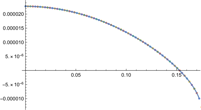
Figure 1: A plot of $\det\mathcal{M}_{v}$ with respect to the surface waves speed $v$ for a set of 100 equidistant values in the interval $[0,\widehat{v})$. It is illustrated that $\det\mathcal{M}_{v}$ is a decreasing function of the wave speed $v$.

Having the wave speed $v_{0}$, the approximation of the solution of the secular equation we find $y(0)$ as solution of the algebraic Riccati equation (7.4) in the form

$$y(0)=\left(\begin{array}[]{c}y_{1}\\ -1.263037839859903454{\rm i}\,y_{1}\\ 0.20925703711388041\,y_{1}\\ \end{array}\right),\qquad y_{1}\in\mathbb{C}.$$ (8.10)

We also have computed $\mathcal{M}_{v_{0}}$ to be

$$\mathcal{M}_{v_{0}}=\left(\begin{array}[]{ccc}0.030152425181168009480&-0.023503969977247586063{\rm i}&-0.0022270300650370918782\\ 0.023503969977247580765\,{\rm i}&0.018790427909898263031&0.0010945940135284871257\,{\rm i}\\ -0.0022270300650370918782&-0.0010945940135284891285\,{\rm i}&0.017249300922842580276\end{array}\right)$$ (8.14)

(its determinant $\det\mathcal{M}_{v_{0}}=-4.135543508749075155*10^{-13}$ is approximately zero as we expected from Theorem 7.1) and the matrix ${\mathcal{E}_{v_{0}}}={\mathcal{T}}^{-1}({\mathcal{M}_{v_{0}}}+{\rm i}\,\,{\mathcal{R}}^{T})$ is numerically approximated by

$${\mathcal{E}_{v_{0}}}=\left(\begin{array}[]{ccc}0.976843&0.238546\,{\rm i}&-0.0721487\\ 0.535545\,{\rm i}&0.228281&-1.21145\,{\rm i}\\ -2.62233&-1.28888\,{\rm i}&20.3111\\ \end{array}\right).$$ (8.18)

Having the matrix ${\mathcal{E}_{v_{0}}}$, using (7.1) we are able to find the function $y(x_{2})$. In this way, going back further with the changes of variables $y(x_{2}):=\widehat{{{\mathbbm{1}}}}^{1/2}\,z(x_{2})$ we find $z(x_{2})$ and one step back, using (6.1), we find the solution $\mathcal{U}(x_{1},x_{2},t)$, see Figure 2.

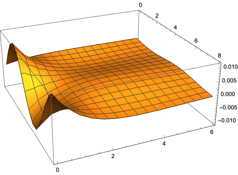
(a) Plot of the $u_{1}$-component of the displacement.

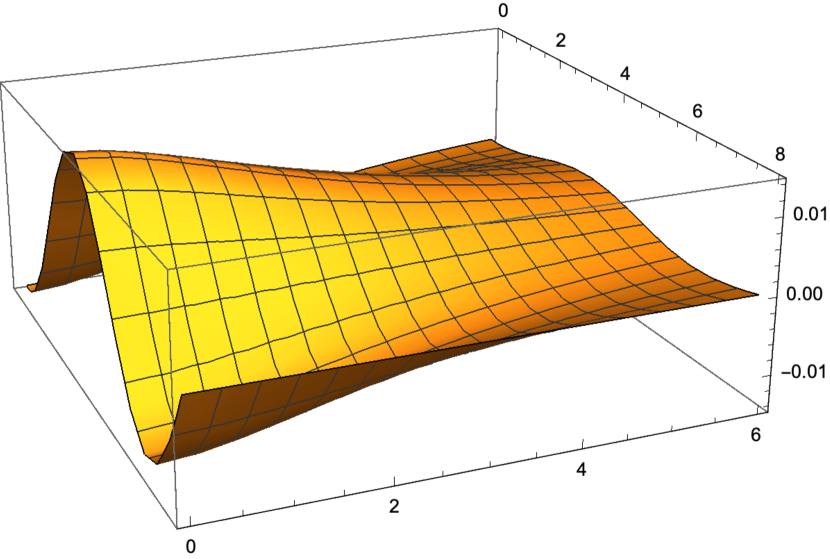
(b) Plot of the $u_{2}$-component of the displacement.

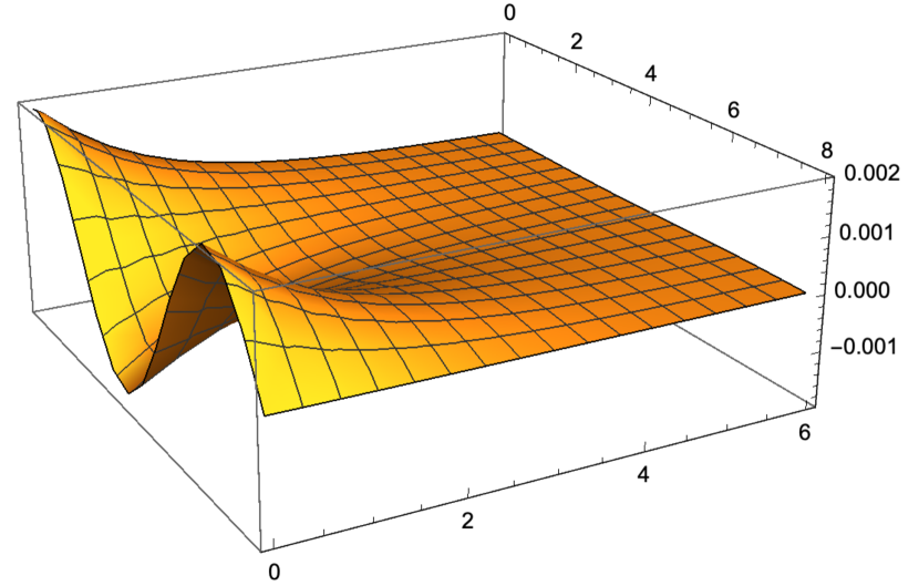
(c) Plot of the volume fraction field $\zeta$ from $P=\zeta\!\!\cdot\!\!{{\mathbbm{1}}}$.

Figure 2: The plot of the solution at time $t=1$ and for the choice $y_{1}=-{\rm i}\,$.

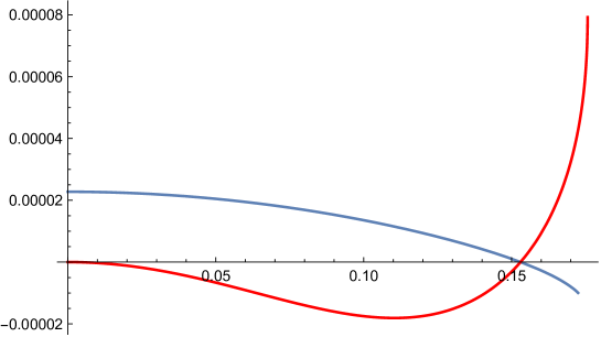
Figure 3: The plots of the approximation of $v\mapsto\det{{\mathcal{M}}}_{v}$ (blue curve) and of $v\mapsto R(v)10^{-8}$ (red curve), where $R(v)$ from (8.19) defines the secular equations from [8], with respect to the surface waves speed $v$ for the material we considered. These two different functions have the same (unique) root in the interval $[0,\widehat{v})$. We have multiplied $R(v)$ with $10^{-8}$ to have the same range plot interval of the values for both functions.

In [8] the secular equation has the form $R(c)=0$, where $c$ is the wave speed and

$$R(v)\equiv \displaystyle\left[\left(2-\frac{v^{2}}{v_{t}^{2}}\right)^{2}-4\sqrt{\left(1-\frac{v^{2}}{v_{t}^{2}}\right)\left(1-\frac{X_{1}^{2}}{k^{2}}\right)}\ \right]\sqrt{1-\frac{X_{2}^{2}}{k^{2}}}\left(-\frac{v^{2}}{v_{s}^{2}}+\frac{X_{2}^{2}}{k^{2}}\right)\vspace{1mm}$$

$$-\displaystyle\left[\left(2-\frac{v^{2}}{v_{t}^{2}}\right)^{2}-4\sqrt{\left(1-\frac{v^{2}}{v_{t}^{2}}\right)\left(1-\frac{X_{2}^{2}}{\kappa^{2}}\right)}\ \right]\sqrt{1-\frac{X_{1}^{2}}{k^{2}}}\left(-\frac{v^{2}}{v_{s}^{2}}+\frac{X_{1}^{2}}{k^{2}}\right),$$ (8.19)

where

$$X_{1,2}^{2}=X_{1,2}^{2}(\omega^{2})= \displaystyle\frac{1}{2\alpha(\lambda_{\rm e}+2\mu_{\rm e})}\Bigg{\{}{\beta}^{2}-(\xi-{\varrho_{0}}\varkappa\omega^{2})(\lambda_{\rm e}+2\mu_{\rm e})+\alpha\omega^{2}{\varrho_{0}}$$

$$\mp\sqrt{4\alpha\omega^{2}{\beta}^{2}{\varrho_{0}}+[-{\beta}^{2}+\alpha\omega^{2}{\varrho_{0}}+(\xi-{\varrho_{0}}\varkappa\omega^{2})(\lambda_{\rm e}+2\mu_{\rm e})]^{2}}\Bigg{\}}.$$ (8.20)

In [8] the uniqueness of the solution was not demonstrated and the existence of the solution of the secular equation was proven assuming the conditions (1.2). These conditions are more restrictive in comparison with the assumptions (6.29). Our analysis is valid for all materials admitting planar real wave propagation and do not enter into conflict with the necessary assumptions for classical linear elasticity. With less restrictive conditions on the constitutive parameters (connected with conditions usually imposed by the engineering community) we have proven that the solution exists and it is unique. More than that the algorithm for computing the Rayleigh wave solution presented in this paper is clear and simple without knowing in advance the analytical expressions of some eigenvalues and their associated eigenvectors (the main difficulty to obtain a complete algorithm and the proof of existence and uniqueness in the other methods).

For the coefficients considered in this paper, the conditions (1.2) from [8] are not verified (${c}_{t}^{2}\leq{c}_{s}^{2}-\displaystyle\frac{{\beta}^{2}}{{\varrho_{0}}\xi}$ is true, but  ${c}_{t}^{2}\leq\frac{\alpha}{{\varrho_{0}}\varkappa}$ is not valid). However, as one can see in Figure 3 (the red curve) the secular equation from [8] is well defined and it still has a unique solution in the interval $[0,\widehat{v})$. However, for the values of the constitutive coefficients considered, the existence and uniqueness cannot be guaranteed by the results established in [8]. From Figure 3 we can see that the same value of the propagation speed is obtained, from both forms of the secular equation (our vs. [8]). This represents another check that the algorithm proposed by us is viable and the computations are correct.

The same value $v_{0}=0.113175\,(m/s)$ is obtained as limit case in our analysis of the micro-voids model for structural steel S235 and large values of the micro-constitutive parameter $\mu_{\rm micro}$ (i.e., a large $\xi$), e.g., $\mu_{\text{micro}}=10^{7}\,\mu_{\text{macro}}=10^{7}*161.538\,\textrm{(GPa)},$ which indicates the convergence of the Rayleigh wave solution from the micro-void model to the Rayleigh wave solution from classical elasticity when $\mu_{\rm micro}\to\infty$.

References

- [1] J.D. Achenbach. Wave Propagation in Elastic Solids. North-Holland Publishing Company, Amsterdam, 1973.
- [2] S. Bauer, P. Neff, D. Pauly, and G. Starke. New Poincaré-type inequalities. Compte Rendus Acad. Sci. Paris, Ser. Math., 352(2):163–166, 2014.
- [3] S. Bauer, P. Neff, D. Pauly, and G. Starke. Dev-Div and DevSym-DevCurl inequalities for incompatible square tensor fields with mixed boundary conditions. ESAIM: Control, Optimisation and Calculus of Variations, 22(1):112–133, 2016.
- [4] Ph. Boulanger and M. Hayes. Bivectors and Waves in Mechanics and Optics, volume 4. CRC Press, 1993.
- [5] A. Bucur. Rayleigh surface waves problem in linear thermoviscoelasticity with voids. Acta Mechanica 227.4: 1199-121, 2016.
- [6] B. Brandel and R.S. Lakes. Negative Poisson’s ratio polyethylene foams. Journal of Materials Science, 36:5885–5893, 2001.
- [7] S. Burns. Negative Poisson’s ratio materials. Science, 238(4826):551–551, 1987.
- [8] S. Chiriţă and I.D. Ghiba. Inhomogeneous plane waves in elastic materials with voids. Wave Motion, 47:333–342, 2010.
- [9] S. Chiriţă and I.D. Ghiba. Strong ellipticity and progressive waves in elastic materials with voids. Proceedings of the Royal Society A: Mathematical, Physical, 466:439–458, 2010.
- [10] S. Chiriţă. Thermoelastic surface waves on an exponentially graded half-space. Mechanics Research Communications 49: 27-35, 2013.
- [11] S. Chiriţă and A. Danescu. Surface waves problem in a thermoviscoelastic porous half-space. Wave Motion, 54: 100-114, 2015.
- [12] S. Chiriţă and A. Arusoaie. Thermoelastic waves in double porosity materials. European Journal of Mechanics-A/Solids, 86: 104177, 2021.
- [13] W.D. Claus and A.C. Eringen. Three dislocation concepts and micromorphic mechanics. In Developments in Mechanics, Proceedings of the 12th Midwestern Mechanics Conference, volume 6, pages 349–358. Midwestern, 1969.
- [14] W.D. Claus and A.C. Eringen. Dislocation dispersion of elastic waves. International Journal of Engineering Science, 9:605–610, 1971.
- [15] S.C. Cowin and J.W. Nunziato. Linear elastic materials with voids. Journal of Elasticity, 13:125–147, 1983.
- [16] P.K. Currie. Rayleigh waves on elastic crystals. The Quarterly Journal of Mechanics and Applied Mathematics, 27(4):489–496, 1974.
- [17] F. Demore, G. Rizzi, M. Collet, P. Neff, and A. Madeo. Unfolding engineering metamaterials design: Relaxed micromorphic modeling of large-scale acoustic meta-structures. Journal of the Mechanics and Physics of Solids, 168:104995, 2022.
- [18] M. Destrade. The explicit secular equation for surface acoustic waves in monoclinic elastic crystals. The Journal of the Acoustical Society of America, 109(4):1398–1402, 2001.
- [19] M. Destrade. Seismic Rayleigh waves on an exponentially graded, orthotropic half-space. Proceedings of the Royal Society A: Mathematical, Physical, 463(2078):495–502, 2007.
- [20] M. Destrade, P. Martin, and T.C.T. Ting. The incompressible limit in linear anisotropic elasticity, with applications to surface waves and elastostatics. Journal of the Mechanics and Physics of Solids, 50(7):1453–1468, 2002.
- [21] A.C. Eringen. Microcontinuum Field Theories. Springer, Heidelberg, 1999.
- [22] A.C. Eringen and W.D. Claus. A micromorphic approach to dislocation theory and its relation to several existing theories. In J.A. Simmons, R. de Wit, and R. Bullough, editors, Fundamental Aspects of Dislocation Theory., volume 1 of Nat. Bur. Stand. (U.S.), Spec. Publ., pages 1023–1040. Spec. Publ., 1970.
- [23] K.E. Evans and B.D. Caddock. Microporous materials with negative Poisson’s ratios. II. Mechanisms and interpretation. Journal of Physics D: Applied Physics, 22(12):1883, 1989.
- [24] E.A. Friis, R.S. Lakes, and J.B. Park. Negative Poisson’s ratio polymeric and metallic foams. Journal of Materials Science, 23:4406–4414, 1988.
- [25] Y.B. Fu and A. Mielke. A new identity for the surface–impedance matrix and its application to the determination of surface-wave speeds. Proceedings of the Royal Society of London. Series A, Mathematical and Physical Sciences, 458 (2026):2523–2543, 2002.
- [26] Y.B. Fu and R.W. Ogden. Nonlinear Elasticity: Theory and Applications, volume 281. Cambridge University Press, 2001.
- [27] C. Galeş and S. Chiriţă. Wave propagation in materials with double porosity. Mechanics of Materials, 149: 103558, 2020.
- [28] I. D. Ghiba. On the temporal behaviour in the bending theory of porous thermoelastic plates. Zeitschrift für Angewandte Mathematik und Mechanik, 93:284–296, 2013.
- [29] I.D. Ghiba, P. Neff, A. Madeo, L. Placidi, and G. Rosi. The relaxed linear micromorphic continuum: Existence, uniqueness and continuous dependence in dynamics. Mathematics and Mechanics of Solids, 20:1171–1197, 2015.
- [30] F. Gmeineder, P. Lewintan, and P. Neff. Korn-Maxwell-Sobolev inequalities for general incompatibilities. arXiv preprint arXiv:2212.13227, 2022.
- [31] F. Gmeineder, P. Lewintan, and P. Neff. Optimal incompatible Korn–Maxwell–Sobolev inequalities in all dimensions. Calculus of Variations and Partial Differential Equations, 62(6):1–33, 2023.
- [32] M.A. Goodman and S.C. Cowin. A continuum theory for granular materials. Archive for Rational Mechanics and Analysis, 44(4):249–266, 1972.
- [33] J.N. Grima, R. Gatt, N. Ravirala, A. Alderson, and K.E. Evans. Negative Poisson’s ratios in cellular foam materials. Materials Science and Engineering: A, 423(1-2):214–218, 2006.
- [34] H. Hayes and R. Rivlin. A note on the secular equation for Rayleigh waves. Zeitschrift für angewandte Mathematik und Physik, 13:80–83, 1962.
- [35] M. Hayes. Inhomogeneous plane waves. In The Breadth and Depth of Continuum Mechanics, pages 247–285. Springer, 1986.
- [36] M. Hayes and R.S. Rivlin. A note on the secular equation for Rayleigh waves. Zeitschrift für angewandte Mathematik und Physik, 13(1):80–83, 1962.
- [37] D. Ieşan. A theory of thermoelastic materials with voids. Acta Mechanica, 60:67–89, 1986.
- [38] D. Ieşan and M. Ciarletta. Non-Classical Elastic Solids. Longman Scientific and Technical, Harlow, Essex, UK, Inc., New York, 1993.
- [39] J.W. Jiang and H.S. Park. Negative Poisson’ ratio in single-layer black phosphorus. Nature Communications, 5(1):4727, 2014.
- [40] H. Khan, I.D. Ghiba, A. Madeo, and P. Neff. Existence and uniqueness of Rayleigh waves in isotropic elastic Cosserat materials and algorithmic aspects. Wave Motion, 110:102898, 2022.
- [41] H.W. Knobloch, A. Isidori, and D. Flockerzi. Topics in Control Theory, volume 22. Birkhäuser, 2012.
- [42] R.S. Lakes. Foam structures with a negative Poisson’s ratio. Science, 235(4792):1038–1040, 1987.
- [43] R.S. Lakes. Advances in negative Poisson’s ratio materials. Advanced Materials, 5(4):293–296, 1993.
- [44] R.S. Lakes, T. Lee, A. Bersie, and Y.C. Wang. Extreme damping in composite materials with negative-stiffness inclusions. Nature, 410(6828):565–567, 2001.
- [45] J. Lankeit, P. Neff, and D. Pauly. and applications to elasticity. Zeitschrift für Angewandte Mathematik und Physik, 64:1679–1688, 2013.
- [46] M. Lazar and H. Kirchner. Cosserat (micropolar) elasticity in Stroh form. International Journal of Solids and Structures, 42(20):5377–5398, 2005.
- [47] P. Lewintan, S. Müller, and P. Neff. Korn inequalities for incompatible tensor fields in three space dimensions with conformally invariant dislocation energy. Calculus of Variations and Partial Differential Equations, 60:1–46, 2021.
- [48] P. Lewintan and P. Neff. Nečas–Lions lemma revisited: An -version of the generalized Korn inequality for incompatible tensor fields. Mathematical Methods in the Applied Sciences, 44(14):11392–11403, 2021.
- [49] X.-F. Li. On approximate analytic expressions for the velocity of Rayleigh waves. Wave Motion, 44:120–127, 2006.
- [50] A. Madeo, P. Neff, I. D. Ghiba, L. Placidi, and G. Rosi. Band gaps in the relaxed linear micromorphic continuum. Zeitschrift für Angewandte Mathematik und Mechanik, 95(9):880–887, 2015.
- [51] A. Madeo, P. Neff, I. D. Ghiba, L. Placidi, and G. Rosi. Wave propagation in relaxed linear micromorphic continua: modelling metamaterials with frequency band-gaps. Continuum Mechanics and Thermodynamics, 27:551–570, 2015.
- [52] A. Madeo, P. Neff, I.D. Ghiba, and G. Rosi. Reflection and transmission of elastic waves in non-local band-gap metamaterials: a comprehensive study via the relaxed micromorphic model. Journal of the Mechanics and Physics of Solids, 95:441–479, 2016.
- [53] P.G. Malischewsky. Comment to “A new formula for velocity of Rayleigh waves” by D. Nkemzi [Wave Motion 26 (1997) 199-205]. Wave Motion, 31:93–96, 2000.
- [54] A. Mielke and Y.B. Fu. Uniqueness of the surface-wave speed: a proof that is independent of the Stroh formalism. Mathematics and Mechanics of Solids, 9(1):5–15, 2004.
- [55] A. Mielke and P. Sprenger. Quasiconvexity at the boundary and a simple variational formulation of Agmon’s condition. Journal of Elasticity, 51(1):23–41, 1998.
- [56] R.D. Mindlin. Micro-structure in linear elasticity. Archive for Rational Mechanics and Analysis, 16:51–77, 1964.
- [57] V.G. Mozhaev. Some new ideas in the theory of surface acoustic waves in anisotropic media. In IUTAM Symposium on Anisotropy, Inhomogeneity and Nonlinearity in Solid Mechanics, pages 455–462, 1995.
- [58] P. Neff, A. Madeo, G. Barbagallo, M.V. d’Agostino, R. Abreu, and I.D. Ghiba. Real wave propagation in the isotropic-relaxed micromorphic model. Proceedings of the Royal Society A: Mathematical, Physical and Engineering Sciences, 473(2197):20160790, 2017.
- [59] P. Neff, I. D. Ghiba, M. Lazar, and A. Madeo. The relaxed linear micromorphic continuum: well-posedness of the static problem and relations to the gauge theory of dislocations. The Quarterly Journal of Mechanics and Applied Mathematics, 68:53–84, 2015.
- [60] P. Neff, I. D. Ghiba, A. Madeo, L. Placidi, and G. Rosi. A unifying perspective: the relaxed linear micromorphic continuum. Continuum Mechanics and Thermodynamics, 26:639–681, 2014.
- [61] P. Neff, D. Pauly, and K.J. Witsch. A canonical extension of Korn’s first inequality to motivated by gradient plasticity with plastic spin. Compte Rendus Acad. Sci. Paris, Ser. Math., 349:1251–1254, 2011.
- [62] P. Neff, D. Pauly, and K.J. Witsch. Maxwell meets Korn: a new coercive inequality for tensor fields in with square-integrable exterior derivative. Mathematical Methods in the Applied Sciences, 35:65–71, 2012.
- [63] P. Neff, D. Pauly, and K.J. Witsch. Poincaré meets Korn via Maxwell: Extending Korn’s first inequality to incompatible tensor fields. Journal of Differential Equations, 258:1267–1302, 2015.
- [64] D. Nkemzi. A new formula for the velocity of Rayleigh waves. Wave Motion, 26:199–205, 1997.
- [65] D. Nkemzi. A simple and explicit algebraic expression for the Rayleigh wave velocity. Mechanics Research Communications, 35:201–205, 2008.
- [66] J.W. Nunziato and S.C. Cowin. A nonlinear theory of elastic materials with voids. Archive for Rational Mechanics and Analysis, 72:175–201, 1979.
- [67] P. Puri and S.C. Cowin. Plane waves in linear elastic materials with voids. Journal of Elasticity, 15(2):167–183, 1985.
- [68] M. Rahman and J.R. Barber. Exact expression for the roots of the secular equation for Rayleigh waves. ASME Journal of Applied Mechanics, 62:250–252, 1995.
- [69] Lord Rayleigh. On waves propagated along the plane surface of an elastic solid. Proceedings of the London Mathematical Society, 17:4–11, 1885.
- [70] G. Rizzi, M.V. d’Agostino, P. Neff, and A. Madeo. Boundary and interface conditions in the relaxed micromorphic model: Exploring finite-size metastructures for elastic wave control. Mathematics and Mechanics of Solids, 27(6):1053–1068, 2022.
- [71] G. Rizzi, P. Neff, and A. Madeo. Metamaterial shields for inner protection and outer tuning through a relaxed micromorphic approach. Philosophical Transactions of the Royal Society A, 380(2231):20210400, 2022.
- [72] G. Rizzi, D. Tallarico, P. Neff, and A. Madeo. Towards the conception of complex engineering meta-structures: Relaxed-micromorphic modelling of low-frequency mechanical diodes/high-frequency screens. Wave Motion, 113:102920, 2022.
- [73] G. Rizzi, J. Voss, P. Neff, and A. Madeo. Modeling a labyrinthine acoustic metamaterial through an inertia-augmented relaxed micromorphic approach. Mathematics and Mechanics of Solids, 28 (10):2177-2201, 2023.
- [74] G. Rizzi, L.A. Perez Ramirez and A. Madeo. Multi-element metamaterials design through the relaxed micromorphic model. In Sixty Shades of Generalized Continua: Dedicated to the 60th Birthday of Prof. Victor A. Eremeyev, pages 579–600. Springer, 2023.
- [75] L. Rothenburg, A.I. Berlin, and R.J. Bathurst. Microstructure of isotropic materials with negative Poisson’s ratio. Nature, 354(6353):470–472, 1991.
- [76] A.N. Stroh. Dislocations and cracks in anisotropic elasticity. Philosophical Magazine, 3(30):625–646, 1958.
- [77] A.N. Stroh. Steady state problems in anisotropic elasticity. Journal of Mathematical Physics, 41(1-4):77–103, 1962.
- [78] J.L. Synge. Elastic waves in anisotropic media. Journal of Mathematical Physics, 35(1-4):323–334, 1956.
- [79] R.M. Taziev. Dispersion relation for acoustic waves in an anisotropic elastic half-space. Akustičeskij Žurnal, 35(5):922–928, 1989.
- [80] T.C.T. Ting. An explicit secular equation for surface waves in an elastic material of general anisotropy. The Quarterly Journal of Mechanics and Applied Mathematics, 55(2):297–311, 2002.
- [81] T.C.T. Ting. Secular equations for Rayleigh and Stoneley waves in exponentially graded elastic materials of general anisotropy under the influence of gravity. Journal of Elasticity, 105:331–347, 2011.
- [82] T.C.T. Ting. Surface waves in an exponentially graded, general anisotropic elastic material under the influence of gravity. Wave Motion, 48:335–344, 2011.
- [83] P.C. Vinh and P.G. Malischewsky. An approach for obtaining approximate formulas for the Rayleigh wave velocity. Wave Motion, 44:549–562, 2007.
- [84] P.C. Vinh and P.G. Malischewsky. Improved approximations of the Rayleigh wave velocity. Journal of Thermoplastic Composite Materials, 21:337–352, 2008.
- [85] P.C. Vinh and R.W. Ogden. On formulas for the Rayleigh wave speed. Wave Motion, 39:191–197, 2004.
- [86] Y. Yang, D. Cormier, H. West, O. Harrysson, and K. Knowlson. Non-stochastic ti–6al–4v foam structures with negative Poisson’s ratio. Materials Science and Engineering: A, 558:579–585, 2012.