T-COL: Generating Counterfactual Explanations for General User Preferences on Variable Machine Learning Systems

Abstract

Machine learning (ML) based systems have been suffering a lack of interpretability. To address this problem, counterfactual explanations (CEs) have been proposed. CEs are unique as they provide workable suggestions to users, in addition to explaining why a certain outcome was predicted. However, the application of CEs has been hindered by two main challenges, namely general user preferences and variable ML systems. User preferences, in particular, tend to be general rather than specific feature values. Additionally, CEs need to be customized to suit the variability of ML models, while also maintaining robustness even when these validation models change. To overcome these challenges, we propose several possible general user preferences that have been validated by user research and map them to the properties of CEs. We also introduce a new method called Tree-based Conditions Optional Links (T-COL), which has two optional structures and several groups of conditions for generating CEs that can be adapted to general user preferences. Meanwhile, a group of conditions lead T-COL to generate more robust CEs that have higher validity when the ML model is replaced. We compared the properties of CEs generated by T-COL experimentally under different user preferences and demonstrated that T-COL is better suited for accommodating user preferences and variable ML systems compared to baseline methods including Large Language Models.

Keywords Interpretability  $\cdot$ Machine learning (ML)  $\cdot$ Explainable artificial intelligence (XAI)  $\cdot$ User preferences  $\cdot$ Variable machine learning systems  $\cdot$ Counterfactual explanations

1 Introduction

Counterfactual explanations (CEs) offer a special answer to the lack of interpretability in widely used and well-performing machine learning (ML) systems, with important implications for ML interpretability [1, 2, 3, 4] and AI security [5, 6, 7]. As first proposed by [8], CEs entail as few as possible changing the original data points (named query sample) to reach the desired class, answering the question “How to change $x$ to $\tilde{x}$ would cause the classifier to classify $y$ to $\tilde{y}$?”. For example, a loan decision ML system might reject a loan request from a user with a profile such as {age: 24, education: bachelor, job: service, institution: private}. Conventional methods might state that “your job type is service-oriented, which led to the rejection of your loan request”, whereas a CE would state that “working in a professional job will result in your application being approved”. This example illustrates that CEs reveal what differences in an instance can lead to a desired outcome. The complete examples of CE can be seen in Table 1, showing the two ways in which a loan can be successfully approved (loan is “True”) for a query sample where the loan request is not approved (loan is “False”). Due to the importance of interpretability and the uniqueness of CE, many researchers have worked on the generation of CEs[9, 10, 11, 5, 12]. CEs are also used in various ML-based systems [13, 14, 15, 16, 17, 18, 19] and has garnered considerable attention within various ML communities[20, 10, 21, 22, 23, 24, 25, 26]. However, the further application of CE still faces many challenges. The possibility of CEs is perceived as manipulative from a security point of view, as discussed in [27]. The robustness of the CEs is analyzed in [28] and [29].

Table 1: Explambles of counterfactual explanations

	age	job	education	institution	sex	work_hours	income	loan
query sample	24	Service	Bachelor	Private	Male	40	15,000	False
CE_1	27	Professional	Master	Private	Male	40	35,000	True
CE_2	30	Manage	Bachelor	Private	Male	75	50,000	True

Twelve key challenges have been listed in [30] for CEs in practical applications and industrial deployments. Our work specifically addresses Challenges 3 and 7 of these. On the one hand, challenge 3 (ML models are not static) states that the validation model in CE generation is not fixed. Most research on CEs assumes that the validation models for sample classification are fixed and do not change over time while ML systems are frequently upgraded and changed in practice. Currently, only a few works have investigated the robustness of CEs from a sample perspective, but no work has focused on the robustness of CEs on variable ML systems. On the other hand, challenge 7 (Capturing personal preferences) requires that the generation methods for CEs should have the ability to capture user preferences. Some researchers [31] have attempted to incorporate user preferences into CEs by adding constraints on feature values. Another method [32] built an interactive interface that allows users to select and set the range of feature values or tendencies for the features. Nevertheless, there is still much work to be done in developing CEs that can adapt to immutable features and variable but infeasible features. Furthermore, such superficial user preferences for feature values can only capture the user’s tendency for a single task and are difficult to adapt to complex tasks in real applications.

In this paper, we presuppose possible general user preferences that do not usually change with specific tasks. To demonstrate the validity of these general user preferences and the proportion of these preferences covered, we designed questionnaires and invited students from different majors and different grades to answer them. Then we set up optional structures to accommodate these general user preferences. In addition, we used these two optional structures to set up a group of conditions to generate CEs that are more robust on variable ML systems.

To address the current limitations of generating CEs in ML, we propose Tree-based Conditions Optional Links (T-COL) to generate CEs capturing general user preferences. First, a feature-based approach generates CEs by selecting combinations of feature values from prototype cases with the target category and the query sample. Moreover, to improve the adaptability of CEs to variable ML systems and better capture user preferences, we offer two optional structures for user preferences. We have predefined several general user preferences, linked them to the properties of CEs, and mapped the relevant properties to the optional structure of T-COL. To assess the adaptability of CEs to general user preferences, we compared the properties of CEs related to user preferences and proposed centrality to evaluate the proximity of CEs to the cluster of the desired category samples. In the two optional structures of T-COL, we construct a group of conditions considering the variable ML systems. These conditions lead to generating CEs with higher robustness and truthfulness that can better cope with variable ML systems. Furthermore, we propose data fidelity to evaluate the adaptability of CEs to variable ML systems using the classification results of different models for the generated CEs.

Our work has the following primary contributions:

• We link predefined general user preferences to the properties of CEs and propose a feature-based approach T-COL with optional structures to capture these preferences. Furthermore, we define centrality as a complement to existing properties to evaluate the ability of CEs to accommodate general user preferences.

• We propose feature selection conditions that motivate the generation of more effective and robust CEs and data fidelity to measure the adaptability of CEs to variable ML systems.

• Extensive experiments have shown that the CEs generated by our proposed T-COL method are better adapted to variable ML models and general user preferences.

The remaining parts of this paper are arranged as follows. Section 2 surveys related works in terms of both generation methods and the properties of CE. Section 3 defines general user preferences, describes the definition of the CE generation problem, and provides a theoretical analysis of how T-COL secures the properties of CEs. Section 4 expounds on how T-COL generates CEs and the general user preferences’ connection to the properties of CEs are presented. Section 5 presents experimental results under different user preferences and comparisons with other popular methods and Spark as a representative of LLMs. At last, we draw some conclusions in Section 6.

2 Releated Work

2.1 Counterfactual Explanation Generation Approaches

The two main categories of CE generation approaches can be divided into optimization-based and feature-based methods, depending on the generation methodology.

Optimization-based approaches generate CEs by perturbing the original data points so that they cross the decision boundary and are classified as the desired class. This intuitive idea has been used by many researchers to model different properties as optimization problems and design different optimization methods. For example, [8] introduced the concept of CE and constructed an optimization objective based on the distance between the counterfactual sample and the query sample and the prediction of the counterfactual sample made by the decision model, which was optimized by adam[33]. There are also researchers who have formalized most of the properties introduced in previous work on CE as different constraints on the optimization objective and solved for the CE using constrained optimization learning [34]. Optimization objectives can be solved using methods such as integer coding [35] and gradient descent [36]. Another optimization-based method involves solving for perturbations about query samples in the data space, where perturbations can be learned in the discrete data space by calculating diversity-enforcing losses[37] or finding the sample points most relevant to the target CE from the data space to construct counterfactual pairs, each counterfactual pair consists of a query sample and a selected target sample, and deriving the set of CEs from the counterfactual pairs by an iterative approach[38]. In addition, the solution of the CE problem has been formalized as an optimization problem for a non-monotonic submodular function in [39] which can be solved by randomization methods.

The methods used to solve optimization problems often operate on continuous values, leading to CEs that include unfeasible or understandable but not generally perceived features, such as half a master’s degree getting a loan application or a person being 35.8 years old having a higher income. As a consequence, feature-based methods have been developed to generate CEs based on features selected from the sample set or the full data space. For example, [40] constructed counterfactual pairs using good cases in the target category and used the different feature values in the counterfactual pairs as the corresponding feature values to compose CEs. Another method is diverse CEs by reusing the $k$-nearest neighbor case pairs[41]. And [42] generated CEs of the bird figures by replacing features in the query samples at the corresponding location with features in the target category samples. In an extension of the case-based approach, continuous features are transformed into categorical alternatives in [25] to generate more effective CEs from the psychological perspective.

Based on the characteristics of these two types of approaches, we adopt the feature-based idea to design the CE generation method. Compared to the optimization-based approach, it can better ensure the feasibility of CEs.

2.2 Attributes and Evaluation Metrics

How to evaluate the quality or explanatory effect of CEs has also received a great deal of attention from researchers. The properties and evaluation metrics regarding CE, and even regarding the properties of the interpreter, have been proposed.

[11] formally and systematically presented the properties of CEs, containing metrics such as validity, actionability, and sparsity, providing metrics for research in related fields and standards for the application of CEs. Several properties on CE are expressed formally in [34] and defined in the form of formulas as constraints in the process of generating CEs. [10] provided a very comprehensive summary of properties, presenting the properties associated with CE in terms of both CE and interpreters, respectively.

In addition, some researchers have also assessed CEs and interpreters from perspectives other than their properties. In order to improve the fairness of CEs, it is proposed in [43] that the robustness of CEs must first be improved, and plausible CEs are defined to achieve this. [44] also discusses the research work on CE from a robustness perspective. [45] presented an analysis from a psychological and computational perspective, proposing requirements for distributionally faithful and instance-guided CEs.

Building on these studies on properties and evaluation metrics, [30] presents 12 challenges for CE of future developments. However, there is currently little research on Challenge 3 and Challenge 7. Therefore, this paper proposes to generate CEs under the conditions of general user preferences variable ML models, and corresponding metrics to evaluate them.

3 The User Preferences and problem definition

3.1 Pre-defined General User Preferences

In previous work, only the user’s requirements for a particular writing feature were considered, without a general consideration of the user’s individual personality and preferences. However, in practical applications and deployments, users may not be able to express their requirements for specific features with certainty but rather express their preference for a certain practice or a certain type of CEs. For example, users may be more likely to say “I want an easy way to get approved for a loan” rather than “I want the type of work to be professional or managerial”. It is therefore important to dig more generally into the links between user preferences and the properties of CEs. However, these general user preferences are different from the simple requirements for feature values, which cannot be added directly to optimization methods or feature selection methods that solve CEs of constraints. Therefore, we predefine several possible general user preferences and mine them for connections to the properties of CEs.

Our predefined general user preferences are as follows.

• I prefer to focus on a few things.

• I wish it is easier to do.

• I think the safer option is better.

• I hope there are similar success stories.

• The majority of people are in the situation I would like to take.

The user preferences listed above are more general and have greater research value and significance than simple constraints on certain feature values. However, such general user preferences cannot simply be represented on feature values and need to be linked to the properties of the CEs so that they can be captured in the generation of CEs.

In order to verify the reasonableness and completeness of the general user preferences defined in this paper and the tendency of users to have different preferences in the application scenarios, we designed a questionnaire to simulate the process of selecting user preferences in the process of generating CEs and invited students from different majors and grades to answer the questionnaire. The results of the research on user preferences are shown in Fig. 1.

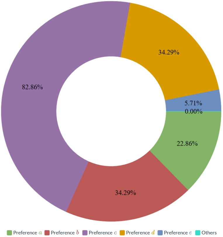
Figure 1: Percentage of general user preferences selected. We set up a scenario with a magic machine in the questionnaire, where the magic machine is able to provide options to help a person achieve a goal, which is consistent with the idea of CE. In addition to the five user preferences we defined, we allowed user-defined preferences to be supplemented. Each respondent is asked to select or supplement a minimum of one preference and a maximum of two preferences. Different colors in the figure represent the proportion of different user preferences selected by respondents.

As shown in Fig. 1, no respondents supplemented other user preferences on their own, and it can be assumed that our predefined general user preferences can satisfy the requirements of most users without considering the difficulty difference between the two operations of supplementing and selecting. It is also important to note that 82.86% of the respondents believe that user preference $c$, a more reliable solution, is very important. Therefore, we provide further analysis of the performance of CEs on preference $c$. In addition, the results of the user research proved the value of the two main problems we presented.

3.2 Definition of The Generation Problem of Counterfactual Explanations

In order to generate CEs with a higher degree of feasibility, we use the feature-based idea to design the CE generation method. The feature-based CE generation method essentially initializes the CEs as blank samples, i.e. the features are consistent with the rest of the sample but all feature values are empty, and then selects feature values from the local or global feature space to populate the CEs with the corresponding features. Let $x$ denote a query sample and $\hat{x}$ denote an arbitrary combination of features, then the combination of features in CEs denoted as $\tilde{x}$ is the solution to (1).

$$\tilde{x}=\arg\min_{\hat{x}}(|\operatorname{\textbf{M}}(\hat{x})-\tilde{y}|+\operatorname{\textbf{d}}(\hat{x},x))$$ (1)

where $\tilde{y}$ is the target class, $\operatorname{\textbf{M}}$ denotes the ML model and $\operatorname{\textbf{M}}(\cdot)$ denotes the classification result of the model on the sample. In addition, $\operatorname{\textbf{d}}$ denotes the distance between the counterfactual sample and the query sample, which can be calculated using any distance calculation function, such as Euclidean distance, Manhattan distance, etc. The first component represents the absolute value of the error between the classification result of the ML model $\operatorname{\textbf{M}}$ for the current combination of features and the desired category. Reducing this value forces the solved CEs to reach the target category. The second part represents the distance between the current feature combination and the query sample, motivating the CEs generated to be closer to the query sample. The two properties in (1) accompany the birth of CE and are the most essential ones, to which more or more external constraints can be added depending on the different requirements for the CEs.

The main part of feature-based CE generation is the process of feature value selection. The selection of feature values from different cases which are selected samples in the target category provides better assurance and control over the properties of the CEs and has therefore received more attention than the selection of feature values from the full feature space. To better capture general user preferences and construct links to the properties of CEs, we utilise the case-based ideology to design CE generation methods. In addition to the selection of feature values, the case-based approach requires the selection of good cases in the target category to provide a range of optional eigenvalues.

Based on this, our CE generation method has the following main components:

• Case selection: Select good samples from all samples in the target category based on the requirements for CEs as prototype cases, providing a range of feature values to choose from when generating CEs.

• Feature values selection: Select a set or combination of sets of feature values from a sample of cases and the query sample.

• Feature values filling: The selected feature values are filled into the blank CEs while ensuring feature consistency, and the complete CEs are obtained after validation.

Of the three processes listed above, the feature values filling process is fixed, where case selection and feature values selection have high correlations with the properties of CEs, which can be linked to general user preferences.

3.3 How to Ensure The Properties of Counterfactual Explanations

Having identified the idea of generating CEs, we further analyzed how the various properties of CEs can be ensured when designing a CE generation method.

• Validity: This property requires CEs to be classified as the target category by the decision system, i.e. the validation model. To ensure validity, we bootstrap the generation of CEs by selecting good cases in the target category and validating them with the model to filter out invalid combinations of feature values after they have been generated.

• Actionability: Also known as feasibility, actionability requires that impractical feature values do not occur and that immutable and variable infeasible features do not change. In the process of generating CEs, the feature-based approach selects feature values from existing feature values and does not produce impractical feature values. We avoid generating infeasible CEs by fixing the feature values that should not change to those of the query samples.

• Sparsity: Researchers have concluded that the number of different feature values between CEs and the query sample should be as small as possible. We guide the generation of CEs by selecting samples of the target category that have less different feature values from the query samples as prototype cases to improve the sparsity of the CEs generated.

• Data Manifold closeness: The generated CEs should be located in the feature space of the whole data to ensure they are more realistic. The CEs generated by the case-based approach lie between the prototype cases and the query sample, so they must lie in the complete feature space which is a convex polyhedron.

• Efficient: Generating CEs requires expensive computational resources for extensive post-hoc computations, which need to be reduced to improve the efficiency of CE generation in order to better application.

• Proximity: CEs that are closer to the query sample are usually considered easier to implement, a property that has been important since CE was proposed. We improve the proximity of the CEs by selecting samples of the target category that are closer to the query sample as prototype cases.

• Coherence: After encoding the classification features and performing the relevant calculations to generate the CEs, the original feature values need to be mapped back to obtain consistent CEs. We record the origin of the selected feature values by a sequence of markers and finally extract the feature values from the corresponding samples based on the sequence of markers to ensure consistency.

• Diversity: Generating diverse CEs can provide users with a variety of options, which is a property of interest to many researchers. We generate multiple CEs of the query sample by selecting multiple good cases separately.

The above analyses how to secure the existing properties of CEs that have received widespread attention. The feasibility of our idea is analyzed from a theoretical point of view. In the next section, we will specifically describe the proposed T-COL and analyze how it solves the two problems.

To better measure the adaptability of CEs to variable ML systems, we also propose a new property in addition to the above, called data fidelity. It is defined as shown in (2).

$$data\ fidelity=\frac{\displaystyle\sum^{m}_{i=1}(w_{i}\times p_{i})}{\displaystyle\sum^{m}_{i=1}w_{i}}$$ (2)

The aim of the proposed data fidelity is to evaluate the validity of CEs when ML systems are changed, i.e. the ability of CEs to remain classified as the target class when the ML models change. Therefore, we used the classification results of CEs by third-party models (Arbitrary ML classification models) to assess the data fidelity of CEs. In (2), $m$ donates the number of third-party models and $w_{i}$ denotes the weight of the third-party models. The more discriminative it is of the original data, i.e. its classification accuracy as evaluated by the $F1-score$, the greater its corresponding weight. Meanwhile, $p_{i}$ denotes the classification accuracy of the third-party models for CEs expressed as $F1-score$. The $F1-score$ is calculated as shown in (3),

$$F1-score=\frac{2\times P\times R}{P+R}\times 100$$ (3)

where $P$ and $R$ denote the accuracy and recall of the ML models. The $F1-score$ is commonly used to assess the performance of a classifier, which we use to indicate the degree of endorsement of whether CEs belong to the target class. Data fidelity helps to analyze the effectiveness and stability of CEs in the face of variable ML systems and provides a new metric for the study of CE that facilitates their application and deployment. We show the data fidelity of CEs generated by different methods in Section 5.

In addition, to assess general user preferences $d$ and $e$, we propose the evaluation metric centrality, expressed as the distance between the CE and the cluster centroid of the target category samples, in the form of (4),

$$centrality=\frac{1}{n}\times\displaystyle\sum^{n}_{i=1}\frac{\operatorname{d}(\dot{x}_{i},\check{x})}{\operatorname{d}(\dot{x}_{i},\tilde{x})}$$ (4)

where $\check{x}$ is the cluster centroid, $\dot{x}$ denotes the $n$ sample points in the immediate vicinity of the cluster centroid, and $\tilde{x}$ denotes the CE. A higher centrality of the CE indicates that the more similar it is to the majority of the target class samples, the better it matches the general user preferences.

4 Proposed T-COL

In this section, we analyze the relationship between general user preferences and the properties of CEs and map the relationship to the CE generation process of T-COL. T-COL captures general user preferences by selecting suitable conditions and generates CEs that match user preferences using processes such as feature segmentation, feature value selection, and feature value padding. T-COL first constructs local greedy trees using subsets of the divided local feature values to represent arbitrary local combinations of feature values. In addition, locally optimal combinations of feature values are selected on the local greedy tree according to predefined rules. Afterward, T-COL joins several local greedy trees in feature order, and the linking tree stitches the feature value selection paths obtained from the local greedy trees into a complete feature value selection path for selecting the feature values to be populated into the CE.

4.1 General User Preference Analysis

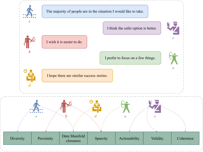
Figure 2: The relationship between general user preferences and the properties of CEs. The different colored people indicate users with different personalities and who have different general user preferences. The green rectangle indicates the properties of CEs and the different colored dashed arrows indicate the links between the general user preferences and the properties of CEs. The figure shows the properties of CEs that are primarily associated with these general user preferences. For example, The lumberjack wants CEs to be easier to do, requiring that the generated CEs be closer to the query sample and that the number of different feature values should be as small as possible, i.e. with higher sparsity.

General user preferences are more like the personalities of the users rather than just requirements for a particular feature in a task. However, general user preferences can not be achieved directly by imposing constraints on the generation of CEs. Therefore, we first analyze the connection between general user preferences and the properties of CEs, as shown in Fig. 2.

User preference $a$ requires as few different features as possible between CEs and the query sample so that the user can focus on changing a small number of feature values, requiring a higher degree of sparsity in the generated CEs. User preference $b$ requires CEs to be easier to achieve, which intuitively means that the distance between CEs and the query sample should be as close as possible, placing a higher demand on the proximity of CEs. User preference $c$ indicates that the user wants to choose CEs that provide more secure solutions to achieve their needs, which requires a higher level of validity and data fidelity of CEs. It is also necessary to ensure that the CEs have a higher degree of feasibility, validity, and consistency. The user preference $d$ indicates that the user wants similar success cases, which require CEs to be located in a convex hull feature space made up of existing data. User preference $e$ indicates that the user wishes to take the option chosen by the majority, i.e. CEs need to be representative and located in the feature space where the sample points are concentrated.

Based on the design ideas of the CE generation method presented earlier, the prototype case selection and feature value selection processes can be set up with different rules to suit general user preferences. On the basis of this, we further specify the concrete implementation of the two optional structures corresponding to general user preferences for T-COL.

We present the implementation of each predefined general user preference in two optional structures separately.

• For general user preference $a$, CEs with a smaller number of distinct feature values need to be generated. Therefore, when selecting the prototype cases we chose samples of the target category with fewer different feature values from the query sample as the prototype cases. In addition, we define the feature value selection rule “few-counterfactual score (fcs)” as shown in (5).

  $$fcs=\operatorname{sigmod}(\cos({\hat{x},\ddot{x}}))\times\displaystyle\sum^{n}_{i=1}\operatorname{equ}(|\hat{x}_{i}-x_{i}|)$$ (5)

  $$\operatorname{equ}(x)=\begin{cases}0,&x=0\\ 1,&x\neq 0\end{cases}$$ (6)

  where $n$ denotes the number of features in each sample, $\ddot{x}$ denotes a prototype case, and (6) maps the difference in feature values to the difference in the number of feature values. The first component in (5) indicates the degree of resemblance between the current combination of feature values and the prototype case which means the probability that the current combination of feature values will be classified as the target class by the ML model, and the second part indicates the number of feature values that differ between the current combination of feature values and the query sample. fcs combinations with the maximum or greater than a given threshold can be interpreted as alternate counterfactuals.

• For general user preference $b$, we choose the nearest target category sample to the query sample as the prototype case. And “near-counterfactual score (ncs)” is designed as the feature values selection rule, which is calculated as (7).

  $$ncs=\frac{\operatorname{sigmoid}(\cos(\hat{x},\ddot{x}))}{\exp(\operatorname{d}(\hat{x},x))}$$ (7)

  The above equation consists of two parts, the upper part represents the degree of similarity between the current combination of feature values and the prototype sample, and the lower part represents the distance between the current combination of feature values and the query sample. In addition, depending on the user’s preference for CEs, we scale values using the exponential and sigmoid functions respectively.

• To accommodate user preference $c$, the sample with the highest probability of being classified into the target category by the given ML model was chosen as the prototype case. In addition, we also follow the previous approach and give evaluation metrics for the combination of feature values in (8).

  $$rss=\frac{\exp(\cos(\hat{x},\ddot{x}))}{\operatorname{sigmoid}(\operatorname{d}(\hat{x},x))}$$ (8)

  To allow the generated CEs to be more securely classified as target categories, “relative similarity score (rss)” amplified the importance of the similarity between the combination of feature values and the prototype case in (8).

• In order to match the requirements of user preference $d$, the target category sample with the highest similarity to the query sample was selected as the prototype case, and rss was used as the metric to evaluate the combination of feature values.

• The largest number of samples can be found at the cluster centroid, so the sample near the cluster centroid is the optimal solution with respect to user preference $e$. Furthermore, rss is equally applicable to the evaluation of the combination of eigenvalues under such conditions.

4.2 Overall Design of T-COL

According to the previous analysis, the process of generating CEs is divided into two main parts: case selection and feature values selection, and T-COL is designed based on this ideology. In order to improve the efficiency of the generation of CEs, we use a partitioning strategy that divides the generation process of CEs into a selection process of several combinations of local feature values. We first construct local greedy trees (see 4.3) representing the local combination of feature values and filter the locally optimal paths for the combination of feature values based on the given metrics. Finally, all the paths filtered by the local greedy tree are linked, and the feature space of the CE is populated by selecting features from the prototype case and the query sample respectively according to the complete feature value selection path (see 4.4 and 4.5). The overall structure is shown in Fig. 5.

4.3 Local Greedy Tree

A local greedy tree (LGT) is a tree structure used to represent the combination of local feature values of the prototype case $P$ and the query sample $S$. The nodes of the tree consist of the feature values of the prototype and query samples.

For example, when the encoded feature vectors of the first three features of the two samples are $\ddot{x}_{l}=[0.6,0.89,0.49]$ and $x_{l}=[0.8,0.45,0.87]$ respectively, a local greedy tree can be constructed as shown in Fig. 3. The orange nodes indicate the eigenvalue encoding of the prototype case $P$ and the green nodes indicate the eigenvalue encoding of the query sample $S$. The yellow paths indicate the prototype case’s local feature subsets, and the blue paths indicate the local feature subsets of the query sample, while black paths only connect any combination of feature values.

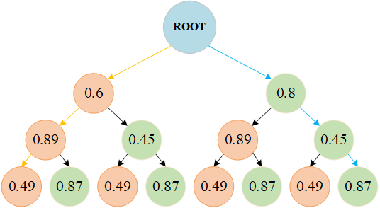
Figure 3: An example of a local greedy tree. The depth of the tree is equal to the number of elements in the local feature subset, and the nodes at each level store the feature values of the query sample and the prototype case, respectively. By traversing each path of the local greedy tree, several sets of local feature combinations can be obtained, and the optimal local feature combination can be selected according to the preset rules.

A local greedy tree is a full binary tree, consisting of nodes and edges of the tree, where the nodes of the tree can be classified into prototype and query nodes depending on their origin. Based on this, a locally greedy tree can be represented as $LGT=Tree(V=(P\cup S),E)$, which is constructed as shown in Algorithm 1.

Algorithm 1 LGT Construction.

  

  LGT$(p,s)$

        $l\leftarrow\operatorname{len}(p);$

        $\operatorname{for}\ i\leftarrow 1\ \operatorname{to}\ l\operatorname{do}:$

            $lgt\leftarrow\operatorname{Node}(ROOT);$

            $\operatorname{for}\ \leftarrow\operatorname{ergodic}(lgt[i+1])\ \operatorname{do}:$

                $node.left\leftarrow p[i];$

                $node.right\leftarrow s[i];$

            $\operatorname{end}\ \operatorname{for};$

        $\operatorname{end}\ \operatorname{for};$

        $\operatorname{return}\ lgt;$

In Algorithm 1, $p$ and $s$ denote the local feature value subsets of the prototype case $P$ and the query sample $S$ respectively while $V$ and $E$ denote the set of nodes and edges in the tree, respectively. $\operatorname{len}(\cdot)$ denotes the acquisition of the feature subset length, and $\operatorname{ergodic}(\cdot)$ is a method for traversing the nodes at a certain level of the tree structure. The purpose of building a local greedy tree is to compare the advantages and disadvantages of different combinations of local eigenvalues and to filter out the relatively good ones. The eigenvalue combination evaluation metrics introduced earlier can also be applied to local eigenvalue combinations. Using rss as an example, the local eigenvalue combination scores on each path of the local greedy tree in Fig. 3 can be calculated, as shown in Table 2. By calculating the rss of the combination of local eigenvalues on each path of the local greedy tree, it can be concluded that the best CE path on these three eigenvalue subsets is $<1,1,1>$, which is the local eigenvalue subset of the query sample $S$.

Table 2: Local “rss” of each path in LGT

path	similarity	cost	rss
<0, 0, 0>	1	0.6148	4.1882
<0, 0, 1>	0.9682	0.4833	4.2572
<0, 1, 0>	0.9466	0.4294	4.2542
<0, 1, 1>	0.8757	0.2	4.3658
<1, 0, 0>	0.9911	0.5814	4.2006
<1, 0, 1>	0.9729	0.44	4.3495
<1, 1, 0>	0.9128	0.38	4.1949
<1, 1, 1>	0.8757	0	4.8013

4.4 Linking Tree

A Linking Tree is a linked combination of local greedy trees. The process of constructing a CE through a Linking Tree can be summarized into three steps: dividing sample feature values, constructing a local greedy tree, and splicing feature selection paths to fill the CE. We treat the CE to be generated as a blank feature space, first divide the feature values of the prototype case $P$ and the query sample $S$, construct a local greedy tree to obtain the optimal feature value selection path, and then, by stitching the local feature value combinations together to obtain the complete CE. In the process of filtering feature value combinations, the more features are considered at the same time, the more representative the global features of the sample are. However, as the dimensionality of the features increases, the complexity of the greedy tree increases exponentially, and the problem of memory overflow or the time required to generate the CE is prone to occur, so the feature values need to be divided. When dividing the feature values, it is important to ensure that the local feature values are representative of the sample to some extent, but also to consider the cost required to generate CEs. The experimental process shows that when the number of local features is less than 3, the filtering is susceptible to extreme feature values; conversely, when the number of local feature values reaches or even exceeds 10, the computational resources required, the storage resources, and the time needed to generate CEs all increase rapidly, so a local feature setting of 3 to 9 is more appropriate.

Fig. 4 illustrates the division and linking process of the linking tree. When the number of features is small, no division operation can be performed, but to demonstrate the full process, the 6 features are divided into 2 groups in Fig. 4, and 2 local greedy trees are constructed to filter out the locally optimal feature combinations according to the local greedy strategy. The locally optimal feature value combinations obtained from the local greedy trees are $Path_{1}=<1,0,1>$ and $Path_{2}=<1,0,0>$ respectively. The linking tree splices the paths to obtain $Path_{CE}=<1,0,1,1,0,0>$, and then selects feature values based on the paths to the query sample and the prototype case and populates them into the feature space of the CE, thus generating a CE to be verified. Based on the previous ideas, a formal definition of the three stages of the linking tree can be given as follows.

4.4.1 Division of Feature Values

For a data sample $F={f_{1},...,f_{L}}$ of feature-length $L$, the sample is to be divided into $k$ local feature value subsets of length $l$ in order to reduce the resources and time required to generate the CE. Empirically, the most appropriate value interval for $l$ is $[3,9]$, and the partitioning process is shown in (9).

$$lfs=\begin{cases}{f_{1},...,f_{l}},\\ \ \ \ \ \ ...,&3\leq l\leq 9\\ {f_{l\times(k-1)},...,f_{L}}\end{cases}$$ (9)

The $f$ in (9) denotes the feature values in the sample, and the sequence of local feature value subsets is denoted by $lfs$.

4.4.2 Feature Values Selection

A local greedy tree is constructed and the locally optimal feature value paths are selected. The local greedy tree formed by a subset of local feature values of length $l$ has a total of $2^{l}$ paths, and the selection process is shown in Algorithm 2.

Algorithm 2 Local Feature Value Selection

  

   SELECTFEATURE $(p,s)$

        $lgt\leftarrow\operatorname{LGT}(p,s);$

        $max\_rss\leftarrow 0;$

        $path_{CE}\leftarrow[\ ];$

        $\operatorname{for}\ path\operatorname{in}\ lgt\ do:$

            $rss\leftarrow\operatorname{calculate}(path);$

            $\operatorname{if}rss>max\_rss\operatorname{do}:$

                $max\_rss\leftarrow rss;$

                $path_{CE}\leftarrow path;$

                $\operatorname{end}\ \operatorname{if};$

            $\operatorname{end}\ \operatorname{for};$

        $\operatorname{return}path_{CE};$

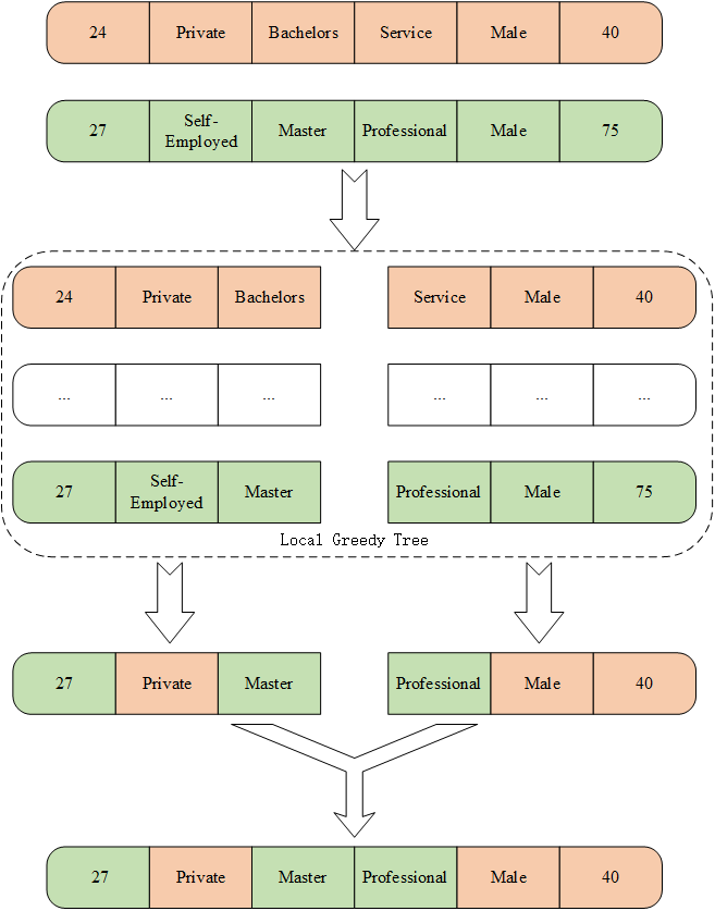
Figure 4: Division and linking of Linking Tree. The division and linking process of the linking tree, the orange feature values indicate the feature values from the query sample, the green feature values indicate the feature values from the prototype case, and the arrows indicate the linking tree division of feature values, local feature value selection, and the feature value filling process.

In Algorithm 2, $\operatorname{calculate}(\cdot)$ indicates the calculation of the score of the combination of local eigenvalues on that path, which can use any of the aforementioned metrics, here rss is used as an example and is calculated as shown in equation (8).

4.4.3 Filling the Feature Space of Counterfactual Explanation

After the first two stages, $k$ sets of local feature selection paths can be obtained, and the process of generating CEs from feature selection paths is shown in Algorithm 3.

Algorithm 3 Filling Counterfactual Explanations.

  

   FILLCE $(P,S,PathList)$

        $path\leftarrow[\ ];$

        $CE\leftarrow[\ ];$

        $\operatorname{for}\ p\operatorname{in}PathList\operatorname{do}:$

            $path\leftarrow path.\operatorname{push}(p);$

            $\operatorname{end}\ \operatorname{for};$

        $\operatorname{for}\ i\leftarrow 1\operatorname{to}\ \operatorname{len}(path)\ do:$

            $\operatorname{if}\ path[i]==0\operatorname{do}:$

                $CE.\operatorname{push}(P[i]);$

            $\operatorname{else}\ \operatorname{do}:$

                $CE.\operatorname{push}(S[i]);$

                $\operatorname{end}\ \operatorname{if};$

            $\operatorname{end}\ \operatorname{for};$

        $\operatorname{return}\ CE;$

The $\operatorname{push}(\cdot)$ operation in Algorithm 3 represents the addition of elements to the specified list, and the $PathList$ represents the $k$ sets of local feature value paths obtained in the previous two steps. The paths are selected by stitching the feature values to control the source of the feature values that are eventually populated into the CE, which in turn is populated by selecting feature values from the prototype case and the query sample.

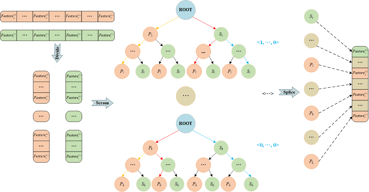
Figure 5: The overall structure of the Linking Tree. The linking tree consists of several local greedy trees, and the root node of each tree stores the path corresponding to the combination of locally optimal features filtered by the previous local greedy tree according to the preset conditions. Finally, all the paths are stitched together and the feature values are selected from the query sample and the prototype case to populate CE according to the complete feature selection path, respectively.

The complete linking tree process is shown in Fig. 5, with the blue dovetail arrows indicating the three processes of the Linking Tree. After dividing the two samples, a number of subsets of local feature values are formed, with the orange and green nodes indicating the features of the prototype case and the query sample respectively. The combination of the local feature values of the two samples is represented by constructing a local greedy tree. The red path is the optimal selection path filtered by the local greedy tree and the grey-green nodes indicating a number of features omitted in between. The final feature values to be filled into the CE feature space can be selected based on the spliced local paths, with the dashed arrows indicating the final feature value filling process. The complete combination of feature values is a CE to be validated, and in order to generate a final valid CE, it needs to rely on the validation model for verification. If the classification result is consistent with the target category, it is considered a valid CE.

4.5 Tree-based Conditions Optional Links

Linking Tree provides a feature-based method for generating CEs. To better accommodate general user preferences, we set up two optional structures and provide several sets of selection methods for each part.

By choosing different prototype cases and setting different feature value selection rules in local greedy trees, different CEs can be generated, and the complete process of T-COL is shown in Fig. 6. If the user prefers more secure and robust CEs, T-COL selects more category-representative samples, i.e. samples of the target category with the highest probability, as prototype cases. In addition, rss will be used as a rule for feature value selection after the construction of local greedy trees. Ultimately T-COL selects one or more combinations of feature values that match the user’s preferences as CEs based on rss, from the set of feature values of the selected prototype cases and the query sample.

4.6 Utilizing T-COL to Address Challenges 3 and 7

According to the previous introduction, T-COL is a feature-based CE generation method with two optional structures. It determines the selection rules for prototype cases and the selection rules for local combinations of feature values based on general user preferences. The prototype cases then lead to the generation of CEs for the query sample based on the linking tree approach.

4.6.1 General user preferences

Capturing user preferences is the main purpose of designing T-COL and is mainly reflected in the two conditional optional structures of T-COL. These two structures are located in key positions in T-COL and allow the inclusion of general user preferences in the generation of CEs.

After establishing a mapping between general user preferences and the different conditions of two structures, the two structures automatically select the conditions that accommodate the user preferences. The first structure controls the selection of prototype cases. In T-COL, the prototype cases are considered ideal cases about user preferences, and CEs are generated by directing the query sample to change toward such cases. The second structure controls the selection of local feature value combinations. It can control the extent to which the query sample changes to the prototype case by controlling which feature values are selected.

In summary, T-COL generates CEs by controlling the query sample to change a certain degree in a certain direction. In which, the direction and degree of change are determined by user preferences. For example, suppose a user wants to focus on a few things, T-COL will select samples with a few feature values different from that of the query sample as the ideal cases. In addition, T-COL selects as few different feature values from the prototype cases as possible during the change.

4.6.2 Variable Machine Learning Systems

There is no structure designed for this problem in T-COL. Robust CEs on variable ML systems are designed to accommodate practical applications where the systems are frequently updated and changed. For this issue, we added $c$ to the general user preferences. General user preference $c$ indicates the desire of users for more robust CEs, with the main issues being variable ML systems and intrusive attacks.

Intrusive attacks are exogenous and need to be addressed in combination with some other means. We focus on solving problems in CE generation, and thus mainly address the generation of more robust CEs on variable ML models. Based on T-COL, we set a set of conditions on general user preferences $c$. We choose the target category samples with the highest classification confidence on the validation model, i.e., the highest classification probability of the validation model, as the prototype cases. In addition, when selecting a combination of local eigenvalues, T-COL encourages the selection of more feature values from the prototype cases. By changing more in the direction of the highest confidence level, more robust CEs can be generated on variable ML systems.

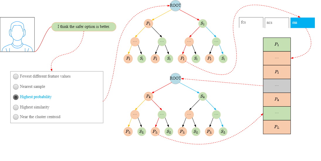
Figure 6: The complete flow of the T-COL, with the red curved dashed lines indicating the flow between the several processes. The user wants a more robust CE, and according to the previous introduction, T-COL first selects the target class sample for which the ML model gives the highest probability as the prototype case. After that, a group of local greedy trees is constructed using the prototype cases and the query sample. For each tree, a combination of local feature values is selected using rss and finally stitched into a CE.

5 Experimental Results

We evaluated the data fidelity of CEs generated by the T-COL method and their adaptability to general user preferences. To assess the adaptability of CEs to user preferences, we also evaluated the proximity, sparsity, validity, and centrality of CEs. The codes, more experimental details, and reappearance methods are available at https://github.com/NEU-DataMining/T-COL.

5.1 Datasets

Referring to the work on CE, we chose the five datasets, the Adult income dataset [46], the German credit dataset [47], the Titanic dataset [48], the Water quality dataset [49], and the Phoneme dataset [50].

• Adult Income. The dataset contains information on population, education, etc. based on the 1994 Census database and is available from the UCI Machine Learning Repository [51]. In this paper, a pre-processed version from [36] was chosen to filter eight of the features. The task of the classification model is to classify whether the individual income of each sample exceeds 50,000 dollars.

• German Credit. The information in this dataset is obtained from banks in relation to personal loans, such as the number of credit cards currently held by a particular bank, the duration of current employment, and other information on a total of 20 characteristics. We use the version obtained directly from the UCI database without processing. The task of the classification model is to determine whether a user is a credit risk or not by determining their credit type based on their attributes.

• Titanic. This dataset is derived from the Titanic incident, in which the gender, age, ticket number, class of ticket, and other attributes of some of the passengers were collected. The dataset contains information about 891 passengers in total, and we removed the instances containing null values. The task of the classification model is to determine whether a passenger will eventually survive.

• Water Quality. This dataset contains water quality measurements and assessments related to potability. Each sample contains nine attributes of one water sample, such as pH, hardness, etc. The dataset contains data for a total of 3276 water instances, and we removed some of the instances that contained null values. The task of the classification model is to discriminate whether a water sample is potable or not.

• Phoneme. The dataset collects five different attributes from 1809 isolated syllables to characterize each vowel. The dataset contains a total of 5404 instances. The task of the classification model is to distinguish between nasal and oral vowels.

Table 3: Validation weights of the third-party model

Model	Adult Income	German Credit	Titanic	Water Quality	Phoneme
KNN	0.73	0.66	0.93	0.62	0.84
MLP	0.75	0.67	0.95	0.64	0.82
SVM	0.74	0.69	0.93	0.62	0.8
DT	0.69	0.65	0.94	0.58	0.83
NB	0.74	0.7	0.93	0.52	0.75

Table 4: The contrasting properties of counterfactual explanations

Datasets	Metrics	Dice-r	Dice-g	Dice-k	T-COL-a	T-COL-b	T-COL-c	T-COL-d	T-COL-e	Spark	Gaps-DiCE	Gaps-Spark
Adult Income	Proximity${}^{(b,d)}\downarrow$	1.07	1.07	1.07	0.96	1.09	1.09	1.07	1.07	0.72	0.11	-0.24
	Sparsity${}^{(a)}\downarrow$	16.75	15.63	14.63	21.25	13.38	19.63	54	57.38	6.5	1.25	-6.88
	Data fidelity${}^{(c)}\uparrow$	0.54	0.74	0.67	0.36	0.45	0.62	0.68	0.7	0.12	-0.04	0.58
	Validity${}^{(c)}\uparrow$	0.6	0.56	0.64	1	1	0.94	0.98	0.98	0	0.36	1
	Centrality${}^{(d,e)}\downarrow$	0.82	0.71	0.7	1.07	0.75	0.63	0.63	0.59	0.96	0.11	0.37
German Credit	Proximity${}^{(b,d)}\downarrow$	0.78	0.78	0.89	0.84	0.65	0.65	0.65	0.65	-	0.13	-
	Sparsity${}^{(a)}\downarrow$	24.3	15.85	16.4	14.75	66.7	82.4	153.15	170.3	-	1.1	-
	Data fidelity${}^{(c)}\uparrow$	0.16	0.79	0.73	0.6	0.72	0.75	0.78	0.8	-	0.01	-
	Validity${}^{(c)}\uparrow$	0.4	0.96	1	0.67	0.91	0.95	1	0.99	-	0	-
	Centrality${}^{(d,e)}\downarrow$	1.05	0.95	1	1.01	0.98	0.94	0.94	0.93	-	0.02	-
Titanic	Proximity${}^{(b,d)}\downarrow$	1.01	1.01	1.15	1.32	1.03	1.03	1.03	1.03	0.89	-0.02	-0.14
	Sparsity${}^{(a)}\downarrow$	23	21	16.33	75.56	149.22	164.33	239.88	252.11	12.44	-59.23	-63.12
	Data fidelity${}^{(c)}\uparrow$	0.92	0.95	0.98	1	0.99	0.99	1	1	0.75	0.02	0.25
	Validity${}^{(c)}\uparrow$	0.96	0.92	0.96	1	1	1	1	1	0.8	0.04	0.2
	Centrality${}^{(d,e)}\downarrow$	0.92	0.92	0.81	0.87	0.83	0.77	0.77	0.76	0.97	0.05	0.21
Water Quality	Proximity${}^{(b,d)}\downarrow$	0.81	0.81	0.89	1.04	0.57	0.57	0.57	0.54	0.99	0.27	0.45
	Sparsity${}^{(a)}\downarrow$	20.44	0	0	3.33	7.89	8.22	11.56	11.78	0	-3.33	-3.33
	Data fidelity${}^{(c)}\uparrow$	0.74	0.47	0.67	0.86	0.76	0.78	0.81	0.81	0.72	0.12	0.14
	Validity${}^{(c)}\uparrow$	0.6	0.88	1	1	0.95	0.97	0.97	0.98	0.65	0	0.35
	Centrality${}^{(d,e)}\downarrow$	0.99	1	0.99	1	0.99	0.99	0.99	0.99	0.99	0	0
Phoneme	Proximity${}^{(b,d)}\downarrow$	0.76	0.76	0.92	1.3	0.54	0.54	0.5	0.5	-	0.26	-
	Sparsity${}^{(a)}\downarrow$	15	0	0	4	8	8	8	8	-	-4	-
	Data fidelity${}^{(c)}\uparrow$	0.56	0.7	0.68	1	0.72	0.77	0.75	0.75	-	0.3	-
	Validity${}^{(c)}\uparrow$	0.68	1	1	1	1	1	1	1	-	0	-
	Centrality${}^{(d,e)}\downarrow$	0.66	0.98	0.98	0.92	0.61	0.61	0.61	0.61	-	0.05	-

Table 5: Counterfactual explanations on preference $c$

Methods	Adult Income	German Credit	Titanic	Water Quality	Phoneme
DiCE	0.7	0.83	0.98	0.75	0.78
T-COL	0.77	0.85	1	0.9	1
Spark	0.09	-	0.76	0.7	-

5.2 Baseline

Three open-source methods for generating CEs are available in DiCE [36] and can provide CEs of high quality on the available evaluation metrics. As a result, DiCE has been used as a baseline for most related studies. We follow the path of these works, again using DiCE as the baseline method. Three methods are provided in DiCE to generate CEs, “genetic”, “random” and “kd-tree”, which we denote as “DiCE-g”, “DiCE-r” and “DiCE-k”, respectively.

In addition, we note that Large Language Models (LLMs) have demonstrated some counterfactual reasoning. As one of the current state-of-the-art in AI, we also consider LLMs as baselines, and Spark was chosen for comparison. However, limited by the coding format of the datasets, we only compared Spark’s performance on the Adult Income, Titanic, and Water Quality datasets.

5.3 Experimental Settings

We randomly selected query samples, coded the target for the categorical features in the samples [52], and generated CEs using T-COL and baseline methods, respectively. In the experiments, we generate five CEs for each query sample. The depth of local greedy trees is set to three.

A random forest model [53] was chosen as the validation model for the CE to verify whether the generated CE was the target class. In addition, common ML models such as decision trees [54] and plain Bayesian [55] were selected as third-party models to evaluate the data veracity of the CEs. The weights of the third-party models were determined using a ten-fold cross-validation [56] approach.

5.4 Adaptability to General User Preferences

To accommodate our pre-defined general user preferences, T-COL provides two optional structures and sets several sets of options during the generation of CEs. We compared the properties of the CEs generated by the T-COL with those of the baseline methods for all combined configurations, and the results are shown in Table 4.

For each sample query, we generated five separate CEs using different methods. Based on the previous theoretical analysis, our proposed feature-based T-COL approach is able to guarantee the feasibility, consistency, data manifold closure, and other properties of the CEs. To evaluate the adaptability of CEs to general user preferences, we evaluated the main properties corresponding to each general user preference.

To facilitate a comparison of the adaptability of CEs to general user preferences, we map each general user preference directly to unique properties. The association between user preferences and the properties of CEs are shown in Table 6.

Table 6: Connections between preferences and properties of CEs

Preferences	Properties
$a$	Sparsity
$b$	Proximity
$c$	Data fidelity, Validity
$d$	Proximity, Centrality
$e$	Centrality

In Table 4, the letter superscripted after each property indicates general user preferences associated with it, the up-arrow indicating better performance for the corresponding larger value and the down-arrow indicating better performance for the smaller value. The “Gaps” indicate the difference between the best results of T-COL and the best results of baseline methods. The CEs generated by T-COL outperformed the baseline approaches in terms of the corresponding properties under different settings. The results show that the T-COL approach is more resilient to general user preferences. Another thing to note is that T-COL does not behave strictly according to our settings regarding user preferences. For example, the CE with the best proximity performance on Adult Income is generated by “T-COL-a” instead of “T-COL-b”.

5.5 Reliability of Counterfactual Explanations

Considering that most users of the application are concerned with the reliability of CEs. We have further analyzed the performance of CEs on preference $c$. The properties associated with the degree of reliability are mainly data fidelity and validity. As a result of ML models are often updated and replaced in the application, we set a higher weight of 0.75 for data fidelity and 0.25 for validity. The weighted average results are shown in Table 5. As can be seen from the table, T-COL can generate more reliable CEs than baseline methods.

5.6 Efficiency Analysis

The efficiency of generating CEs is also very important in applications. During our experiments, we found that the efficiency of DiCE and T-COL in generating CEs differed significantly. Therefore, we analyzed the time complexity of T-COL and DiCE and recorded the actual execution time of the experiment to generate five CEs for each query sample.

5.6.1 Time Complexity Analysis

Define $m$ as the number of CEs generated for each sample, the number of features as $n$, $k$ as the number of samples generated during evaluation, and $T$ as the number of iterations required to optimize the loss function. To facilitate the analysis of the time complexity of T-COL, we define $d$ as the depth of the local greedy tree.

The main time-consuming steps in DiCE’s process of generating CEs are:

• Optimizing the loss function for counterfactual generation.

• Approximating the counterfactual to the decision boundary of the ML model

The execution time of the first step is related to the number of CEs to be generated and the number of iterations. For each CE to be generated, a target loss value can be obtained based on the loss function. DiCE optimizes this loss value by means of an iterative approach, where each iteration requires the calculation of the distance between the query sample and the generated counterfactual sample. The time complexity of this part is $\textsc{O}(T*mn)$. In the second step, a large number of samples need to be generated around the query sample at different distances. In addition, the distance from the query sample to all counterfactual samples needs to be computed. The time complexity of this part is $\textsc{O}(kmn)$. In summary, the time complexity of DiCE is $\textsc{O}((T+k)*mn)$.

The main time-consuming processes of T-COL are mainly the second and third steps, the first step of feature partitioning takes very little time and can be ignored. For the generation of each counterfactual explanation, the second step requires the computation of the values corresponding to the features on all paths of each local greedy tree, with a time complexity related to the depth of the tree and the number of features in the samples as $\textsc{O}(m*\frac{n}{d}*2^{(d-1)})$. The third step requires traversing all the generated counterfactual paths and performing feature selection with a time complexity of $O(mn)$. Note that according to the setup of this paper, $d$ is a constant between three and nine, which gives $1<\frac{1}{d}*2^{(d-1)}<29$, and the time complexity of T-COL can be abbreviated as $\textsc{O}(mn)$.

5.6.2 Runtime Comparison

Based on the previous analysis, the time complexity of T-COL is much smaller than that of DiCE since it does not require a lot of optimization computations. In this section, we list the actual running time of the two methods in our experiments in Table 7, for different datasets.

Table 7: Runtime for generating CEs

Datasets	T-COL-a(s)	T-COL-b	T-COL-c	T-COL-d	T-COL-e	DiCE-r	DiCE-g	DiCE-k
Adult Income	0.3	0.29	0.05	0.27	0.06	0.61	16.19	1.05
German Credit	0.53	0.52	0.1	0.47	0.1	0.85	2.36	19.54
Titanic	0.30	0.29	0.05	0.27	0.06	0.85	2.61	9.36
Water Quality	0.17	0.17	0.03	0.15	0.03	3706.03	0.31	1373.27
Phoneme	0.13	0.13	0.02	0.12	0.02	605.43	0.39	600.4

As shown in Table 7, T-COL generates CEs much more efficiently than DiCE, allowing for real-time response, which is very important in applications. With a local greedy tree depth of 3, T-COL takes less than a second to generate all five CEs for each query sample while “DiCE-r” even takes more than 3,700 seconds to generate five CEs for a sample query in Water Quality.

In our experiments, we found that the generation time difference of T-COL shows a strong correlation with the number of sample features for a fixed local greedy tree depth, which is consistent with the results of our time complexity analysis. In addition, we find that the time required by different optimization methods for DiCE varies significantly in the face of different data types. The “random” method is faster to generate when there are many categorical features while the “genetic” method is faster to generate when there are many numerical features.

6 Conclusion

In this paper, we propose T-COL, a feature value-based method for generating CEs. Our method addresses the problem of user preferences for CEs by providing two optional structures that can adapt to different preferences. To examine the adaptability of CEs to general user preferences, we predefined several sets of possible preferences and established their connection with the properties of CEs. We set different conditions for the optional structures of T-COL to generate CEs that can better adapt to different general user preferences. Furthermore, we conduct further research on generating more robust CEs on variable ML systems. To solve this problem, we incorporate a user preference and establish a group of conditions to guide T-COL in generating robust CEs with higher data fidelity on variable ML systems. Our experiments on five benchmark datasets demonstrate that T-COL better adapts to different user preferences and effectively deals with the problem of variable ML systems. However, we acknowledge that there are still areas for improvement in T-COL. In future work, we plan to expand T-COL by adding general user preferences to accommodate more complex scenarios in real-world applications. Furthermore, we would like to add further constraints on T-COL and enrich its structure to better guarantee the properties of CEs and to address additional issues. In addition, we will further customize the condition settings under each user preference.

Ethical Analysis: The inability of ML models to completely avoid bias during training results in the generation of CEs that may also possess this bias from the validation model. To avoid ethical issues such as bias that may arise from CEs, we selected samples of target categories that do not raise ethical issues as prototype cases.

References

- [1] David Gunning. Explainable artificial intelligence (xai). Defense advanced research projects agency (DARPA), nd Web, 2(2):1, 2017.
- [2] Alejandro Barredo Arrieta, Natalia Díaz-Rodríguez, Javier Del Ser, Adrien Bennetot, Siham Tabik, Alberto Barbado, Salvador García, Sergio Gil-López, Daniel Molina, Richard Benjamins, et al. Explainable artificial intelligence (xai): Concepts, taxonomies, opportunities and challenges toward responsible ai. Information fusion, 58:82–115, 2020.
- [3] David Gunning, Mark Stefik, Jaesik Choi, Timothy Miller, Simone Stumpf, and Guang-Zhong Yang. Xai—explainable artificial intelligence. Science robotics, 4(37):eaay7120, 2019.
- [4] Christoph Molnar. Interpretable machine learning. Lulu. com, 2020.
- [5] Kacper Sokol and Peter A Flach. Counterfactual explanations of machine learning predictions: opportunities and challenges for ai safety. SafeAI@ AAAI, 2019.
- [6] Thao Le, Tim Miller, Ronal Singh, and Liz Sonenberg. Improving model understanding and trust with counterfactual explanations of model confidence. arXiv preprint arXiv:2206.02790, 2022.
- [7] Abubakar Abid, Mert Yuksekgonul, and James Zou. Meaningfully debugging model mistakes using conceptual counterfactual explanations. In Kamalika Chaudhuri, Stefanie Jegelka, Le Song, Csaba Szepesvari, Gang Niu, and Sivan Sabato, editors, Proceedings of the 39th International Conference on Machine Learning, volume 162 of Proceedings of Machine Learning Research, pages 66–88. PMLR, 17–23 Jul 2022.
- [8] S Wachter, BDM Mittelstadt, and C Russell. Counterfactual explanations without opening the black box: automated decisions and the gdpr. Harvard Journal of Law and Technology, 31(2), 2018.
- [9] Ilia Stepin, Jose M Alonso, Alejandro Catala, and Martín Pereira-Fariña. A survey of contrastive and counterfactual explanation generation methods for explainable artificial intelligence. IEEE Access, 9:11974–12001, 2021.
- [10] Riccardo Guidotti. Counterfactual explanations and how to find them: literature review and benchmarking. Data Mining and Knowledge Discovery, pages 1–55, 2022.
- [11] Sahil Verma, John Dickerson, and Keegan Hines. Counterfactual explanations for machine learning: A review. arXiv preprint arXiv:2010.10596, 2020.
- [12] André Artelt and Barbara Hammer. On the computation of counterfactual explanations–a survey. arXiv preprint arXiv:1911.07749, 2019.
- [13] Jürgen Cito, Isil Dillig, Vijayaraghavan Murali, and Satish Chandra. Counterfactual explanations for models of code. In Proceedings of the 44th International Conference on Software Engineering: Software Engineering in Practice, ICSE-SEIP ’22, page 125–134, New York, NY, USA, 2022. Association for Computing Machinery.
- [14] Emanuele Albini, Jason Long, Danial Dervovic, and Daniele Magazzeni. Counterfactual shapley additive explanations. In 2022 ACM Conference on Fairness, Accountability, and Transparency, pages 1054–1070, 2022.
- [15] Yaniv Yacoby, Ben Green, Christopher L Griffin, and Finale Doshi Velez. " if it didn’t happen, why would i change my decision?": How judges respond to counterfactual explanations for the public safety assessment. arXiv preprint arXiv:2205.05424, 2022.
- [16] Andrea Piccione, JW Berkery, SA Sabbagh, and Y Andreopoulos. Predicting resistive wall mode stability in nstx through balanced random forests and counterfactual explanations. Nuclear Fusion, 62(3):036002, 2022.
- [17] Ruoxi Shang, KJ Kevin Feng, and Chirag Shah. Why am i not seeing it? understanding users’ needs for counterfactual explanations in everyday recommendations. In 2022 ACM Conference on Fairness, Accountability, and Transparency, pages 1330–1340, 2022.
- [18] Geemi P Wellawatte, Aditi Seshadri, and Andrew D White. Model agnostic generation of counterfactual explanations for molecules. Chemical science, 13(13):3697–3705, 2022.
- [19] Bevan I Smith, Charles Chimedza, and Jacoba H Bührmann. Individualized help for at-risk students using model-agnostic and counterfactual explanations. Education and Information Technologies, 27(2):1539–1558, 2022.
- [20] Marko Tesic and Ulrike Hahn. Can counterfactual explanations of ai systems’ predictions skew lay users’ causal intuitions about the world? if so, can we correct for that? arXiv preprint arXiv:2205.06241, 2022.
- [21] Riccardo Guidotti, Anna Monreale, Fosca Giannotti, Dino Pedreschi, Salvatore Ruggieri, and Franco Turini. Factual and counterfactual explanations for black box decision making. IEEE Intelligent Systems, 34(6):14–23, 2019.
- [22] Giorgos Filandrianos, Konstantinos Thomas, Edmund Dervakos, and Giorgos Stamou. Conceptual edits as counterfactual explanations. In AAAI Spring Symposium: MAKE, 2022.
- [23] Xinyue Dai, Mark T Keane, Laurence Shalloo, Elodie Ruelle, and Ruth MJ Byrne. Counterfactual explanations for prediction and diagnosis in xai. In Proceedings of the 2022 AAAI/ACM Conference on AI, Ethics, and Society, pages 215–226, 2022.
- [24] Martin Pawelczyk, Chirag Agarwal, Shalmali Joshi, Sohini Upadhyay, and Himabindu Lakkaraju. Exploring counterfactual explanations through the lens of adversarial examples: A theoretical and empirical analysis. In Gustau Camps-Valls, Francisco J. R. Ruiz, and Isabel Valera, editors, Proceedings of The 25th International Conference on Artificial Intelligence and Statistics, volume 151 of Proceedings of Machine Learning Research, pages 4574–4594. PMLR, 28–30 Mar 2022.
- [25] Greta Warren, Mark T Keane, and Ruth MJ Byrne. Features of explainability: How users understand counterfactual and causal explanations for categorical and continuous features in xai. arXiv preprint arXiv:2204.10152, 2022.
- [26] Ulrike Kuhl, André Artelt, and Barbara Hammer. Let’s go to the alien zoo: Introducing an experimental framework to study usability of counterfactual explanations for machine learning. arXiv preprint arXiv:2205.03398, 2022.
- [27] Dylan Slack, Anna Hilgard, Himabindu Lakkaraju, and Sameer Singh. Counterfactual explanations can be manipulated. In M. Ranzato, A. Beygelzimer, Y. Dauphin, P.S. Liang, and J. Wortman Vaughan, editors, Advances in Neural Information Processing Systems, volume 34, pages 62–75. Curran Associates, Inc., 2021.
- [28] André Artelt, Valerie Vaquet, Riza Velioglu, Fabian Hinder, Johannes Brinkrolf, Malte Schilling, and Barbara Hammer. Evaluating robustness of counterfactual explanations. In 2021 IEEE Symposium Series on Computational Intelligence (SSCI), pages 01–09. IEEE, 2021.
- [29] Marco Virgolin and Saverio Fracaros. On the robustness of counterfactual explanations to adverse perturbations. arXiv preprint arXiv:2201.09051, 2022.
- [30] Sahil Verma, John Dickerson, and Keegan Hines. Counterfactual explanations for machine learning: Challenges revisited. arXiv preprint arXiv:2106.07756, 2021.
- [31] Peyman Rasouli and Ingrid Chieh Yu. Care: Coherent actionable recourse based on sound counterfactual explanations. International Journal of Data Science and Analytics, pages 1–26, 2022.
- [32] Furui Cheng, Yao Ming, and Huamin Qu. Dece: Decision explorer with counterfactual explanations for machine learning models. IEEE Transactions on Visualization and Computer Graphics, 27(2):1438–1447, 2021.
- [33] Diederik P Kingma and Jimmy Ba. Adam: A method for stochastic optimization. arXiv preprint arXiv:1412.6980, 2014.
- [34] Donato Maragno, Tabea E Röber, and Ilker Birbil. Counterfactual explanations using optimization with constraint learning. arXiv preprint arXiv:2209.10997, 2022.
- [35] Berk Ustun, Alexander Spangher, and Yang Liu. Actionable recourse in linear classification. In Proceedings of the conference on fairness, accountability, and transparency, pages 10–19, 2019.
- [36] Ramaravind K Mothilal, Amit Sharma, and Chenhao Tan. Explaining machine learning classifiers through diverse counterfactual explanations. In Proceedings of the 2020 conference on fairness, accountability, and transparency, pages 607–617, 2020.
- [37] Pau Rodríguez, Massimo Caccia, Alexandre Lacoste, Lee Zamparo, Issam Laradji, Laurent Charlin, and David Vazquez. Beyond trivial counterfactual explanations with diverse valuable explanations. In Proceedings of the IEEE/CVF International Conference on Computer Vision (ICCV), pages 1056–1065, October 2021.
- [38] Khanh Hiep Tran, Azin Ghazimatin, and Rishiraj Saha Roy. Counterfactual explanations for neural recommenders. In Proceedings of the 44th International ACM SIGIR Conference on Research and Development in Information Retrieval, pages 1627–1631, 2021.
- [39] Stratis Tsirtsis and Manuel Gomez Rodriguez. Decisions, counterfactual explanations and strategic behavior. Advances in Neural Information Processing Systems, 33:16749–16760, 2020.
- [40] Mark T Keane and Barry Smyth. Good counterfactuals and where to find them: A case-based technique for generating counterfactuals for explainable ai (xai). In International Conference on Case-Based Reasoning, pages 163–178. Springer, 2020.
- [41] Barry Smyth and Mark T Keane. A few good counterfactuals: generating interpretable, plausible and diverse counterfactual explanations. In International Conference on Case-Based Reasoning, pages 18–32. Springer, 2022.
- [42] Yash Goyal, Ziyan Wu, Jan Ernst, Dhruv Batra, Devi Parikh, and Stefan Lee. Counterfactual visual explanations. In International Conference on Machine Learning, pages 2376–2384. PMLR, 2019.
- [43] André Artelt, Valerie Vaquet, Riza Velioglu, Fabian Hinder, Johannes Brinkrolf, Malte Schilling, and Barbara Hammer. Evaluating robustness of counterfactual explanations. In 2021 IEEE Symposium Series on Computational Intelligence (SSCI), pages 01–09, 2021.
- [44] Thibault Laugel, Marie-Jeanne Lesot, Christophe Marsala, and Marcin Detyniecki. Issues with post-hoc counterfactual explanations: a discussion. arXiv preprint arXiv:1906.04774, 2019.
- [45] Mark T Keane, Eoin M Kenny, Eoin Delaney, and Barry Smyth. If only we had better counterfactual explanations: Five key deficits to rectify in the evaluation of counterfactual xai techniques. arXiv preprint arXiv:2103.01035, 2021.
- [46] Ron Kohavi et al. Scaling up the accuracy of naive-bayes classifiers: A decision-tree hybrid. In Kdd, volume 96, pages 202–207, 1996.
- [47] Jeroen Eggermont, Joost N Kok, and Walter A Kosters. Genetic programming for data classification: Partitioning the search space. In Proceedings of the 2004 ACM symposium on Applied computing, pages 1001–1005, 2004.
- [48] Will Cukierski. Titanic - machine learning from disaster, 2012.
- [49] Laksika Tharmalingam. Water quality and potability, 2023.
- [50] Rafael Gomes Mantovani. phoneme, 2015.
- [51] Dheeru Dua and Casey Graff. UCI machine learning repository, 2017.
- [52] Daniele Micci-Barreca. A preprocessing scheme for high-cardinality categorical attributes in classification and prediction problems. ACM SIGKDD Explorations Newsletter, 3(1):27–32, 2001.
- [53] Gérard Biau and Erwan Scornet. A random forest guided tour. Test, 25(2):197–227, 2016.
- [54] S Rasoul Safavian and David Landgrebe. A survey of decision tree classifier methodology. IEEE transactions on systems, man, and cybernetics, 21(3):660–674, 1991.
- [55] Irina Rish et al. An empirical study of the naive bayes classifier. In IJCAI 2001 workshop on empirical methods in artificial intelligence, volume 3, pages 41–46, 2001.
- [56] Payam Refaeilzadeh, Lei Tang, and Huan Liu. Cross-validation. Encyclopedia of database systems, 5:532–538, 2009.