$t\geq 1$

Differentially Private Secure Multiplication: Hiding Information in the Rubble of Noise

Abstract

We consider the problem of private distributed multi-party multiplication. It is well-established that Shamir secret-sharing coding strategies can enable perfect information-theoretic privacy in distributed computation via the celebrated algorithm of Ben Or, Goldwasser and Wigderson (the “BGW algorithm”). However, perfect privacy and accuracy require an honest majority, that is, $N\geq 2t+1$ compute nodes are required to ensure privacy against any $t$ colluding adversarial nodes. By allowing for some controlled amount of information leakage and approximate multiplication instead of exact multiplication, we study coding schemes for the setting where the number of honest nodes can be a minority, that is $N<2t+1.$ We develop a tight characterization privacy-accuracy trade-off for cases where $N<2t+1$ by measuring information leakage using differential privacy instead of perfect privacy, and using the mean squared error metric for accuracy. A particularly novel technical aspect is an intricately layered noise distribution that merges ideas from differential privacy and Shamir secret-sharing at different layers.

1 Introduction

Ensuring privacy in distributed data processing is a central engineering challenge in modern machine learning. Two common privacy definitions in data processing are information-theoretic (perfect) privacy and differential privacy [1, 2]. Perfect information-theoretic privacy is the most stringent definition, requiring that no private information is revealed to colluding adversary nodes regardless of their computational resources. Differential privacy, in turn, allows a tunable level of privacy and ensures that an adversary cannot distinguish inputs that differ by a small perturbation (i.e., “neighboring” inputs).

Coding strategies have a decades-long history of enabling perfect information-theoretic privacy in distributed computing. The most celebrated is the BGW algorithm [3, 4], which ensures information-theoretically private distributed computations for a wide class of functions. The BGW algorithm adapts Shamir secret-sharing [5] — a technique that uses Reed-Solomon codes for distributed data storage with privacy constraints — to multiparty function computation. Consider two random variables ${A},{B}\in\mathbb{F},$ where $\mathbb{F}$ is a field, and a set of $N$ computation nodes. Let ${R}_{i},{S}_{i}\in\mathbb{F},i=1,2,\ldots,t$ be statistically independent random variables. In Shamir’s secret sharing, node $i$ receives inputs $\tilde{{A}}_{i}=p_{1}(x_{i}),\tilde{{B}}_{i}=p_{2}(x_{i}),$ where, $x_{1},x_{2},\ldots,x_{N}\in\mathbb{F}$ are distinct non-zero scalars and $p_{1}(x),p_{2}(x)$ are polynomials:

$$p_{1}(x)={A}+\sum_{j=1}^{t}{R}_{j}x^{j},p_{2}(x)={B}+\sum_{i=1}^{t}{S}_{j}x^{j}.$$

If the field $\mathbb{F}$ is finite and ${R}_{i},{S}_{i},i=1,2,\ldots,t$ are uniformly distributed over the field elements, then the input to any subset $\mathcal{S}$ of $t$ nodes is independent of the data $({A},{B}).$ The Shamir secret-sharing coding scheme allows the BGW algorithm to recover any linear combination of the inputs from any subset of $t+1$ nodes. To obtain $\alpha A+\beta B$ for fixed constants $\alpha,\beta\in\mathbb{F},$ node $i$ computes $\alpha\tilde{{A}}_{i}+\beta{{B}}_{i}$ for $\alpha,\beta\in\mathbb{F}.$ The sum $\alpha{A}+\beta{B}$ — which is the constant in the polynomial $\alpha p_{1}(x)+\beta p_{2}(x)$ — can be recovered from the computation output of any $t+1$ of the $N$ nodes by polynomial interpolation. Observe, similarly, that $\tilde{{A}}_{i}\tilde{{B}}_{i}$ can be interpreted as an evaluation at $x=x_{i}$ of the degree $2t$ polynomial $p_{1}(x)p_{2}(x),$ whose constant term is ${A}{B}$. Thus, the product ${A}{B}$ can be recovered from any $2t+1$ nodes via polynomial interpolation (See Fig. 1 (a)). The BGW algorithm uses Shamir secret-sharing to perform secure MPC for the universal class of computations that can be expressed as sums and products while maintaining (perfect) data privacy. However, notice that perfect privacy comes at an infrastructural overhead for non-linear computations. When computing the product, the BGW algorithm requires an “honest majority”, that is, it requires $N\geq 2t+1$ computing nodes in order to ensure privacy against any $t$ colluding nodes. In contrast, only $t+1$ nodes are required for linear computations. This overhead becomes prohibitive for more complex functions, leading to multiple communication rounds or additional redundant computing nodes (see, for example, [3, 6]).

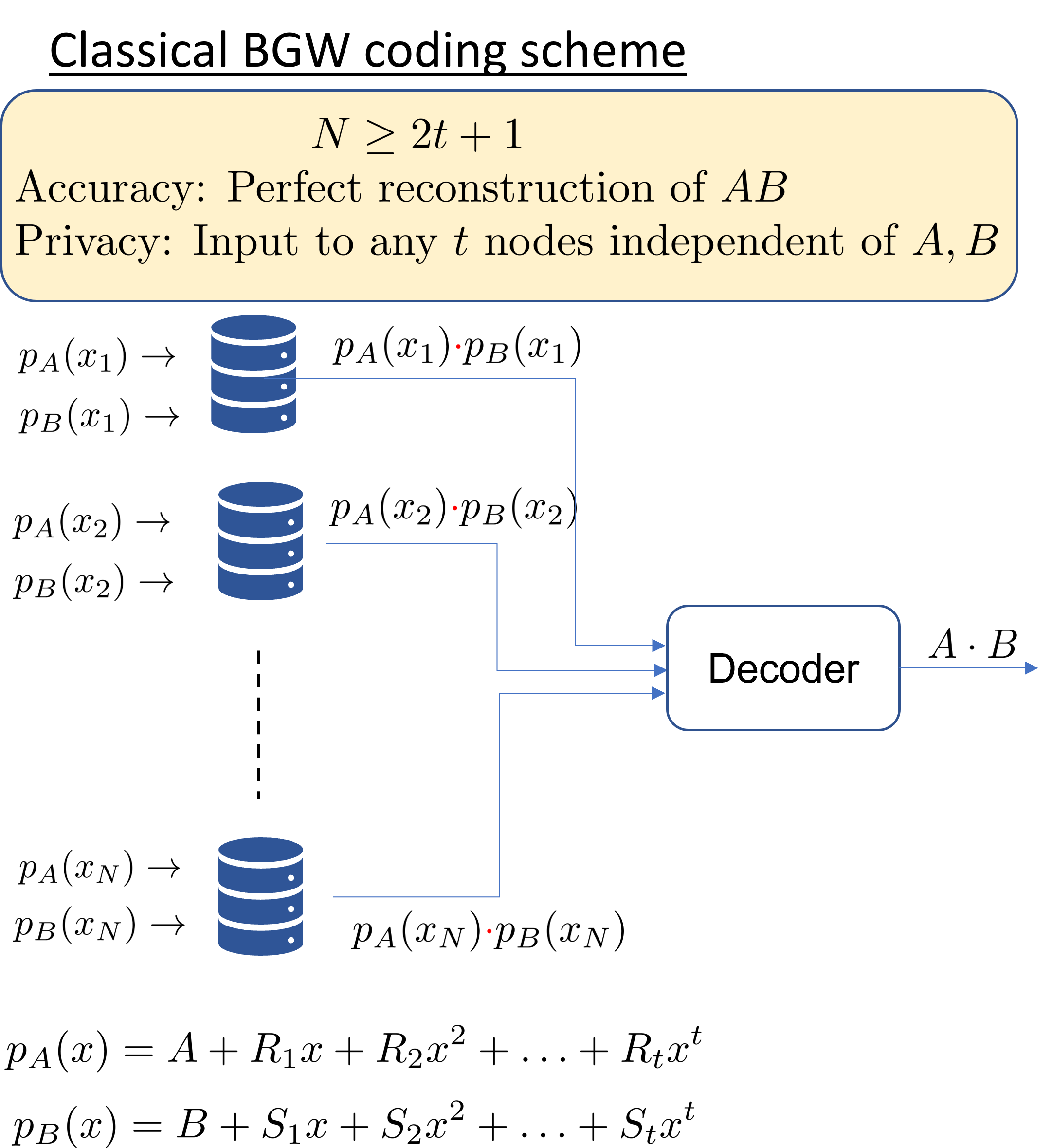
(a) The Shamir secret-sharing coding scheme used in the BGW algorithm.

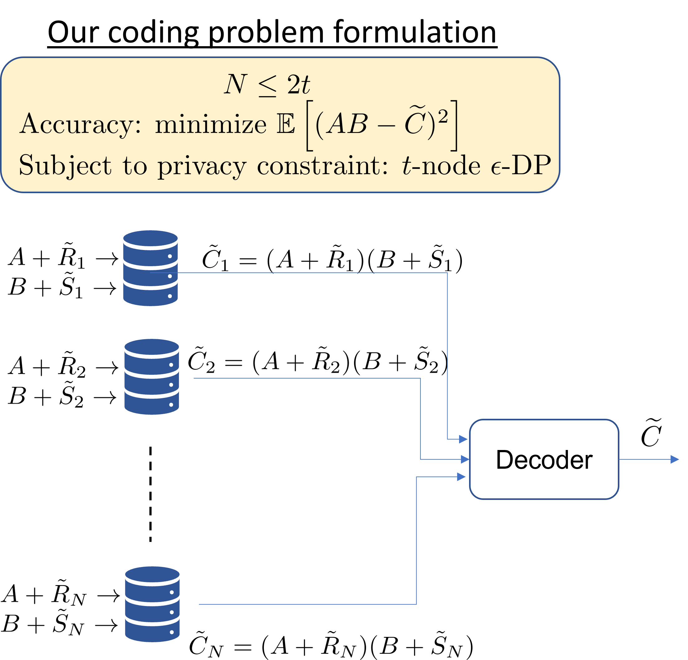
(b) Privacy-Accuracy Trade-off for $N<2t+1$. The privacy requirement is that the input to every subset of $t$ nodes must satisfy $\epsilon$ differential privacy.

Figure 1: Pictorial depiction of our problem formulation and comparison with the coding scheme used in the BGW algorithm.

In this paper, we study the problem of secure multiplication for real-valued data and explore coding schemes that enable a set of fewer than $2t+1$ nodes to compute the product while keeping the data private from any $t$ nodes. While exact recovery of the product and perfect privacy is simultaneously impossible, we propose a novel coding formulation that allows for approximations on both fronts, enabling an accuracy-privacy trade-off analysis. Our formulation utilizes differential privacy (DP) — the standard privacy metric to quantify information leakage when perfect privacy cannot be guaranteed[7]. It is worth noting that approximate computation suffices for several applications, particularly in machine learning, where both training algorithms and inference outcomes are often stochastic. Also, notably, DP is a prevalent paradigm for data privacy in machine learning applications in practice (e.g., [8, 9]).

For single-user computation, where a user queries a database in order to compute a desired function over sensitive data, differential privacy can be ensured by adding noise to the computation output [1]. The study of optimal noise distributions for privacy-utility trade-offs in the release of databases for computation of specific classes of functions is an active area of research in differential privacy literature [7, 10, 11, 12]. Our contribution is the discovery of optimal noise structures for multiplication in the multi-user setting, where the differential privacy constraints are on a set of $t$ colluding adversaries.

Summary of Main Results

We consider a computation system with $N$ nodes where each node receives noisy versions of inputs $A,B$ and computes their product (See Fig. 1(b)). The goal of the decoder is to recover an estimate ${\widetilde{C}}$ of the product ${A}{B}$ from $N$ computation outputs at a certain accuracy level, measured in terms of the mean squared error. The noise distribution should ensure that the input to any subset of $t$ nodes in the system satisfies $\epsilon$-differential privacy (abbreviated henceforth as $t$-node $\epsilon$-DP). Given $N,t$ and the DP parameter $\epsilon,$ our main result provides a tight expression for the minimum possible mean squared error at the decoder for any $N\geq t$. Of particular importance is our result for the regime $t<N<2t+1.$ While our results provide a characterization in terms of differential privacy, they yield an intuitive description when presented in terms of signal-to-noise ratio (SNR) metrics for both privacy and accuracy. Privacy SNR ($\text{SNR}_{p}$) describes how well $t$ colluding nodes can extract the private inputs $A$, $B$, i.e., higher privacy SNR means poor privacy. Accuracy SNR ($\text{SNR}_{a}$) shows how well $N$ nodes can recover the computation output $AB$. Through a non-trivial converse argument, we show that for any $N<2t+1$:

$$(1+\text{SNR}_{a})\leq(1+\text{SNR}_{p})^{2}.$$ (1.1)

We provide an achievable scheme that meets the converse bound arbitrarily closely for $N\geq t+1$. Surprisingly, (1.1) does not depend on $t,N$ — the trade-off remains the same for $N\in\{t+1,t+2,\ldots 2t\}.$ Thus, our main result implies that for the regime of $t<N<2t+1$, remarkably, having more computation nodes does not lead to increased accuracy.

The main technical contribution of our paper is the development of an intricate noise distribution that achieves the optimal trade-off. On the one hand, the Shamir secret-sharing coding scheme used in BGW operates over a finite field, and relies on linear combinations of independent noise variables to achieve perfect secrecy; the connection to coding theory comes from certain rank requirements for these linear combinations. On the other hand, single-user differential privacy schemes typically control the magnitude of the noise to prevent data reconstruction up to a distortion (sensitivity) level whilst revealing sufficient information to enable accurate computations. Our optimal noise distribution has a layered structure and utilizes these different approaches in different layers.

In our achievable scheme, each node gets a superposition of three random variables, e.g., node $i$ gets $A+Y_{1}^{(i)}+Y_{2}^{(i)}+Y_{3}^{(i)}.$ The three random variables $Y_{1},Y_{2},Y_{3}$ can be interpreted as occurring in three layers. Noise variable $Y_{1}$ controls the magnitude of the noise and is designed to achieve $\epsilon$-DP for a single input. Noise variable $Y_{3}$ is correlated with $Y_{1}$ and enables a legitimate decoder with access to all $N$ nodes to improve the accuracy. The noise variables $Y_{2}^{(i)},i=1,2,\ldots,N$ are designed to ensure $\epsilon$-DP against a colluding adversary. Specifically, they are designed similarly to Shamir secret-sharing to guarantee linear independence constraints that block a colluding adversary from obtaining $Y_{3}$. The magnitudes of the noise variables $Y_{1},Y_{2},Y_{3}$ are designed to satisfy several relations that are surprising at first sight. Specifically, our achievable scheme has the characteristic that $\text{SNR}_{a}$ approaches the converse (1.1) if $\frac{\texttt{var}(Y_{2})}{\texttt{var}(Y_{1})}\rightarrow 0$ and $\frac{\texttt{var}(Y_{3})}{\texttt{var}(Y_{2})}\rightarrow 0$, in addition to other limit relations. For a single user, say node $i$, the noise variables $Y_{2}^{(i)},Y_{3}^{(i)}$ have a negligible effect on its input. In the multi-user scenario that we are considering, a decoder or an adversary can have access to the outputs of multiple nodes. If the variables $Y_{1}(i),i=1,2,\ldots,N$ are sufficiently correlated, the node can peel the first layer of noise, and both $Y_{2},Y_{3}$ then can play a non-negligible role in the residue. Indeed, our noise variables $Y_{2}$ are designed to ensure that a set of $t$ colluding adversaries cannot get access to third layer $Y_{3},$ whereas a legitimate decoder that accesses $t+1$ nodes can peel the second layer $Y_{2}$ and utilize the effect of $Y_{3}$ to reduce the effect of the overall noise and improve the accuracy. Because our achievable scheme requires the summation of noise random variables whose variances are infinitesimally negligible compared to the data magnitude, implementing our scheme in practice requires high precision. In Section 6, we analyze the precision requirements of our achievable scheme.

1.1 Related Work

Differential Privacy and Secure MPC: Several prior works are motivated like us to reduce computation and communication overheads of secure MPC by connecting it with the less stringent privacy guarantee offered by DP. References [13, 14, 15, 16, 17, 18, 19] provide methods to reduce communication overheads and improve robustness while guaranteeing differential privacy for sample aggregation algorithms, label private training, record linkage and distributed median computation. In comparison we aim to develop and study coding schemes with optimal privacy-accuracy trade-offs for differentially private distributed multiplication that reduce the overhead of $t$ redundant nodes.

Coded Computing: The emerging area of coded computing enables the study of codes for secure computing that enable data privacy. Our framework resonates with the coded computing approach, as we abstract the algorithmic/protocol related aspects into a master node, and highlight the role of the error correcting code in our model. Coded computing has been applied to study code design for secure multiparty computing in [20, 21, 22, 23, 24, 25, 26]. These references effectively extend the standard BGW setup by imposing memory constraints on the nodes, or other constraints, that effectively disable each node storing information equivalent to the entire data sets. Under the imposed constraints, these references develop novel codes for exact computation and perfect privacy. In particular, codes for secure MPC over real-valued fields have been studied in [27, 21] extending the ideas of [20] to understand the loss of accuracy due to finite precision. In particular, reference [21] casts the effect of finite precision in a privacy-accuracy tradeoff framework. In contrast to all previous works in coded computing geared towards secure MPC, we operate below the threshold of perfect recovery and characterize privacy-accuracy trade-offs. Our incorporation of differential privacy for this characterization is a novel aspect of our set up. We do not impose any memory constraints on the nodes, and imposition of such constraints can lead to interesting areas of future study.

Privacy-Utility Trade-offs. There is a fundamental trade-off between DP and utility (see [10, 11, 12] for examples in machine learning and statistics). The optimal $\epsilon$-DP noise-adding mechanism for a target moment constraint on the additive noise was characterized in [28]. For approximate DP, near-optimal additive noise mechanisms under $\ell_{1}$-norm and variance constraints were recently given in [29].

2 System Model and Statement of Main Results

We present our system model for distributed differentially private multiplication and state our main results. Our model and results are presented for the case of scalar multiplication here. Natural extensions of the results for the case of matrix multiplication is presented in Sec. 5.

2.1 System Model

We consider a computation system with $N$ computation nodes. ${A},{B}\in\mathbb{R}$ are random variables, and node $i\in\{1,2,\ldots,N\}$ receives:

$$\tilde{{A}}_{i}=a_{i}{A}+\tilde{R}_{i},~{}~{}~{}\tilde{{B}}_{i}=b_{i}{B}+\tilde{S}_{i},$$ (2.2)

where $\tilde{R}_{i},\tilde{S}_{i}\in\mathbb{R}$ are random variables such that $(\tilde{R}_{1},\tilde{R}_{2},\ldots,\tilde{R}_{N},\tilde{S}_{1},\tilde{S}_{2},\ldots,\tilde{S}_{N})$ is statistically independent of $({A},{B}),$ and $a_{i},b_{i}\in\mathbb{R}$ are constants. In this paper, we assume no shared randomness between $(\tilde{R}_{1},\tilde{R}_{2},\ldots,\tilde{R}_{N})$ and $(\tilde{S}_{1},\tilde{S}_{2},\ldots,\tilde{S}_{N})$ i.e., they are statistically independent: $\mathbb{P}_{\tilde{R}_{1},\tilde{R}_{2},\ldots,\tilde{R}_{N},\tilde{S}_{1},\tilde{S}_{2},\ldots,\tilde{S}_{N}}=\mathbb{P}_{\tilde{R}_{1},\tilde{R}_{2},\ldots,\tilde{R}_{N}}\mathbb{P}_{\tilde{S}_{1},\tilde{S}_{2},\ldots,\tilde{S}_{N}}$. For $i\in\{1,2,\ldots,N\},$ computation node $i$ outputs:

$${\tilde{C}}_{i}=\tilde{{A}}_{i}\tilde{{B}}_{i}.$$ (2.3)

A decoder receives the computation output from all $N$ nodes and performs a map: $d:\mathbb{R}^{N}\rightarrow\mathbb{R}$ that is affine over $\mathbb{R}.$ That is, the decoder produces:

$${\widetilde{C}}=d(\tilde{{C}}_{1},\dots,\tilde{C}_{N})=\sum_{i=1}^{N}w_{i}\tilde{{C}}_{i}+w_{0},$$ (2.4)

where the coefficients $w_{i}\in\mathbb{R},$ specify the linear map $d$.

A $N$-node secure multiplication coding scheme consists of the joint distributions of $(\tilde{R}_{1},\tilde{R}_{2},\ldots,\tilde{R}_{N})$ and $(\tilde{S}_{1},\tilde{S}_{2},\ldots,\tilde{S}_{N}),$ scalars $a_{1},a_{2},\ldots,a_{N},b_{1},b_{2},\ldots,b_{N}$ and the decoding map ${d}:\mathbb{R}^{N}\rightarrow\mathbb{R}.$ The performance of a secure multiplication coding scheme is measured in its differential privacy parameters and its accuracy, defined next.

Definition 2.1.

($t$-node $\epsilon$-DP) Let $\epsilon\geq 0$. A coding scheme with random noise variables

$$(\tilde{R}_{1},\tilde{R}_{2},\ldots,\tilde{R}_{N}),(\tilde{S}_{1},\tilde{S}_{2},\ldots,\tilde{S}_{N})$$

and scalars $a_{i},b_{i}\;(i\in\{1,\ldots,N\})$ satisfies $t$-node $\epsilon$-DP if, for any ${A}_{0},{B}_{0},{A}_{1},{B}_{1}\in\mathbb{R}$ that satisfy $\left|\left|\begin{bmatrix}{A}_{0}\\ {B}_{0}\end{bmatrix}-\begin{bmatrix}{A}_{1}\\ {B}_{1}\end{bmatrix}\right|\right|_{\infty}\leq 1$,

$$\max\left(\frac{\mathbb{P}\left(\mathbf{Z}^{(0)}_{\mathcal{T}}\in\mathcal{A}\right)}{\mathbb{P}\left(\mathbf{Z}^{(1)}_{\mathcal{T}}\in\mathcal{A}\right)},\frac{\mathbb{P}\left(\mathbf{Y}^{(0)}_{\mathcal{T}}\in\mathcal{A}\right)}{\mathbb{P}\left(\mathbf{Y}^{(1)}_{\mathcal{T}}\in\mathcal{A}\right)}\right) \leq e^{\epsilon}$$ (2.5)

for all subsets $\mathcal{T}\subseteq\{1,2,\ldots,N\},|\mathcal{T}|=t$, for all subsets $\mathcal{A}\subset\mathbb{R}^{1\times t}$ in the Borel $\sigma$-field, where, for $\ell=0,1$,

$$\mathbf{Y}_{\mathcal{T}}^{(\ell)} \triangleq \begin{bmatrix}a_{i_{1}}{A}_{\ell}+\tilde{R}_{i_{1}}&a_{i_{2}}{A}_{\ell}+\tilde{R}_{i_{2}}&\ldots&a_{i_{|\mathcal{T}|}}{A}_{\ell}+\tilde{R}_{i_{|\mathcal{T}|}}\end{bmatrix}$$ (2.6)

$$\mathbf{Z}_{\mathcal{T}}^{(\ell)} \triangleq \begin{bmatrix}b_{i_{1}}{B}_{\ell}+\tilde{S}_{i_{1}}&b_{i_{2}}{B}_{\ell}+\tilde{S}_{i_{2}}&\ldots&b_{i_{|\mathcal{T}|}}{B}_{\ell}+\tilde{S}_{i_{|\mathcal{T}|}}\end{bmatrix},$$ (2.7)

where $\mathcal{T}=\{i_{1},i_{2},\ldots,i_{|\mathcal{T}|}\}.$

While privacy guarantees must make minimal assumptions on the data distribution, it is common to make assumptions on the data distribution and its parameters when quantifying utility guarantees (e.g., accuracy) [30, 31, 21, 25]. We next state the conditions under which our accuracy guarantees hold.

Assumption 2.1.

${A}$ and ${B}$ are statistically independent random variables that satisfy

$$\mathbb{E}\left[{A}^{2}\right],\mathbb{E}\left[{B}^{2}\right]{\leq\eta}$$

for a parameter $\eta>0$.

It is worth noting that the above assumption implies that $\mathbb{E}[A^{2}B^{2}]\leq\eta^{2}.$ We measure the accuracy of a coding scheme via the mean square error of the decoded output with respect to the product $AB$. Specifically, we define:

Definition 2.2 (Linear Mean Square Error (LMSE)).

For a secure multiplication coding scheme $\mathcal{C}$ consisting of joint distribution $\mathbb{P}_{\tilde{R}_{1},\tilde{R}_{2},\ldots,\tilde{R}_{N},\tilde{S}_{1},\tilde{S}_{2},\ldots,\tilde{S}_{N}},$ decoding map $d:\mathbb{R}^{N}\rightarrow\mathbb{R}$, the LMSE is defined as:

$$\texttt{LMSE}(\mathcal{C})=\mathbb{E}[|{AB}-\widetilde{C}|^{2}].$$ (2.8)

where $\widetilde{{C}}$ is defined in (2.4).

The expectation in the above definition is over the joint distributions of the random variables ${A},{B},\tilde{R_{i}}|_{i=1}^{N},\tilde{S_{i}}|_{i=1}^{N}$. For fixed parameters, $N,t,\epsilon,\eta$, the goal of this paper is to characterize:

$$\inf_{\mathcal{C}}\sup_{\mathbb{P}_{A,B}}\texttt{LMSE}(\mathcal{C})$$

where the infimum is over the set of all coding schemes $\mathcal{C}$ that satisfy $t$-node $\epsilon$-DP, and the supremum is over all distributions $\mathbb{P}_{A,B}$ that satisfy Assumption 2.1.

In the remainder of this paper, we make the following zero mean assumptions: we assume that that $\mathbb{E}(A)=\mathbb{E}(B)=0$ and that $\mathbb{E}[\tilde{R}_{i}]=\mathbb{E}[\tilde{S}_{i}]=0,\forall i\in\{1,2,\ldots,N\}.$ With these assumptions, it suffices to assume that decoder is linear (that is, it is not just affine), since the optimal affine decoders are in fact linear. The reader may readily verify that our results hold without the zero-mean assumptions with affine decoders.

2.2 Signal-to-Noise Ratios

We take a two-step technical approach. First, we characterize accuracy-privacy trade-off in terms of signal-to-noise ratio (SNR) metrics (defined below). Second, we obtain the trade-off between mean square error and differential privacy parameters as corollaries to the SNR trade-off.

We define two SNR metrics: the privacy SNR and the accuracy SNR.

Definition 2.3.

(Privacy signal to noise ratio.) Consider a secure multiplication coding scheme $\mathcal{C}.$ For any set $\mathcal{S}=\{s_{1},s_{2},\ldots,s_{|\mathcal{S}|}\}\subseteq\{1,2,\ldots,N\}$ of nodes where $s_{1}<s_{2}<\ldots<s_{|\mathcal{S}|}$, let $\mathbf{K}_{\mathcal{S}}^{\mathbf{R}}$ and $\mathbf{K}_{\mathcal{S}}^{\mathbf{S}}$ represent the covariance matrices of $\tilde{R}_{i}|_{i\in\mathcal{S}},\tilde{S}_{i}|_{i\in\mathcal{S}}.$ In particular, the $(i,j)$-th entry of $\mathbf{K}_{\mathcal{S}}^{\mathbf{R}},\mathbf{K}_{\mathcal{S}}^{\mathbf{S}}$ are $\mathbb{E}[\tilde{R}_{s_{i}}\tilde{R}_{s_{j}}],\mathbb{E}[\tilde{S}_{s_{i}}\tilde{S}_{s_{j}}]$ respectively. Let $\mathbf{K}_{\mathcal{S}}^{A},t\mathbf{K}_{\mathcal{S}}^{B}$ denote the matrices whose $(i,j)$-th entries respectively are $a_{s_{i}}a_{s_{j}}\eta^{2}$ and $b_{s_{i}}b_{s_{j}}\eta^{2}$ where $a_{i},b_{i}$ are constants defined in (2.2). Then, the privacy signal-to-noise ratios corresponding to inputs ${A},{B}$ denoted respectively as $\texttt{SNR}_{\mathcal{S}}^{A},\texttt{SNR}_{\mathcal{S}}^{B}$ are defined as:

$$\texttt{SNR}_{\mathcal{S}}^{A}=\frac{\text{det}(\mathbf{K}_{\mathcal{S}}^{A}+\mathbf{K}_{\mathcal{S}}^{{R}})}{\text{det}(\mathbf{K}_{\mathcal{S}}^{{R}})}-1,$$

$$\texttt{SNR}_{\mathcal{S}}^{B}=\frac{\text{det}(\mathbf{K}_{\mathcal{S}}^{B}+\mathbf{K}_{\mathcal{S}}^{\mathbf{S}})}{\text{det}(\mathbf{K}_{\mathcal{S}}^{\mathbf{S}})}-1,$$

where ‘det’ denotes the determinant. For $t\leq N$, the $t$-node privacy signal-to-noise ratio of a $N$-node secure multiplication coding scheme $\mathcal{C}$, denoted as $\texttt{SNR}_{p}(\mathcal{C})$ is defined to be:

$$\texttt{SNR}_{p}(\mathcal{C})=\max_{\mathcal{S}\subseteq\{1,2,\ldots,N\},|\mathcal{S}|=t}\max(\texttt{SNR}_{\mathcal{S}}^{A},\texttt{SNR}_{\mathcal{S}}^{B}).$$

Remark 1.

Standard linear mean square estimation theory dictates that a colluding adversary with access to nodes in $\mathcal{S}$ can obtain a linear combination of the inputs to these nodes to recover, for example, $A$ with a mean square error of $\frac{\eta}{1+\texttt{SNR}_{\mathcal{S}}^{\mathcal{A}}}$ (see, for example, equation (13) in [32]). This mean square error is an alternate metric — as compared to DP — for privacy leakage that will be used as an intermediate step in deriving our results.We later convert SNR guarantees into $\epsilon$-DP guarantees.

Next we define the accuracy signal-to-noise ratios. From the definition of $\tilde{C}_{i}$ in (2.3), we observe that:

$$\widetilde{C}_{i}=a_{i}b_{i}AB+a_{i}A\tilde{S}_{i}+b_{i}B\tilde{R}_{i}+\tilde{R}_{i}\tilde{S}_{i}.$$

To understand the following definition, it helps to note that in $\mathbb{E}[\widetilde{C}_{i}\widetilde{C}_{j}]$, the “signal” component, $\mathbb{E}[AB]$, has the coefficient $a_{i}b_{i}a_{j}b_{j}$.

Definition 2.4.

(Accuracy signal to noise ratio.) Consider a secure multiplication coding scheme $\mathcal{C}$ over $N$ nodes. Let $\mathbf{K}_{1}$ denote the $N\times N$ matrix whose $(i,j)$-th entry is $\mathbb{E}[\tilde{C}_{i}\tilde{C}_{j}]$ where $\tilde{C}_{i},\tilde{C}_{j}$ are as defined in (2.3). Let $\mathbf{K}_{2}$ denote the matrix whose $(i,j)$-th entry is $\mathbb{E}[\tilde{C}_{i}\tilde{C}_{j}]-a_{i}b_{i}a_{j}b_{j}\eta^{4}$, where $a_{i},b_{i},a_{j},b_{j}$ are constants associated with the coding scheme as per (2.2). Then, the accuracy signal-to-noise of the coding scheme $\mathcal{C},$ denoted as $\texttt{SNR}_{a},$ is defined as:

$$\texttt{SNR}_{a}(\mathcal{C})=\frac{\text{det}(\mathbf{K}_{1})}{\text{det}(\mathbf{K}_{2})}-1.$$ (2.9)

We drop the dependence on the coding scheme $\mathcal{C}$ from $\texttt{SNR}_{a},\texttt{SNR}_{p}$ in this paper when the coding scheme is clear from the context. The following lemma is a standard result of linear mean square estimation theory (for example, it is an elementary consequence of Theorem $2$ in [32]).

Lemma 2.1.

For a coding scheme $\mathcal{C}$ with accuracy signal-to-noise ratio $\texttt{SNR}_{a},$ for inputs $A,B$ that satisfy Assumption 2.1, we have:

$$\texttt{LMSE}(\mathcal{C})\leq\frac{\eta^{2}}{1+\texttt{SNR}_{a}},$$

with equality if and only if $E[A^{2}]=E[B^{2}]=\eta.$

2.3 Statement of Main Results

The main result of this paper is a tight characterization of the achievable accuracy signal-to-noise, $\texttt{SNR}_{a}$, in terms of privacy signal-to-noise, $\texttt{SNR}_{p}$, for $t<N<2t+1.$ In particular, we show that the optimal trade-off between these two quantities is:

Remark 2.

Lemma 2.1 and Remark 1 lead to the following interpretation of our trade-off in (2.10). Suppose the privacy leakage were measured - rather than as the DP parameter - as the mean squared error of an adversary attempting to infer the data ($A$ or $B$) by performing linear combinations of its inputs. Then, (2.10) implies that among all coding schemes $\mathcal{C}$ with privacy leakage at least $\beta$ - where leakage is measured as mean squared error of an adversary restricted to performing linear combination - we have $\inf_{\mathcal{C}}\texttt{LMSE}(\mathcal{C})=\beta^{2}.$

We state the results more formally below, starting with the achievability result.

Theorem 2.2.

Consider positive integers $N,t$ with $N>t$. For every $\delta>0,$ and for every strictly positive parameter $\texttt{SNR}_{p}>0$ there exists a $N$-node secure multiplication coding scheme $\mathcal{C}$ with $t$-node privacy signal-to-noise, $\texttt{SNR}_{p}$ and an accuracy $\texttt{SNR}_{a}$ that satisfies:

$$\texttt{SNR}_{a}\geq 2\texttt{SNR}_{p}+\texttt{SNR}_{p}^{2}-\delta.$$

Notably, it suffices to show the achievability for $N=t+1.$ If $N>t+1,$ the $(t+1)$-node secure multiparty multiplication scheme can be utilized for the first $t+1$ nodes and the remaining nodes can simply receive $0$. We now translate the achievability result in terms of $\epsilon$-DP. For $\epsilon>0,$ let $\mathcal{S}_{\epsilon}(\mathbb{P})$ denote the set of all real-valued random variables that satisfy $\epsilon$-DP, that is, $X\in\mathcal{S}_{\epsilon}(\mathbb{P})$ if and only if:

$$\sup\frac{\mathbb{P}(X+X^{\prime}\in\mathcal{A})}{\mathbb{P}(X+X^{\prime\prime}\in\mathcal{A})}\leq e^{\epsilon}$$

where the supremum is over all constants $X^{\prime},X^{\prime\prime}\in\mathbb{R}$ that satisfy $|X^{\prime}-X^{\prime\prime}|\leq 1$ and all subsets $\mathcal{A}\subset\mathbb{R}$ that are in the Borel $\sigma$-field. Let $L^{2}(\mathbb{P})$ denote the set of all real-valued random variables with finite variance. Let

$$\sigma^{*}(\epsilon)=\inf_{X\in\mathcal{S}_{\epsilon}(\mathbb{P})\cap L^{2}(\mathbb{P})}\mathbb{E}\left[(X-\mathbb{E}[X])^{2}\right].$$

In plain words, $\sigma^{*}(\epsilon)$ denotes the smallest noise variance that achieves single user differential privacy parameter $\epsilon$. It is worth noting that $\sigma^{*}(\epsilon)$ has been explicitly characterized in [28], Theorem 7, as:

$$(\sigma^{*}(\epsilon))^{2}=\frac{2^{2/3}e^{-2\epsilon/3}(1+e^{-2\epsilon/3})+e^{-\epsilon}}{(1-e^{-\epsilon})^{2}}.$$ (2.11)

Corollary 2.2.1.

Consider positive integers $N,t$ with $N\leq 2t$. Then, for every $\epsilon,\delta>0,$ there exists a coding scheme $\mathcal{C}$ that achieves $t$-node $\epsilon$-DP,

$$\texttt{LMSE}(\mathcal{C})\leq\frac{\eta^{2}(\sigma^{*}(\epsilon))^{4}}{(\eta+(\sigma^{*}(\epsilon))^{2})^{2}}+\delta.$$

Theorem 2.2 and Corollary 2.2.1 are shown in Section 3.

Remark 3.

For the case where $N\geq 2t+1$, perfect privacy and accuracy can be achieved by embedding the Shamir secret-sharing coding scheme into the reals and therefore, the point $(\texttt{SNR}_{a}=\infty,\texttt{SNR}_{p}=0)$ is achievable.

Remark 4.

For the case of $N=t,$ we readily show $\texttt{SNR}_{a}\leq\texttt{SNR}_{p}$ and consequently, we have $\texttt{LMSE}\geq\frac{\eta^{2}}{1+\texttt{SNR}_{p}}.$ To see this, consider the decoder with co-efficients $d_{1},d_{2},\ldots,d_{N}$. By definition of the privacy SNR and basic linear estimation theory, we have: $\mathbb{E}\left[(\sum_{i=1}^{N}d\tilde{A}_{i}-A)^{2}\right]\geq\frac{\eta}{1+\texttt{SNR}_{p}}.$ Then, we can bound the mean square error of the decoder as:

LMSE $$= \mathbb{E}\left[\left(\sum_{i=1}^{N}w_{i}\tilde{A}_{i}\tilde{B}_{i}-AB)^{2}\right)\right]$$

$$= \mathbb{E}\left[\left(\sum_{i=1}^{N}w_{i}\tilde{A}_{i}({B}+\tilde{S}_{i})-AB)^{2}\right)\right]$$

$$\stackrel{{\scriptstyle(a)}}{{=}} \mathbb{E}\left[\left(\sum_{i=1}^{N}w_{i}\tilde{A}_{i}{B}-AB\right)^{2}+\left(\sum_{i=1}^{N}w_{i}\tilde{A}_{i}\tilde{S}_{i}\right)^{2}\right]$$

$${\geq} \mathbb{E}\left[\left(\sum_{i=1}^{N}w_{i}\tilde{A}_{i}{B}-AB\right)^{2}\right]$$

$$\geq \frac{\eta^{2}}{1+\texttt{SNR}_{p}},$$

where in $(a),$ we have used the fact that $\tilde{S}_{i}$ is uncorrelated with $B$ and $\mathbb{E}[B]=0$. Therefore, if we simply add one node to go from $N=t$ to $N=t+1,$ then our main achievability result implies that the quantity $\frac{\texttt{LMSE}}{\eta^{2}}$ becomes equal to, or smaller than squared. Because $\frac{\texttt{LMSE}}{\eta^{2}}<1,$ our achievability result implies a potentially significant reduction in the mean squared error for the case of $N=t+1$ as compared to the case of $N=t.$

We next state our converse results.

Theorem 2.3.

Consider positive integers $N,t$ with $N\leq 2t$. For any $N$ node secure multiplication coding scheme $\mathcal{C}$ with accuracy signal-to-noise ratio $\texttt{SNR}_{a}$ and $t$-node privacy signal-to-noise $\texttt{SNR}_{p}:$

$$\texttt{SNR}_{a}\leq 2\texttt{SNR}_{p}+\texttt{SNR}_{p}^{2}.$$

Corollary 2.3.1.

Consider positive integers $N,t$ with $N\leq 2t$. For any coding scheme ${\mathcal{C}}$ that achieves $t$-node $\epsilon$-DP, there exists a distribution $\mathbb{P}_{A,B}$ that satisfies Assumption 2.1 and

$$\texttt{LMSE}(\mathcal{C})\geq\frac{\eta^{2}(\sigma^{*}(\epsilon))^{4}}{(\eta+(\sigma^{*}(\epsilon))^{2})^{2}}.$$

In fact, our converse shows so long as $\mathbb{E}[A^{2}]=\mathbb{E}[B^{2}]=\eta,$ the lower bound of the above corollary is satisfied. Theorem 2.3 and Corollary 2.3.1 are shown in Section 4.

3 Achievability: Proof of Theorem 2.2

To prove the theorem, it suffices to consider the case where $N=t+1$. In our achievable scheme, we assume that node $i$ receives:

$$\Gamma_{i}=\left[A~{}R_{1}~{}R_{2}~{}\ldots~{}R_{t}\right]\vec{v}_{i},$$

$$\Theta_{i}=\left[B~{}S_{1}~{}S_{2}~{}\ldots~{}S_{t}\right]\vec{w}_{i}.$$

where $\vec{v}_{i},\vec{w}_{i}$ are $(t+1)\times 1$ vectors. We assume that $R_{i}\big{|}_{i=1}^{t},S_{i}\big{|}_{i=1}^{t}$ are zero mean unit variance statistically independent random variables. Node $i$ performs the computation

$$\tilde{C}_{i}=\Gamma_{i}\Theta_{i}.$$

Our achievable coding scheme prescribes the choice of vectors $\vec{v}_{i},\vec{w}_{i}$. Then, we analyze the achieved privacy and accuracy. Our proof for $t>1$ is a little bit more involved than the proof for $t=1.$ The description below applies for all cases for $t,$ and includes the simplifications that arise for the case of $t=1.$

3.1 Description of Coding Scheme

Let $\alpha_{1}^{(n)},\alpha_{2}^{(n)}$ be strictly positive sequences such that:

$$\lim_{n\to\infty}\frac{\alpha_{1}^{(n)}}{\alpha_{2}^{(n)}}=\lim_{n\to\infty}\alpha_{2}^{(n)}=\lim_{n\to\infty}\frac{(\alpha_{2}^{(n)})^{2}}{\alpha_{1}^{(n)}}=0$$ (3.12)

Notice that the above automatically imply that $\lim_{n\to\infty}\alpha_{1}^{(n)}=0$. As an example, $\alpha_{1}^{(n)}$ can be chosen to be an arbitrary sequence of positive real numbers that converge to $0$, and we can set $\alpha_{2}^{(n)}=\alpha_{1}^{(n)}\log\left(\frac{1}{\alpha_{1}^{(n)}}\right)$ to satisfy the above properties.

For $t>1$, let $\mathbf{G}=\begin{bmatrix}\vec{g}_{1}&\vec{g}_{2}&\ldots&\vec{g}_{t}\end{bmatrix}$ be any $(t-1)\times t$ matrix such that:

1. every $(t-1)\times(t-1)$ sub-matrix is full rank,

2. $\begin{bmatrix}1&1&\ldots&1\\ \vec{g}_{1}&\vec{g}_{2}&\ldots&\vec{g}_{t}\end{bmatrix}$ has a full rank of $t.$

For $t>1$, our coding scheme sets

$$\vec{v}_{t+1}=\vec{w}_{t+1} = \begin{bmatrix}1\\ x\\ 0\\ \vdots\\ 0\end{bmatrix},$$ (3.13)

$$\vec{v}_{i}=\vec{w}_{i} = \vec{v}_{t+1}+\begin{bmatrix}0\\ \alpha_{1}^{(n)}\\ \alpha_{2}^{(n)}\vec{g}_{i}\end{bmatrix},1\leq i\leq t,$$ (3.14)

and for $t=1$, we simply have

$$\vec{v}_{2}=\vec{w}_{2} = \begin{bmatrix}1\\ x\end{bmatrix},$$ (3.15)

$$\vec{v}_{1}=\vec{w}_{1} = \vec{v}_{2}+\begin{bmatrix}0\\ \alpha_{1}^{(n)}R_{1}\end{bmatrix},$$ (3.16)

where $x>0$ is a parameter whose role becomes clear next. A pictorial description of our coding scheme is in Fig. 2. Notice that the input to node $i$ corresponding to $A$ for $i<t+1$ can be interpreted a superposition of three “layers” as follows:

$$\underbrace{A+R_{1}x}_{\text{First Layer}}+\underbrace{\alpha_{2}^{(n)}\begin{bmatrix}R_{2}&R_{3}&\ldots&R_{t}\end{bmatrix}\vec{g}_{i}}_{\text{Second layer}}+\underbrace{\alpha_{1}^{(n)}R_{1}}_{\text{Third Layer}}.$$

For fixed parameters $x,\eta$, the first layer has magnitude $O(1),$ the second layer has magnitude $O(\alpha_{2}^{(n)}),$ and the third layer has magnitude $O(\alpha_{1}^{(n)}).$ Similarly, the input corresponding to $B$ can also be interpreted as a superposition of three layers. The layer-based interpretation of the coding scheme will be utilized in our explanations below.

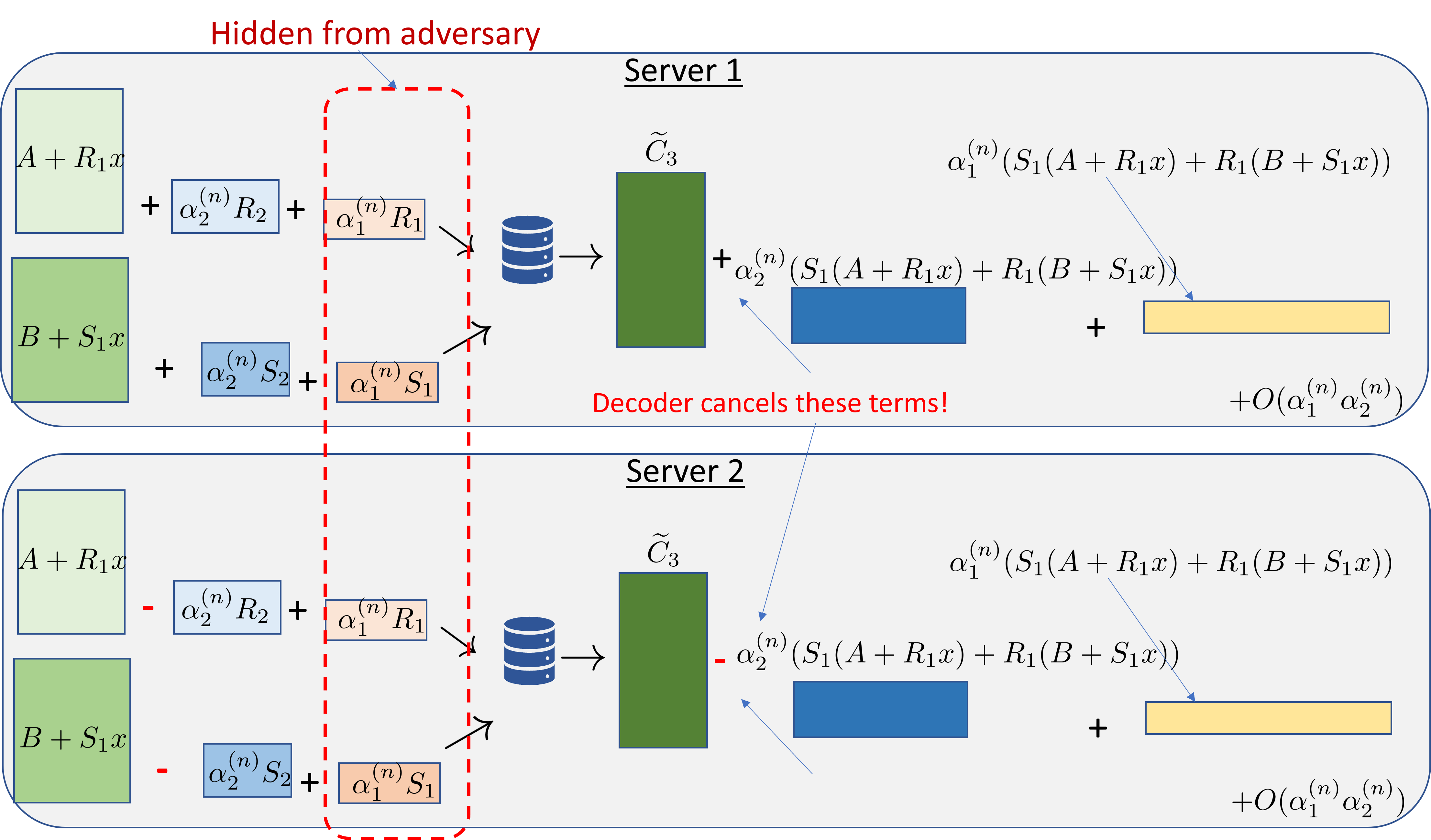
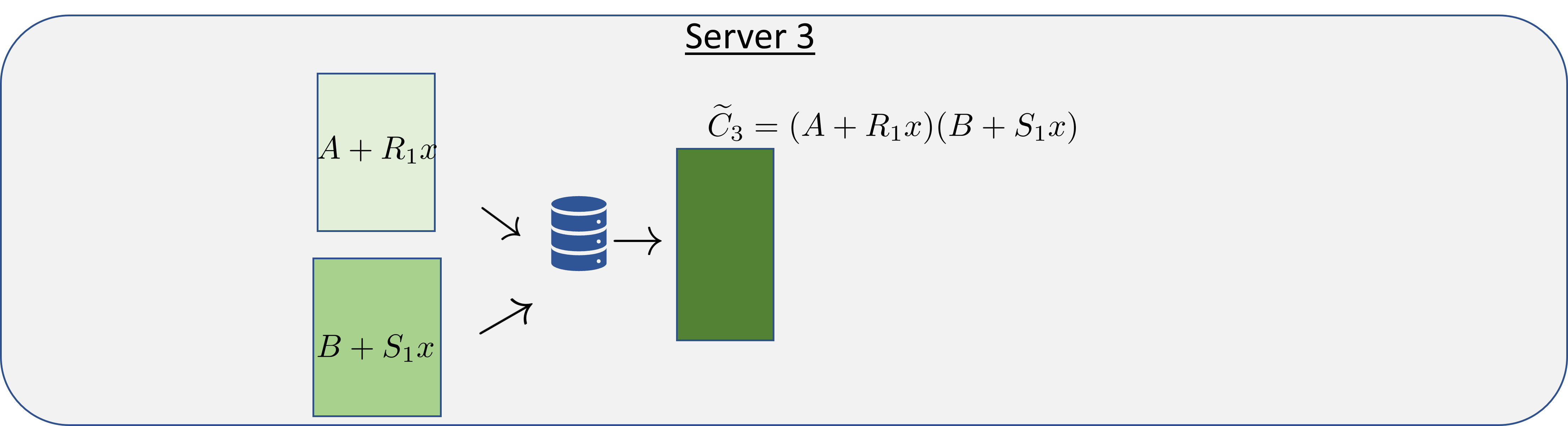
Figure 2: Pictorial depiction of the coding scheme for $t=2,N=3$ with matrix $\mathbf{G}=\begin{bmatrix}1&-1\end{bmatrix}$.

3.2 Privacy Analysis

Informal privacy analysis: For expository purposes, we first provide a coarse privacy analysis with informal reasoning. With the above scheme, we claim that $\texttt{SNR}_{p}\approx\eta/x^{2},$ and so, it suffices to choose $x\approx\sqrt{\frac{\eta}{\texttt{SNR}_{p}}}.$ Consider $A$’s privacy constraint, we require $\texttt{SNR}_{\mathcal{S}}^{A}\leq\texttt{SNR}_{p}$ for every $\mathcal{S}\subset\{1,2,\ldots,N\},|\mathcal{S}|=t$. First we consider the scenario where $\mathcal{S}=\{1,2,\ldots,t\}$. Each node’s input is of the form $A+R_{1}(x+\alpha_{1}^{(n)})+\alpha_{2}^{(n)}\begin{bmatrix}R_{2}&R_{3}&\ldots&R_{t}\end{bmatrix}\vec{g}_{i}.$ Even if an adversary with access to the inputs to nodes in $\mathcal{S}$ happens to know $R_{2},R_{3},\ldots,R_{t}$, but not $R_{1},$ the noise $(x+\alpha_{1}^{(n)})R_{1}$ provides enough privacy, that is the privacy signal to noise ratio for this set is $\approx\eta/x^{2}$ for sufficiently large $n$.

Now, consider the cases where the set $\mathcal{S}$ of $t$ colluding adversaries includes node $t+1$. In this case, the adversary has $A+R_{1}x$ from node $t+1.$ The other $t-1$ colluding nodes have inputs: $A+R_{1}(x+\alpha_{1}^{(n)})+\alpha_{2}^{(n)}\begin{bmatrix}R_{2}&R_{3}&\ldots R_{3}&\ldots&R_{t}\end{bmatrix}\vec{g}_{i}$ for $i\in\mathcal{S}-\{t+1\}.$ Informally, this can be written as $A+R_{1}x+R_{1}\alpha_{1}^{(n)}+\Omega(\alpha_{2}^{(n)})Z_{i},$ for some random variable $Z_{i}$ with variance $\Theta(1)$.

On the one hand, observe that these $t-1$ nodes contain a linear combination of $A,R_{1}$ that is linearly independent of the input to the $(t+1)$-th node (which is $A+xR_{1}$). It might seem possible for the adversary to increase its signal-to-noise ratio beyond $\frac{\eta}{x^{2}}$ by combining the input of these $t-1$ nodes with node $t+1$’s input. However, observe crucially that the first layer of the inputs to these $t-1$ nodes is linearly dependent with $t+1$’s input. The privacy signal-to-noise ratio can be increased by a non-negligible extent at the adversary only if it is able to access information in the third layer. Since $|\alpha_{2}^{(n)}|\gg|\alpha_{1}^{(n)}|$, in order to access the information in the third layer and reduce/cancel the effect of $R_{1}$, the adversary must first be able to cancel the second layer terms whose magnitude is $\Omega(\alpha_{2}^{(n)})$. But these second layer terms are a combination of $t-1$ independent noise variables $R_{2},R_{3},\ldots,R_{t}$ that are modulated by linearly independent vectors. Hence, any non-trivial linear combination of these $t-1$ inputs necessarily contains a non-zero $\Omega(\alpha_{2}^{(n)})$ additive noise term. So, their effect cannot be canceled and the $\alpha_{1}^{(n)}R_{1}$ term in the third layer is hidden from the decoder (See Fig. 2). Consequently, as $n\to\infty$, the input to these $t-1$ nodes is, approximately, a statistically degraded version of $A+xR_{1}$. Therefore, the parameter $\texttt{SNR}_{p}$ cannot be increased beyond $\frac{\eta}{x^{2}}.$

Formal privacy analysis: We now present a formal privacy analysis. We show that for any $\delta>0$, by taking $n$ sufficiently large, we can ensure that:

$$\texttt{SNR}_{\mathcal{S}}^{(A)},\texttt{SNR}_{\mathcal{S}}^{(B)}\leq\frac{\eta}{x^{2}}+\delta$$

for every subset $\mathcal{S}$ of $t$ nodes. Because of the symmetry of the coding scheme, it suffices to show that $\texttt{SNR}_{\mathcal{S}}^{(A)}$ satisfies the above relation. In our analysis, we will repeatedly use the fact that any linear combination $\sum_{i\in\mathcal{S}}\beta_{i}\tilde{A}_{i}$ of the inputs to the adversary satisfies:

$$\mathbb{E}\left[\left(\left(\sum_{i\in\mathcal{S}}\beta_{i}\tilde{A}_{i}\right)-A\right)^{2}\right]\geq\frac{\eta}{1+\texttt{SNR}_{\mathcal{S}}^{(A)}}$$

First consider the case where $t+1\notin\mathcal{S}$. For each $i\in\mathcal{S},$ the input $\tilde{A}_{i}$ is of the form $A+(x+\alpha_{1}^{(n)})R_{1}+Z_{i},$ where $Z_{i}$ is zero mean random variable that is statistically independent of $R_{1}.$ Therefore, we have:

$$\inf_{\beta_{i}\in\mathbb{R},i\in\mathcal{S}}\mathbb{E}\left[\left(\left(\sum_{j\in\mathcal{S}}\beta_{j}\tilde{A}_{j}\right)-A\right)^{2}\right]$$

$$\geq\inf_{\beta\in\mathbb{R}}\mathbb{E}\left[\left(\beta(A+(x+\alpha_{i}^{(n)})R_{1})-A\right)^{2}\right]$$

$$=\frac{\eta}{1+\frac{\eta}{(x+\alpha_{i}^{(n)})^{2}}}\geq\frac{\eta}{1+\frac{\eta}{x^{2}}}.$$

Consequently: $\texttt{SNR}_{\mathcal{S}}^{(A)}\leq\frac{\eta}{x^{2}}.$

Now consider the case: $t+1\in\mathcal{S}$. Consider a linear estimator:

$$\hat{A}= \beta_{t+1}(A+xR_{1})+\sum_{i\in\mathcal{S}\setminus\{t+1\}}\beta_{i}\left(A+R_{1}(x+\alpha_{1}^{(n)})+\alpha_{2}^{(n)}\begin{bmatrix}R_{2}&R_{3}&\ldots&R_{t}\end{bmatrix}\vec{g}_{i}\right)$$

$$= A\left(\sum_{i\in\mathcal{S}}\beta_{i}\right)+R_{1}\left(x\sum_{i\in\mathcal{S}}\beta_{i}+\alpha_{1}^{(n)}\sum_{i\in\mathcal{S}\setminus\{t+1\}}\beta_{i}\right)+\alpha_{2}^{(n)}\begin{bmatrix}R_{2}&R_{3}&\ldots&R_{t}\end{bmatrix}\left(\sum_{i\in\mathcal{S}\setminus\{t+1\}}\beta_{i}\vec{g}_{i}\right)$$

Because of property (C1), there are only two possibilities: (i) $\beta_{i}=0,$ for all $i\in\mathcal{S}\setminus\{t+1\}$, or (ii) $\left(\sum_{i\in\mathcal{S}\setminus\{t+1\}}\beta_{i}\vec{g}_{i}\right)\neq 0$. In the former case, the linear combination is $\hat{A}=\beta_{t+1}(A_{t+1}+xR_{1})$ from which, the best linear estimator has signal to noise ratio $\eta/x^{2}$ as desired. Consider the latter case, let $\rho>0$ be the smallest singular value among the singular values of all the $(t-1)\times(t-1)$ sub-matrices of $\mathbf{G}$. We bound the noise power of $\hat{A}$ below; in these calculations, we use the fact that $R_{i}$ are zero-mean unit variance uncorrelated random variables for $i=1,2,\ldots,t$.

$$\left(x\sum_{i\in\mathcal{S}}\beta_{i}+\alpha_{1}^{(n)}\sum_{i\in\mathcal{S}\setminus\{t+1\}}\beta_{i}\right)^{2}+(\alpha_{2}^{(n)})^{2}\mathbb{E}\left[\left(\begin{bmatrix}R_{2}&R_{3}&\ldots&R_{t}\end{bmatrix}\sum_{i\in\mathcal{S}\setminus\{t+1\}}\beta_{i}\vec{g}_{i}\right)^{2}\right]$$

$$=\left(x\sum_{i\in\mathcal{S}}\beta_{i}+\alpha_{1}^{(n)}\sum_{i\in\mathcal{S}\setminus\{t+1\}}\beta_{i}\right)^{2}+(\alpha_{2}^{(n)})^{2}\left|\left|\sum_{i\in\mathcal{S}\setminus\{t+1\}}\beta_{i}\vec{g}_{i}\right|\right|^{2}$$

$$\geq\left(x\sum_{i\in\mathcal{S}}\beta_{i}+\alpha_{1}^{(n)}\sum_{i\in\mathcal{S}\setminus\{t+1\}}\beta_{i}\right)^{2}+(\alpha_{2}^{(n)})^{2}\rho^{2}\sum_{i\in\mathcal{S}\setminus\{t+1\}}\beta_{i}^{2}$$

The signal-to-noise ratio for signal $A$ in $\hat{A}$ can be bounded as:

$$\frac{\eta\left(\sum_{i\in\mathcal{S}}\beta_{i}\right)^{2}}{\left(x\sum_{i\in\mathcal{S}}\beta_{i}+\alpha_{1}^{(n)}\sum_{i\in\mathcal{S}\setminus\{t+1\}}\beta_{i}\right)^{2}+(\alpha_{2}^{(n)})^{2}\rho^{2}\sum_{i\in\mathcal{S}\setminus\{t+1\}}\beta_{i}^{2}}$$

$$\stackrel{{\scriptstyle(a)}}{{\leq}} \frac{\eta\left(\sum_{i\in\mathcal{S}}\beta_{i}\right)^{2}}{x^{2}\left(\sum_{i\in\mathcal{S}}\beta_{i}\right)^{2}+2x\alpha_{1}^{(n)}\left(\sum_{i\in\mathcal{S}\setminus\{t+1\}}\beta_{i}\right)\left(\sum_{i\in\mathcal{S}}\beta_{i}\right)+(\alpha_{2}^{(n)})^{2}\rho^{2}\sum_{i\in\mathcal{S}\setminus\{t+1\}}\beta_{i}^{2}}$$

$$= \frac{\eta}{x^{2}+2x\alpha_{1}^{(n)}\nu_{1}+(\alpha_{2}^{(n)})^{2}\rho^{2}\nu_{2}^{2}}\stackrel{{\scriptstyle(b)}}{{\leq}}\frac{\eta}{x^{2}-2x\alpha_{1}^{(n)}\sqrt{t}\nu_{2}+(\alpha_{2}^{(n)})^{2}\rho^{2}\nu_{2}^{2}}\stackrel{{\scriptstyle(c)}}{{\leq}}\frac{\eta}{x^{2}-\frac{(\alpha_{1}^{(n)})^{2}}{(\alpha_{2}^{(n)})^{2}}\frac{x^{2}t}{\rho^{2}}}$$

The upper bound of (a) holds because we have replaced the denominator by a smaller quantity. In (b), we have used the fact that $\nu_{1}^{2}\leq t\nu_{2}^{2}$ and consequently $-\sqrt{t}\nu_{2}\leq\nu_{1}\leq\sqrt{t}\nu_{2}.$ (c) holds because

$$\inf_{\nu_{2}}(\alpha_{2}^{(n)})^{2}\rho^{2}\nu_{2}^{2}-2x\alpha_{1}^{(n)}\sqrt{t}\nu_{2}=-\frac{x^{2}(\alpha_{1}^{(n)})^{2}t}{(\alpha_{2}^{(n)})^{2}\rho^{2}}.$$

As $n\to\infty,$ (3.12) implies that $\frac{(\alpha_{1}^{(n)})^{2}}{(\alpha_{2}^{(n)})^{2}}\to 0$, and consequently, for any $\delta>0,$ we can choose a sufficiently large $n$ to ensure that the right hand side of $(c)$ can be made smaller than $\frac{\eta}{x^{2}}+\delta$. Thus, for sufficiently large $n$, $\texttt{SNR}_{p}\leq\frac{\eta}{x^{2}}+\delta$ for any $\delta>0.$

3.3 Accuracy Analysis

To show the theorem, it suffices to show that for any $\delta>0,$ we can obtain $\texttt{SNR}_{a}\geq\frac{(x^{2}+\eta)^{2}}{x^{4}}-1-\delta$

Informal Accuracy Analysis We provide a high-level description of the accuracy analysis for the case of $t=2,N=3.$ We assume that $\mathbf{G}=[1~{}~{}-1]$ like in Fig. 2. The computation outputs of the three nodes are:

$$\widetilde{C}_{1} =(A+R_{1}(x+\alpha_{1}^{(n)})+\alpha_{2}^{(n)}R_{2})(B+S_{1}(x+\alpha_{1}^{(n)})+\alpha_{2}^{(n)}R_{2})$$

$$=\underbrace{\widetilde{C}_{3}}_{\text{First layer}}+\underbrace{\alpha_{2}^{(n)}(S_{2}(A+R_{1}x)+R_{2}(B+S_{1}x))}_{\text{Second Layer}}+\underbrace{\alpha_{1}^{(n)}(S_{1}(A+R_{1}x)+R_{1}(B+S_{1}x))}_{\text{Third Layer}}+\underbrace{O(\alpha_{1}^{(n)}\alpha_{2}^{(n)})}_{\text{Fourth Layer}}$$

$$\widetilde{C}_{2} =(A+R_{1}(x+\alpha_{1}^{(n)})-\alpha_{2}^{(n)}R_{2})(B+S_{1}(x+\alpha_{1}^{(n)})-\alpha_{2}^{(n)}S_{2})$$

$$=\underbrace{\widetilde{C}_{3}}_{\text{First layer}}-\underbrace{\alpha_{2}^{(n)}(S_{2}(A+R_{1}x)+R_{2}(B+S_{1}x))}_{\text{Second Layer}}+\underbrace{\alpha_{1}^{(n)}(S_{1}(A+R_{1}x)+R_{1}(B+S_{1}x))}_{\text{Third Layer}}+\underbrace{O(\alpha_{1}^{(n)}\alpha_{2}^{(n)})}_{\text{Fourth Layer}}$$

$$\widetilde{C}_{3} =(A+R_{1}x)(B+S_{1}x)$$

In effect, at nodes $1$ and $2,$ the computation output can be interpreted as a superposition of at least $4$ layers. The first layer has magnitude $\Theta(1),$ the second $\Theta(\alpha_{2}^{(n)}),$ the third $\Theta(\alpha_{1}^{(n)}),$ and the remaining layers have magnitude $O(\alpha_{1}^{(n)}\alpha_{2}^{(n)}).$ The decoder can eliminate the effect of the second layer by computing:

$$\overline{C}=\frac{\widetilde{C}_{1}+\widetilde{C}_{2}}{2}=(A+R_{1}(x+\alpha_{1}^{(n)}))(B+S_{1}(x+\alpha_{1}^{(n)}))+o(\alpha_{1}^{(n)})$$

Notice that the decoder also has access to $\tilde{C}_{3}=(A+R_{1}x)(B+S_{1}x)$. From $\overline{C}$ and $\tilde{C}_{3},$ the decoder can approximately compute:

$$\overline{\overline{C}}\approx\frac{d}{dx}\left((A+R_{1}x)(B+S_{1}x)\right)=(AS_{1}+BR_{1})+2R_{1}S_{1}x$$

A simple calculation of the noise covariance matrix reveals that from $\overline{\overline{C}}$ and $C_{3}$, the decoder can compute $AB$ with $\texttt{SNR}_{a}\approx\frac{\eta^{2}}{x^{4}}+\frac{2\eta}{x^{2}}$ as desired.

Formal Accuracy Analysis

To show the theorem statement, it suffices to show that for any $\delta>0,$ we can achieve $\texttt{SNR}_{a}>2\frac{\eta}{x^{2}}+\frac{\eta^{2}}{x^{4}}-\delta$ for a sufficiently large $n$. We show this next by constructing a specific linear combination of the observations that achieves the desired signal-to-noise ratio. Observe that with our coding scheme, the nodes compute:

$$\Gamma_{t+1}\Theta_{t+1}=(A+R_{1}x)(B+S_{1}x)$$

and, for $i=1,\ldots,t$:

$$\Gamma_{i}\Theta_{i} =(A+R_{1}(x+\alpha_{1}^{(n)}))(B+S_{1}(x+\alpha_{1}^{(n)}))+\alpha_{2}^{(n)}\bigg{(}(A+R_{1}(x+\alpha_{1}^{(n)}))\begin{bmatrix}S_{2}&\ldots&S_{t}\end{bmatrix}$$

$$+(B+S_{1}(x+\alpha_{1}^{(n)}))\begin{bmatrix}R_{2}&\ldots&R_{t}\end{bmatrix}\bigg{)}\vec{g}_{i}+O((\alpha_{2}^{(n)})^{2})$$

Let $\gamma_{1},\gamma_{2},\ldots,\gamma_{t}$ be scalars, not all equal to zero, such that $\sum_{i=1}^{t}\gamma_{i}\vec{g}_{i}=0.$ Because $\vec{g}_{i}$ are $t-1$ dimensional vectors, they are linearly dependent, and such scalars indeed do exist. Condition (C2) implies that $\sum_{i=1}^{t}\gamma_{i}\neq 0.$ Without appropriate rescaling if necessary, we assume $\sum_{i=1}^{t}\gamma_{i}=1.$ The decoder computes: $\tilde{\Gamma}\tilde{\Theta}\stackrel{{\scriptstyle\Delta}}{{=}}\sum_{i=1}^{t}\gamma_{i}\Gamma_{i}\Theta_{i},$ which is equal to:

$$\tilde{\Gamma}\tilde{\Theta}=(A+R_{1}(x+\alpha_{1}^{(n)}))(B+S_{1}(x+\alpha_{1}^{(n)}))+O((\alpha_{2}^{(n)})^{2}).$$

Then, the signal-to-noise ratio achieved is at least that obtained by using the signal and noise covariance matrices of

$$\Gamma_{t+1}\Theta_{t+1} = AB+x(AS_{1}+BR_{1})+R_{1}S_{1}x^{2}$$ (3.17)

$$\tilde{\Gamma}\tilde{\Theta} = AB+(x+\alpha_{1}^{(n)})(AS_{1}+BR_{1})+(x+\alpha_{1}^{(n)})^{2}R_{1}S_{1}+O((\alpha_{2}^{(n)})^{2}).$$ (3.18)

The analysis is done in equations (3.19)-(3.20) next:

$$\texttt{SNR}_{a} \geq\frac{\begin{vmatrix}\eta^{2}+2\eta x^{2}+x^{4}&\eta^{2}+2\eta x(x+\alpha_{1}^{(n)})+x^{2}(x+\alpha_{1}^{(n)})^{2}\\ \eta^{2}+2\eta x(x+\alpha_{1}^{(n)})+x^{2}(x+\alpha_{1}^{(n)})^{2}&\eta^{2}+2\eta(x+\alpha_{1}^{(n)})^{2}+(x+\alpha_{1}^{(n)})^{4}+O((\alpha_{2}^{(n)})^{4})\end{vmatrix}}{\begin{vmatrix}2\eta x^{2}+x^{4}&2\eta x(x+\alpha_{1}^{(n)})+x^{2}(x+\alpha_{1}^{(n)})^{2}\\ 2\eta x(x+\alpha_{1}^{(n)})+x^{2}(x+\alpha_{1}^{(n)})^{2}&2\eta(x+\alpha_{1}^{(n)})^{2}+(x+\alpha_{1}^{(n)})^{4}+O((\alpha_{2}^{(n)})^{4})\end{vmatrix}}-1$$ (3.19)

$$=\frac{4\alpha_{1}^{(n)}x(\eta+2x^{2})+2(\eta+x^{2})^{2}+(\alpha_{1}^{(n)})^{2}(\eta+2x^{2})+O((\alpha_{2}^{(n)})^{4})}{2x^{2}(\alpha_{1}^{(n)}+x^{2})+O((\alpha_{2}^{(n)})^{4})}-1$$ (3.20)

As $n\to\infty$, observe that $\alpha_{1}^{(n)},\frac{(\alpha_{2}^{(n)})^{2}}{\alpha_{1}^{(n)}}\rightarrow 0.$ Using this in (3.20), for any $\delta>0$, there exists a sufficiently large $n$ to ensure that $\texttt{SNR}_{a}\geq\frac{2(x^{2}+\eta)^{2}}{2x^{4}}-1-\delta=\frac{\eta^{2}}{x^{4}}+\frac{2\eta}{x^{2}}-\delta.$ This completes the proof.

3.4 Proof of Corollary 2.2.1

Our proof involves a specific realization of random variables $R_{1},R_{2},\ldots,R_{t},S_{1},S_{2},\ldots,S_{t}$ that satisfies the conditions of the achievable scheme in Section 3.1. We couple this with a refined differential privacy analysis. The accuracy analysis remains the same as in the proof of Section 3.3. Here, in our description, we focus on describing $R_{1},R_{2},\ldots,R_{t}$ and showing that the $t$-node DP privacy constraints are satisfied for input $A$. A symmetric argument applies for input $B$ also.

For a fixed DP parameter $\epsilon$, let $x={\sigma^{*}(\epsilon)}+\delta^{\prime},$ for $\delta^{\prime}>0$. Section 3.2 shows that the scheme achieves accuracy $\texttt{SNR}_{a}\approx(1+\frac{\eta}{x^{2}})^{2}$, or more precisely:

$$\texttt{LMSE}(\mathcal{C})\leq\frac{\eta^{2}(\sigma^{*}(\epsilon))^{4}}{(\eta+(\sigma^{*}(\epsilon))^{2})^{2}}+\delta$$

by choosing $\delta^{\prime}$ sufficiently small. Now, it remains to show that a specific realization of $R_{1},R_{2},\ldots,R_{t}$ achieves $\epsilon$-DP. For a fixed value of parameter $x$, let $\epsilon^{*}$ be:

$$\epsilon^{*}=\inf_{Z,E[Z^{2}]\geq 1}\sup_{\mathcal{A},A_{0},A_{1}\in\mathbb{R},|{A}_{0}-A_{1}|\leq 1}\ln\left(\frac{\mathbb{P}(A_{0}+xZ)\in\mathcal{A}}{\mathbb{P}(A_{1}+xZ)\in\mathcal{A}}\right)$$

where the infimum is over all real-valued random variables $Z$ satisfying the variance constraint, and $\ln$ denotes the natural logarithm. Notice here that the noise variance $E[(x^{2}Z^{2})]=x^{2}$ is strictly larger than $(\sigma^{*}(\epsilon))^{2}$. Because $\sigma^{*}$ is a strictly monotonically decreasing function (see (2.11)), we have: $\epsilon^{*}<\epsilon$. Let $Z^{*}$ be the random variable that is the argument of the above minimization. We now consider the achievable scheme of Section 3.1 with $R_{1}$ taking the same distribution as $Z^{*}.$ We let $R_{2},R_{3},\ldots,R_{t}$ to be independent unit variance Laplace random variables that are independent of $R_{1}$. Note that by construction,

$$\sup_{\mathcal{A}\in\mathbb{R},-1\leq\lambda\leq 1}\frac{\mathbb{P}\left(A+xR_{1}\in\mathcal{A}\right)}{\mathbb{P}\left(A+xR_{1}+\lambda\in\mathcal{A}\right)}\leq e^{\epsilon^{*}}$$ (3.21)

Here, we are considering an adversary that is aiming to learn $A$ from $\tilde{A}_{i},i\in\mathcal{S}$ which for every $t$-sized subset $\mathcal{S}$. Let $\overline{\epsilon}_{n}$ be the parameter such that the coding scheme specified achieves $t$-node $\overline{\epsilon}_{n}$-DP. We show that as $n\to\infty$, $\overline{\epsilon}_{n}\to\epsilon^{*},$ thus showing that for sufficiently large $n$, our scheme achieves $t$-node $\epsilon$-DP .

First, consider the case where $t+1\notin\mathcal{S}$. For each $i\in\mathcal{S},$ the input $\tilde{A}_{i}$ is of the form $A+R_{1}(x+\alpha_{1}^{(n)})R_{1}+Z_{i},$ where $Z_{i}$ is zero mean random variable that is statistically independent of $R_{1}.$ Therefore,

$$A\rightarrow A+(x+\alpha_{1}^{(n)})R_{1}\rightarrow\{\tilde{A}_{i}:{i\in\mathcal{S}}\}$$

forms a Markov chain. Using post-processing property and the notation of (2.6),(2.7), we note that

$$\sup_{\mathcal{A}\in\mathbb{R}^{t}}\frac{\mathbb{P}\left(\mathbf{Y}^{(0)}_{\mathcal{S}}\in\mathcal{A}\right)}{\mathbb{P}\left(\mathbf{Y}^{(1)}_{\mathcal{S}}\in\mathcal{A}\right)}$$

$$\leq \sup_{\mathcal{A}\in\mathbb{R},-1\leq\lambda\leq 1}\frac{\mathbb{P}\left(A+(x+\alpha_{1}^{(n)})R_{1}\in\mathcal{A}\right)}{\mathbb{P}\left(A+(x+\alpha_{1}^{(n)})R_{1}+\lambda\in\mathcal{A}\right)}$$

$$= \sup_{\mathcal{A}\in\mathbb{R},-\frac{x}{x+\alpha_{1}^{(n)}}\leq\lambda\leq\frac{x}{x+\alpha_{1}^{(n)}}}\frac{\mathbb{P}\left(A+xR_{1}\in\mathcal{A}\right)}{\mathbb{P}\left(A+xR_{1}+\lambda\in\mathcal{A}\right)}$$

$$\leq e^{\epsilon^{*}}$$

where, in the final inequality, we have used (3.21) combined with the fact that: $0<\frac{x}{x+\alpha_{1}^{(n)}}\leq 1$ Thus, the input to the adversary follows $t$ node $\epsilon^{*}$-DP.

Now, consider the case where $t+1\in\mathcal{S}$. To keep the notation simple, without loss of generality, we assume that $\mathcal{S}=\{2,3,\ldots,t+1\}.$ We denote

$$\mathbf{G}_{2:t}=\begin{bmatrix}\vec{g}_{2}&\vec{g}_{3}&\ldots&\vec{g}_{t}\end{bmatrix}$$

In this case, an adversary obtains

$$\vec{Z} = \left(A+R_{1}x,A+(x+\alpha_{1}^{(n)})R_{1}\right.\left.~{}+\alpha_{2}^{(n)}\begin{bmatrix}R_{2}&R_{3}&\ldots&R_{t}\end{bmatrix}\mathbf{G}_{2:t}\right).$$

Using the fact that $\mathbf{G}_{2:t}$ is invertible based on the property (C1) in Section 3.1, a one-to-one function on the adversary’s input yields:

$$\vec{Z^{\prime}}=\left(A+R_{1}x,-\frac{\alpha_{1}^{(n)}}{\alpha_{2}^{(n)}x}A\vec{1}(\mathbf{G}_{2:t})^{-1}+\begin{bmatrix}R_{2}&R_{3}&\ldots&R_{t}\end{bmatrix}\right),$$

where $\vec{1}$ is a $t-1\times 1$ row vector. Denoting $\vec{Z^{\prime}}=(Z^{\prime}_{1},Z^{\prime}_{2},\ldots,Z^{\prime}_{t})$, observe that $Z_{i}^{\prime}=\lambda_{i}A+\zeta_{i}R_{i}$ for some $\lambda_{i},\zeta_{i}\in\mathbb{R}$. By construction $Z^{\prime}_{1}$ achieves $\epsilon^{*}$-DP. For $i\geq 2$, because $R_{i}$ is a unit variance Laplacian RV, $Z_{i}^{\prime}$ is a privacy mechanism that achieves $\frac{\alpha_{i}}{\beta_{i}}\sqrt{2}$-DP with respect to input $A$. Because $R_{1},R_{2},\ldots,R_{t}$ are independent, $\vec{Z^{\prime}}$ is an RV that achieves $\epsilon^{*}+\sqrt{2}\sum_{i=2}^{t}\frac{\alpha_{i}}{\beta_{i}}$-DP. Note that for $i\geq 2,$ $\lambda_{i}^{\prime}=1$ and $\zeta_{i}=\frac{\alpha_{1}^{(n)}g_{i}^{\prime}}{\alpha_{2}^{(n)}x},$ where, $g_{i}^{\prime}$ is the $i$-th element of $\vec{1}(\mathbf{G}_{2:t})^{-1})$. So, the adversary’s input satisfies $t$-node $\epsilon^{*}+\sqrt{2}\sum_{i=2}^{t}\frac{\alpha_{1}^{(n)}g_{i}^{\prime}}{\alpha_{2}^{(n)}x}$-DP. The proof is complete on noting that the DP parameter approaches $\epsilon^{*}$ as $n\to\infty$.

4 Proofs of Theorem 2.3 and Corollary 2.3.1

Recall that we consider a set up with $N$ computation nodes such that the input is private to any $t$ nodes, where $N\leq 2t.$ Consider an achievable scheme that achieves $t$-node privacy signal-to-noise ratio $0<\texttt{SNR}_{p}<\infty$ and accuracy signal-to-noise ratio $\texttt{SNR}_{a}.$ There exist uncorrelated, zero-mean, unit-variance random variables $\overline{R}_{1},\overline{R}_{2},\ldots,\overline{R}_{N},\overline{S}_{1},\overline{S}_{2},\ldots,\overline{S}_{N}$ such that $A,B,\overline{R}_{i}\big{|}_{i=1}^{t},S_{i}\big{|}_{i=1}^{t}$ are zero mean unit variance uncorrelated random variables, and the inputs to node $i$ are:

$$\Gamma_{i}=\left[\frac{A}{\sqrt{\eta}}~{}\overline{R}_{1}~{}\overline{R}_{2}~{}\ldots~{}\overline{R}_{N}\right]\vec{v}_{i}$$

$$\Theta_{i}=\left[\frac{B}{\sqrt{\eta}}~{}\overline{S}_{1}~{}\overline{S}_{2}~{}\ldots~{}\overline{S}_{N}\right]\vec{w}_{i}$$

where $\vec{v}_{i},\vec{w}_{i}$ are $N\times 1$ vectors. Node $i$ performs the computation

$$\tilde{C}_{i}=\Gamma_{i}\Theta_{i},$$

and a decoder connects to the $N$ nodes and obtains:

$$\widetilde{C}=\sum_{i=1}^{N}d_{i}\Lambda_{i}$$

The error $\widetilde{C}-AB$ of the decoder can be written as:

$$\widetilde{C}-AB=\left[\frac{A}{\sqrt{\eta}}~{}\overline{R}_{1}~{}\overline{R}_{2}~{}\ldots~{}\overline{R}_{N}\right]\Delta\begin{bmatrix}\frac{B}{\sqrt{\eta}}\\ \overline{S}_{1}\\ \overline{S}_{2}\\ \vdots\\ \overline{S}_{N}\end{bmatrix}$$

where

$$\Delta=\sum_{i=1}^{N}d_{i}\vec{v}_{i}\vec{w}_{i}^{T}-\begin{bmatrix}\eta&0&\ldots&0\\ 0&0&\ldots&0\\ &&\ddots&\\ 0&0&\ldots&0\end{bmatrix}$$

Observe that, for the optimal choice of $d_{1},d_{2},\ldots,d_{N}$,

$$\mathbb{E}\left[||\widetilde{C}-AB||^{2}\right]=||\Delta||_{F}^{2}=\frac{\eta^{2}}{1+\texttt{SNR}_{a}}.$$

We aim to lower bound $||\Delta||_{F}^{2}.$ Our converse is a natural consequence of the following theorem.

Theorem 4.1.

For any $N$ node secure coding scheme with $N\leq 2t$, for any set $\mathcal{S}\subset\{1,2,\ldots,N\}$ where $|\mathcal{S}|=t,$ we have:

$$(1+\texttt{SNR}_{a})\leq(1+\texttt{SNR}^{(A)}_{\mathcal{S}})(1+\texttt{SNR}^{(B)}_{\mathcal{S}^{c}})$$

By symmetry, we also have:

$$(1+\texttt{SNR}_{a})\leq(1+\texttt{SNR}^{(B)}_{\mathcal{S}})(1+\texttt{SNR}^{(A)}_{\mathcal{S}^{c}})$$

For any coding scheme that that satisfies $\texttt{SNR}^{(A)}_{\mathcal{S}},\texttt{SNR}^{(B)}_{\mathcal{S}}\leq\texttt{SNR}_{p}$ for every subset $\mathcal{S}$ of $t$ nodes, the above theorem automatically implies the statement of Theorem 2.3, that is:

$$(1+\texttt{SNR}_{a})\leq(1+\texttt{SNR}_{p})^{2}$$

The proof of Theorem 4.1 depends on the following key lemma.

Lemma 4.2.

For any set $\mathcal{S}$ of nodes with $|\mathcal{S}|\leq t,$ there exists a vector

$$\vec{\lambda}=\left[\lambda_{1}~{}~{}\lambda_{2}~{}~{}\ldots~{}~{}\lambda_{N}\right]^{T}$$

such that

1. $$\vec{\lambda}^{T}\vec{w}_{i}=0,\forall i\in\mathcal{S},$$

2. $$\frac{\lambda_{1}^{2}}{||\vec{\lambda}||^{2}}\geq\frac{1}{1+\texttt{SNR}^{(B)}_{\mathcal{S}}}.$$

Symmetrically, there exists a vector

$$\vec{\theta}=\left[\theta_{1}~{}~{}\theta_{2}~{}~{}\ldots~{}~{}\theta_{t+1}\right]^{T}$$

for every subset $\mathcal{S}$ of nodes with $|\mathcal{S}|\leq t$ such that

1. $$\vec{\theta}^{T}\vec{v}_{i}=0,\forall i\in\mathcal{S},$$

2. $$\frac{\theta_{1}^{2}}{||\vec{\theta}||^{2}}\geq\frac{1}{1+\texttt{SNR}^{(A)}_{\mathcal{S}}}.$$

Proof.

For any vector $\vec{\underline{w}}=[\underline{w}_{1}~{}~{}\underline{w}_{2}~{}~{}\ldots~{}~{}\underline{w}_{N}]^{T}$ that in the span of $\{\vec{w}_{i}:i\in\mathcal{S}\}$, we have:

$$\frac{{\underline{w}}_{1}^{2}}{\underline{w}_{2}^{2}+\underline{w}_{3}^{2}+\ldots+\underline{w}_{N}^{2}}\leq\texttt{SNR}^{(B)}_{\mathcal{S}}$$ (4.22)

Because $|\mathcal{S}|\leq t,$ the nullspace of $\{\vec{w}_{i}:i\in\mathcal{S}\}$ is non-trivial. If $\begin{bmatrix}1\\ 0\\ 0\\ \vdots\\ 0\end{bmatrix}$ lies in the span of $\{\vec{w}_{i}:i\in\mathcal{S}\}$, then $\texttt{SNR}^{(B)}_{\mathcal{S}}=\infty,$ and any non-zero vector $\vec{\lambda}$ in the null space of $\{\vec{w}_{i}:i\in\mathcal{S}\}$ satisfies $(i)$ and $(ii)$. So, it suffices to show the existence of the $\vec{\lambda}$ that satisfies the theorem for the case where $\begin{bmatrix}1\\ 0\\ 0\\ \vdots\\ 0\end{bmatrix}$ does not lie in the span of $\{\vec{w}_{i}:i\in\mathcal{S}\}$.

By the rank-nullity theorem, there exists a vector $\vec{\underline{w}}=[\underline{w}_{1}~{}~{}\underline{w}_{2}~{}~{}\ldots~{}~{}\underline{w}_{N}]^{T}$ in the span of $\{\vec{w}_{i}:i\in\mathcal{S}\},$ and a non-zero vector $\vec{\lambda}=\left[\lambda_{1}~{}~{}\lambda_{2}~{}~{}\ldots~{}~{}\lambda_{N}\right]^{T}$ that is in the nullspace of $\{\vec{w}_{i}:i\in\mathcal{S}\},$ such that

$$\vec{\underline{w}}+\vec{\lambda}=\begin{bmatrix}1\\ 0\\ 0\\ \vdots\\ 0\end{bmatrix}$$ (4.23)

Specifically, note that $\lambda_{i}=-\underline{w}_{i},$ for $i=2,3,\ldots,t+1.$ Because $\vec{\lambda}$ nulls $\vec{\underline{w}}$, we have:

$$\lambda_{1}\underline{w}_{1}=-\sum_{i=2}^{N}\lambda_{i}\underline{w}_{i}$$

Consequently, we have:

$$\lambda_{1}\underline{w}_{1}=\sum_{i=2}^{N}\underline{w}_{i}^{2}=\sum_{i=2}^{N}\lambda_{i}^{2}$$ (4.24)

Therefore:

$$\frac{||\vec{\lambda}||^{2}}{\lambda_{1}^{2}} =1+\frac{\sum_{i=2}^{N}\lambda_{i}^{2}}{\lambda_{1}^{2}}$$ (4.25)

$$=1+\frac{\sum_{i=2}^{N}\underline{w}_{i}^{2}}{\lambda_{1}^{2}}$$ (4.26)

$$=1+\frac{\underline{w}_{1}^{2}}{\sum_{i=2}^{N}\underline{w}_{i}^{2}}$$ (4.27)

$$\leq 1+\texttt{SNR}^{(B)}_{\mathcal{S}}$$ (4.28)

where in (4.26) and (4.27), we have used (4.24).

Therefore:

$$\frac{\lambda_{1}^{2}}{||\vec{\lambda}||^{2}}\geq\frac{1}{1+\texttt{SNR}^{(B)}_{\mathcal{S}}}$$

as required. The existence of a vector

$$\vec{\theta}^{(A)}_{\mathcal{S}}=\left[\theta_{1}~{}~{}\theta_{2}~{}~{}\ldots~{}~{}\theta_{t+1}\right]$$

that satisfies (iii),(iv) in the lemma statement follows from symmetry. ∎

Proof of Theorem 4.1.

Consider a set $\mathcal{S}$ of $t$ nodes. Let

$$\vec{\lambda}=\left[\lambda_{1}~{}~{}\lambda_{2}~{}~{}\ldots~{}~{}\lambda_{N}\right]^{T}$$

be a $N\times 1$ vector that is orthogonal to $\vec{w}_{\mathcal{S}^{c}}$ such that:

$$\frac{\lambda_{1}^{2}}{||\vec{\lambda}||^{2}}\geq\frac{1}{1+\texttt{SNR}^{(B)}_{\mathcal{S}^{c}}}$$ (4.30)

Because $|\mathcal{S}|=t$ and $N\leq 2t,$ it transpires that $|\mathcal{S}^{c}|\leq t,$ and from Lemma 4.2, we know that a vector $\vec{\lambda}$ satisfying the above conditions exist. We then have:

$${\Delta}\vec{\lambda}=\sum_{i\in\mathcal{S}}c_{i}\vec{v}_{i}-\begin{bmatrix}\lambda_{1}\eta\\ 0\\ \vdots\\ 0\end{bmatrix}$$ (4.31)

where $c_{i}=d_{i}\vec{w}_{i}^{T}\vec{\lambda}$. Now, we know that:

$$\inf_{\overline{c}_{i}}\left|\left|\sum_{i\in\mathcal{S}}\overline{c}_{i}\vec{v}_{i}-\begin{bmatrix}\sqrt{\eta}\\ 0\\ 0\\ \vdots\\ 0\end{bmatrix}\right|\right|^{2}=\frac{\eta}{1+\texttt{SNR}^{(A)}_{\mathcal{S}}}$$

Consequently, we have:

$$\left|\left|\sum_{i\in\mathcal{S}}{c}_{i}\vec{v}_{i}-\begin{bmatrix}\lambda_{1}\eta\\ 0\\ 0\vdots\\ 0\end{bmatrix}\right|\right|^{2}\geq\frac{\lambda_{1}^{2}\eta^{2}}{1+\texttt{SNR}^{(A)}_{\mathcal{S}}}$$

Taking norms in (4.31) and applying the above, we get:

$$||{\Delta}\vec{\lambda}||^{2}\geq\frac{\lambda_{1}^{2}\eta^{2}}{1+\texttt{SNR}^{(A)}_{\mathcal{S}}}$$ (4.32)

By definition of the $\ell_{2}$ norm, we have

$$||{\Delta}\vec{\lambda}||^{2}\leq||\Delta||_{2}^{2}||\vec{\lambda}||^{2}$$

Because, for any matrix, its Frobenius norm is lower bounded by its $\ell_{2}$ norm, we have:

$$||{\Delta}||_{F}^{2}\geq\frac{\lambda_{1}^{2}}{||\vec{\lambda}||^{2}}\frac{\eta^{2}}{1+\texttt{SNR}^{(A)}_{\mathcal{S}}}$$ (4.33)

From (4.30), we have:

$$||{\Delta}||_{F}^{2}\geq\eta^{2}\frac{1}{1+\texttt{SNR}^{(B)}_{\mathcal{S}^{c}}}\frac{1}{1+\texttt{SNR}^{(A)}_{\mathcal{S}}}$$ (4.34)

∎

4.1 Proof of Corollary 2.3.1

Consider an achievable coding scheme $\mathcal{C}$ that achieves $t$-node $\epsilon$-DP. From Lemma 2.1, we know that:

$$\texttt{LMSE}(\mathcal{C})=\frac{\eta^{2}}{1+\texttt{SNR}_{a}}$$ (4.35)

From Theorem 2.3, we know that there exists a set $\mathcal{S}\subset\{1,2,\ldots,N\}$ such that (i) $\texttt{SNR}_{\mathcal{S}}^{(A)}\geq\sqrt{1+\texttt{SNR}_{a}}-1,$ or(ii) $\texttt{SNR}_{\mathcal{S}}^{(B.)}\geq\sqrt{1+\texttt{SNR}_{a}}-1$. Without loss of generality, assume that (i) holds for the coding scheme $\mathcal{C}.$ Consequently, there exist scalars $w_{i},i\in\mathcal{S}$ such that:

$$\sum_{i\in\mathcal{S}}w_{i}\tilde{A}_{i}=A+Z$$

where $Z$ is uncorrelated with $A$ and $\mathbb{E}[Z]^{2}\leq\frac{\eta}{\sqrt{1+\texttt{SNR}_{a}}-1}.$ By definition of the function $\sigma^{*}(\epsilon),$ we have:

$$(\sigma^{*}(\epsilon))^{2}\leq E[Z]^{2}\leq\frac{\eta}{\sqrt{1+\texttt{SNR}_{a}}-1}.$$ (4.36)

Combining (4.35) and (4.36), we get the desired result.

5 Extension to Matrix Multiplication

We consider the problem of computing the matrix product $\mathbf{A}\mathbf{B}$, where $\mathbf{A}\in\mathbb{R}^{M\times L}$ and show how our scalar case results extend to matrix multiplication application. Our main result is an equivalence between codes for scalar multiplication and matrix multiplication under certain assumptions on the matrix multiplication code. Notation: In the sequel, for a matrix $\mathbf{M}$, we denote the entry in its $i$-th row and $j$-th column by $\mathbf{M}[i,j].$

Let $\mathcal{C}$ be an arbitrary $N$-node secure multiplication coding scheme that achieves $t$-node $\epsilon$-DP and the accuracy $\texttt{SNR}_{a}$ for computing a scalar product $AB$. We define $\mathcal{C}_{\text{matrix}}$ as a matrix extension of $\mathcal{C}$ that applies the coding scheme $\mathcal{C}$ independently to each entry of the matrices $\mathbf{A}\in\mathbb{R}^{M\times L}$ and $\mathbf{B}\in\mathbb{R}^{L\times K}$. Specifically, node $i$ in $\mathcal{C}_{\text{matrix}}$ receives:

$$\tilde{\mathbf{A}}_{i}=a_{1}\mathbf{A}+\mathbf{R}_{i}$$

$$\tilde{\mathbf{B}}_{i}=a_{1}\mathbf{B}+\mathbf{S}_{i}$$

where the entries of $\mathbf{R}_{i}$ and the entries of $\mathbf{S}_{i}$ are chosen in an i.i.d. manner from the same distribution specified by $\mathcal{C},$ and the constants $a_{i},b_{i}$ are also specified in $\mathcal{C}$. We evaluate the performance of $\mathcal{C}_{\text{matrix}}$ using worst-case metrics for both privacy and accuracy as follows:

Definition 5.1.

(Matrix $t$-node $\epsilon$-DP) Let $\epsilon\geq 0$. A coding scheme with random noise variables

$$(\tilde{\mathbf{R}}_{1},\tilde{\mathbf{R}}_{2},\ldots,\tilde{\mathbf{R}}_{N}),(\tilde{\mathbf{S}}_{1},\tilde{\mathbf{S}}_{2},\ldots,\tilde{\mathbf{S}}_{N})$$

where $\tilde{\mathbf{R}}_{i}\in\mathbb{R}^{M\times L},\tilde{\mathbf{S}}_{i}\in\mathbb{R}^{L\times K}$ and scalars $a_{i},b_{i}\;(i\in\{1,\ldots,N\})$ satisfies matrix $t$-node $\epsilon$-DP if, for any $\mathbf{A}_{0},\mathbf{A}_{1}\in\mathbb{R}^{M\times L},\mathbf{B}_{0},\mathbf{B}_{1}\in\mathbb{R}^{L\times K}$ that satisfy $\left|\left|\begin{bmatrix}\mathbf{A}_{0}\\ \mathbf{B}_{0}^{T}\end{bmatrix}-\begin{bmatrix}\mathbf{A}_{1}\\ \mathbf{B}_{1}^{T}\end{bmatrix}\right|\right|_{\text{max}}\leq 1$,

$$\max\left(\max_{\begin{subarray}{c}m=1,\ldots,M\\ l=1,\ldots,L\end{subarray}}\left(\frac{\mathbb{P}\left(\mathbf{Y}^{(0)}_{\mathcal{T}}[m,l]\in\mathcal{A}\right)}{\mathbb{P}\left(\mathbf{Y}^{(1)}_{\mathcal{T}}[m,l]\in\mathcal{A}\right)}\right),\max_{\begin{subarray}{c}l=1,\ldots,L\\ k=1,\ldots,K\end{subarray}}\left(\frac{\mathbb{P}\left(\mathbf{Z}^{(0)}_{\mathcal{T}}[l,k]\in\mathcal{A}\right)}{\mathbb{P}\left(\mathbf{Z}^{(1)}_{\mathcal{T}}[l,k]\in\mathcal{A}\right)}\right)\right) \leq e^{\epsilon}$$ (5.37)

for all subsets $\mathcal{T}\subseteq\{1,2,\ldots,N\},|\mathcal{T}|=t$, for all subsets $\mathcal{A}\subset\mathbb{R}^{1\times t}$ in the Borel $\sigma$-field, where, for $\ell=0,1$,

$$\mathbf{Y}_{\mathcal{T}}^{(\ell)}[m,l] \triangleq \begin{bmatrix}a_{i_{1}}\mathbf{A}_{\ell}[m,l]+\mathbf{\tilde{R}}_{i_{1}}[m,l],&\ldots,&a_{i_{|\mathcal{T}|}}\mathbf{A}_{\ell}[m,l]+\mathbf{\tilde{R}}_{i_{|\mathcal{T}|}}[m,l]\end{bmatrix}$$ (5.38)

$$\mathbf{Z}_{\mathcal{T}}^{(\ell)}[l,k] \triangleq \begin{bmatrix}b_{i_{1}}\mathbf{B}_{\ell}[l,k]+\mathbf{\tilde{S}}_{i_{1}}[l,k],&\ldots,&b_{i_{|\mathcal{T}|}}\mathbf{B}_{\ell}[l,k]+\mathbf{\tilde{S}_{i_{|\mathcal{T}|}}}[l,k]\end{bmatrix},$$ (5.39)

where $\mathcal{T}=\{i_{1},i_{2},\ldots,i_{|\mathcal{T}|}\}.$

Definition 5.2 (Matrix LMSE.).

For a matrix coding scheme $\mathcal{C}_{\text{matrix}}$, we define the LMSE as follows:

$$\textsf{LMSE}(\mathcal{C}_{\text{matrix}})=\max_{\begin{subarray}{c}m=1,\ldots,M\\ k=1,\ldots,K\end{subarray}}\mathbb{E}[|(\mathbf{A}\mathbf{B})[m,k]-\tilde{\mathbf{C}}[m,k]|^{2}],$$ (5.40)

where $\tilde{\mathbf{C}}$ is a decoded matrix using an affine decoding scheme $d$.

Analogous to Assumption 2.1 in the scalar case, our accuracy analysis is contingent on the data $\mathbf{A},\mathbf{B}$ satisfying the following assumption.

Assumption 5.1.

$\mathbf{A}$ and $\mathbf{B}$ are statistically independent matrices of dimensions $M\times L$ and $L\times K$, and they satisfy:

1. $$\mathbb{E}\left[||\mathbf{A}||_{\text{max}}^{2}\right]\leq\eta,\;\mathbb{E}\left[||\mathbf{B}||_{\text{max}}^{2}\right]{\leq\eta},$$ (5.41)

   for a parameter $\eta>0$, and

2. $$\mathbb{E}[\mathbf{A}[m,i]\mathbf{A}[m,j]]\mathbb{E}[\mathbf{B}[i,k]\mathbf{B}[j,k]]=0,$$ (5.42)

   for all $1\leq i\neq j\leq L$ and $m=1,\cdots M,k=1,\cdots K$.

Assumption 5.1-(b) for instance holds if the entries of $\mathbf{A}$ are uncorrelated, or if the entries of $\mathbf{B}$ are uncorrelated. Our main result states that $\mathcal{C}_{\textrm{matrix}}$ attains an identical privacy and accuracy as $\mathcal{C}$

Theorem 5.1.

Consider any (scalar) multiplication coding scheme $\mathcal{C}$. Let $\mathcal{C}_{\textrm{matrix}}$ denote its matrix extension. Then,

1. $\mathcal{C}$ satisfies $t$-node $\epsilon$-DP if and only if $\mathcal{C}_{\textrm{matrix}}$ satisfies $t$-node matrix $\epsilon$-DP.

2. If $\mathbf{A},\mathbf{B}$ satisfy Assumption 5.1, then:

   $$\textrm{LMSE}(\mathcal{C}_{\textrm{matrix}})\leq\sup\textrm{LMSE}(\mathcal{C}),$$

   where the supremum on the right hand side is over all data distributions $\mathbb{P}_{A,B}$ that satisfy Assumption 2.1 with parameter $\eta.$ Further, the bound above is met with equality if every entry of $\mathbf{A},\mathbf{B}$ has standard deviation $\eta.$

The above theorem establishes an equivalence between the trade-off for matrix multiplication and the trade-off for scalar multiplication. Specifically, using Corollaries 2.2.1 and 2.3.1, we infer that for a fixed matrix DP parameter $\epsilon,$ the optimal LMSE for the matrix multiplication case is the same as for scalar multiplication, that is:

$$\textrm{LMSE}\approx\frac{\eta^{2}(\sigma^{*}(\epsilon))^{4}}{\eta+(\sigma^{*}(\epsilon))^{2}}^{2}.$$

The above equivalence must however be interpreted with some caveats. First, the equivalence assumes that the coding scheme for the matrix case extends the scalar strategy to each input matrix element in an independent manner. The question of whether correlation in the noise distribution can reduce the LMSE for a fixed DP parameter is left open. Second, the above trade-off requires Assumption (5.1)-(b). In some cases, this assumption may be justified - for example, if $\mathbf{B}$ has data samples drawn from some distribution in an i.i.d. manner. However, in some cases, this assumption of uncorrelated data may be too strong. The question of the optimal trade-off when this assumption is dropped remains open.

Proof of Theorem 5.1.

Proof of (i)

An elementary proof readily from the definition of matrix $t$-node $\epsilon$-DP and the matrix extension of the coding scheme $\mathcal{C}$. Specifically, let $(\overline{R}_{1},\overline{R}_{2},\ldots,\overline{R}_{N})$ and $(\overline{S}_{1},\overline{S}_{2},\ldots,\overline{S}_{N})$ denote the noise random variables of coding scheme $\mathcal{C}$. Let $(\mathbf{\tilde{R}}_{1},\ldots,\mathbf{\tilde{R}}_{N})$ and $(\mathbf{\tilde{S}}_{1},\ldots,\mathbf{\tilde{S}}_{N})$ denote the noise random variables of the coding scheme $\mathcal{C}_{\text{matrix}}.$

To show the “if” statement, assume that $\mathcal{C}$ satisfies $t$-node $\epsilon$-DP. We show that $\mathcal{C}_{\textrm{matrix}}$ also satisfies $t$-node $\epsilon$-DP. Let $\mathbf{A}_{0},\mathbf{A}_{1},\mathbf{B}_{0},\mathbf{B}_{1}$ denote matrices that satisfy $\left|\left|\begin{bmatrix}\mathbf{A}_{0}\\ \mathbf{B}_{0}^{T}\end{bmatrix}-\begin{bmatrix}\mathbf{A}_{1}\\ \mathbf{B}_{1}^{T}\end{bmatrix}\right|\right|_{\text{max}}\leq 1.$ For an arbitrary subset $\mathcal{A}$ of the Borel sigma field, let

$$m^{*},l^{*}=\text{argmax}_{\begin{subarray}{c}m=1,\ldots,M\\ l=1,\ldots,L\end{subarray}}\left(\frac{\mathbb{P}\left(\mathbf{Y}^{(0)}_{\mathcal{T}}[m,l]\in\mathcal{A}\right)}{\mathbb{P}\left(\mathbf{Y}^{(1)}_{\mathcal{T}}[m,l]\in\mathcal{A}\right)}\right),$$

$$l^{**},k^{**}=\text{argmax}_{\begin{subarray}{c}l=1,\ldots,L\\ k=1,\ldots,K\end{subarray}}\left(\frac{\mathbb{P}\left(\mathbf{Z}^{(0)}_{\mathcal{T}}[l,k]\in\mathcal{A}\right)}{\mathbb{P}\left(\mathbf{Z}^{(1)}_{\mathcal{T}}[l,k]\in\mathcal{A}\right)}\right).$$

For any set $\mathcal{T}=\{i_{1},i_{2},\ldots,i_{t}\}\subset\{1,2,\ldots,N\}$:

$$\max_{m=1,2,\ldots,M,l=1,2,\ldots,L}\frac{\mathbb{P}\left(\mathbf{Y}^{(0)}_{\mathcal{T}}[m^{*},l^{*}]\in\mathcal{A}\right)}{\mathbb{P}\left(\mathbf{Y}^{(1)}_{\mathcal{T}}[m^{*},l^{*}]\in\mathcal{A}\right)}$$

$$\stackrel{{\scriptstyle(a)}}{{=}}\frac{\mathbb{P}(\begin{bmatrix}a_{i_{1}}\mathbf{A}_{0}[m^{*},l^{*}]+\overline{R}_{i_{1}}&\ldots&a_{i_{t}}\mathbf{A}_{0}[m^{*},l^{*}]+\overline{R}_{i_{t}}\end{bmatrix}}{\mathbb{P}(\begin{bmatrix}a_{i_{1}}\mathbf{A}_{1}[m^{*},l^{*}]+\overline{R}_{i_{1}}&\ldots&a_{i_{t}}\mathbf{A}_{1}[m^{*},l^{*}]+\overline{R}_{i_{t}}\end{bmatrix})}$$

$$\stackrel{{\scriptstyle(b)}}{{\leq}}e^{\epsilon}.$$

In $(a)$ above, we have used the fact that $(\overline{R}_{i_{1}},\overline{R}_{i_{2}},\ldots,\overline{R}_{i_{t}})$ has the same distribution as
$(\mathbf{R}_{i_{1}}[m^{*},l^{*}],\mathbf{R}_{i_{2}}[m^{*},l^{*}],\ldots,\mathbf{R}_{i_{t}}[m^{*},l^{*}])$. In (b) we have used the fact that

$$|\mathbf{A}_{0}[m^{*},l^{*}]-\mathbf{A}_{1}[m^{*},l^{*}]|\leq\left|\left|\begin{bmatrix}\mathbf{A}_{0}\\ \mathbf{B}_{0}^{T}\end{bmatrix}-\begin{bmatrix}\mathbf{A}_{1}\\ \mathbf{B}_{1}^{T}\end{bmatrix}\right|\right|_{\text{max}}1,$$

coupled with the fact that $\mathcal{C}$ satisfies $t$-node $\epsilon$-DP.

A similar argument leads us to conclude that

$$\frac{\mathbb{P}\left(\mathbf{Z}^{(0)}_{\mathcal{T}}[l^{**},k^{**}]\in\mathcal{A}\right)}{\mathbb{P}\left(\mathbf{Z}^{(1)}_{\mathcal{T}}[l^{**},k^{**}]\in\mathcal{A}\right)})\leq e^{\epsilon},$$

from which we infer $\mathcal{C}_{\textrm{matrix}}$ it satisfies matrix $t$-node $\epsilon$-DP.

The “only if” statement also follows through a similar elementary argument, and the details are omitted here.

Proof of (ii) Our proof revolves around showing that the signal-to-noise ratio achieved in obtaining $\mathbf{C}[m,l]$ using coding scheme $\mathcal{C}_{\textrm{matrix}}$ is the same (for the worst case distribution $\mathbb{P}_{\mathbf{A},\mathbf{B}}$) as the SNR achieved by $\mathcal{C}$, where $\mathbf{C}=\mathbf{A}\mathbf{B}.$ Consider scalar random variables $A,B$ that satisfy Assumption 2.1 with $\mathbb{E}[A^{2}]=\mathbb{E}[B^{2}]=\eta.$ let $(\overline{R}_{1},\overline{R}_{2},\ldots,\overline{R}_{N})$ and $(\overline{S}_{1},\overline{S}_{2},\ldots,\overline{S}_{N})$ denote the noise random variables of coding scheme $\mathcal{C}$. Denote by $\overline{\mathbf{K_{1}}}$ and $\overline{\mathbf{K_{2}}}$ as the covariance matrices of the coding scheme $\mathcal{C}$ as given in (2.9). As per definition 2.4,

$$\texttt{SNR}_{a}=\frac{\text{det}(\overline{\mathbf{K}}_{1})}{\text{det}(\overline{\mathbf{K}}_{2})}-1.$$

For $1\leq n_{1},n_{2}\leq N$, the $(n_{1},n_{2})$-th entry in the matrix $\overline{\mathbf{K}}_{1}$ is in the form of

$$\mathbb{E}\left[\left((A+\overline{R}_{n_{1}})(B+\overline{S})\right)^{2}\right]\;\;\text{ if $n_{1}=n_{2}$ or }\;\;\mathbb{E}\left[\left((A+\overline{R}_{n_{1}})(B+\overline{S}_{n_{1}})\right)\left((A+\overline{R}_{n_{2}})(B+\overline{S}_{n_{2}})\right)\right]~{}\text{ if $n_{1}\neq n_{2}$},$$ (5.43)

and the entries in the $\overline{\mathbf{K}}_{2}$ have the form of

$$\mathbb{E}\left[\left((A+\overline{R}_{n_{1}})(B+\overline{S}_{n_{1}})-AB\right)^{2}\right]\;\;\text{if $n_{1}=n_{2}$ or } \mathbb{E}\left[\left((A+\overline{R}_{n_{1}})(B+\overline{S}_{n_{1}})-AB\right)\left((A+\overline{R}_{n_{2}})(B+\overline{S}_{n_{2}})-AB\right)\right]$$

if $$n_{1}\neq n_{2}$$.

To evaluate $\textsf{LMSE}(\mathcal{C}_{\text{matrix}})$, we analyze the accuracy SNR of each entry in $\mathbf{C}$, i.e., $\mathbf{C}[m,k]=\mathbf{A}[m,:]\mathbf{B}[:,k]^{T}$. Let $\mathbf{K}_{1},\mathbf{K}_{2}$ denote the covariance matrices in the corresponding accuracy SNR calculation. For nodes $n_{1},n_{2}\in\{1,2,\ldots,N\}$, we define vector notations $\mathbf{a}=\mathbf{A}[m,:]$, $\mathbf{b}=\mathbf{B}[:,k]^{T}$, $\mathbf{r}=\mathbf{\tilde{R}}_{n_{1}}[m,:]$, $\mathbf{s}=\mathbf{\tilde{S}}_{n_{1}}[:,k]^{T}$, $\mathbf{r^{\prime}}=\mathbf{\tilde{R}}_{n_{2}}[m,:]$, and $\mathbf{s^{\prime}}=\mathbf{\tilde{S}}_{n_{2}}[:,k]^{T}$. Then, the $(n_{1},n_{2})$th entry of signal covariance matrix $\mathbf{K}_{1}$ for $C[m,k]$ is composed of:

$$\mathbb{E}\left[\left((\mathbf{a}+\mathbf{r})\cdot(\mathbf{b}+\mathbf{s})\right)^{2}\right]\;\;\text{ if $n_{1}=n_{2}$ or }\;\;\mathbb{E}\Bigr{[}\left((\mathbf{a}+\mathbf{r})\cdot(\mathbf{b}+\mathbf{s})\right)\left((\mathbf{a}+\mathbf{r^{\prime}})\cdot(\mathbf{b}+\mathbf{s^{\prime}})\right)\Bigr{]}\text{ if $n_{1}\neq n_{2}$}.$$ (5.44)

Assuming $\mathbb{E}[a_{i}^{2}]=\eta,\mathbb{E}[b_{i}^{2}]=\eta$, we show that $\mathbf{K}_{1}(n_{1},n_{2})=L\overline{\mathbf{K}}_{1}(n_{1},n_{2})$ in the steps below.

$$\mathbb{E}[(\mathbf{a}\cdot\mathbf{b})^{2}] =\mathbb{E}[(a_{1}b_{1}+\cdots+a_{L}b_{L})^{2}]=\sum_{i=1,\ldots L}\mathbb{E}[a_{i}^{2}b_{i}^{2}]+\sum_{i\neq j}\mathbb{E}[a_{i}b_{i}a_{j}b_{j}]=\sum_{i=1,\ldots L}\mathbb{E}[a_{i}^{2}]\mathbb{E}[b_{i}^{2}]=L\eta^{2}$$ (5.45)

$$=L\cdot\mathbb{E}[A^{2}B^{2}].$$ (5.46)

$$\mathbb{E}[(\mathbf{a}\cdot\mathbf{s}+\mathbf{r}\cdot\mathbf{b})^{2}] =\mathbb{E}[(a_{1}s_{1}+\cdots+a_{L}s_{L}+r_{1}b_{1}+\cdots+r_{L}b_{L})^{2}]$$ (5.47)

$$=\sum_{i=1,\ldots L}(\mathbb{E}[a_{i}^{2}s_{i}^{2}]+\mathbb{E}[r_{i}^{2}b_{i}^{2}])+\sum_{i,j=1,\ldots L}\mathbb{E}[a_{i}s_{i}r_{j}b_{j}]+\sum_{i\neq j}(\mathbb{E}[a_{i}s_{i}a_{j}s_{j}]+\mathbb{E}[r_{i}b_{i}r_{j}b_{j}])$$ (5.48)

$$=\sum_{i=1,\ldots L}(\mathbb{E}[a_{i}^{2}]\mathbb{E}[s_{i}^{2}]+\mathbb{E}[r_{i}^{2}]\mathbb{E}[b_{i}^{2}])=L\left(\eta\mathbb{E}[\overline{S}_{n_{1}}^{2}]+\eta\mathbb{E}[\overline{R}_{n_{1}}^{2}]\right)$$ (5.49)

$$=L\cdot\mathbb{E}[(A\overline{S}+\overline{R}_{n_{1}}B)^{2}].$$ (5.50)

Similarly,

$$\mathbb{E}[(\mathbf{r}\cdot\mathbf{s})^{2}]=\mathbb{E}[(r_{1}s_{1}+\cdots+r_{L}s_{L})^{2}]=\sum_{i=1,\ldots L}\mathbb{E}[r_{i}^{2}s_{i}^{2}]+\sum_{i\neq j}\mathbb{E}[r_{i}s_{i}r_{j}s_{j}]=\sum_{i=1,\ldots L}\mathbb{E}[r_{i}^{2}]\mathbb{E}[s_{i}^{2}]=L\cdot\mathbb{E}[\overline{R}_{n_{1}}^{2}\overline{S}_{n_{1}}^{2}].$$ (5.51)

By plugging these in, we obtain:

$$\mathbb{E}\left[\left((\mathbf{a}+\mathbf{r})\cdot(\mathbf{b}+\mathbf{s})\right)^{2}\right]=L\cdot\mathbb{E}\left[\left((A+\overline{R}_{n_{1}})(B+\overline{S}_{n_{1}})\right)^{2}\right].$$ (5.52)

With similar calculations, we can show that:

$$\mathbb{E}\Bigr{[}\left((\mathbf{a}+\mathbf{r})\cdot(\mathbf{b}+\mathbf{s})\right)\left((\mathbf{a}+\mathbf{r^{\prime}})\cdot(\mathbf{b}+\mathbf{s^{\prime}})\right)\Bigr{]}=L\cdot\mathbb{E}\left[\left((A+\overline{R}_{n_{1}})(B+\overline{S}_{n_{1}})\right)\left((A+\overline{R}_{n_{2}})(B+\overline{S}_{n_{2}})\right)\right].$$ (5.53)

Thus, we have shown that $\mathbf{K_{1}}=L\cdot\overline{\mathbf{K}}_{1}.$ It is mechanical to also show $\mathbf{K_{2}}=L\cdot\overline{\mathbf{K}}_{2}.$ Hence, the

$$\texttt{SNR}_{a}(\mathcal{C}_{\text{matrix}})=\frac{\text{det}(\mathbf{K}_{1})}{\text{det}(\mathbf{K}_{2})}-1=\frac{\text{det}(L\cdot\overline{\mathbf{K}}_{1})}{\text{det}(L\cdot\overline{\mathbf{K}}_{2})}-1=\frac{\text{det}(\overline{\mathbf{K}}_{1})}{\text{det}(\overline{\mathbf{K}}_{2})}-1=\texttt{SNR}_{a}(\mathcal{C}),$$ (5.54)

which implies the theorem statement.

∎

6 Precision

The coding scheme of Section 3 requires sequences $\alpha_{1}^{(n)},\alpha_{2}^{(n)}\to 0.$ Notably this translates to requirements of increased compute precision. In this section, we quantify the price of our coding schemes in terms of the required precision. We compare two schemes (i) the scheme of Theorem 2.2 that requires $N=t+1$ nodes (ii) a scheme that achieves perfect privacy and perfect accuracy with $N=2t+1$ nodes. We consider a lattice quantization scheme with random dither and show that with this quantizer, the former scheme requires much more computing as the latter scheme.

Number of nodes $N$	Infinite-Precision accuracy (MSE)	Target accuracy (MSE) with finite precision	Number of bits $M(\delta)$ per node required to meet target error
$2t+1$ (BGW coding scheme)	0	$\delta$	$\lim_{\delta\rightarrow 0}\frac{M({\delta})}{\log\frac{1}{\delta}}=0.5$
$t+1$ (Our coding scheme)	$\frac{(\sigma^{*}(\epsilon))^{4}}{(1+(\sigma^{*}(\epsilon))^{2}}$	$\frac{(\sigma^{*}(\epsilon))^{4}}{(1+(\sigma^{*}(\epsilon))^{2}}+\delta$	$\lim_{\delta\rightarrow 0}\frac{M({\delta})}{\log\frac{1}{\delta}}=1.5$

Table 1: A depiction of the privacy-accuracy trade-off taking into account the number of bits of precision required. The accuracy is reported as mean square error (MSE) assuming that $\epsilon$-DP is required to be achieved; we assume $\eta=1$ for simplicity.

A comparison between the two schemes is depicted in Table 1; we assume for simplicity that $\eta=1$ in the table and in the remainder of this section. The table indicates that for a mean square error increase of $\delta$ compared to the infinite precision counter-part, our scheme requires nearly $1.5\log\left(\frac{1}{\delta}\right)$ bits of precision per computation node for arbitrarily small $\delta$, whereas the standard BGW scheme (embedded into real values) requires nearly $0.5\log\left(\frac{1}{\delta}\right)$ bits. Since we require $N=(t+1)$ computation nodes, the total number of bits required for our scheme is $\frac{3t+3}{2}\log\left(\frac{1}{\delta}\right)$ bits, whereas the standard BGW scheme requires $\frac{2t+1}{2}\log\left(\frac{1}{\delta}\right)$ bits. Our result indicates that our approaches of this paper are not to be viewed as a panacea for computation overheads of secure multiparty computation. Rather, the schemes provide a pathway for increased trust as there is explicit control on the information leakage even if $N-1$ nodes collude. This increased trust comes at the cost of reduced privacy, accuracy, and a moderate increase in the overall computation overhead. Specifically, for a fixed value of $N$, our methods allow for secure multiplication in systems where the parameter $t$ is allowed to exceed $\lceil\frac{N-1}{2}\rceil.$

We also emphasize that our results here pertain to a specific choice of the coding scheme of Section 3 and a specific quantization scheme. Our analysis, therefore, shows that general-purpose quantizers coupled with the achievable scheme of Section 3 incurs a computational penalty tantamount. The question of the existence and design of quantizers that reduce this computation penalty is open. We describe our setup and results in greater detail next. An brief analysis of the BGW scheme providing justification to Table 1 is placed in Appendix A.

6.1 Achievable scheme of Section 3 under finite compute precision

Consider the coding scheme of Section 3, where

$$\Gamma_{i}=\left[A~{}R_{1}~{}R_{2}~{}\ldots~{}R_{t}\right]\vec{v}_{i}$$

$$\Theta_{i}=\left[B~{}S_{1}~{}S_{2}~{}\ldots~{}S_{t}\right]\vec{w}_{i}$$

where $\vec{v}_{i},\vec{w}_{i}$ are specified in (3.13)-(3.16), that is, for $t\geq 2,$

$$\vec{v}_{t+1}=\vec{w}_{t+1}=\begin{bmatrix}1\\ x\\ 0\\ \vdots\\ 0\end{bmatrix}$$

$$\vec{v}_{i}=\vec{w}_{i}=\vec{v}_{t+1}+\begin{bmatrix}0\\ \alpha_{1}\\ \alpha_{2}\vec{g}_{i}\end{bmatrix},1\leq i\leq t$$

For $t=1$.

$$\vec{v}_{2}=\vec{w}_{2}=\begin{bmatrix}1\\ x\end{bmatrix},\vec{v}_{1}=\vec{w}_{1}=\vec{v}_{2}+\begin{bmatrix}0\\ \alpha_{1}\end{bmatrix}$$

In the above equations, $\mathbf{G}$ is a constant matrix that satisfies properties $(C1)$ and $(C2)$ specified in Section 3.1. Here, we have suppressed the dependence on the sequence index $n$ in parameters $\alpha_{1},\alpha_{2}$. For our discussion here, it suffices to remind ourselves that, when there is no quantization error, the coding scheme achieves the mean square error:

$$\mathbb{E}[(AB-\hat{C})^{2}]=\frac{x^{4}}{(1+x^{2})^{2}}+\delta=\frac{1}{(1+\texttt{SNR}_{p})^{2}}+\delta,$$

where $\delta\to 0$ so long as as $\alpha_{1},\frac{\alpha_{2}}{\alpha_{1}},\frac{\alpha_{1}^{2}}{\alpha_{2}}\rightarrow 0.$ In the sequel, we analyze the effect of quantization error on the mean square error.

Let $\Lambda\subset\mathbb{R}$ be a lattice with Vornoi region $\mathcal{V}\subset\mathbb{R}$. Let $D_{1}^{(A)},D_{2}^{(A)},\ldots,D_{N}^{(A)},D_{1}^{(B)},D_{2}^{(B)},\ldots,D_{N}^{(B)}$ be random variables uniformly distributed over $\mathcal{V}$, that are independent of each other and all the random variables in the coding scheme. Consider the coding scheme of Section 3, but with the inputs to the computation nodes are quantized to $M$ bits.

$$\hat{\Gamma_{i}}=Q_{i}^{(A)}\left(\Gamma_{i}\right),$$

$$\hat{\Theta_{i}}=Q_{i}^{(B)}\left(\Theta_{i}\right),$$

where $Q_{i}^{(A)},Q_{i}^{(B)}:\mathbb{R}\rightarrow\mathbb{R}$ are independent dithered lattice quantizers. Specifically, we let $Q_{i}^{(A)}(x)=Q_{\Lambda}(x)+D_{i}^{(A)}$ where $Q_{\Lambda}(x):\mathbb{R}\rightarrow\Lambda$ denotes the nearest point in $\Lambda$ to $x$. We define:

$$Y_{i}\stackrel{{\scriptstyle\Delta}}{{=}}\Gamma_{i}-\hat{\Gamma}_{i}$$

$$Z_{i}\stackrel{{\scriptstyle\Delta}}{{=}}\Theta_{i}-\hat{\Theta}_{i}.$$

Standard lattice quantization theory [33] dictates that $Y_{i},Z_{i}$ are independent of $\Gamma_{i},\Theta_{i}.$ We assume that the lattice $\Lambda$ is designed - possibly based on the knowledge of distributions of $\Gamma_{i},\Theta_{i},i=1,2,\ldots,N$ - so that we have $M$ bit quantizers, that is: $H(\hat{\Gamma}_{i}),H(\hat{\Theta}_{i})\leq M.$ Assuming $A,B$ are random variables with finite differential entropy, it follows that $\mathbb{E}[Y_{i}^{2}],\mathbb{E}[Z_{i}^{2}]=\Omega(2^{-2M}).$

We also assume that $Q_{i}^{(A)},Q_{i}^{(B)}$ are statistically independent of each other, implying that $Y_{i}$ is independent of $(B,S_{1},\ldots,S_{t})$ and similarly, $Z_{i}$ is independent of $(A,R_{1},\ldots,R_{t}).$

The output of the $i$th node is $\hat{C}_{i}=\hat{\Gamma_{i}}\hat{\Theta_{i}}$ - that is, we assume that the computation node performs perfectly precise computation so long as the inputs are quantized to $M$ bits. We consider a linear decoding strategy that estimates $C=AB$ as

$$\hat{C}=\sum_{i=1}^{N}d_{i}\hat{C}_{i}=\sum_{i=1}^{N}d_{i}\hat{\Gamma_{i}}\hat{\Theta_{i}}.$$

Consider a fixed $\delta>0$. We assume that parameters $\alpha_{1}(\delta),\alpha_{2}(\delta),M(\delta),d_{1}(\delta),d_{2}(\delta),\ldots,d_{t+1}(\delta)$ are chosen to satisfy the accuracy limit

$$\mathbb{E}[(AB-\hat{C})^{2}]\leq\frac{1}{(1+\texttt{SNR}_{p})^{2}}+\delta$$

for all $\mathbb{P}_{A}\mathbb{P}_{B}$ that satisfy $\mathbb{E}[A^{2}],\mathbb{E}[B^{2}]\leq 1.$ We develop two results next. First, we show that for any choice of $\alpha_{1}(\delta),\alpha_{2}(\delta),M(\delta),d_{1}(\delta),d_{2}(\delta),\ldots,d_{t+1}(\delta)$, the following lower bound holds:

$$\lim_{\delta\to 0}\frac{M(\delta)}{\log\left(\frac{1}{\delta}\right)}\geq 3/2.$$

Then, we show that there exists a positive number $\overline{\delta}>0$ and a realization of parameters

$$\alpha_{1}(\delta),\alpha_{2}(\delta),M(\delta),d_{1}(\delta),d_{2}(\delta),\ldots,d_{t+1}(\delta)$$

such that, if

$$\lim_{\delta\to 0}\frac{M(\delta)}{\log\left(\frac{1}{\delta}\right)}>3/2,$$

then

$$\mathbb{E}[(AB-\hat{C})^{2}]\leq\frac{1}{(1+\texttt{SNR}_{p})^{2}}+\delta$$

for all $\delta<\overline{\delta}.$ In the sequel, we often suppress the dependence on $\delta$ for all parameters except the number of quantization bits $M(\delta)$ for simpler notation. We first show the lower bound.

Lower Bound

In the sequel, we assume that $\mathbb{E}[A]=\mathbb{E}[B]=0,$ and consider $\mathbb{E}[A^{2}]=\mathbb{E}[B^{2}]=1.$

$$\mathbb{E}[(AB-\hat{C})^{2}]=\frac{1}{1+\texttt{SNR}_{a}}+\delta$$ (6.55)

$$=\min_{d_{1},d_{2},\ldots,d_{N}}\mathbb{E}[(\sum_{i=1}^{N}d_{i}\hat{C_{i}}-\Gamma_{i}\Theta_{i})^{2}]$$

$$=\min_{d_{1},d_{2},\ldots,d_{N}}\left(\mathbb{E}\bigg{[}\bigg{(}\sum_{i=1}^{t}d_{i}\big{(}A+R_{1}(x+\alpha_{1})+\alpha_{2}\begin{bmatrix}R_{2}&\ldots&R_{t}\end{bmatrix}\vec{g}_{i}+Y_{i}\big{)}\big{(}B+\right.$$ (6.56)

$$\left.~{}~{}~{}~{}S_{1}(x+\alpha_{1})+\alpha_{2}\begin{bmatrix}S_{2}&\ldots&S_{t}\end{bmatrix}\vec{g}_{i}+Z_{i}\big{)}+d_{t+1}\big{(}A+R_{1}x+Y_{t+1}\big{)}\big{(}B+S_{1}x+Z_{t+1})-AB\bigg{)}^{2}\bigg{]}\right)$$ (6.57)

$$=\min_{d_{1},d_{2},\ldots,d_{N}}\left(\mathbb{E}\bigg{[}\bigg{(}\sum_{i=1}^{t}d_{i}\big{(}A+R_{1}(x+\alpha_{1})+\alpha_{2}\begin{bmatrix}R_{2}&\ldots&R_{t}\end{bmatrix}\vec{g}_{i}\big{)}\big{(}B+\right.$$ (6.58)

$$\left.~{}~{}~{}~{}S_{1}(x+\alpha_{1})+\alpha_{2}\begin{bmatrix}S_{2}&\ldots&S_{t}\end{bmatrix}\vec{g}_{i}\big{)}+d_{t+1}\big{(}A+R_{1}x\big{)}\big{(}B+S_{1}x)-AB\bigg{)}^{2}\bigg{]}\right)$$ (6.59)

$$~{}~{}~{}+\sum_{i=1}^{t+1}d_{i}^{2}(\beta_{i}^{2}\mathbb{E}[Y_{i}^{2}]+\gamma_{i}^{2}\mathbb{E}[Z_{i}^{2}])$$ (6.60)

where

$$\gamma_{i}^{2}=\mathbb{E}\left[\big{(}A+R_{1}(x+\alpha_{1})+\alpha_{2}\begin{bmatrix}R_{2}&\ldots&R_{t}\end{bmatrix}\vec{g}_{i}\big{)}^{2}\right],i=1,2,\ldots,t$$

$$\gamma_{t+1}^{2}=\mathbb{E}\left[\big{(}A+R_{1}(x+\alpha_{1})\big{)}^{2}\right]$$

$$\beta_{i}^{2}=\mathbb{E}\left[\big{(}B+S_{1}(x+\alpha_{1})+\alpha_{2}\begin{bmatrix}S_{2}&\ldots&S_{t}\end{bmatrix}\vec{g}_{i}\big{)}^{2}\right],i=1,2,\ldots,t$$

$$\beta_{t+1}^{2}=\mathbb{E}\left[\big{(}B+S_{1}(x+\alpha_{1})\big{)}^{2}\right]$$

We now lower bound $\delta$ in two ways. The first imposes an upper bound on $\alpha_{1}$ in terms of $\delta$, for sufficiently small $\delta$. The second uses the first bound to impose a lower bound on $M$. The first bound begins with omitting the effect of $Y_{i},Z_{i},i=1,2,\ldots,t+1$ from (6.60) as follows:

$$\mathbb{E}[(AB-\hat{C})^{2}]$$ (6.61)

$$\geq\min_{d_{1},d_{2},\ldots,d_{N}}\left(\mathbb{E}\bigg{[}\bigg{(}\sum_{i=1}^{t}d_{i}\big{(}A+R_{1}(x+\alpha_{1})+\alpha_{2}\begin{bmatrix}R_{2}&\ldots&R_{t}\end{bmatrix}\vec{g}_{i}\big{)}\big{(}B+\right.$$

$$\left.~{}~{}~{}~{}S_{1}(x+\alpha_{1})+\alpha_{2}\begin{bmatrix}S_{2}&\ldots&S_{t}\end{bmatrix}\vec{g}_{i}\big{)}+d_{t+1}\big{(}A+R_{1}x\big{)}\big{(}B+S_{1}x)-AB\bigg{)}^{2}\bigg{]}\right)$$ (6.62)

$$\geq\min_{d_{1},d_{2},\ldots,d_{N}}\mathbb{E}\bigg{[}\bigg{(}\left(\sum_{i=1}^{t}d_{i}\right)\big{(}A+R_{1}(x+\alpha_{1})\big{)}\big{(}B+S_{1}(x+\alpha_{1})\big{)}+d_{t+1}\big{(}A+R_{1}x\big{)}\big{(}B+S_{1}x)-AB\bigg{)}^{2}\bigg{]}$$ (6.63)

$$=\frac{2x^{2}\left((\alpha_{1})^{2}+2(\alpha_{1})x+x^{2}\right)}{(\alpha_{1})^{2}(2x^{2}+1)+4(\alpha_{1})(x+x^{3})+2(x^{2}+1)^{2}}$$ (6.64)

$$=\frac{2x^{4}}{2(x^{2}+1)^{2}}+\Theta(\alpha_{1})$$ (6.65)

$$=\frac{1}{1+\texttt{SNR}_{p}^{2}}+\Theta(\alpha_{1})$$ (6.66)

From the final equation, we infer that there exists a constant $\overline{\delta}>0$ and a constant $c^{\prime}$ such that, for all $\delta<\overline{\delta},$ $\alpha_{1}\leq c^{\prime}\delta.$ We now derive the second bound on $\delta$. We begin the bounding process by omitting the effect of $Z_{i},i=1,2,\ldots,t+1$. In the following bounds, we use the fact that $\beta_{i}^{2}\geq\mathbb{E}[B^{2}]=1,\forall i$. Also, we assume that there is a constant $\lambda>0$ such that $\mathbb{E}[Y_{i}^{2}],\mathbb{E}[Z_{i}^{2}]\geq\lambda 2^{-2M(\delta)}.$

$$\mathbb{E}[(AB-\hat{C})^{2}]$$ (6.67)

$${\geq}\min_{d_{1},d_{2},\ldots,d_{N}}\mathbb{E}\bigg{[}\bigg{(}\sum_{i=1}^{t}d_{i}\big{(}A+R_{1}(x+\alpha_{1})\big{)}\big{(}B+S_{1}(x+\alpha_{1})\big{)}+d_{t+1}\big{(}A+R_{1}x\big{)}\big{(}B+S_{1}x)-AB\bigg{)}^{2}\bigg{]}$$

$$+\left(\sum_{i=1}^{t+1}d_{i}^{2}\beta_{i}^{2}\mathbb{E}[Y_{i}]^{2}\right)$$ (6.68)

$$=\min_{d_{1},d_{2},\ldots,d_{N}}\left(\sum_{i=1}^{t+1}d_{i}-1\right)^{2}\mathbb{E}[A^{2}B^{2}]+\left(\mathbb{E}[A^{2}S_{1}^{2}]+\mathbb{E}[B^{2}R_{1}^{2}]\right)\left(\left(\sum_{i=1}^{t}d_{i}\right)(x+\alpha_{1})+xd_{t+1}\right)^{2}$$

$$+\left(\left(\sum_{i=1}^{t}d_{i}\right)(x+\alpha_{1})^{2}+x^{2}d_{t+1}\right)^{2}\mathbb{E}[R_{1}^{2}S_{1}^{2}]+\left(\sum_{i=1}^{t+1}d_{i}^{2}\beta_{i}^{2}\right)\lambda 2^{-2M(\delta)}$$ (6.69)

$$\geq\min_{d_{1},d_{2},\ldots,d_{N}}\left(\sum_{i=1}^{t+1}d_{i}-1\right)^{2}+2\left(\left(\sum_{i=1}^{t}d_{i}\right)(x+\alpha_{1})+xd_{t+1}\right)^{2}$$

$$+\left(\left(\sum_{i=1}^{t}d_{i}\right)(x+\alpha_{1})^{2}+x^{2}d_{t+1}\right)^{2}+\left(\sum_{i=1}^{t+1}d_{i}^{2}\right)\lambda 2^{-2M(\delta)}$$ (6.70)

$$=\min_{\overline{d},d_{t+1}}\left(\overline{d}+d_{t+1}-1\right)^{2}+2\left(\overline{d}(x+\alpha_{1})+xd_{t+1}\right)^{2}+\left(\overline{d}(x+\alpha_{1})^{2}+x^{2}d_{t+1}\right)^{2}+(\overline{d}+d_{t+1})^{2}\frac{\lambda 2^{-2M(\delta)}}{t}$$ (6.71)

where, in (6.68), we have used the fact that $R_{2},R_{3},\ldots,R_{t+1}$ are independent of each other and all other variables, that is, independent of $(A,B,R_{1},Y_{1},Y_{2},\ldots,Y_{t+1},Z_{1},Z_{2},\ldots,Z_{t+1})$. In (6.71), we have used the notation $\overline{d}=\sum_{i=1}^{t}d_{i}.$The final minimization problem is strictly convex. Its optimal arguments $\overline{d}^{*},d_{t+1}^{*}$, can be found via differentiation to be:

$$\overline{d}^{*} = \frac{\begin{vmatrix}1&(x(x+\alpha_{1})+c)^{2}\\ 1&((x+\alpha_{1})^{2}+c)^{2}\end{vmatrix}}{\begin{vmatrix}(x^{2}+c)^{2}&(x(x+\alpha_{1})+c)^{2}\\ (x(x+\alpha_{1})+c)^{2}&((x+\alpha_{1})^{2}+c)^{2}\end{vmatrix}}$$ (6.72)

$$= \frac{(\alpha_{1}+x)(2+(\alpha_{1}+x)(\alpha_{1}+2x))}{\alpha_{1}(2x^{2}(\alpha_{1}+x)^{2}+c^{2}(2+(\alpha_{1}+2x)^{2}))}$$ (6.73)

$${d}_{t+1}^{*} = \frac{\begin{vmatrix}(x^{2}+c)^{2}&1\\ (x(x+\alpha_{1})+c)^{2}&1\end{vmatrix}}{\begin{vmatrix}(x^{2}+c)^{2}&(x(x+\alpha_{1})+c)^{2}\\ (x(x+\alpha_{1})+c)^{2}&((x+\alpha_{1})^{2}+c)^{2}\end{vmatrix}}$$ (6.74)

$$= -\frac{(\alpha_{1}+2x)(2+(\alpha_{1})^{2}+2\alpha_{1}x+2x^{2})}{\alpha_{1}(2x^{2}(\alpha_{1}+x)^{2}+c^{2}(2+(\alpha_{1}+2x)^{2}))}$$ (6.75)

where $c=\sqrt{1+\frac{\lambda 2^{-2M(\delta)}}{t}}$. Substituting (6.73),(6.75) into the last term in (6.71), we get

$$\mathbb{E}[(AB-\hat{C})^{2}]$$

$$\geq\min_{\overline{d},d_{t+1}}\bigg{(}\left(\overline{d}+d_{t+1}-1\right)^{2}+2\left(\overline{d}(x+\alpha_{1})+xd_{t+1}\right)^{2}+\left(\overline{d}(x+\alpha_{1})^{2}+x^{2}d_{t+1}\right)^{2}\bigg{)}+(\overline{d}^{*}+d_{t+1}^{*})^{2}\frac{\lambda 2^{-2M(\delta)}}{t}$$ (6.76)

$$\geq\frac{1}{1+\texttt{SNR}_{p}^{2}}+(\overline{d}^{*}+d_{t+1}^{*})^{2}\frac{\lambda 2^{-2M(\delta)}}{t}$$ (6.77)

Using the fact that

$$E[(AB-C)^{2}]\leq\frac{1}{1+\texttt{SNR}_{p}^{2}}+\delta,$$

we get $\delta\geq(\overline{d}^{*}+d_{t+1}^{*})^{2}\frac{\lambda 2^{-2M(\delta)}}{t}.$ Recall that for $\delta<\overline{\delta}$, we have shown that $\alpha_{1}\leq c^{\prime}\delta.$ Further (6.73),(6.75) imply that for there are constants $\overline{\alpha}_{1}>0$ and $c^{\prime\prime}>0$ such that, for $0\leq\alpha_{1}<\overline{\alpha}_{1},$ $|\overline{d}^{*}+d_{t+1}^{*}|\geq\frac{c^{\prime\prime}}{\alpha_{1}}$. Therefore, for $\delta<\min(\overline{\delta},\overline{\alpha_{1}}/c^{\prime}),$ we have:

$$\delta \geq \frac{c^{\prime\prime 2}\lambda}{\alpha_{1}^{2}}\frac{2^{-2M(\delta)}}{t}$$

$$\geq \frac{c^{\prime\prime 2}}{c^{\prime 2}\delta^{2}}\frac{2^{-2M}}{t}$$

$$\Rightarrow M(\delta) \geq \frac{3}{2}\log\frac{1}{\delta}+\frac{1}{2}\log\left(\frac{c^{\prime\prime 2}\lambda}{c^{\prime 2}t}\right)$$

Thus, we have the following asymptotic bound: $\lim_{\delta\to 0}\frac{M(\delta)}{\log{\frac{1}{\delta}}}\geq 3/2$.

Achievable scheme

We set $d_{1},d_{2},\ldots,d_{t+1}$ to be the same as Section 3.3. That is, $d_{1},d_{2},\ldots,d_{t+1}$ are set ignoring the effect of the quantization error. For ease of notation, we simply set $\alpha_{2}=\alpha_{1}^{2/3}$. So long as $\alpha_{1}\to 0$, notice that $\alpha_{1},\alpha_{2}$ satisfy the limit requirements of (3.12). We set

$$M(\delta)=K\log\frac{1}{\delta}$$

for some constant $K>3/2.$ For a sufficiently small $\delta,$ we show that the scheme achieves an error smaller than $\delta$ so long as $\alpha_{1}$ is chosen sufficiently small.

Taking into effect the quantization error, the computation nodes output:

$$\hat{\Gamma}_{t+1}\hat{\Theta}_{t+1}=(A+R_{1}x+Y_{t+1})(B+S_{1}x+Z_{t+1})$$

and, for $i=1,\ldots,t$:

$$\hat{\Gamma}_{i}\hat{\Theta}_{i} =(A+R_{1}(x+\alpha_{1})+\alpha_{1}^{2/3}\begin{bmatrix}R_{2}&\ldots&R_{t}\end{bmatrix}\vec{g}_{i}+Y_{i})((B+S_{1}(x+\alpha_{1}))+\alpha_{1}^{2/3}\begin{bmatrix}S_{2}&\ldots&S_{t}\end{bmatrix}\vec{g}_{i}+Z_{i})$$

Following the steps of Section 3.3, the decoder obtains the following analogous to (3.17), (3.18):

$$\hat{\Gamma}_{t+1}\hat{\Theta}_{t+1} = AB+x(AS_{1}+BR_{1})+R_{1}S_{1}x^{2}+Y_{t+1}(B+Sx)+Z_{t+1}(A+Rx)+Y_{t+1}Z_{t+1}$$ (6.78)

$$\hat{\tilde{\Gamma}}\hat{\tilde{\Theta}} = AB+(x+\alpha_{1})(AS_{1}+BR_{1})+(x+\alpha_{1})^{2}R_{1}S_{1}+O(\alpha_{1}^{4/3})$$ (6.79)

$$~{}~{}+\sum_{i=1}^{t}(L_{i,1}Y_{i}+L_{i,2}Z_{i}+L_{i,3}Y_{i}Z_{i}).$$

where $L_{i,1},L_{i,2},L_{i,3},i=1,2,\ldots,t$ are random variables that are independent of $Y_{i},Z_{i}$ with the property that their variances are $\Theta(1)$. That is, as $\alpha_{1}\to 0$, their variances depend only on the variances of $A,B,R_{1},\ldots,R_{t+1},S_{1}\ldots,S_{t+1}$ and constants $x,\mathbf{G}.$ To make the notation of (6.78) consistent with (6.79), we denote:

$$L_{t+1,1}=B+S_{1}x,L_{t+1,2}=A+R_{1}x,L_{t+1,3}=1.$$

Let $\overline{d}^{*},d_{t+1}^{*}$ denote the constants that obtain the LMSEof Section 3.3, specifically, these constants are the arguments that minimize the following:

$$\min_{\overline{d},d_{t+1}} \mathbb{E}\left[\left(\overline{d}\left(AB+(x+\alpha_{1})(AS_{1}+BR_{1})+R_{1}S_{1}(x+\alpha_{1})^{2}\right)+\right.\right.$$

$$~{}~{}\left.\left.+d_{t+1}\left(AB+x(AS_{1}+BR_{1})+R_{1}S_{1}x^{2}\right)-AB\right)^{2}\right]$$

expressions in (3.19)-(3.20). The mean square error can be written as:

$$\min_{\overline{d},d_{t+1}} \mathbb{E}\left[\left(\overline{d}\left(AB+(x+\alpha_{1})(AS_{1}+BR_{1})+R_{1}S_{1}(x+\alpha_{1})^{2}\right)+\right.\right.$$

$$~{}~{}\left.\left.+d_{t+1}\left(AB+x(AS_{1}+BR_{1})+R_{1}S_{1}x^{2}\right)-AB\right)^{2}\right]$$

$$+\sum_{i=1}^{t}(\overline{d}^{*})^{2}\left(L_{i,1}^{2}\mathbb{E}[Y_{i}^{2}]+L_{i,2}^{2}\mathbb{E}[Z_{i}^{2}]+L_{i,3}^{2}\mathbb{E}[Y_{i}^{2}Z_{i}^{2}]\right)$$

$$+(d_{t+1}^{*})^{2}\left(\left(L_{t+1,1}^{2}\mathbb{E}[Y_{t+1}^{2}]+L_{t+1,2}^{2}\mathbb{E}[Z_{t+1}^{2}]+L_{t+1,3}^{2}\mathbb{E}[Y_{t+1}^{2}Z_{t+1}^{2}]\right)\right)$$

$$=\frac{2x^{2}\left((\alpha_{1})^{2}+2(\alpha_{1})x+x^{2}+\frac{O(\alpha_{1}^{6})}{{(\alpha_{1})^{2}}}\right)}{(\alpha_{1})^{2}(2x^{2}+1)+4(\alpha_{1})(x+x^{3})+2(x^{2}+1)^{2}+\frac{O(\alpha_{1}^{6})}{(\alpha_{1})^{2}}}$$

$$+\sum_{i=1}^{t}(\overline{d}^{*})^{2}\left(L_{i,1}^{2}\mathbb{E}[Y_{i}^{2}]+L_{i,2}^{2}\mathbb{E}[Z_{i}^{2}]+L_{i,3}^{2}\mathbb{E}[Y_{i}^{2}Z_{i}^{2}]\right)$$

$$+d_{t+1}^{2}\left(\left(L_{t+1,1}^{2}\mathbb{E}[Y_{t+1}^{2}]+L_{t+1,2}^{2}\mathbb{E}[Z_{t+1}^{2}]+L_{t+1,3}^{2}\mathbb{E}[Y_{t+1}^{2}Z_{t+1}^{2}]\right)\right)$$

$$=\frac{x^{4}}{(x^{2}+1)^{2}}+\Theta(\alpha_{1})+\sum_{i=1}^{t}(\overline{d}^{*})^{2}\left(L_{i,1}^{2}\lambda 2^{-2M(\delta)}+L_{i,2}^{2}\lambda 2^{-2M(\delta)}+L_{i,3}^{2}\lambda^{2}2^{-4M(\delta)}\right)$$

$$+(d_{t+1}^{*})^{2}\left(L_{t+1,1}^{2}\lambda 2^{-2M(\delta)}+L_{t+1,2}^{2}\lambda 2^{-2M(\delta)}+L_{t+1,3}^{2}\lambda^{2}2^{-4M(\delta)}\right)$$

An analysis similar to (6.73),(6.75) implies that $|\overline{d}^{*}|,|d_{t+1}^{*}|=\Theta\left(\frac{1}{\alpha_{1}}\right)$. Because of our choice of $M(\delta),$ we have $2^{-2M}<\delta^{3}.$ Consequently, the mean square error can be expressed as:

$$\frac{1}{1+\texttt{SNR}_{p}^{2}}+\Theta(\alpha_{1})+\Theta(\frac{\delta^{3}}{\alpha_{1}^{2}}).$$

Noting that the mean square error is $\frac{1}{1+\texttt{SNR}_{p}^{2}}+\delta$, we conclude that $\delta=\Theta(\alpha_{1})$. Thus, if $M=K\ log(1/\delta)$ for any $K>3/2,$ we can obtain an error of at most $\frac{1}{1+\texttt{SNR}_{p}^{2}}+\delta$ by choosing $\alpha_{1}$ sufficiently small.

7 Conclusion

In this paper, we propose a new coding formulation that makes connections between secret coding schemes used widely in multiparty computation literature and differential privacy. An exploration of the proposed formulation leads to counter-intuitive correlation structures and noise distributions. This work opens up several open problems and research directions.

The schemes we developed come at the cost of increased precision. A similar phenomenon is also noted recently in coded computing [34, 35]. An open area of research is to understand the fundamental role of quantization and precision on multi-user privacy mechanisms starting with the application of secure multiplication. Specifically, an open question is whether there are coding and quantization schemes that achieve our privacy-accuracy trade-off limits, but provide improvements in terms of precision as compared to those presented in Section 6.

In this paper, the coding schemes we constructed as well as our precision analyses are asymptotic. An important question of practical interest is the study of regimes with finite (non-asymptotic) precision. We generated the coding scheme described in 3.1 for $t=2,3,4$ with $\textrm{SNR}_{p}=1$. To satisfy (3.12), we set $\alpha_{1}=\frac{1}{n}$ and $\alpha_{2}=\alpha_{1}\log(\frac{1}{\alpha_{1}})$. The results of the simulation are given in Fig. 3. As we expect from the theory, as $n$ grows, the gap between $1+\text{SNR}_{a}$ and $(1+\text{SNR}_{p})^{2}$ becomes smaller. However, for $t=3$ and $t=4$, there remains a gap of $\sim 4.5$ when $n=10,000$. Notice that this behavior is not explained by the results of this paper; all the trade-offs presented seem blind to the choice of $t$. A theoretical explanation of this behavior and the determination of optimal choices of $\alpha_{1}$ and $\alpha_{2}$ for fixed precision is an open question.

Our approach to embedding information at different amplitude levels bears resemblance to interference alignment coding schemes for wireless interference networks, see [36, 37, 38, 39] and references therein. We wonder if there are deeper connections between the two problems, and whether there are ideas that can be borrowed from the rich literature in wireless network signaling into differentially private multiparty computation.

Finally, while we focused on the canonical computation of matrix multiplication, the long-term promise of this direction explored in this paper is the reduction of communication and infrastructural overheads for private computation more complex functions. Incorporating our techniques into multiparty computation schemes as well as the development of coding schemes for more complex functions - particularly functions that are relevant to machine learning applications - is an exciting direction of future research.

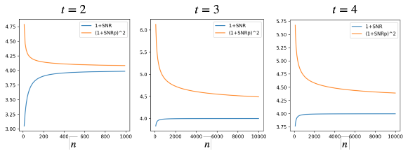
Figure 3: Plotting the gap between $1+\text{SNR}_{a}$ and $(1+\text{SNR}_{p})^{2}$ for the achievable scheme for $t=2,3,4$ and $N=t+1$. We vary $n$ from 10 to 10,000 and we observe that as $n$ grows the gap reduces.

8 Acknowledgement

This work is partially funded by the National Science Foundation under grants CAREER 1845852, FAI 2040880, CIF 1900750, 1763657, and 2231706..

Appendix A Finite precision analysis of the BGW coding scheme

Consider the BGW coding scheme where node $i$ gets - in a system with perfect precision - $\Gamma_{i}=p_{A}(x_{i}),\Theta_{i}=p_{B}(x_{i})$ for $i=1,2,\ldots,2t+1$, where:

$$p_{A}(x)=A+R_{1}x+R_{2}x^{2}+\ldots+R_{t}x^{t}$$

$$p_{B}(x)=B+S_{1}x+S_{2}x^{2}+\ldots+S_{t}x^{t}$$

and $x_{1},x_{2},\ldots,x_{2t+1}$ are distinct scalars. The DP parameter $\epsilon$ can be driven as close to $0$ as we wish by making $x_{1},x_{2},\ldots,x_{2t+1}$ arbitrarily large. In a system with perfect precision, node $i$ outputs $\Gamma_{i}\Theta_{i}$, and the decoder obtains $\widehat{C}=AB$ with perfect accuracy as a linear combination:

$$AB=\sum_{i=1}^{2t+1}d_{i}\Gamma_{i}\Theta_{i}$$ (1.80)

Similar to Section 6, we assume a system with finite precision where node $i$ receives:

$$\hat{\Gamma}_{i}=p_{A}(x_{i})+Y_{i}$$

$$\hat{\Theta}_{i}=p_{B}(x_{i})+Z_{i}$$

where $Y_{i}$ is a random variable that is independent of $\Gamma_{i}|_{i=1}^{2t+1}$,$\Theta_{i}|_{i=1}^{2t+1}$, $Z_{i}|_{i=1}^{2t+1}$, $\{Y_{j}:j\in\{1,2,\ldots,2t+1\}-\{i\}\}.$ Similarly $Z_{i}$ is a random variable that is independent of $\Gamma_{i}|_{i=1}^{2t+1}$,$\Theta_{i}|_{i=1}^{2t+1}$, $Y_{i}|_{i=1}^{2t+1}$, $\{Z_{j}:j\in\{1,2,\ldots,2t+1\}-\{i\}\}.$ Note that this independence property is achieved via dithered lattice quantizers as in Section 6. Node $i$ is assumed to output $\hat{\Gamma}_{i}\hat{\Theta}_{i}$ perfectly. Similarly to the reasoning in Section 6, we get $\mathbb{E}[Y_{i}^{2}],\mathbb{E}[Z_{i}^{2}]=\Omega(2^{-2M}),$ where $M$ is the number of bits of precision at each node. We assume that the decoder obtains:

$$\hat{C}=\sum_{i=1}^{2t+1}d_{i}\hat{\Gamma}_{i}\hat{\Theta}_{i}$$

where co-efficients $d_{i}$ are as in (1.80). We show next that choosing $M(\delta)=K\log\left(\frac{1}{\delta}\right)$ for any $K>0.5$ suffices to ensure that $\mathbb{E}[(AB-\hat{C})^{2}]\leq\delta$ for sufficiently small delta.

$$\mathbb{E}[(AB-\hat{C})^{2}]$$

$$=\mathbb{E}[(AB-\sum_{i=1}^{2t+1}d_{i}\hat{\Gamma}_{i}\hat{\Theta}_{i})^{2}]$$

$$=\mathbb{E}[(AB-\sum_{i=1}^{2t+1}d_{i}(\Gamma_{i}+Y_{i})(\Theta_{i}+Z_{i}))^{2}]$$

$$=\mathbb{E}[(AB-\sum_{i=1}^{2t+1}d_{i}\Gamma_{i}\Theta_{i})^{2}]+\Theta(2^{-2M(\delta)})$$

$$=0+\Theta(2^{-2M(\delta)})$$

Clearly, if $M(\delta)=K\log\left(\frac{1}{\delta}\right)$ for any $K>0.5,$ we have, for sufficiently small $\delta,$ $\mathbb{E}[(AB-\hat{C})^{2}]\leq\delta$ as required.

References

• [1] C.ย Dwork, F.ย McSherry, K.ย Nissim, and A.ย Smith, โ€œCalibrating noise to sensitivity in private data analysis,โ€ in Theory of Cryptography: Third Theory of Cryptography Conference, TCC 2006, New York, NY, USA, March 4-7, 2006. Proceedings 3.ย ย ย Springer, 2006, pp. 265โ€“284.
• [2] C.ย Dwork and A.ย Roth, โ€œThe algorithmic foundations of differential privacy,โ€ Foundations and Trendsยฎ in Theoretical Computer Science, vol.ย 9, no. 3โ€“4, pp. 211โ€“407, 2014. [Online]. Available: http://dx.doi.org/10.1561/0400000042
• [3] M.ย Ben-Or, S.ย Goldwasser, and A.ย Wigderson, โ€œCompleteness theorems for non-cryptographic fault-tolerant distributed computation,โ€ in Proceedings of the Twentieth Annual ACM Symposium on Theory of Computing, ser. STOC โ€™88.ย ย ย New York, NY, USA: Association for Computing Machinery, 1988, p. 1โ€“10. [Online]. Available: https://doi.org/10.1145/62212.62213
• [4] D.ย Evans, V.ย Kolesnikov, and M.ย Rosulek, โ€œA pragmatic introduction to secure multi-party computation,โ€ Foundations and Trendsยฎ in Privacy and Security, vol.ย 2, no. 2-3, 2017.
• [5] A.ย Shamir, โ€œHow to share a secret,โ€ Communications of the ACM, vol.ย 22, no.ย 11, pp. 612โ€“613, 1979.
• [6] Q.ย Yu, S.ย Li, N.ย Raviv, S.ย M.ย M. Kalan, M.ย Soltanolkotabi, and S.ย A. Avestimehr, โ€œLagrange coded computing: Optimal design for resiliency, security, and privacy,โ€ in The 22nd International Conference on Artificial Intelligence and Statistics.ย ย ย PMLR, 2019, pp. 1215โ€“1225.
• [7] C.ย Dwork, N.ย Kohli, and D.ย Mulligan, โ€œDifferential privacy in practice: Expose your epsilons!โ€ Journal of Privacy and Confidentiality, vol.ย 9, no.ย 2, 2019.
• [8] H.ย B. McMahan, G.ย Andrew, U.ย Erlingsson, S.ย Chien, I.ย Mironov, N.ย Papernot, and P.ย Kairouz, โ€œA general approach to adding differential privacy to iterative training procedures,โ€ arXiv preprint arXiv:1812.06210, 2018.
• [9] โ€œTensorflow privacy.โ€ [Online]. Available: https://www.tensorflow.org/responsible_ai/privacy/guide
• [10] N.ย Agarwal and K.ย Singh, โ€œThe price of differential privacy for online learning,โ€ in International Conference on Machine Learning.ย ย ย PMLR, 2017, pp. 32โ€“40.
• [11] J.ย C. Duchi, M.ย I. Jordan, and M.ย J. Wainwright, โ€œLocal privacy and statistical minimax rates,โ€ in 2013 IEEE 54th Annual Symposium on Foundations of Computer Science.ย ย ย IEEE, 2013, pp. 429โ€“438.
• [12] S.ย Asoodeh, M.ย Aliakbarpour, and F.ย P. Calmon, โ€œLocal differential privacy is equivalent to contraction of $e_{\gamma}$-divergence,โ€ arXiv preprint arXiv:2102.01258, 2021.
• [13] T.ย Stevens, C.ย Skalka, C.ย Vincent, J.ย Ring, S.ย Clark, and J.ย Near, โ€œEfficient differentially private secure aggregation for federated learning via hardness of learning with errors,โ€ in 31st USENIX Security Symposium (USENIX Security 22), 2022, pp. 1379โ€“1395.
• [14] S.ย Yuan, M.ย Shen, I.ย Mironov, and A.ย C.ย A. Nascimento, โ€œPractical, label private deep learning training based on secure multiparty computation and differential privacy,โ€ Cryptology ePrint Archive, Report 2021/835, 2021. [Online]. Available: https://ia.cr/2021/835
• [15] M.ย Pettai and P.ย Laud, โ€œCombining differential privacy and secure multiparty computation,โ€ in Proceedings of the 31st Annual Computer Security Applications Conference, ser. ACSAC 2015.ย ย ย New York, NY, USA: Association for Computing Machinery, 2015, p. 421โ€“430. [Online]. Available: https://doi.org/10.1145/2818000.2818027
• [16] X.ย He, A.ย Machanavajjhala, C.ย Flynn, and D.ย Srivastava, โ€œComposing differential privacy and secure computation: A case study on scaling private record linkage,โ€ in Proceedings of the 2017 ACM SIGSAC Conference on Computer and Communications Security, ser. CCS โ€™17.ย ย ย New York, NY, USA: Association for Computing Machinery, 2017, p. 1389โ€“1406. [Online]. Available: https://doi.org/10.1145/3133956.3134030
• [17] J.ย Bรถhler and F.ย Kerschbaum, โ€œSecure multi-party computation of differentially private median,โ€ in 29th USENIX Security Symposium (USENIX Security 20).ย ย ย USENIX Association, Aug. 2020, pp. 2147โ€“2164. [Online]. Available: https://www.usenix.org/conference/usenixsecurity20/presentation/boehler
• [18] A.ย Royย Chowdhury, C.ย Wang, X.ย He, A.ย Machanavajjhala, and S.ย Jha, โ€œCrypt$\epsilon$: Crypto-assisted differential privacy on untrusted servers,โ€ in Proceedings of the 2020 ACM SIGMOD International Conference on Management of Data, ser. SIGMOD โ€™20.ย ย ย New York, NY, USA: Association for Computing Machinery, 2020, p. 603โ€“619. [Online]. Available: https://doi.org/10.1145/3318464.3380596
• [19] K.ย Talwar, โ€œDifferential secrecy for distributed data and applications to robust differentially secure vector summation,โ€ arXiv preprint arXiv:2202.10618, 2022.
• [20] Q.ย Yu, S.ย Li, N.ย Raviv, S.ย M.ย M. Kalan, M.ย Soltanolkotabi, and S.ย A. Avestimehr, โ€œLagrange coded computing: Optimal design for resiliency, security, and privacy,โ€ in Proceedings of the Twenty-Second International Conference on Artificial Intelligence and Statistics, vol.ย 89, 2019, pp. 1215โ€“1225. [Online]. Available: https://proceedings.mlr.press/v89/yu19b.html
• [21] M.ย Soleymani, H.ย Mahdavifar, and A.ย S. Avestimehr, โ€œAnalog lagrange coded computing,โ€ IEEE Journal on Selected Areas in Information Theory, vol.ย 2, no.ย 1, pp. 283โ€“295, 2021. [Online]. Available: https://doi.org/10.1109/JSAIT.2021.3056377
• [22] H.ย Akbari-Nodehi and M.ย A. Maddah-Ali, โ€œSecure coded multi-party computation for massive matrix operations,โ€ IEEE Transactions on Information Theory, vol.ย 67, no.ย 4, pp. 2379โ€“2398, 2021.
• [23] W.-T. Chang and R.ย Tandon, โ€œOn the capacity of secure distributed matrix multiplication,โ€ in 2018 IEEE Global Communications Conference (GLOBECOM), 2018, pp. 1โ€“6.
• [24] R.ย G.ย L. Dโ€™Oliveira, S.ย Elย Rouayheb, and D.ย Karpuk, โ€œGasp codes for secure distributed matrix multiplication,โ€ IEEE Transactions on Information Theory, vol.ย 66, no.ย 7, pp. 4038โ€“4050, 2020.
• [25] Z.ย Jia and S.ย A. Jafar, โ€œOn the capacity of secure distributed batch matrix multiplication,โ€ IEEE Transactions on Information Theory, vol.ย 67, no.ย 11, pp. 7420โ€“7437, 2021.
• [26] Z.ย Chen, Z.ย Jia, Z.ย Wang, and S.ย A. Jafar, โ€œGcsa codes with noise alignment for secure coded multi-party batch matrix multiplication,โ€ IEEE Journal on Selected Areas in Information Theory, vol.ย 2, no.ย 1, pp. 306โ€“316, 2021.
• [27] M.ย Fahim and V.ย R. Cadambe, โ€œNumerically stable polynomially coded computing,โ€ IEEE Transactions on Information Theory, vol.ย 67, no.ย 5, pp. 2758โ€“2785, 2021.
• [28] Q.ย Geng and P.ย Viswanath, โ€œThe optimal noise-adding mechanism in differential privacy,โ€ IEEE Transactions on Information Theory, vol.ย 62, no.ย 2, pp. 925โ€“951, 2016. [Online]. Available: https://doi.org/10.1109/TIT.2015.2504967
• [29] Q.ย Geng, W.ย Ding, R.ย Guo, and S.ย Kumar, โ€œTight analysis of privacy and utility tradeoff in approximate differential privacy,โ€ in Proceedings of the Twenty Third International Conference on Artificial Intelligence and Statistics, vol. 108.ย ย ย PMLR, 26โ€“28 Aug 2020, pp. 89โ€“99. [Online]. Available: https://proceedings.mlr.press/v108/geng20a.html
• [30] P.ย Kairouz, S.ย Oh, and P.ย Viswanath, โ€œSecure multi-party differential privacy,โ€ in Advances in Neural Information Processing Systems, vol.ย 28, 2015.
• [31] โ€”โ€”, โ€œDifferentially private multi-party computation,โ€ in 2016 Annual Conference on Information Science and Systems (CISS), 2016, pp. 128โ€“132. [Online]. Available: https://doi.org/10.1109/CISS.2016.7460489
• [32] D.ย Guo, โ€œMutual information and minimum mean-square error in gaussian channels,โ€ IEEE transactions on information theory, vol.ย 51, no.ย 4, pp. 1261โ€“1282, 2005.
• [33] R.ย Zamir, Lattice Coding for Signals and Networks: A Structured Coding Approach to Quantization, Modulation, and Multiuser Information Theory.ย ย ย Cambridge University Press, 2014.
• [34] H.ย Jeong, A.ย Devulapalli, V.ย R. Cadambe, and F.ย P. Calmon, โ€œฯตitalic-ฯต\epsilon-approximate coded matrix multiplication is nearly twice as efficient as exact multiplication,โ€ IEEE Journal on Selected Areas in Information Theory, vol.ย 2, no.ย 3, pp. 845โ€“854, 2021. [Online]. Available: https://doi.org/10.1109/JSAIT.2021.3099811
• [35] J.ย Wang, Z.ย Jia, and S.ย A. Jafar, โ€œPrice of precision in coded distributed matrix multiplication: A dimensional analysis,โ€ in 2021 IEEE Information Theory Workshop (ITW).ย ย ย IEEE, 2021, pp. 1โ€“6.
• [36] G.ย Bresler, A.ย Parekh, and N.ย David, โ€œThe approximate capacity of the many-to-one and one-to-many gaussian interference channels,โ€ IEEE Transactions on Information Theory, vol.ย 56, no.ย 9, pp. 4566โ€“4592, 2010.
• [37] S.ย A. Jafar and S.ย Vishwanath, โ€œGeneralized degrees of freedom of the symmetric gaussian $k$ user interference channel,โ€ IEEE Transactions on Information Theory, vol.ย 56, no.ย 7, pp. 3297โ€“3303, 2010.
• [38] C.ย Huang, V.ย R. Cadambe, and S.ย A. Jafar, โ€œInterference alignment and the generalized degrees of freedom of the $ X $ channel,โ€ IEEE Transactions on Information Theory, vol.ย 58, no.ย 8, pp. 5130โ€“5150, 2012.
• [39] U.ย Niesen and M.ย A. Maddah-Ali, โ€œInterference alignment: From degrees of freedom to constant-gap capacity approximations,โ€ IEEE Transactions on Information Theory, vol.ย 59, no.ย 8, pp. 4855โ€“4888, 2013.