Geometrically Local Quantum and Classical Codes from Subdivision

Abstract

A geometrically local quantum code is an error correcting code situated within $\mathbb{R}^{D}$, where the checks only act on qubits within a fixed spatial distance. The main question is: What is the optimal dimension and distance for a geometrically local code? This question was recently answered by Portnoy which constructed codes with optimal dimension and distance up to polylogs. This paper extends Portnoy’s work by constructing a code which additionally has an optimal energy barrier up to polylogs. The key ingredient is a simpler code construction obtained by subdividing the balanced product codes. We also discuss applications to classical codes.

1 Introduction

Coding theory has been the center of many applications and is especially important in quantum computing to maintain quantum coherence under noise. One particular focus is on quantum codes whose parity-checks only act on a few qubits, also known as the quantum low-density parity-check (qLDPC) codes. The LDPC property is favorable for quantum codes because quantum information is highly sensitive to noise and measurements often cause errors. The fewer the qubits involved, the lower the measurement error. This is in sharp contrast to practical classical codes which suffer from essentially no measurement error. Finding qLDPC codes with large distance and dimension has been an important open question in coding theory; it is only recently that such codes have been constructed [1].

However, for certain applications, having low density is not enough. Since we live in a three dimensional world, the code should be embedded in $\mathbb{R}^{3}$. We want each check to be implementable via short range measurements and we want the qubit density to be finite. Such codes are called geometrically local.

Finding geometrically local codes with large distance and dimension has also been an important question for physicists and coding theorists. Back in 2008, Bravyi and Terhal [2] showed an upper bound on code distance and in 2009, Bravyi, Poulin, and Terhal [3] extended the previous result to an upper bound on the tradeoff between code dimension and code distance. At the time, the only known geometrically local codes were the high-dimensional toric codes, which saturate the upper bound in two dimensions, but not in higher dimensions. As such, it was thought that this upper bound is not tight and can be improved. However, Haah in 2011 [4] and Michnicki in 2012 [5] constructed new geometrically local codes that beat the toric codes, thus improving the lower bound. Despite these advancements, the gap between the upper and lower bounds remained open.

Recently, Portnoy [6] finally closes the gap up to polylogs. The idea is to take the good qLDPC codes mentioned earlier, “geometrize” the codes, turning them into manifolds based on the results of Freedman and Hastings [7], and finally embed the manifolds into $\mathbb{R}^{D}$ using the work of Gromov and Guth [8]. It is remarkable how the construction takes a code to geometry and then back to code again.

However, one unsatisfactory aspect is that the step that turns codes into manifolds is somewhat complicated. In this paper, we circumvent this step by utilizing the structure of the good qLDPC codes people have constructed in a non-black box manner. In particular, the structure we will use is the balanced product introduced in [9]. As a result, our code construction is more explicit. To demonstrate this advantage, we show that our code additionally has the optimal energy barrier (up to polylogs).

1.1 Main Contribution

Our main contribution is to identify a 2d geometrical structure for the balanced product codes. This enables us to simplify the previous construction [6] by avoiding the step that turns codes into manifolds. Our code gives the optimal distance and energy barrier.

Theorem 1.1.

There exists a family of $D$-dimensional geometrically local quantum codes ($D\geq 3$) with code dimension $k=\Omega(n^{\frac{D-2}{D}}/\operatorname{polylog}(n))$, distance $d=\Omega(n^{\frac{D-1}{D}}/\operatorname{polylog}(n))$, and energy barrier $\mathcal{E}=\Omega(n^{\frac{D-2}{D}}/\operatorname{polylog}(n))$.

Remark 1.2.

After learning about Baspin and Williamson’s work where they achieved optimal distance without a loss of polylog factor, we noticed that we can also remove the polylog factor by constructing an optimal embedding of a particular expander graph in $\mathbb{R}^{D}$. This construction will be described in a future paper.

As a result, we obtain an explicit family of optimal $D$-dimensional geometrically local quantum codes with code dimension $k=\Omega(n^{\frac{D-2}{D}})$, distance $d=\Omega(n^{\frac{D-1}{D}})$, and energy barrier $\mathcal{E}=\Omega(n^{\frac{D-2}{D}})$. The same method for removing polylogs is applicable to all the cases below as well.

This answers the questions raised in Portnoy’s work [6]. We answer Question 2 affirmatively and show that we can bypass the manifolds (at least for some good qLDPC codes). Moreover, our code likely has a decoder based on surface codes which potentially resolves Question 3. For Question 1, as discussed in Remark 1.2, it is possible to remove the polylog factors by constructing an explicit embedding of the expander graph which will be discussed in a future paper.

Besides these results on geometrically local quantum codes, by applying the same idea, we obtain geometrically local classical codes with optimal distance, and energy barrier. Additionally, this code has nontrivial soundness.

Theorem 1.3.

There exists a family of $D$-dimensional geometrically local classical codes ($D\geq 2$) with code dimension $k=\Omega(n^{\frac{D-1}{D}}/\operatorname{polylog}(n))$, distance $d=\Omega(n/\operatorname{polylog}(n))$, energy barrier $\mathcal{E}=\Omega(n^{\frac{D-1}{D}}/\operatorname{polylog}(n))$, and soundness $s=\Omega(n^{-\frac{1}{D}}/\operatorname{polylog}(n))$.

As a consequence of the codes above, we obtain codes that saturate the tradeoff between code dimension and distance. This is achieved by copying the codes multiple times and stacking them into a grid. In particular, one can construct a new family of codes of size $L^{D}$ by stacking $a^{D}$ many codes, as described above, each of size $(L/a)^{D}$. By choosing suitable values for $a$, we obtain the following code families.

Corollary 1.4.

There exists a family of $D$-dimensional geometrically local quantum codes ($D\geq 3$) with code dimension $k\geq\Omega(n^{\frac{D-2}{D}}/\operatorname{polylog}(n))$, distance $d=\Omega((n/k)^{\frac{D-1}{2}}/\operatorname{polylog}(n))$, and energy barrier $\mathcal{E}=\Omega((n/k)^{\frac{D-2}{2}}/\operatorname{polylog}(n))$.

Corollary 1.5.

There exists a family of $D$-dimensional geometrically local classical codes ($D\geq 2$) with code dimension $k\geq\Omega(n^{\frac{D-1}{D}}/\operatorname{polylog}(n))$, distance $d=\Omega((n/k)^{D}/\operatorname{polylog}(n))$, energy barrier $\mathcal{E}=\Omega((n/k)^{D-1}/\operatorname{polylog}(n))$, and soundness $s=\Omega((n/k)^{-1}/\operatorname{polylog}(n))$.

As discussed in Appendix A, $D$-dimensional geometrically local quantum codes satisfy $d=O((n/k)^{\frac{D-1}{2}})$ and the $D$-dimensional geometrically local classical codes satisfy $d=O((n/k)^{D})$. Therefore, the codes above saturate the tradeoff between code dimension and distance (up to polylogs). Whether the tradeoff between code dimension and energy barrier is optimal is left as an open question.

Furthermore, our construction method readily generalizes to other settings, including codes derived from cubical complexes and local Hamiltonians beyond codes, although their properties require further investigation.

1.2 Construction and Proof Overview

One of the difficulties in constructing geometrically local codes is that good qLDPC codes are geometrically non-local. This is because good qLDPC codes are based on expander graphs which do not have geometrically local embeddings. Nevertheless, we can still force an embedding by paying the cost that the vertices in the graph are far apart. If one continues this thought, a way to get a graph with a local embedding is to insert new vertices on each long range edge, subdividing them into constant sized edges. This gives a graph which is geometrically local yet retains some of the expansion properties. A similar idea applies to good classical LDPC codes whose parity-check matrix corresponds to the adjacency matrix of a bipartite graph. This procedure gives a geometrically local classical code with the optimal dimension and distance.

We essentially apply the same idea to quantum LDPC codes. Many of the known good qLDPC codes can be phrased in terms of a balanced product. The balanced product codes may be obtained by taking a certain product of two classical code. To embed the resulting complex in $\mathbb{R}^{D}$, all we need to do is to subdivide each edge and face by adding vertices. The subdivision process is illustrated in Figure 1.

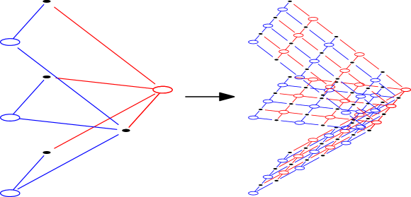
Figure 1: The subdivision of a balanced product code. Blue circles, black dots and red circles represent X - stabilisers, qubits and Z - stabilisers, respectively.

The proof mainly involves properties of the chain map $\mathcal{F}$, which maps from $\mathbb{F}_{2}^{X(0)}\to\mathbb{F}_{2}^{X(1)}\to\mathbb{F}_{2}^{X(2)}$, the chain complex of the original good qLDPC code, to $\mathbb{F}_{2}^{X_{L}(0)}\to\mathbb{F}_{2}^{X_{L}(1)}\to\mathbb{F}_{2}^{X_{L}(2)}$, the chain complex of the subdivided code.

(1)

The strategy to show any desired property in $X_{L}$, say distance, is to reduce to the same property in $X$. This reduction relies on codes that are similar to the surface code and the repetition code that arise naturally when we perform the subdivision. We call these the generalized surface codes and the generalized repetition codes, as illustrated in Figure 2. One intuition is that the subdivided code is a concatenated code with the inner code being the generalized surface and repetition codes and the outer code being the good qLDPC code.

Figure 2: The generalized surface code and generalized repetition code.

1.3 Related Work

Good qLDPC codes

Our result relies heavily on the recent progress of good qLDPC codes. We summarize some recent advances. One main open question in quantum coding theory was whether qLDPC codes with linear distance and dimension exist. The earliest qLDPC codes are Kitaev’s toric codes and surface codes [10] with dimension $k=\Theta(1)$ and distance $d=\Theta(\sqrt{n})$. Progress in the field led to the discovery of codes with improved rates $k=\Theta(n)$ [11] and better distances $d=\Theta(\textnormal{polylog}(n)\sqrt{n})$ [12, 13, 14]. A significant breakthrough occurred when [15] improved the distance by a polynomial factor and broke the square root barrier. Following works achieved nearly linear distance $d=\Theta(n/\log n)$ [16] and discovered the framework of balanced product and derandomized the earlier construction [9]. Finally, [1] showed the existence of good quantum LDPC codes with $k=\Theta(n)$ and $d=\Theta(n)$. Subsequently, two more constructions were discovered [17, 18]. All these codes were shown to have a linear time sequential decoder [19, 20, 18] and a log time parallel decoder [21]. Besides coding theory, these codes also have applications in complexity theory [22], notably in resolving the NLTS conjecture [23].

Geometrically Local Quantum Codes

As we live in a three-dimensional world, it is natural to explore codes that can be embedded in 3d, with the potential realization physical materials. This exploration also extends to codes that can be embedded in higher dimensions. We first discuss the lower bound of the parameters for the local quantum codes then we discuss the upper bound.

The earliest local quantum code studied was the generalized toric code [24]. The code is constructed by subdividing the $D=D_{1}+D_{2}$ dimensional torus into grids of size $L^{D}$. Subsequently, qubits are placed on $D_{1}$-cells, X-checks on $(D_{1}-1)$-cells, and Z-checks on $(D_{1}+1)$-cells. Since the torus has nontrivial $D_{1}$-homology, the code is nontrivial with dimension $\Theta(1)$. Additionally, since the nontrivial X (Z) logical operator corresponds to a $D_{2}$ ($D_{1}$) dimensional surface, one can show that the code has X-distance $\Theta(L^{D_{2}})=\Theta(n^{\frac{D_{2}}{D}})$ and Z-distance $\Theta(L^{D_{1}})=\Theta(n^{\frac{D_{1}}{D}})$ where $n=\Theta(L^{D})$ is the number of qubits. In physics, this code is also known as the $\mathbb{Z}_{2}$ gauge theory which is a topological quantum field theory (TQFT). Codes from TQFT were the best codes known at the time. As a comparison to the codes that will be described later, the 3d toric code has parameters $[[n=\Theta(L^{3}),k=\Theta(1),d=\Theta(L),\mathcal{E}=\Theta(1)]]$.

To obtain better codes, we have to go beyond TQFT. In particular, two novel code constructions appeared. One was by Haah in 2011 [4] which constructed the first 3d gapped Hamiltonian beyond TQFT. This code has parameters $[[n=\Theta(L^{3}),k=\Theta(L),d=\Omega(L^{\gamma}),\mathcal{E}=\Omega(\log L)]]$ for some $\gamma>1$ [25]. In particular, it has superlinear distance and non constant energy barrier. This breakthrough not only changes our understand of local quantum codes, but also spark the nascent field of fractons in condensed matter physics.

Haah discovered the code by asking whether a 3d lattice code could exist without string operators, which is a characteristic property of TQFTs. He observed that lattice codes in 3d with translation invariance can be compactly described as modules over the polynomial ring $\mathbb{F}_{2}[x,y,z]$. He then rephrased the no-string rule as a property in commutative algebra and discovered this nontrivial code.

The other construction was introduced by Michnicki in 2012 [5]. The new technique, known as “welding”, involves welding together surface codes along the edges to form a larger code. (In fact, our code can also be viewed as a welded code, using good qLDPC codes as a guide for the welding process.) The code has parameters $[[n=\Theta(L^{3}),k=1,d=\Theta(L^{\frac{4}{3}}),\mathcal{E}=\Theta(L^{\frac{2}{3}})]]$. In particular, it has a polynomial energy barrier. Notably, this is the first geometrically local quantum code that does not have translation invariance.

The most recent code by Portnoy in 2023 [6] has parameters $[[n=\Theta(L^{3}),k=\Omega(L/\operatorname{polylog}L),d=\Omega(L^{2}/\operatorname{polylog}L)]]$. In our work, we extend the parameters to include the energy barrier $[[n=\Theta(L^{3}),k=\Omega(L/\operatorname{polylog}L),d=\Omega(L^{2}/\operatorname{polylog}L),\mathcal{E}=\Omega(L/\operatorname{polylog}L)]]$.

Besides the question on local quantum codes, one can also ask about local classical code. The work by Yoshida in 2011 [26] constructed local classical codes based on fractals. This achieves the optimal scaling between code dimension and distance $[n=\Theta(L^{D}),k=\Omega(L^{D-1}/\operatorname{polylog}L),d=\Theta(L^{D}/\operatorname{polylog}L),\mathcal{E}=\Theta(\log L)]$. Our work improves the energy barrier and show that the code has nontrivial soundness $[[n=\Theta(L^{D}),k=\Omega(L^{D-1}/\operatorname{polylog}L),d=\Omega(L^{D}/\operatorname{polylog}L),\mathcal{E}=\Omega(L^{D-1}/\operatorname{polylog}L),s=\Omega(L^{-1}/\operatorname{polylog}L)]]$. We remark that quantum codes based on fractals have also been explored [27, 28], but either the embedding in 3d is unknown or the code does not have superlinear distance. This concludes the discussion on the lower bound.

The upper bound on distance and energy barrier for quantum and classical codes was studied in [2] and the tradeoff between code dimension and distance was studied in [3]. These imply that the optimal $D$ dimensional classical code has distance $\Theta(L^{D})$ and energy barrier $\Theta(L^{D-1})$. Under these conditions the optimal dimension is $\Theta(L^{D-1})$. Similarly, the optimal $D$ dimensional quantum code has distance $\Theta(L^{D-1})$ and energy barrier $\Theta(L^{D-2})$. Under these conditions the optimal dimension is $\Theta(L^{D-2})$. Specific results can be found in Appendix A.

On the other hand, through a different starting assumption, [29] showed that all quantum codes that have “homogeneous topological order” have upper bounds on the code dimension $k=O(L^{D-2})$. Notice that all the codes discussed above have homogeneous topological order.

1.4 Further Directions

Efficient Decoder?

Can we show the code discussed in this paper has an efficient decoder that decodes correctly up to a constant times the distance? It seems plausible this decoder could be obtained by combining the decoder for the surface code and the decoder for the original qLDPC code.

“Geometrize” Quantum Tanner Code by Leverrier and Zémor?

All known constructions of good qLDPC codes can be viewed as balanced product which induces a geometric embedding with the exception of the quantum Tanner code [17]. Can we induce a geometric embedding for the quantum Tanner code? We propose a possible construction in Appendix B.

Simpler Manifold Construction?

This paper bypasses Freedman, Hastings [7] by noticing balanced product codes naturally correspond to square complexes. Can we use this feature to construct a manifold corresponding to the balanced product code in a simpler way? Perhaps this leads to a lower dimensional manifold construction. See [7, Sec 1.9] for further context.

Geometric Embedding Beyond Codes?

This paper focuses on converting a qLDPC code into a geometrically local quantum code. We wonder if this reduction can be applied to other questions. For example, we know that the local Hamiltonian question is QMA-hard. Can we obtain a reduction to questions about geometrically local Hamiltonians? Or, the SYK model is given by the random 4-fermion Hamiltonian. Can we convert this into a geometrically local Hamiltonian? These questions can be posed in the context of both traditional classical CSP problems and quantum Hamiltonians.

Geometrically Local Codes with Translation Invariance?

This paper shows a matching upper and lower bound for distance and energy barrier of geometrically local codes. What if we additionally impose translation invariance? The code constructed by Haah in 3d of size $L\times L\times L$ was shown to have superlinear distance $\Omega(L^{\gamma})$ for some $\gamma>1$, and energy barrier $\Omega(\log L)$ by Bravyi and Haah [25]. Neither of these match the upper bound in [2]. Can we possibly close this gap?

Geometric Embedding in Fractals Geometries?

This paper achieves the optimal code dimension and distance in $\mathbb{Z}^{D}$. What about the optimal code in fractal geometries? Similar questions have been explored previously in [28].

Self-Correcting Quantum Memory?

Self-correcting quantum memories [24, 30, 31] are the quantum analog of magnetic tapes. Magnetic tapes are passive, non-volatile memories that can retain information for a long time without active error correction. A natural question is: Can we find geometrically local quantum codes in 3d with similar properties? It is known that 4d toric codes have this property [24, 30] and 2d stabilizer codes do not have this property [2]. However, it remains open whether 3d self-correcting quantum memories exist.

Note that even though our code has large energy barrier, we do not think our code is self-correcting. This is because our code utilizes the 2d toric code and probably shares similar thermal properties.

2 Preliminary

2.1 Chain Complexes

Chain complexes provide a natural framework for describing both quantum CSS codes and certain constructions of classical locally testable codes, which are the focus of this work. Later, we will see that many properties of the codes, including distance, energy barrier for quantum codes, and local testability for classical codes, can be interpreted in terms of expansion properties of the chain complex defined in Section 2.4.

Definition 2.1 (Chain complex).

A chain complex $X$ consists of a sequence of vector spaces $\mathbb{F}_{2}^{X(i)}$ generated by sets $X(i)$, along with linear maps $\delta_{i}:\mathbb{F}_{2}^{X(i)}\rightarrow\mathbb{F}_{2}^{X(i+1)}$ known as coboundary operators, where the coboundary operators satisfy

$$\delta_{i+1}\delta_{i}=0.$$

Given a chain complex, one can change the direction of the linear maps and form the dual chain complex consists of the boundary operators. In our context, there is a canonical basis of $\mathbb{F}_{2}^{X(i)}$ labeled by the elements of $X(i)$. Using this basis, we can define the associate boundary operators $\partial_{i}:\mathbb{F}_{2}^{X(i)}\rightarrow\mathbb{F}_{2}^{X(i-1)}$ as the matrix transpose of $\delta_{i-1}$, $\partial_{i}\coloneqq\delta_{i-1}^{T}$. The boundary operators automatically satisfy

$$\partial_{i-1}\partial_{i}=0$$

which is again a chain complex.

We introduce some standard terminologies. Elements of the kernel of the (co)boundary operators are called (co)-cycles

$$Z_{i}\coloneqq\operatorname{ker}\partial_{i}=\{c_{i}\in\mathbb{F}_{2}^{X(i)}:\partial_{i}c_{i}=0\},\qquad Z^{i}\coloneqq\operatorname{ker}\delta_{i}=\{c_{i}\in\mathbb{F}_{2}^{X(i)}:\delta_{i}c_{i}=0\}.$$

Elements of the image of the (co)boundary operators are called (co)boundaries

$$B_{i}\coloneqq\operatorname{im}\partial_{i+1}=\{\partial_{i+1}c_{i+1}:c_{i+1}\in\mathbb{F}_{2}^{X(i+1)}\},\qquad B^{i}\coloneqq\operatorname{im}\delta_{i-1}=\{\delta_{i-1}c_{i-1}:c_{i-1}\in\mathbb{F}_{2}^{X(i-1)}\}.$$

Because $\delta_{i}\delta_{i-1}=0$, it follows that $B^{i}\subset Z^{i}$. When $B^{i}=Z^{i}$ the chain complex is said to be exact at $i$.

2.2 Classical and Quantum Error Correcting Codes

2.2.1 Classical Error Correcting Codes

A classical code is a $k$-dimensional linear subspace $C\subset\mathbb{F}_{2}^{n}$ which is specified by a parity-check matrix $H:\mathbb{F}_{2}^{n}\to\mathbb{F}_{2}^{m}$ where $C=\operatorname{ker}H$. $n$ is called the size and $k$ is called the dimension. The distance $d$ is the minimum Hamming weight of a nontrivial codeword

$$d=\min_{c\in C-\{0\}}|c|.$$ (2)

The energy barrier $E$ is the minimum energy required to generate a nontrivial codeword by flipping the bits one at a time. More precisely, given a vector $c\in\mathbb{F}_{2}^{n}$, $|Hc|$ is the number of violated checks. In the physical context, the energy of a state is proportional to the number of violated checks, so we will refer to $\epsilon(c)=|Hc|$ as the energy of vector $c$. We say a sequence of vectors $\gamma_{a\to b}=(c_{0}=a,c_{1},...,c_{t}=b)$ is a walk from $a$ to $b$ if $c_{i},c_{i+1}$ differ by exactly one bit $|c_{i}-c_{i+1}|=1$. The energy of a walk $\epsilon(\gamma)=\max_{c_{i}\in\gamma}\epsilon(c_{i})$ is defined as the maximum energy reached among the vectors in $\gamma$. Finally, the energy barrier $\mathcal{E}$ is defined as the minimum energy among all walks $\gamma$ from $0$ to a nontrivial codeword

$$\mathcal{E}=\min_{\gamma_{0\to c},c\in C-\{0\}}\epsilon(\gamma_{0\to c}).$$ (3)

Intuitively, energy barrier is another way to characterize the difficulty for a logical error to occur, other than distance.

We say the classical code is a low-density parity-check (LDPC) code if each check interacts with a bounded number of bits, i.e. $H$ has a bounded number of nonzero entries in each row.

We say the classical code is (strongly) locally testable with soundness $s$ if it satisfies

$$\forall x\in\mathbb{F}_{2}^{n}:\frac{1}{m}|Hx|\geq\frac{s}{n}\min_{c\in C}|x-c|.$$ (4)

Notice that if the code has large distance and soundness then the code has large energy barrier where $\mathcal{E}\geq s\frac{m}{n}\frac{d}{2}=\Theta(sd)$. The reason is that if $\epsilon(x)=|Hx|<s\frac{m}{n}\frac{d}{2}$, by soundness, $\min_{c\in C}|x-c|<d/2$. Therefore, a walk $\gamma$ starting from $0$ with energy $<s\frac{m}{n}\frac{d}{2}$ cannot reach other codewords. Hence, $\mathcal{E}\geq s\frac{m}{n}\frac{d}{2}$.

2.2.2 Quantum CSS Codes

A quantum CSS code is specified by two classical codes $C_{x},C_{z}$ represented by their parity-check matrices $H_{x}:\mathbb{F}_{2}^{n}\to\mathbb{F}_{2}^{m_{z}},H_{z}:\mathbb{F}_{2}^{n}\to\mathbb{F}_{2}^{m_{x}}$ which satisfy $H_{x}H_{z}^{T}=0$. $n$, $m_{x}$, and $m_{z}$ are the number of qubits, the number of $X$ and $Z$ checks (i.e. stabilizer generators), respectively. The code consists of $X$ and $Z$ logical operators represented by $C_{x}$ and $C_{z}$, $X$ and $Z$ stabilizers represented by $C_{z}^{\perp}$ and $C_{x}^{\perp}$, and nontrivial $X$ and $Z$ logical operators represented by $C_{x}-C_{z}^{\perp}$ and $C_{z}-C_{x}^{\perp}$. The dimension $k=\dim C_{x}-\dim C_{z}^{\perp}$ is the number of logical qubits. The distance is $d=\min(d_{x},d_{z})$ where

$$d_{x}=\min_{c_{x}\in C_{x}-C_{z}^{\perp}}|c_{x}|,\qquad d_{z}=\min_{c_{z}\in C_{z}-C_{x}^{\perp}}|c_{z}|$$ (5)

are called the $X$ and $Z$ distance which are the minimal weights of the nontrivial $X$ and $Z$ logical operators. The energy barrier is $\mathcal{E}=\min(\mathcal{E}_{x},\mathcal{E}_{z})$ where $\mathcal{E}_{x}$ and $\mathcal{E}_{z}$ are the minimum energy required to create a nontrivial $X$ and $Z$ logical operator

$$\mathcal{E}_{x}=\min_{\gamma_{0\to c_{x}},c_{x}\in C_{x}-C_{z}^{\perp}}\epsilon_{x}(\gamma_{0\to c_{x}}),\qquad\mathcal{E}_{z}=\min_{\gamma_{0\to c_{z}},c_{z}\in C_{z}-C_{x}^{\perp}}\epsilon_{z}(\gamma_{0\to c_{z}}),$$ (6)

where $\epsilon_{x}(c_{x})=|H_{x}c_{x}|$ is the number of violated $Z$-checks of the $X$ Pauli operator $c_{x}$ and $\epsilon_{z}(c_{z})=|H_{z}c_{z}|$ is the number of violated $X$-checks of the $Z$ Pauli operator $c_{z}$.

We say the quantum code is a low-density parity-check (LDPC) code if each check interacts with a bounded number of qubits and each qubit interacts with bounded number of checks, i.e. $H_{x}$ and $H_{z}$ have bounded number of nonzero entries in each column and row.

We remark that a quantum CSS code naturally corresponds to a chain complex. In particular, $H_{x}$ and $H_{z}$ induce the chain complex

$$X:\mathbb{F}_{2}^{m_{x}}\xrightarrow{\delta_{0}=H_{z}^{T}}\mathbb{F}_{2}^{n}\xrightarrow{\delta_{1}=H_{x}}\mathbb{F}_{2}^{m_{z}}.$$ (7)

In reverse, a chain complex also defines a quantum CSS code. We denote the corresponding quantum code as $Q(X)$. Later on, $X$ will mainly stands for the chain complex and not the $X$ in $X$-check.

2.2.3 Geometric Properties: Geometrically Local and Bounded Density

In addition to the linear algebraic structure from the parity-check matrices, the codes studied in this paper additionally have geometric structures. In particular, the code is embedded in $\mathbb{Z}^{D}$ where each bit/qubit and check has a corresponding location in $\mathbb{Z}^{D}$

$$I_{\textnormal{code}\to\textnormal{euclid}}:\operatorname{Set}(C)\to\mathbb{Z}^{D}\quad\text{or}\quad\operatorname{Set}(Q)\to\mathbb{Z}^{D},$$ (8)

where $\operatorname{Set}(C)$ and $\operatorname{Set}(Q)$ are the sets that label the bits/qubits and the checks. For classical codes $\operatorname{Set}(C)=[n]\sqcup[m]$ and for quantum codes $\operatorname{Set}(Q)=[m_{x}]\sqcup[n]\sqcup[m_{z}]$, where $[n]$ is a set of size $n$ which labels the basis vectors of $\mathbb{F}_{2}^{n}$ and $\sqcup$ is the disjoint union.

We say the embedding is $a$-geometrically-local if the Euclidean distance between each check and the qubit it interacts with is $\leq a$. That is, if $H_{ij}$ is nonzero, then $|I_{\textnormal{code}\to\textnormal{euclid}}(i)-I_{\textnormal{code}\to\textnormal{euclid}}(j)|\leq a$ where $|\cdot|$ is the Euclidean distance. We say the embedding has density $b$ if the number of qubits and checks located at each lattice point in $\mathbb{Z}^{D}$ is $\leq b$. The goal is to have constant parameters $a=\Theta(1)$, $b=\Theta(1)$.

2.3 Good Quantum LDPC Code and Good Classical LTC from Balanced Product

We now extract and review the key features of the good quantum LDPC codes constructed in [1, 32, 18] that allow us to transform them into geometrically local codes. While each paper has its preferred way of describing their construction, here, we will put all of them under the umbrella of the balanced product [9] (also known as $G$-lifted product in [1]), since it is the structure that allows us to put the code on a 2d square complex in a simple way. We will start by reviewing the balanced product construction, then discuss how the above good codes can be viewed as a balanced product code.

2.3.1 Balanced Product of Codes

Given two codes with invariant group actions $G$, the associated balanced product code is the tensor product of the two codes quotiented by the diagonal group action. More precisely, let $H_{A}:\mathbb{F}_{2}^{X_{A}(0)}\to\mathbb{F}_{2}^{X_{A}(1)}$ and $H_{B}:\mathbb{F}_{2}^{X_{B}(0)}\to\mathbb{F}_{2}^{X_{B}(1)}$ be the parity-check matrices of the two codes. The group $G$ act on sets $X_{A}(0),X_{A}(1),X_{B}(0),X_{B}(1)$ such that $H_{A}$ and $H_{B}$ are invariant, i.e. $\langle\widehat{a}_{1},H_{A}\widehat{a}_{0}\rangle=\langle\widehat{ga_{1}},H_{A}\widehat{ga_{0}}\rangle$ where $\widehat{a}_{0}$ ($\widehat{a}_{1}$) is a basis vector labeled by an element $a_{0}\in X_{A}(0)$ ($a_{1}\in X_{A}(1)$) and $\langle\cdot,\cdot\rangle$ is the inner product. This implies an invariant group action of $G\times G$ on $H_{A}\otimes H_{B}:\mathbb{F}_{2}^{X_{A}(0)\times X_{B}(0)}\xrightarrow{\delta_{0}}\mathbb{F}_{2}^{X_{A}(1)\times X_{B}(0)\cup X_{A}(0)\times X_{B}(1)}\xrightarrow{\delta_{1}}\mathbb{F}_{2}^{X_{A}(1)\times X_{B}(1)}$.

We then quotient $H_{A}\otimes H_{B}$ by the diagonal group action by identifying the coordinate $(a_{i},b_{j})$ and $(ga_{i},gb_{j})$ for $a_{i}\in X_{A}(i),b_{j}\in X_{B}(j),g\in G$. More explicitly, we construct a new chain complex $H_{A}\otimes_{G}H_{B}:\mathbb{F}_{2}^{X_{A}(0)\times_{G}X_{B}(0)}\xrightarrow{\delta_{0}^{\prime}}\mathbb{F}_{2}^{X_{A}(1)\times_{G}X_{B}(0)\cup X_{A}(0)\times_{G}X_{B}(1)}\xrightarrow{\delta_{1}^{\prime}}\mathbb{F}_{2}^{X_{A}(1)\times_{G}X_{B}(1)}$ where $X_{A}(i)\times_{G}X_{B}(j)=(X_{A}(i)\times X_{B}(j))/G$ and each element is labeled by the equivalence class $\langle[(a_{i},b_{j})]\rangle=\{(ga_{i},gb_{j}):g\in G\}$. The new maps then inherit the entry values from the old map where $\langle\widehat{[(a_{k},b_{l})]},\delta_{h}^{\prime}\widehat{[(a_{i},b_{j})]}\rangle=\langle\widehat{(a_{k},b_{l})},\delta_{h}\widehat{(a_{i},b_{j})}\rangle$. This map $\delta_{h}^{\prime}$ is well-defined because $\delta_{h}$ is invariant under $G\times G$.

2.3.2 Balanced Product of Graphs

A related construction is the balanced product of graphs. Given two graphs with invariant group actions $G$, the associated balanced product square complex is the Cartesian product of the two graphs quotiented by the diagonal group action. More precisely, let $\mathcal{G}_{A}=(V_{A}(0),V_{A}(1),E_{A})$ and $\mathcal{G}_{B}=(V_{B}(0),V_{B}(1),E_{B})$ be the bipartite graphs where $V_{A}(0),V_{A}(1)$ are the vertex sets and $E_{A}$ is the edge set of $\mathcal{G}_{A}$, and similarly for $\mathcal{G}_{B}$. The group $G$ acts on sets $V_{A}(0),V_{A}(1),V_{B}(0),V_{B}(1)$, such that if $(a_{0},a_{1})\in E_{A}$ then $(ga_{0},ga_{1})\in E_{A}$ and if $(b_{0},b_{1})\in E_{B}$ then $(gb_{0},gb_{1})\in E_{B}$. This implies an invariant group action $G\times G$ on $\mathcal{G}_{A}\times\mathcal{G}_{B}$ which is a square complex with vertices $V_{A}\times V_{B}$, edges $V_{A}\times E_{B}\cup E_{A}\times V_{B}$, and faces $E_{A}\times E_{B}$, where $V_{A}=V_{A}(0)\cup V_{A}(1)$ and $V_{B}=V_{B}(0)\cup V_{B}(1)$.

We then quotient $\mathcal{G}_{A}\times\mathcal{G}_{B}$ by the diagonal group action by identifying the vertices $(a_{i},b_{j})$ and $(ga_{i},gb_{j})$ for $a_{i}\in V_{A}(i),b_{j}\in V_{B}(j),g\in G$. One can check that the resulting structure behaves nicely under quotient and remains a square complex.

Readers may have noticed the similarities between the two constructions above. In particular, each balanced product code has a natural embedding into an associated square complex. Let $\mathcal{G}_{A}$ be the graph where $V_{A}(0)=X_{A}(0),V_{A}(1)=X_{A}(1)$ and $(a_{0},a_{1})\in E_{A}$ if the corresponding entry in $H_{A}$ is nonzero, $\langle\widehat{a}_{1},H_{A}\widehat{a}_{0}\rangle\neq 0$. Define $\mathcal{G}_{B}$ similarly. Then the set of basis labels of $H_{A}\otimes_{G}H_{B}$, $\operatorname{Set}(H_{A}\otimes_{G}H_{B})=\cup_{i=\{0,1\},j=\{0,1\}}X_{A}(i)\times_{G}X_{B}(j)$, is precisely the vertex set of the square complex $\mathcal{G}_{A}\times_{G}\mathcal{G}_{B}$, $V_{A}\times_{G}V_{B}$. In short, $\operatorname{Set}(X)=V(\mathcal{G})$ where $X\coloneqq H_{A}\otimes_{G}H_{B}$ and $\mathcal{G}\coloneqq\mathcal{G}_{A}\times_{G}\mathcal{G}_{B}$. This natural embedding is precisely what allows us to bypass the manifold and get a direct embedding into a 2d square complex (which is also a simplicial complex by cutting the square into two triangles).

2.3.3 Good Codes as Balanced Product

We now interpret the constructions in [1, 32, 18] as balanced product codes. The construction in [32] was described in terms of balanced product, so we will focus our attention on [1, 18] which are based on Tanner codes of the left-right Cayley complex [34]. The way to view them in terms of balanced product has been discussed in [1]. Here, we only provide a short summary.

The code construction in [1, 18] is to take a left-right Cayley complex $Cay^{2}(A,G,B)$ then extend it using two classical codes $C_{A},C_{B}$. The (4-fold) left-right Cayley complex $Cay^{2}(A,G,B)$ is specified by a finite group $G$ and two sets of generators $A$ and $B$. Structurally speaking, the left-right Cayley complex is a square complex, which is similar to a simplicial complex, but instead consists of vertices, edges, and squares:

• The vertices are $V=V_{00}\cup V_{10}\cup V_{01}\cup V_{11}$ where $V_{00}\cong V_{10}\cong V_{01}\cong V_{11}\cong G$.

• The edges consists of vertical and horizontal edges $E=E^{-}\cup E^{|}=(E_{*0}\cup E_{*1})\cup(E_{0*}\cup E_{1*})$ where

  $$E_{*0} =\{(g,ag):g\in G,a\in A\}\subset V_{00}\times V_{10}\;,$$

  $$E_{*1} =\{(gb,agb):gb\in G,a\in A\}\subset V_{01}\times V_{11}\;,$$

  $$E_{0*} =\{(g,gb):g\in G,b\in B\}\subset V_{00}\times V_{01}\;,$$

  $$E_{1*} =\{(ag,agb):ag\in G,b\in B\}\subset V_{10}\times V_{11}\;.$$

• The faces are $F=\{(g,ag,gb,agb):g\in G,a\in A,b\in B\}\subset V_{00}\times V_{10}\times V_{01}\times V_{11}$ .

Figure 3: 4-fold left-right Cayley complex.

To interpret the code as a balanced product, the key observation is that $Cay^{2}(A,G,B)\cong Cay(A,G)\times_{G}Cay(G,B)$ where $Cay(A,G)$ ($Cay(G,B)$) is the Cayley graph with generators $A$ ($B$) acting through left (right) multiplication, i.e. the vertices are labeled by $g\in G$ where $g$ and $ag$ ($gb$) are adjacent. We set $Cay(A,G)$ to have group acting from the right with $g\cdot x=xg^{-1}$ for $x\in V(Cay(A,G))$, and $Cay(G,B)$ to have group acting from the left with $g\cdot y=gy$ for $y\in V(Cay(G,B))$. The reason for this peculiar group action is that this choice gives the bijection between the vertices of $Cay(A,G)\times_{G}Cay(G,B)$ and the vertices $Cay^{2}(A,G,B)$ through $[(x,y)]\mapsto xy$ where $[(x,y)]$ is the equivalence class $\{(g\cdot x,g\cdot y):g\in G\}$. One can check that this is well-defined because $[(x,y)]=[(g\cdot x,g\cdot y)]\mapsto xg^{-1}gy=xy$. It is also straightforward to check that this map between the vertices also maps correctly between the edges and the faces.

From this observation, we claim that the qLDPC code in [1, 18] is a balanced product code of the form $\mathcal{T}(Cay(A,G),C_{A})\otimes_{G}\mathcal{T}(Cay(G,B),C_{B})$, where $\mathcal{T}(Cay(A,G),C_{A})$ ($\mathcal{T}(Cay(G,B),C_{B})$) is the Tanner code with base graph $Cay(A,G)$ ($Cay(G,B)$) extended using the local code $C_{A}$ ($C_{B}$). The main idea is that the step of Tannerisation is independent of the group structure. So the property of being a balanced product code boils down to the graph $Cay^{2}(A,G,B)$ having a balanced product structure $Cay(A,G)\times_{G}Cay(G,B)$, which we have discussed above. We will leave other details to [1].

2.3.4 Good Codes

From [1, 18] it is known that there exist good codes from balanced products. Let $X$ be the chain complex constructed in the papers above

$$X:\mathbb{F}_{2}^{X(0)}\to\mathbb{F}_{2}^{X(1)}\to\mathbb{F}_{2}^{X(2)}.$$ (9)

It has been shown that the corresponding quantum codes have linear dimension, linear distance, linear energy barrier.

Theorem 2.2 ([1, 18]).

$Q(X)$ provide families of quantum LDPC codes with linear dimension, linear distance, and linear energy barrier, i.e. $k=\Theta(n)$, $d=\Theta(n)$, and $\mathcal{E}=\Theta(n)$.

Furthermore, as discussed above, the elements of the code can be identified with the vertices of the square complex. This maps is denoted as

$$I_{\textnormal{code}\to\textnormal{square}}:\operatorname{Set}(X)\to V(\mathcal{G})$$ (10)

where $\operatorname{Set}(X)=X(0)\cup X(1)\cup X(2)$ is the set of labels for the basis vectors in the three vector spaces and $\mathcal{G}$ is the square complex. See Figure 4 for an example of the square complex and the balanced product code.

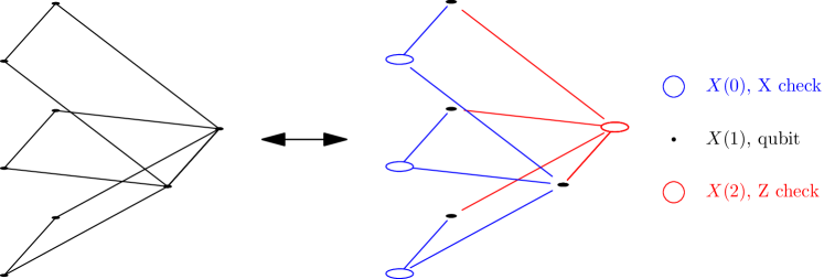
Figure 4: An example of the square complex $\mathcal{G}$ and the balanced product code $X$.

Therefore, to obtain an embedding of the code in $\mathbb{Z}^{D}$, it suffices to obtain an embedding of the square complex in $\mathbb{Z}^{D}$. Unfortunately, $\mathcal{G}$ is an expander and expanders cannot be embedded locally in $\mathbb{Z}^{D}$. Nevertheless, the subdivided square complex $\mathcal{G}_{L}$ introduced later has a local embedding which is how we embed the subdivided code $X_{L}$ in $\mathbb{Z}^{D}$. This will be discussed later in Section 2.5.

2.4 Expansion Properties of Chain Complexes

In the previous subsection, we claimed that the quantum code $Q(X)$ has linear distance and linear energy barrier. To discuss these concepts at once, it is helpful to introduce the notion of small-set (co)boundary expansion initially discussed in [22] and further enhanced in [18]. These expansion properties are natural generalizations of the (co)boundary expansion [35], which will also be used later in the paper.

Definition 2.3 (Small-Set (Co)Boundary Expansion).

We say that $X:\mathbb{F}_{2}^{X(0)}\xrightarrow{\delta_{0}}\mathbb{F}_{2}^{X(1)}\xrightarrow{\delta_{1}}\mathbb{F}_{2}^{X(2)}$ is a $(\alpha,\beta,\gamma)$-small-set boundary expander if

$$\forall c_{1}\in\mathbb{F}_{2}^{X(1)},\lvert c_{1}\rvert\leq\alpha|X(1)|:\exists c_{2}\in\mathbb{F}_{2}^{X(2)},\beta\lvert c_{1}+\partial_{2}c_{2}\rvert\leq\lvert\partial_{1}c_{1}\rvert,\gamma\lvert c_{2}\rvert\leq\lvert c_{1}\rvert.$$

Similarly, $X$ is a $(\alpha,\beta,\gamma)$-small-set coboundary expander if

$$\forall c_{1}\in\mathbb{F}_{2}^{X(1)},\lvert c_{1}\rvert\leq\alpha|X(1)|:\exists c_{0}\in\mathbb{F}_{2}^{X(0)},\beta\lvert c_{1}+\delta_{0}c_{0}\rvert\leq\lvert\delta_{1}c_{1}\rvert,\gamma\lvert c_{0}\rvert\leq\lvert c_{1}\rvert.$$

Roughly speaking, $\alpha$ and $\beta$ correspond to distance and energy barrier, respectively. More precisely, if the chain complex $X$ has $(\alpha,\beta,\gamma)$-small-set boundary and coboundary expansion, then the corresponding quantum code $Q(X)$ has distance $>\alpha|X(1)|=\alpha n$ and energy barrier $\geq\alpha\beta|X(1)|=\alpha\beta n$.

Here is a sketch of the bound on energy barrier.

Proof of energy barrier from small-set coboundary expansion.

Recall the energy barrier is the minimal number of violated checks needed to go from $0$ to a nonzero codeword. Let $\lVert c_{1}\rVert$ be the minimal weight among the vectors in the same homology as $c_{1}$, $\lVert c_{1}\rVert=\min_{c_{0}\in\mathbb{F}_{2}^{X(0)}}|c_{1}+\delta_{0}c_{0}|$. Since a nonzero codeword has weight $\lVert c_{1}\rVert>\alpha|X(1)|$, along the path from $0$ to a nonzero codeword, there has to be a vector of weight $\lVert c_{1}^{\prime}\rVert=\alpha|X(1)|$. Let $c_{1}^{\prime\prime}$ to be the vector of minimal weight in the same homology as $c_{1}^{\prime}$. Since they are in the same homology, they have the same number of violated checks, $|\delta_{1}c_{1}^{\prime\prime}|=|\delta_{1}c_{1}^{\prime}|$. And because $|c_{1}^{\prime\prime}|=\lVert c_{1}^{\prime}\rVert=\alpha|X(1)|$, small-set coboundary expansion applies and we have $\beta|c_{1}^{\prime\prime}|\leq|\delta_{1}c_{1}^{\prime\prime}|$. Therefore, the energy barrier is at least $\alpha\beta|X(1)|$, since we have identified a vector $c_{1}^{\prime}$ on the path with a large number of violated checks $|\delta_{1}c_{1}^{\prime}|=|\delta_{1}c_{1}^{\prime\prime}|\geq\beta|c_{1}^{\prime\prime}|=\alpha\beta|X(1)|$. ∎

Therefore, Theorem 2.2 about distance and energy barrier for $Q(X)$ can be obtained as a corollary of the following theorem, the way it was done in [18].

Theorem 2.4.

$X$ provides a family of bounded degree 3-term chain complexes with $(\alpha,\beta,\gamma)$-small-set boundary expansion and coboundary expansion for certain constants $\alpha,\beta,\gamma$.

Here, bounded degree means LDPC, i.e. $\delta_{0}$ and $\delta_{1}$ have bounded number of nonzero entries in each column and row.

In the special case when $\alpha=1$, $|c_{1}|\leq\alpha|X(1)|=|X(1)|$ imposes no constraints on $c_{1}$ and this is known as the boundary expansion.

Definition 2.5 ((Co)Boundary Expansion).

We say that $X:\mathbb{F}_{2}^{X(0)}\xrightarrow{\delta_{0}}\mathbb{F}_{2}^{X(1)}\xrightarrow{\delta_{1}}\mathbb{F}_{2}^{X(2)}$ is a $\beta$-boundary expander if

$$\forall c_{1}\in\mathbb{F}_{2}^{X(1)}:\exists c_{2}\in\mathbb{F}_{2}^{X(2)},\beta\lvert c_{1}+\partial_{2}c_{2}\rvert\leq\lvert\partial_{1}c_{1}\rvert.$$

Similarly, $X$ is a $\beta$-coboundary expander if

$$\forall c_{1}\in\mathbb{F}_{2}^{X(1)}:\exists c_{0}\in\mathbb{F}_{2}^{X(0)},\beta\lvert c_{1}+\delta_{0}c_{0}\rvert\leq\lvert\delta_{1}c_{1}\rvert.$$

Note that when $X$ is a boundary expander $X$ has to be exact. Suppose $c_{1}\in Z_{1}=\operatorname{ker}\partial_{1}$, i.e. $\partial_{1}c_{1}=0$, the inequality $0=\lvert\partial_{1}c_{1}\rvert\geq\beta\lvert c_{1}+\partial_{2}c_{2}\rvert$ implies $c_{1}+\partial_{2}c_{2}=0$, i.e. $c_{1}=\partial_{2}c_{2}\in B_{1}$. This means $B_{1}=Z_{1}$, i.e. exact.

To fit our proof method, we will later extend the definition of coboundary expansion in Definition 5.1.

2.5 Subdivision of a Square Complex and its Random Embedding in $\mathbb{Z}^{D}$

The overall strategy to construct our geometrically local codes is by composing two maps, one from the code to the square complex, $I_{\textnormal{code}\to\textnormal{square}}$, the other from the square complex to the Euclidean space $\mathbb{Z}^{D}$, $I_{\textnormal{square}\to\textnormal{euclid}}$. We discussed aspects of $I_{\textnormal{code}\to\textnormal{square}}$ in Section 2.3. This section focuses on $I_{\textnormal{square}\to\textnormal{euclid}}$. The strategy of the embedding follows from [8, 6].

Because the square complex is an expander graph which does not have a geometrically local embedding, we have to subdivide it which then has a local embedding.

Definition 2.6 (Subdivide a Square Complex).

Given a square complex $\mathcal{G}=(V,E,F)$, the $L$-subdivision $\mathcal{G}_{L}=(V_{L},E_{L},F_{L})$ is the square complex where each face is subdivided into $L\times L$ squares and the edges and vertices are included accordingly.

Two examples are illustrated in Figure 5.

Figure 5: The subdivision of square complexes.

For the ease of the subdivided code discussed later in Section 3, we assign a coordinate to each vertex in $\mathcal{G}_{L}$. Each vertex has a coordinate $(i,j)$ for some $0\leq i,j\leq L$, depending on its location in the square. Recall that because $\mathcal{G}$ is the balanced product of two bipartite graphs, the vertices of $\mathcal{G}$ can be split into 4 groups, $V(\mathcal{G})=V_{00}\cup V_{10}\cup V_{01}\cup V_{11}$. We assign the coordinate of the vertices in $V_{00},V_{10},V_{01},V_{11}$ as $(0,0),(L,0),(0,L),(L,L)$, respectively. Other vertices in $\mathcal{G}_{L}$ belong to some face $(v_{00},v_{10},v_{01},v_{11})\in F$ and have a corresponding coordinate $(i,j)$.

It is known that for large enough $L$, the subdivided complex $\mathcal{G}_{L}$ has a local embedding with bounded density.

Theorem 2.7 (Modified [6, Theorem 7]).

Given a bounded degree square complex $\mathcal{G}$, the $L$-subdivision $\mathcal{G}_{L}$ has an embedding $f:V(\mathcal{G}_{L})\to\mathbb{Z}^{D}$ with constant $a,b=\Theta(1)$ such that

1. Geometrically local: For all adjacent vertices on the complex $(v_{0},v_{1})\in E(\mathcal{G}_{L})$, the distance of corresponding points in $\mathbb{Z}^{D}$ is bounded $|f(v_{0})-f(v_{1})|\leq a$.

2. Bounded density: The number of vertices at each point is bounded, i.e. for all $x\in\mathbb{Z}^{D}$, $|f^{-1}(x)|\leq b$.

for $L=|V(\mathcal{G})|^{\frac{1}{D-2}}\log^{D+1}|V(\mathcal{G})|$.

We denote this embedding $f$ as $I_{\textnormal{square}_{L}\to\textnormal{euclid}}$ which will be used to embed the subdivided code into $\mathbb{Z}^{D}$.

We summarize the construction and the proof of the theorem. The embedding is obtained by mapping the vertices in $V(\mathcal{G})$ randomly to the sphere of dimension $D-1$ with radius $L^{\prime}=V^{\frac{1}{D-2}}$ where $V=|V(\mathcal{G})|$ is the number of vertices. We then interpolate the points to obtain an embedding for the subdivided square complex with subdivision $L^{\prime}$. The image is currently in $\mathbb{R}^{D}$, so we nudge the vertices slightly so that the image becomes $\mathbb{Z}^{D}$. (We actually need an extra perturbation of the points which will be discussed shortly. This is where the factor $\log^{D+1}V$ appears in $L$.)

The construction automatically satisfies locality, so it suffices to check that the embedding has bounded density. The idea is to take the union bound over the bad events where some unit ball contains too many vertices. The expected number of vertices in a ball is roughly the volume of the square complex with thickness $1$ divided by the volume of the ball of radius $L^{\prime}$. The volume of the square complex is $\Theta({L^{\prime}}^{2}V)$ and the volume of the ball of radius $L^{\prime}$ is $\Theta({L^{\prime}}^{D})$. Therefore, with the choice $L^{\prime}=V^{\frac{1}{D-2}}$, the expected number of vertices in a ball is constant. Using Chernoff bound, the probability that the ball has $\Omega(\log V)$ vertices is then small enough to apply the union bound. However, $\Omega(\log V)$ is not bounded density, so we have to do an extra perturbation and this is why the polylog factor appears in $L$. The full detail can be found in [6, App 1].

2.6 Surface Codes

The surface code [10, 37], also known as the toric code, is a CSS code which is geometrically local and has a planar layout, making it highly suitable for practical quantum computing. In our context, the surface code is the simplest example of the subdivided code that we will define later. Furthermore, many properties of the subdivided code boils down to the properties of the surface code (or more precisely, the generalized surface code), so we give a brief review of the surface code.

Given a subdivided square of size $L\times L$, we can arrange the qubits and the checks based on whether the coordinate $(i,j)$ is even or odd as illustrated in Figure 6. It is known that the surface code has parameters $[[n=(\frac{L}{2}+1)^{2}+(\frac{L}{2})^{2},k=1,d=\frac{L}{2}+1]]$.

However, knowing the distance of the surface code is not enough for the proof we will present later. What we will need is the coboundary expansion properties similar to those defined in Section 2.4. Furthermore, we will have to work with codes that are more general than the surface codes which we call the generalized surface codes. Roughly speaking, these are codes with 2d structures, just like the surface codes, but with extra branching points, similar to the square complexes. The generalized surface codes and their expansion properties will be discussed in Section 5.

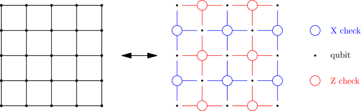
Figure 6: Surface code of size $L=4$.

3 Construct Geometrically Local Codes through Subdivision

Equipped with the knowledge that the balanced product code $X$ has a square complex structure $\mathcal{G}$ as discussed in Section 2.3, we now use this structure to construct the subdivided code $X_{L}$ which has a natural embedding $I_{\textnormal{code}_{L}\to\textnormal{square}_{L}}:\operatorname{Set}(X_{L})\to V(\mathcal{G}_{L})$. After composing with the map $I_{\textnormal{square}_{L}\to\textnormal{euclid}}$ in Section 2.5, this gives the desired local embedding of the subdivided code $I_{\textnormal{code}_{L}\to\textnormal{euclid}}:\operatorname{Set}(X_{L})\to\mathbb{Z}^{D}$.

Take an odd number $L$. We split the vertices of $V(\mathcal{G}_{L})$ into three groups $X_{L}(0),X_{L}(1),X_{L}(2)$ which will be the basis for $X_{L}$. Recall that each vertex in $V(\mathcal{G}_{L})$ has a corresponding coordinate $(i,j)$. We now define

• $X_{L}(0)$ to be the set of vertices with $i,j$ both being even.

• $X_{L}(1)$ to be the set of vertices with $i,j$ one being even, one being odd.

• $X_{L}(2)$ to be the set of vertices with $i,j$ both being odd.

The linear maps are defined by the adjacency matrices, where $X_{L}(0)\xrightarrow{\delta_{0}}X_{L}(1)$ is the adjacency matrix between $X_{L}(0)$ and $X_{L}(1)$ and $X_{L}(1)\xrightarrow{\delta_{1}}X_{L}(2)$ is the adjacency matrix between $X_{L}(1)$ and $X_{L}(2)$. One can check that this defines a chain complex. Two examples are illustrated in Figures 7 and 8.

Remark 3.1.

In the main text, we describe the construction as a subdivision process. An alternative way to understand the construction is through welding [5]. Welding is a process that glues multiple surface codes into a larger code. Our construction is essentially multiple copies of the surface codes on the faces of the balanced product graph welded along the edges. The extra ingredient compared to [5] is that our welding is built on top of the good qLDPC codes which have better code properties.

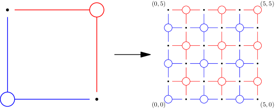
Figure 7: The subdivision of a balanced product code.

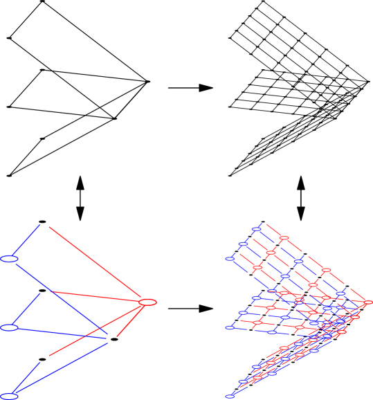
Figure 8: The subdivision of a balanced product code together with the subdivision of the associated square complex.

3.1 Full Construction of the Geometrically Local Quantum Codes

We now have all the ingredients needed to describe the full construction of the geometrically local codes. Recall from Section 2.2 that to describe a geometrically local code in $D$ dimension, we need to specify the parity-check matrices of the code together with an embedding of the qubits and the checks in $\mathbb{Z}^{D}$.

We first describe the parity-check matrices. Let $X$ be the chain complex from [1, 34, 38, 18] that has small-set boundary and coboundary expansion. Let $X_{L}$ be the chain complex after $L$-subdivision defined in the previous subsection. We will set the value of $L$ in a moment. The quantum code $Q(X_{L})$ is defined to have parity-check matrices $H_{z}=\delta_{0}^{T}$ and $H_{x}=\delta_{1}$.

For the embedding, with the appropriate choice of $L=|V(\mathcal{G})|^{\frac{1}{D-2}}\log^{D+1}|V(\mathcal{G})|$ from Theorem 2.7, we have the embedding map $I_{\textnormal{square}_{L}\to\textnormal{euclid}}:V(\mathcal{G}_{L})\to\mathbb{Z}^{D}$ that is geometrically local and has bounded density. Here, $\mathcal{G}$ is the square complex associated to $X$ and $\mathcal{G}_{L}$ is the subdivided square complex. By composing the isomorphism $I_{\textnormal{code}_{L}\to\textnormal{square}_{L}}:\operatorname{Set}(X_{L})\xrightarrow{\sim}V(\mathcal{G}_{L})$ and $I_{\textnormal{square}_{L}\to\textnormal{euclid}}$ we have the embedding

$$I_{\textnormal{code}_{L}\to\textnormal{euclid}}=I_{\textnormal{square}_{L}\to\textnormal{euclid}}\,\circ\,I_{\textnormal{code}_{L}\to\textnormal{square}_{L}}:\operatorname{Set}(X_{L})\to\mathbb{Z}^{D}.$$ (11)

The embedding $I_{\textnormal{code}_{L}\to\textnormal{euclid}}$ induces the embedding of the codes simply because $\operatorname{Set}(Q(X_{L}))=\operatorname{Set}(X_{L})$. This completes the full construction of the geometrically local codes.

We discuss some technical aspect of the code. In our discussion, we will represent the max degree of the bipartite graphs used for the balanced product as $\Delta_{\max}$ and the min degree as $\Delta_{\min}$. (These bipartite graphs $G_{1},G_{2}$ are discussed in Section 2.3.2.) For the sake of making the parameters look simpler, we will use the fact that $\Delta_{\min}\geq 2$, which can be chosen for all the good qLDPC codes above.

3.2 Subcomplexes of the Subdivided Code

The analysis of the subdivided code generally contains two parts. One is about the original code which has been worked out in earlier works. The other is about the subcomplexes that will be discussed in this subsection.

Consider the connected components of $\mathcal{G}_{L}$ when removing all edges of the form $\{(i,L-1),(i,L)\}$ and $\{(L-1,j),(L,j)\}$. We observe that each component contains exactly one of the corner vertices. Additionally, these corner vertices correspond to the vertices in $\mathcal{G}$. This induces a bijection between the vertices in $\mathcal{G}$ and the connected components in $\mathcal{G}_{L}$.

To be formal, we split the vertices $V(\mathcal{G}_{L})$ into 3 groups $S,T,U$ where

• $S$ contains vertices with coordinates $0\leq i,j\leq L-1$.

• $T$ contains vertices with coordinates $i=L,0\leq j\leq L-1$ or $0\leq i\leq L-1,j=L$.

• $U$ contains vertices with coordinates $i=j=L$.

We see that $S,T,U$ are not fully connected and let $\mathcal{S},\mathcal{T},\mathcal{U}$ be the set of connected components of $S,T,U$ respectively. Since each connected components contains exactly one of the corner vertices, we have the bijections $X(0)\cong\mathcal{S}$, $X(1)\cong\mathcal{T}$, $X(2)\cong\mathcal{U}$. See Figure 9.

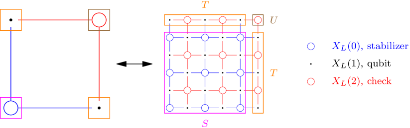
Figure 9: Regions $S$, $T$, $U$ and the bijections $X(0)\cong\mathcal{S}$, $X(1)\cong\mathcal{T}$, $X(2)\cong\mathcal{U}$.

Notice that each component forms a chain complex. Let $S_{i}\in\mathcal{S}$ be one of the components. Then the restriction $X_{L}|_{S_{i}}:\mathbb{F}_{2}^{S_{i}\cap X_{L}(0)}\to\mathbb{F}_{2}^{S_{i}\cap X_{L}(1)}\to\mathbb{F}_{2}^{S_{i}\cap X_{L}(2)}$ is a chain complex. (See Figure 9.) One can similarly study the linear map (technically also a chain complex) $X_{L}|_{T_{i}}:\mathbb{F}_{2}^{T_{i}\cap X_{L}(1)}\to\mathbb{F}_{2}^{T_{i}\cap X_{L}(2)}$ for $T_{i}\in\mathcal{T}$. (Note that $T_{i}\cap X_{L}(0)=0$ and $X_{L}|_{U_{i}}$ is just a vertex.) These chain complexes (subcomplexes) will be essential for the analysis of the subdivided code. Since $X_{L}|_{S_{i}}$ and $X_{L}|_{T_{i}}$ share similarities to the surface code and the repetition code, we call them the generalized surface code and the generalized repetition code which are depicted in Figure 10.

We discuss a few features of these subcomplexes. More of their properties will be studied in Section 5. Notice that the generalized surface code has a product structure. It is the tensor product of two generalized repetition codes. This property comes from the fact that the balanced product code is locally a product. The generalized repetition code is like a tree with a unique branching point. Notice that the number of branches corresponds to the degree of some vertex in the bipartite graphs $G_{1},G_{2}$. As reminder, this number is between $\Delta_{\min}=2$ and $\Delta_{\max}=\Theta(1)$.

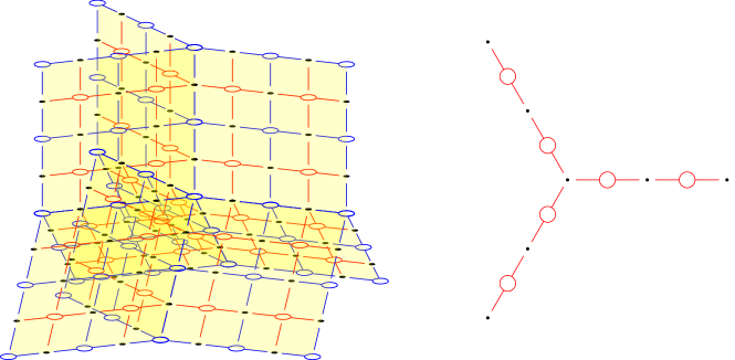
Figure 10: Generalized surface code and generalized repetition code.

We now define the chain maps $\mathcal{F}_{i}:\mathbb{F}_{2}^{X(i)}\to\mathbb{F}_{2}^{X_{L}(i)}$ for $i=0,1,2$ that will be used repeatedly in the analysis later.

• Given $\widetilde{c}_{0}\in\mathbb{F}_{2}^{X(0)}$, we define $\mathcal{F}_{0}(\widetilde{c}_{0})\in\mathbb{F}_{2}^{X_{L}(0)}$ by repeating the value $\widetilde{c}_{0}(v)$ at the corresponding component $S_{i}$ of $v$ for each $v\in X(0)$.

• Given $\widetilde{c}_{1}\subset\mathbb{F}_{2}^{X(1)}$, we define $\mathcal{F}_{1}(\widetilde{c}_{1})\in\mathbb{F}_{2}^{X_{L}(1)}$ by repeating the value $\widetilde{c}_{1}(v)$ at the corresponding component $T_{i}$ of $v$ for each $v\in X(1)$ and set other values in $S$ to be $0$.

• Given $\widetilde{c}_{2}\subset\mathbb{F}_{2}^{X(2)}$, we define $\mathcal{F}_{2}(\widetilde{c}_{2})\in\mathbb{F}_{2}^{X_{L}(2)}$ by setting the value $\widetilde{c}_{2}(v)$ at the corresponding vertex $U_{i}$ of $v$ for each $v\in X(2)$ and set other values in $S$ and $T$ to be $0$.

Notice that these maps commutes with $\delta$. In particular,

(12)

Many of the later proofs will be moving back and forth between the two chain complexes through $\mathcal{F}$. Notice that $\mathcal{F}_{i}$ are injective because by construction they are repeating values.

Applying the discussions above, we can show the following bounds on $X_{L}(i)$.

Claim 3.2.

$$L^{2}|X(i)|\leq|X_{L}(i)|\leq\frac{\Delta_{\max}^{2}}{4}L^{2}|X(i)|$$ (13)

for all $i=0,1,2$. In particular, $|X_{L}(i)|=\Theta(L^{2}|X(i)|)$.

Proof.

We show the case for $i=0$. Other cases follow similarly by noticing the symmetry that $\mathcal{G}$ is a 4-partite graph and $X(0),X(1),X(2)$ contain $1,2,1$ parts, respectively.

To proof utilize the isomorphism $X(0)\cong\mathcal{S}$. Notice that each connected component $S_{i}\in\mathcal{S}$ contains $(\Delta_{1}\frac{L-1}{2}+1)(\Delta_{2}\frac{L-1}{2}+1)$ vertices in $X_{L}(0)$ where $\Delta_{1}$ and $\Delta_{2}$ are the degrees of branchings. (One way to see this is that $S_{i}$ has a product structure and the each piece contains $\Delta_{j}\frac{L-1}{2}+1$ vertices.) Since $2\leq\Delta_{1},\Delta_{2}\leq\Delta_{\max}$, the number of vertices in each component is between $L^{2}$ and $(\Delta_{\max}\frac{L-1}{2}+1)^{2}\leq\frac{\Delta_{\max}^{2}}{4}L^{2}$. Hence, we have the result. ∎

It is helpful to express the size of various sets in terms of $L$. Let $V=|V(\mathcal{G})|=|X(0)|+|X(1)|+|X(2)|$. Recall $L=V^{\frac{1}{D-2}}\operatorname{polylog}V$, i.e. $V=L^{D-2}/\operatorname{polylog}L$. It is known that $|X(0)|,|X(1)|,|X(2)|=\Theta(V)=\Theta(L^{D-2}/\operatorname{polylog}L)$. Combining with the claim above, we have

$$|X(0)|,|X(1)|,|X(2)| =\Theta(L^{D-2}/\operatorname{polylog}L),$$ (14)

$$|X_{L}(0)|,|X_{L}(1)|,|X_{L}(2)| =\Theta(L^{D}/\operatorname{polylog}L).$$ (15)

4 Properties of the Subdivided Code

Having constructed the codes in the previous section, we now study their properties and show Theorem 1.1. We will use the common names stabilizers, qubits, checks to refer to elements in $X_{L}(0),X_{L}(1),X_{L}(2)$, respectively.

We will adopt the following notations. $c_{1}|_{S}$ denotes the restriction of the vector $c_{1}$ to the support on $S$ (equivalently $S\cap X_{L}(1)$). $|c_{1}|_{S}$ denotes the Hamming weight of the restricted vector $c_{1}|_{S}$.

4.1 Geometric Locality and Bounded Density

We first show that the codes have the desired geometric properties.

Lemma 4.1.

The codes $Q(X_{L})$ are geometrically local and have bounded density.

Proof.

Notice that $\operatorname{Set}(X_{L})=V(\mathcal{G}_{L})$ and the qubit-check relations of the code are precisely the adjacency relations of $\mathcal{G}_{L}$. This implies that it suffices to check $I_{\textnormal{square}_{L}\to\textnormal{euclid}}:V(\mathcal{G}_{L})\to\mathbb{Z}^{D}$ is geometrically local and has bounded density. This holds because of Theorem 2.7. ∎

4.2 Dimension

We next show that the codes retain the same dimensions. Essentially, what we want to show is that $\mathcal{F}:X\to X_{L}$ induces a quasi-isomorphism, i.e. $Z^{i}(X)/B^{i}(X)\xrightarrow{\sim}Z^{i}(X_{L})/B^{i}(X_{L})$ are isomorphisms for all $i$. Intuitively, this holds for the same reason that cellular homology of a manifold is independent of the choice of the cellulation. However, we will not go through those discussions. We will show $Z^{i}(X)/B^{i}(X)\xrightarrow{\sim}Z^{i}(X_{L})/B^{i}(X_{L})$ for $i=1$ directly by brute force.

Lemma 4.2.

If the code $Q(X)$ has dimension $k$ then the code $Q(X_{L})$ has dimension $k$.

Proof.

The goal is to show that $\mathcal{F}_{1}$ induces a bijection between the codewords (equivalent classes) $Z^{1}(X)/B^{1}(X)$ and $Z^{1}(X_{L})/B^{1}(X_{L})$ by mapping $[\widetilde{c}_{1}]$ to $[\mathcal{F}_{1}(\widetilde{c}_{1})]$. To show this, we need to show

1. $\widetilde{c}_{1}\in B^{1}(X)\implies\mathcal{F}_{1}(\widetilde{c}_{1})\in B^{1}(X_{L})$.

2. $\widetilde{c}_{1}\in Z^{1}(X)\implies\mathcal{F}_{1}(\widetilde{c}_{1})\in Z^{1}(X_{L})$.

3. $\mathcal{F}_{1}(\widetilde{c}_{1})\in B^{1}(X_{L})\implies\widetilde{c}_{1}\in B^{1}(X)$.

4. Given $c_{1}\in Z^{1}(X_{L})$, there exists $\widetilde{c}_{1}\in Z^{1}(X)$, such that $c_{1}\in[\mathcal{F}_{1}(\widetilde{c}_{1})]$.

The first two imply that the map $[\widetilde{c}_{1}]\mapsto[\mathcal{F}_{1}(\widetilde{c}_{1})]$ is well-defined and maps $Z^{1}(X)/B^{1}(X)$ to $Z^{1}(X_{L})/B^{1}(X_{L})$. The last two imply that the map is injective and surjective, respectively. So, overall, we get a bijection. We show the desired statements one by one.

1. $\widetilde{c}_{1}\in B^{1}(X)\implies\mathcal{F}_{1}(\widetilde{c}_{1})\in B^{1}(X_{L})$.

Because $\widetilde{c}_{1}\in B^{1}(X)$ there exists $\widetilde{c}_{0}\in\mathbb{F}_{2}^{X(0)}$ such that $\widetilde{c}_{1}=\delta_{1}\widetilde{c}_{0}$. The statement then follows from the left block of the commutative diagram in Equation 12, $\mathcal{F}_{1}(\widetilde{c}_{1})=\mathcal{F}_{1}(\delta_{0}\widetilde{c}_{0})=\delta_{0}\mathcal{F}_{0}(\widetilde{c}_{0})$.

2. $\widetilde{c}_{1}\in Z^{1}(X)\implies\mathcal{F}_{1}(\widetilde{c}_{1})\in Z^{1}(X_{L})$.

This follows from the right block of the commutative diagram in Equation 12, $\delta_{1}\mathcal{F}_{1}(\widetilde{c}_{1})=\mathcal{F}_{2}(\delta_{1}\widetilde{c}_{1})=0$.

3. $\mathcal{F}_{1}(\widetilde{c}_{1})\in B^{1}(X_{L})\implies\widetilde{c}_{1}\in B^{1}(X)$.

Let $c_{1}=\mathcal{F}_{1}(\widetilde{c}_{1})$ and let $c_{0}\in\mathbb{F}_{2}^{X_{L}(0)}$ be the vector that satisfies $\delta_{0}c_{0}=c_{1}$. Since $c_{1}|_{S}=0$, $c_{0}$ takes the same value in each connected component $S_{i}\in\mathcal{S}$. That means $c_{0}\in\operatorname{im}\mathcal{F}_{0}$.

Let $\widetilde{c}_{0}=\mathcal{F}_{0}^{-1}(c_{0})$. We claim that $\delta_{0}c_{0}=\widetilde{c}_{1}$. From the left block of the commutative diagram in Equation 12, we have $\mathcal{F}_{1}(\delta_{0}\widetilde{c}_{0})=\delta_{0}\mathcal{F}_{0}(\widetilde{c}_{0})=\delta_{0}c_{0}=c_{1}=\mathcal{F}_{1}(\widetilde{c}_{1})$. Since $\mathcal{F}_{1}$ is injective $\delta_{0}c_{0}=\widetilde{c}_{1}$.

4. Given $c_{1}\in Z^{1}(X_{L})$, there exists $\widetilde{c}_{1}\in Z^{1}(X)$, such that $c_{1}\in[\mathcal{F}_{1}(\widetilde{c}_{1})]$.

We first construct $c_{1}^{\prime}\in\operatorname{im}\mathcal{F}_{1}$ by removing the support of $c_{1}$ in $S$. Notice that the chain complex $X_{L}|_{S}:\mathbb{F}_{2}^{S\cap X_{L}(0)}\to\mathbb{F}_{2}^{S\cap X_{L}(1)}\to\mathbb{F}_{2}^{S\cap X_{L}(2)}$ is exact because the subcomplex $X_{L}|_{S_{i}}$ is exact for each connected component $S_{i}\in\mathcal{S}$. Since $\delta_{1}c_{1}=0$, $c_{1}|_{S}\in Z^{1}(X_{L}|_{S})=B^{1}(X_{L}|_{S})$. Therefore, there exists $c_{0}\in\mathbb{F}_{2}^{S\cap X_{L}(0)}=\mathbb{F}_{2}^{X_{L}(0)}$ such that $(c_{1}+\delta_{0}c_{0})|_{S}=0$. So $c_{1}^{\prime}=c_{1}+\delta_{0}c_{0}$ is not supported in $S$ and is only supported in $T$.

To show $c_{1}^{\prime}\in\operatorname{im}\mathcal{F}_{1}$, we additionally need to show that $c_{1}^{\prime}$ takes the same value in each connected component $T_{i}\in\mathcal{T}$. Notice that $c_{1}^{\prime}\in Z^{1}(X_{L})$ which means $c_{1}^{\prime}$ violates no checks. Each check in $T_{i}$ acts on two qubits in $T_{i}$ and some other qubits in $S$. Since $c_{1}^{\prime}$ is not supported in $S$, the two nearby qubits in $T_{i}$ take the same value. Hence, $c_{1}^{\prime}$ take the same value in each connected component.

Let $\widetilde{c}_{1}=\mathcal{F}_{1}^{-1}(c_{1}^{\prime})$. We suffice to show $\widetilde{c}_{1}\in Z^{1}(X)$. From the right block of the commutative diagram in Equation 12, $\mathcal{F}_{2}(\delta_{1}\widetilde{c}_{1})=\delta_{1}\mathcal{F}_{1}(\widetilde{c}_{1})=\delta_{1}c_{1}^{\prime}=0$. Since $\mathcal{F}_{2}$ is injective $\delta_{1}\widetilde{c}_{1}=0$ which concludes the proof. ∎

Corollary 4.3.

$Q(X_{L})$ has dimensions $\Omega(n^{\frac{D-2}{D}}/\operatorname{polylog}n)$.

Proof.

We first prove the case of $Q(X_{L})$ where $n=|X_{L}(1)|$. Recall that Equations 14 and 15 say $|X(1)|=\Theta(L^{D-2}/\operatorname{polylog}L)$ and $|X_{L}(1)|=\Theta(L^{D}/\operatorname{polylog}L)$. Thus, $k(X_{L})=k(X)=\Theta(|X(1)|)=\Theta(L^{D-2}/\operatorname{polylog}L)=\Omega(n^{\frac{D-2}{D}}/\operatorname{polylog}n)$, where the second equality follows from the fact that good codes have linear dimension. ∎

4.3 Distance, Energy Barrier: By Showing Small-Set Boundary Expansion

We now show the rest of the code properties. As discussed in Section 2.4, we will show them by showing the subdivided code has boundary and coboundary expansion. As a reminder we say a chain complex has $(\alpha,\beta,\gamma)$-coboundary expansion if

$$\forall c_{1}\in\mathbb{F}_{2}^{X(1)},\lvert c_{1}\rvert\leq\alpha|X(1)|:\exists c_{0}\in\mathbb{F}_{2}^{X(0)},\beta\lvert c_{1}+\delta_{0}c_{0}\rvert\leq\lvert\delta_{1}c_{1}\rvert,\gamma\lvert c_{0}\rvert\leq\lvert c_{1}\rvert.$$

Theorem 4.4.

If $X$ has $(\alpha_{\textnormal{qLDPC}},\beta_{\textnormal{qLDPC}},\gamma_{\textnormal{qLDPC}})$-small-set coboundary (boundary) expansion, then $X_{L}$ has $(\alpha,\beta,\gamma)$-small-set coboundary (boundary) expansion where

$$\alpha=\frac{\eta_{0}^{\textnormal{sur}}}{4L}\frac{4}{\Delta_{\max}^{2}}\alpha_{\textnormal{qLDPC}},\quad\beta=\frac{1}{\frac{1}{\beta_{1}^{\textnormal{sur}}}+\frac{1}{\beta^{\textnormal{rep}}\eta_{1}^{\textnormal{sur}}}+\frac{1}{\beta_{\textnormal{qLDPC}}\eta^{\textnormal{rep}}\eta_{1}^{\textnormal{sur}}}\frac{\Delta_{\max}}{2}L},\quad\gamma=\frac{1}{\frac{2}{\beta_{0}^{\textnormal{sur}}}+\frac{4}{\gamma_{\textnormal{qLDPC}}\eta_{0}^{\textnormal{sur}}}\frac{\Delta_{\max}^{2}}{4}L}.$$ (16)

In our context $\beta_{0}^{\textnormal{sur}},\beta_{1}^{\textnormal{sur}},\beta^{\textnormal{rep}}=\Theta(1/L)$ and $\eta_{0}^{\textnormal{sur}},\eta_{1}^{\textnormal{sur}},\eta^{\textnormal{rep}},\alpha_{\textnormal{qLDPC}},\beta_{\textnormal{qLDPC}},\gamma_{\textnormal{qLDPC}},\Delta_{\max}=\Theta(1)$. Thus, $\alpha,\beta,\gamma=\Theta(1/L)$.

With that we have the following results.

Corollary 4.5.

$Q(X_{L})$ has distance $\Omega(n^{\frac{D-1}{D}}/\operatorname{polylog}(n))$ and energy barrier $\Omega(n^{\frac{D-2}{D}}/\operatorname{polylog}(n))$.

Proof.

Let $n=|X_{L}(1)|$. As discussed in Section 2.4, distance $d\geq\alpha|X_{L}(1)|$ and energy barrier $\mathcal{E}\geq\alpha\beta|X_{L}(1)|$. Recall that Equation 15 say $|X_{L}(1)|=\Theta(L^{D}/\operatorname{polylog}L)$. Thus, $d(X_{L})=\Omega(\alpha|X_{L}(1)|)=\Theta(L^{D-1}/\operatorname{polylog}L)=\Omega(n^{\frac{D-1}{D}}/\operatorname{polylog}n)$ and $\mathcal{E}(X_{L})=\Omega(\alpha\beta|X_{L}(1)|)=\Theta(L^{D-2}/\operatorname{polylog}L)=\Omega(n^{\frac{D-2}{D}}/\operatorname{polylog}n)$. ∎

Before proving the full theorem, we prove the following simpler theorem as a warm up.

Theorem 4.6 (A simplification of Theorem 4.4).

If $X$ has cosystolic (systolic) distance $\alpha_{\textnormal{qLDPC}}$, then $X_{L}$ has cosystolic (systolic) distance $\alpha=\frac{\eta_{0}^{\textnormal{sur}}}{2L}\frac{4}{\Delta_{\max}^{2}}\alpha_{\textnormal{qLDPC}}$. More explicitly,

$$\forall c_{1}\in Z^{1}(X_{L}),|c_{1}|\leq\alpha|X_{L}(1)|:c_{1}\in B^{1}(X_{L}).$$ (17)

This means that if $Q(X)$ has linear distance, then $Q(X_{L})$ has distance $\Theta(n/L)$ where $n=|X_{L}(1)|$ is the number of qubits.

In the following, we only study the coboundary and cosystolic properties. Notice that $X$ and $X_{L}$ are symmetric when flipping the direction of the chain complexes. So the argument that applies to the coboundary expansion also applies to the boundary expansion. Therefore, it suffices to study the coboundary expansion.

The proof will utilize the coboundary expansion properties of the generalized surface codes and the generalized repetition codes in Section 5. We have stated the consequences of coboundary expansion properties explicitly in the proof, so it is not required to have a full understanding of Section 5 before reading the proof below. For reference, the definitions and the lemma statements that is used in the proof can be found in Section 5.2.

Proof.

We first outline the proof. To show $c_{1}\in B^{1}(X_{L})$, the idea is to first reduce the question to another codeword $c_{1}^{\prime}$ in the same homology, i.e. $c_{1}-c_{1}^{\prime}\in B^{1}(X_{L})$. (Here, being a codeword means being a systole, i.e. $c_{1}^{\prime}\in Z^{1}(X_{L})$.) If we can show $c_{1}^{\prime}\in B^{1}(X_{L})$, this implies $c_{1}\in B^{1}(X_{L})$.

The codeword $c_{1}^{\prime}$ will be constructed in a way so that it is supported in specific 1d-like regions and has a small weight. This is achieved using the expansion properties of the generalized surface code.

Because of the structure of $c_{1}^{\prime}$’s support, $c_{1}^{\prime}$ can then be associated with another codeword $\widetilde{c}_{1}$ in the old code $X$, which again has a small weight.

Now, we invoke the distance assumption that small weight codewords of $X$ are boundaries. That means $\widetilde{c}_{1}\in B^{1}(X)$ which, in turn, implies $c_{1}^{\prime}\in B^{1}(X_{L})$, and thus $c_{1}\in B^{1}(X_{L})$.

We now go through each step in detail.

Step 1: Construct $c_{1}^{\prime}$ by removing $c_{1}$ in $S$, i.e. 2d cleaning.

Notice that each connected region of $S$ is a generalized surface code, which has expansion properties by Corollary 5.5. The same applies to their disjoint union with the same expansion parameters. By applying Corollary 5.5 to the disjoint regions of $S$ with $\hat{f}_{1}=c_{1}$, there exist $c^{S}_{0}=f_{0}$ and $c^{S}_{1}=f_{1}$ supported on $S$ which satisfy

$$(a)\,c_{1}|_{S}=(\delta_{0}c^{S}_{0}+c^{S}_{1})|_{S},\quad(b)\,\frac{\beta^{\textnormal{sur}}_{0}}{2}|c^{S}_{0}|_{S}\leq|c_{1}|_{S},\quad(c)\,\beta^{\textnormal{sur}}_{1}|c^{S}_{1}|_{S}\leq|\delta_{1}c_{1}|_{S},\quad\\ (d)\,\frac{\eta^{\textnormal{sur}}_{0}}{2}|\delta_{0}c^{S}_{0}|_{T}\leq|c_{1}|_{S},\quad(e)\,\eta^{\textnormal{sur}}_{1}|\delta_{1}c^{S}_{1}|_{T}\leq|\delta_{1}c_{1}|_{S}.$$ (18)

(The superscript in $c^{S}_{0}$ is a reminder that its support is in $S$. The subscript is a reminder that $c^{S}_{0}$ is a $0$-chain, i.e. $c^{S}_{0}\in\mathbb{F}_{2}^{X_{L}(0)}$.) Notice $c^{S}_{1}|_{S}=0$, because (c) $\beta_{1}^{\textnormal{sur}}|c^{S}_{1}|_{S}\leq|\delta_{1}\hat{c}^{S}_{1}|_{S}=0$. We then define $c_{1}^{\prime}=c_{1}+\delta_{0}c^{S}_{0}$. Notice $c_{1}^{\prime}$ has no support in $S$ because (a) $c_{1}^{\prime}|_{S}=(c_{1}+\delta_{0}c^{S}_{0})|_{S}=c^{S}_{1}|_{S}=0$.

Additionally, we have control of the weight $|c_{1}^{\prime}|$:

$$|c_{1}^{\prime}| =|c_{1}^{\prime}|_{T}$$

$$\leq|c_{1}|_{T}+|\delta_{0}c^{S}_{0}|_{T}$$

$$\leq|c_{1}|_{T}+\frac{2}{\eta^{\textnormal{sur}}_{0}}|c_{1}|_{S}$$

$$\leq\frac{2}{\eta^{\textnormal{sur}}_{0}}|c_{1}|$$ (19)

where the third inequality uses (d) and the last inequality uses $1\leq\frac{2}{\eta^{\textnormal{sur}}_{0}}$.

Step 2: Construct $c_{1}^{\prime\prime}$ by making $c_{1}^{\prime}$ consistent in $T$, i.e. 1d cleaning.

We say $c_{1}^{\prime}$ is consistent on $T$, if for each connected region $T_{i}\subset T$, $c_{1}^{\prime}$ takes the same value on $T_{i}$. In the current simpler context, $c_{1}^{\prime}$ is already consistent, because $c_{1}^{\prime}\in Z^{1}$, i.e. $\delta_{1}c_{1}^{\prime}=0$, which means $c_{1}^{\prime}$ does not violate any check. Notice that the check in $T_{i}$ acts on two qubits in $T_{i}$ and some other qubits in $S$. Given that $c_{1}^{\prime}$ is not supported in $S$, the two qubits in $T_{i}$ must take the same value. Therefore, within the connected region $T_{i}$, all qubits take the same value.

Step 3: Construct $\widetilde{c}_{1}$ from $c_{1}^{\prime\prime}$ by moving from $X_{L}$ to $X$.

The consistency of $c_{1}^{\prime}$ and the fact that $c_{1}^{\prime}$ is not supported in $S$ implies $c_{1}^{\prime}\in\operatorname{im}\mathcal{F}_{1}$. We define $\widetilde{c}_{1}=\mathcal{F}_{1}^{-1}(c_{1}^{\prime})$.

Notice that the small weight of $c_{1}^{\prime}$ implies the small weight of $\widetilde{c}_{1}$. Because each region $T_{i}$ has size at least $|T_{i}\cap X_{L}(1)|\geq L$, each nonzero value is repeated at least $L$ times. This implies $|\widetilde{c}_{1}|\leq|c_{1}^{\prime}|/L$.

Step 4: Construct $\widetilde{c}_{0}$ from $\widetilde{c}_{1}$ by applying expansion assumption of $X$.

Combine the above, we obtain that the weight $|\widetilde{c}_{1}|$ is small:

$$|\widetilde{c}_{1}|\leq|c_{1}^{\prime}|/L\leq\frac{2}{\eta^{\textnormal{sur}}_{0}L}|c_{1}|\leq\frac{2}{\eta^{\textnormal{sur}}_{0}L}\alpha|X_{L}(1)|\leq\frac{2L}{\eta^{\textnormal{sur}}_{0}}\frac{\Delta_{\max}^{2}}{4}\alpha|X(1)|=\alpha_{\textnormal{qLDPC}}|X(1)|$$

where the second inequality uses Equation 19 and the fourth inequality uses 3.2, $|X_{L}(1)|\leq\frac{\Delta_{\max}^{2}}{4}L^{2}|X(1)|$. Therefore, we can apply the expansion assumption and obtain $\widetilde{c}_{1}\in B^{1}(X)$, i.e. there exist $\widetilde{c}_{0}\in\mathbb{F}_{2}^{X(0)}$ such that $\widetilde{c}_{1}=\delta_{0}\widetilde{c}_{0}$.

Step 5 and wrap up.

To complete the proof, we need to show $c_{1}^{\prime}\in B^{1}(X_{L})$. This is done by lifting $\widetilde{c}_{0}\in\mathbb{F}_{2}^{X(0)}$ into $c_{0}=\mathcal{F}_{0}(\widetilde{c}_{0})\in\mathbb{F}_{2}^{X_{L}(0)}$. We have $c_{1}^{\prime}=\mathcal{F}_{1}(\widetilde{c}_{1})=\mathcal{F}_{1}(\delta_{0}\widetilde{c}_{0})=\delta_{0}\mathcal{F}_{0}(\widetilde{c}_{0})=\delta_{0}c_{0}$, where the third equality uses the left block of the commutative diagram Equation 12. ∎

With the proof of the simpler theorem in mind, we are ready to use the same template to show Theorem 4.4.

Proof of Theorem 4.4.

Recall that because $X$ and $X_{L}$ are symmetric, it suffices to study the coboundary expansion which we will now focus on.

Step 1: Construct $c_{1}^{\prime}$ by removing $c_{1}$ in $S$, i.e. 2d cleaning.

By applying Corollary 5.5 to the disjoint regions of $S$ with $\hat{f}_{1}=c_{1}$, there exist $c^{S}_{0}=f_{0}$ and $c^{S}_{1}=f_{1}$ supported on $S$ which satisfy

$$(a)\,c_{1}|_{S}=(\delta_{0}c^{S}_{0}+c^{S}_{1})|_{S},\quad(b)\,\frac{\beta^{\textnormal{sur}}_{0}}{2}|c^{S}_{0}|_{S}\leq|c_{1}|_{S},\quad(c)\,\beta^{\textnormal{sur}}_{1}|c^{S}_{1}|_{S}\leq|\delta_{1}c_{1}|_{S},\quad\\ (d)\,\frac{\eta^{\textnormal{sur}}_{0}}{2}|\delta_{0}c^{S}_{0}|_{T}\leq|c_{1}|_{S},\quad(e)\,\eta^{\textnormal{sur}}_{1}|\delta_{1}c^{S}_{1}|_{T}\leq|\delta_{1}c_{1}|_{S}.$$ (20)

We then set $c_{1}^{\prime}$ to be $c_{1}+\delta_{0}c^{S}_{0}$ restricted to the support on $T\cup U$. Notice that $T\cup U$ is the complement of $S$. So by (a),

$$c_{1}+\delta_{0}c^{S}_{0}=c^{S}_{1}+c_{1}^{\prime}.$$ (21)

Intuitively, $c^{S}_{0}$ tries to clean up $c_{1}$ in $S$ using the coboundaries $\delta_{0}c^{S}_{0}$ as much as possible and $c^{S}_{1}$ removes the remaining support in $S$. The rest of the vector supported in $T\cup U$ is $c_{1}^{\prime}$.

The inequalities (b) and (c) bound the resource needed to remove the support of $c_{1}$ in $S$, which is intuitively saying that one can control the difference between $c_{1}^{\prime}$ and $c_{1}$. On the other hand, the inequalities (d) and (e) bound the unwanted effect created in $T\cup U$ caused by the cleaning process, which is intuitively saying that $c_{1}^{\prime}$ has small weight. More concretely, we have the following bounds on the weight

$$|c_{1}^{\prime}| =|c_{1}^{\prime}|_{T}$$

$$\leq|\delta_{0}c^{S}_{0}|_{T}+|c_{1}|_{T}$$

$$\leq\frac{2}{\eta_{0}^{\textnormal{sur}}}|c_{1}|_{S}+|c_{1}|_{T}$$

$$\leq\frac{2}{\eta_{0}^{\textnormal{sur}}}|c_{1}|$$ (22)

where the third inequality uses (d) and the last inequality uses $1\leq\frac{2}{\eta_{0}^{\textnormal{sur}}}$. Furthermore,

$$|\delta_{1}c_{1}^{\prime}| =|\delta_{1}c_{1}^{\prime}|_{T}+|\delta_{1}c_{1}^{\prime}|_{U}$$

$$\leq|\delta_{1}c^{S}_{1}|_{T}+|\delta_{1}c_{1}|_{T}+|\delta_{1}c_{1}|_{U}$$

$$\leq\frac{1}{\eta_{1}^{\textnormal{sur}}}|\delta_{1}c_{1}|_{S}+|\delta_{1}c_{1}|_{T}+|\delta_{1}c_{1}|_{U}$$

$$\leq\frac{1}{\eta_{1}^{\textnormal{sur}}}|\delta_{1}c_{1}|$$ (23)

where the second inequality uses $|\delta_{1}c_{1}^{\prime}|_{U}=|\delta_{1}c_{1}|_{U}$ because by Equation 21, $\delta_{1}c_{1}^{\prime}-\delta_{1}c_{1}=\delta_{1}c^{S}_{1}$ which is supported only in $T$. The third inequality uses (e) and the last inequality uses $1\leq\frac{1}{\eta_{1}^{\textnormal{sur}}}$.

Step 2: Construct $c_{1}^{\prime\prime}$ by making $c_{1}^{\prime}$ consistent in $T$, i.e. 1d cleaning.

By applying Corollary 5.4 to the disjoint regions of $T$ with $\hat{f}_{0}=c_{1}^{\prime}$, there exists $c^{T}_{1}=f_{0}$ supported on $T$ which satisfies

$$(a)\,c_{1}^{\prime}+c^{T}_{1}\in B^{1},\quad(b)\,|c^{T}_{1}|_{T}\leq|c_{1}^{\prime}|_{T},\quad(c)\,\beta^{\textnormal{rep}}|c^{T}_{1}|_{T}\leq|\delta_{1}c_{1}^{\prime}|_{T},\quad(d)\,\eta^{\textnormal{rep}}|\delta_{1}c^{T}_{1}|_{U}\leq|\delta_{1}c_{1}^{\prime}|_{T}.$$ (24)

We then set $c_{1}^{\prime\prime}$ to be $c_{1}^{\prime}+c^{T}_{1}$ which by (a) violates no checks in $T$, i.e. consistent in $T$.

We can again bound the weight properties of $c_{1}^{\prime\prime}$

$$|c_{1}^{\prime\prime}|=|c_{1}^{\prime}+c^{T}_{1}|_{T}\leq|c_{1}^{\prime}|_{T}+|c^{T}_{1}|_{T}\leq 2|c_{1}^{\prime}|_{T}\leq\frac{4}{\eta_{0}^{\textnormal{sur}}}|c_{1}|$$ (25)

where the third inequality uses (b) and the last inequality uses Equation 22. Further,

$$|\delta_{1}c_{1}^{\prime\prime}| =|\delta_{1}c_{1}^{\prime\prime}|_{U}$$

$$\leq|\delta_{1}c^{T}_{1}|_{U}+|\delta_{1}c_{1}^{\prime}|_{U}$$

$$\leq\frac{1}{\eta^{\textnormal{rep}}}|\delta_{1}c_{1}^{\prime}|_{T}+|\delta_{1}c_{1}^{\prime}|_{U}$$

$$\leq\frac{1}{\eta^{\textnormal{rep}}}|\delta_{1}c_{1}^{\prime}|$$

$$\leq\frac{1}{\eta^{\textnormal{rep}}\eta_{1}^{\textnormal{sur}}}|\delta_{1}c_{1}|$$ (26)

where the third inequality uses (d) and the last inequality uses Equation 23.

Step 3: Construct $\widetilde{c}_{1}$ from $c_{1}^{\prime\prime}$ by moving from $X_{L}$ to $X$.

Because $c_{1}^{\prime\prime}$ is consistent on each connected region of $T$, we can define $\widetilde{c}_{1}=\mathcal{F}_{1}^{-1}(c_{1}^{\prime\prime})\in\mathbb{F}_{2}^{X(1)}$ as in the proof of Theorem 4.6.

Because each connected region of $T$ has size $\geq L$, we can again bound the weight properties of $\widetilde{c}_{1}$ where $|\widetilde{c}_{1}|\leq|c_{1}^{\prime\prime}|/L$. Furthermore, $|\delta_{1}\widetilde{c}_{1}|=|\delta_{1}c_{1}^{\prime\prime}|$ because all the checks in $T$ are satisfied and by the construction of $\mathcal{F}_{1}$, $|\delta_{1}\widetilde{c}_{1}|_{U}=|\delta_{1}c_{1}^{\prime\prime}|_{U}$. (Another way to see this is to use the commutative diagram Equation 12 $\delta_{1}c_{1}^{\prime\prime}=\delta_{1}\mathcal{F}_{1}(c_{1})=\mathcal{F}_{2}(\delta_{1}\widetilde{c}_{1})$. Notice that $\mathcal{F}_{2}$ does not change the weight of the vector by construction. Hence, $|\delta_{1}\widetilde{c}_{1}|=|\delta_{1}c_{1}^{\prime\prime}|$.)

Step 4: Construct $\widetilde{c}_{0}$ from $\widetilde{c}_{1}$ by applying expansion assumption of $X$.

Notice the weight $\widetilde{c}_{1}$ is small:

$$|\widetilde{c}_{1}|\leq|c_{1}^{\prime\prime}|/L\leq\frac{4}{\eta_{0}^{\textnormal{sur}}L}|c_{1}|\leq\frac{4}{\eta_{0}^{\textnormal{sur}}L}\alpha|X_{L}(1)|\leq\frac{4L}{\eta_{0}^{\textnormal{sur}}}\frac{\Delta_{\max}^{2}}{4}\alpha|X(1)|=\alpha_{\textnormal{qLDPC}}|X(1)|$$

where the fourth inequality uses 3.2, $|X_{L}(1)|\leq\frac{\Delta_{\max}^{2}}{4}L^{2}|X(1)|$. Therefore, by the expansion assumption of $X$, there exist $\widetilde{c}_{0}\in X(0)$ such that $\beta_{\textnormal{qLDPC}}|\widetilde{c}_{1}+\delta_{0}\widetilde{c}_{0}|\leq|\delta_{1}\widetilde{c}_{1}|$ and $\gamma_{\textnormal{qLDPC}}|\widetilde{c}_{0}|\leq|\widetilde{c}_{1}|$.

Step 5: Construct $c_{0}^{\prime\prime}$ from $\widetilde{c}_{0}$ by moving back from $X$ to $X_{L}$.

Same as in the proof of Theorem 4.6, we lift $\widetilde{c}_{0}$ to $c_{0}^{\prime\prime}=\mathcal{F}_{0}(\widetilde{c}_{0})\in\mathbb{F}_{2}^{X_{L}(0)}$.

Notice that each entry of $\widetilde{c}_{0}$ is repeated $\leq(\Delta_{\max}\frac{L-1}{2}+1)^{2}\leq\frac{\Delta_{\max}^{2}}{4}L^{2}$ times, and each entries of $\widetilde{c}_{1}$ is repeated between $L$ and $\Delta_{\max}\frac{L-1}{2}+1\leq\frac{\Delta_{\max}}{2}L$ times. Therefore, $\beta_{\textnormal{qLDPC}}|\widetilde{c}_{1}+\delta_{0}\widetilde{c}_{0}|\leq|\delta_{1}\widetilde{c}_{1}|$ lifts into

$$\beta_{\textnormal{qLDPC}}|c_{1}^{\prime\prime}+\delta_{0}c_{0}^{\prime\prime}|\leq\frac{\Delta_{\max}}{2}L|\delta_{1}c_{1}^{\prime\prime}|$$ (27)

because $|c_{1}^{\prime\prime}+\delta_{0}c_{0}^{\prime\prime}|\leq\frac{\Delta_{\max}}{2}L|\widetilde{c}_{1}+\delta_{0}\widetilde{c}_{0}|$ and $|\delta_{1}\widetilde{c}_{1}|=|\delta_{1}c_{1}^{\prime\prime}|$. Further, $\gamma_{\textnormal{qLDPC}}|\widetilde{c}_{0}|\leq|\widetilde{c}_{1}|$ lifts into

$$\gamma_{\textnormal{qLDPC}}|c_{0}^{\prime\prime}|\leq\frac{\Delta_{\max}^{2}}{4}L|c_{1}^{\prime\prime}|$$ (28)

because $|c_{0}^{\prime\prime}|\leq\frac{\Delta_{\max}^{2}}{4}L^{2}|\widetilde{c}_{0}|$ and $L|\widetilde{c}_{1}|\leq|c_{1}^{\prime\prime}|$.

Wrap up.

We are ready to construct $c_{0}$ with the desired bound $\beta|c_{1}+\delta_{0}c_{0}|\leq|\delta_{1}c_{1}|$ and $\gamma|c_{0}|\leq|c_{1}|$. This is done by utilizing the vectors we have derived from $c_{1}$ in the process above, $c_{0}^{S},c_{1}^{S},c_{1}^{\prime},c_{1}^{T},c_{1}^{\prime\prime},\widetilde{c}_{1},\widetilde{c}_{0},c_{0}^{\prime\prime}$, and their associated inequalities.

We set $c_{0}=c_{0}^{S}+c_{0}^{\prime\prime}$ and check the inequalities:

$$|c_{1}+\delta_{0}c_{0}| =|c_{1}+\delta_{0}c_{0}^{S}+\delta_{0}c_{0}^{\prime\prime}|$$

$$=|c_{1}^{S}+c_{1}^{\prime}+\delta_{0}c_{0}^{\prime\prime}|$$

$$=|c_{1}^{S}+c_{1}^{T}+c_{1}^{\prime\prime}+\delta_{0}c_{0}^{\prime\prime}|$$

$$\leq|c_{1}^{S}|+|c_{1}^{T}|+|c_{1}^{\prime\prime}+\delta_{0}c_{0}^{\prime\prime}|$$

$$\leq\frac{1}{\beta_{1}^{\textnormal{sur}}}|\delta_{1}c_{1}|+\frac{1}{\beta^{\textnormal{rep}}}|\delta_{1}c_{1}^{\prime}|_{T}+\frac{1}{\beta_{\textnormal{qLDPC}}}\frac{\Delta_{\max}}{2}L|\delta_{1}c_{1}^{\prime\prime}|$$

$$\leq\frac{1}{\beta_{1}^{\textnormal{sur}}}|\delta_{1}c_{1}|+\frac{1}{\beta^{\textnormal{rep}}\eta_{1}^{\textnormal{sur}}}|\delta_{1}c_{1}|+\frac{1}{\beta_{\textnormal{qLDPC}}\eta^{\textnormal{rep}}\eta_{1}^{\textnormal{sur}}}\frac{\Delta_{\max}}{2}L|\delta_{1}c_{1}|$$

$$=\left(\frac{1}{\beta_{1}^{\textnormal{sur}}}+\frac{1}{\beta^{\textnormal{rep}}\eta_{1}^{\textnormal{sur}}}+\frac{1}{\beta_{\textnormal{qLDPC}}\eta^{\textnormal{rep}}\eta_{1}^{\textnormal{sur}}}\frac{\Delta_{\max}}{2}L\right)|\delta_{1}c_{1}|$$ (29)

where the second and third equality holds by construction. The fifth inequality uses Equation 20(c), Equation 24(c) and Equation 27. The sixth inequality uses Equations 23 and 26. Finally,

$$|c_{0}| =|c_{0}^{S}+c_{0}^{\prime\prime}|$$

$$\leq|c_{0}^{S}|+|c_{0}^{\prime\prime}|$$

$$\leq\frac{2}{\beta_{0}^{\textnormal{sur}}}|c_{1}|_{S}+\frac{1}{\gamma_{\textnormal{qLDPC}}}\frac{\Delta_{\max}^{2}}{4}L|c_{1}^{\prime\prime}|$$

$$\leq\frac{2}{\beta_{0}^{\textnormal{sur}}}|c_{1}|+\frac{4}{\gamma_{\textnormal{qLDPC}}\eta_{0}^{\textnormal{sur}}}\frac{\Delta_{\max}^{2}}{4}L|c_{1}|$$

$$=\left(\frac{2}{\beta_{0}^{\textnormal{sur}}}+\frac{4}{\gamma_{\textnormal{qLDPC}}\eta_{0}^{\textnormal{sur}}}\frac{\Delta_{\max}^{2}}{4}L\right)|c_{1}|$$ (30)

where the third inequality uses Equation 20(b) and Equation 28. The fourth inequality uses Equation 25. This completes the proof. ∎

5 Properties of the Generalized Repetition Code and the Generalized Surface Code

This section focuses on the two Corollaries 5.4 and 5.5 that are used in the proof of Theorem 4.4 in the previous section. They are derived from Lemmas 5.2 and 5.3 which are about the coboundary expansion properties of the generalized repetition code and the generalized surface code.

We briefly recall how Corollaries 5.4 and 5.5 were used in the proof of Theorem 4.4. The proof of Theorem 4.4 is to reduce the question of the expansion property of the subdivided code $X_{L}$ to the expansion property of the original code $X$. This reduction is achieved by cleaning up the vector $c_{1}$ into $c_{1}^{\prime}$ then into $c_{1}^{\prime\prime}$. This cleaning is where Corollaries 5.4 and 5.5 comes in. The property used in cleaning is coboundary expansion and an additional condition that tracks some property on the “boundary”.

We will discuss this additional condition later in more detail. For now, we just want to mention that when defining the generalized repetition code and the generalized surface code, we additionally consider their “boundary”. In particular, the chain complex $\mathbb{F}_{2}^{Y(i)}\xrightarrow{\delta_{i}}\mathbb{F}_{2}^{Y(i+1)}\xrightarrow{\delta_{i+1}}\mathbb{F}_{2}^{Y(i+2)}$ is extended to have the additional structure $\mathbb{F}_{2}^{Y(i)\cup Y_{\partial}(i)}\xrightarrow{\delta_{i}^{\prime}}\mathbb{F}_{2}^{Y(i+1)\cup Y_{\partial}(i+1)}\xrightarrow{\delta_{i+1}^{\prime}}\mathbb{F}_{2}^{Y(i+2)\cup Y_{\partial}(i+2)}$. We will refer to this structure as a chain complex with boundary. To simplify the notation, from now on $\delta_{i}:\mathbb{F}_{2}^{Y(i)\cup Y_{\partial}(i)}\to\mathbb{F}_{2}^{Y(i+1)\cup Y_{\partial}(i+1)}$ will mean the map that includes the boundary. We will use $|f_{i}|_{\textnormal{int}}$ to denote the Hamming weight of the vector in $Y$, i.e. $|f_{i}|_{\textnormal{int}}=|\operatorname{supp}f_{i}\cap Y(i)|$ (the subscript stands for interior), and use $|f_{i}|_{\partial}$ to denote the Hamming weight in $Y_{\partial}$, i.e. $|f_{i}|_{\partial}=|\operatorname{supp}f_{i}\cap Y_{\partial}(i)|$.

5.1 The Generalized Repetition Code and the Generalized Surface Code

We first define the generalized repetition code and the generalized surface code, then describe their expansion properties.

The repetition code is a 1d chain of bits connected by a 1d chain of checks which require the neighboring bits to be the same. The generalized repetition code is similar, except that now there could be one branching point at the center. See Figure 11. The adjacency matrix defines the map $\mathbb{F}_{2}^{Y(0)}\to\mathbb{F}_{2}^{Y(1)\cup Y_{\partial}(1)}$. This can be extended to $Y^{\textnormal{rep}}:\mathbb{F}_{2}\xrightarrow{\delta_{-1}}\mathbb{F}_{2}^{Y(0)}\xrightarrow{\delta_{0}}\mathbb{F}_{2}^{Y(1)\cup Y_{\partial}(1)}$ where $\delta_{-1}$ maps $1$ to the all $1$ vector. Notice that the restriction of the linear maps to the interior, $\mathbb{F}_{2}\xrightarrow{\delta_{-1}|_{Y}}\mathbb{F}_{2}^{Y(0)}\xrightarrow{\delta_{0}|_{Y}}\mathbb{F}_{2}^{Y(1)}$, is a chain complex.

We say a generalized repetition code has length $L$ if there are $L$ bits on the path from one boundary to another boundary. Although the definition of length may seem arbitrary, it is defined in a way that eliminates the need for additional conversions when applying the result to the previous section.

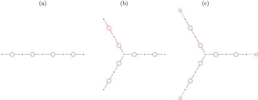
Figure 11: The figure illustrates the generalized repetition codes of length $5$. The black dots are the bits $X(0)$ and the red circles are the checks $X(1)$. (a) The standard repetition code. (b) The generalized repetition code with degree $3$ branching at the center. (c) The same generalized repetition code with boundaries illustrated using the smaller circles.

The surface code is the tensor product of two repetition codes. Similarly, the generalized repetition code is the tensor product of two generalized repetition codes. See Figure 12. The adjacency matrices define the map $\mathbb{F}_{2}^{Y(0)}\to\mathbb{F}_{2}^{Y(1)\cup Y_{\partial}(1)}\to\mathbb{F}_{2}^{Y(2)\cup Y_{\partial}(2)}$ which again can be extended to $Y^{\textnormal{sur}}:\mathbb{F}_{2}\xrightarrow{\delta_{-1}}\mathbb{F}_{2}^{Y(0)}\xrightarrow{\delta_{0}}\mathbb{F}_{2}^{Y(1)\cup Y_{\partial}(1)}\xrightarrow{\delta_{1}}\mathbb{F}_{2}^{Y(2)\cup Y_{\partial}(2)}$ where $\delta_{-1}$ maps $1$ to the all $1$ vector. Notice that the restriction of the linear maps on the interior, $\mathbb{F}_{2}\xrightarrow{\delta_{-1}|_{Y}}\mathbb{F}_{2}^{Y(0)}\xrightarrow{\delta_{0}|_{Y}}\mathbb{F}_{2}^{Y(1)}\xrightarrow{\delta_{1}|_{Y}}\mathbb{F}_{2}^{Y(2)}$, is a chain complex. We say a generalized surface code has length $L$ if the two generalized repetition codes have length $L$.

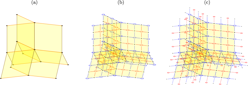
Figure 12: The figure illustrates the generalized surface codes of length $5$. The blue circles are the stabilizers $X(0)$, the black dots are the qubits $X(1)$, and the red circles are the checks $X(2)$. (a) The scaffold is the Cartesian product of two Y-shaped structure with degree $3$ branching. (b) The generalized surface code. (c) The same generalized surface code with boundaries illustrated using the smaller circles.

5.2 Expansion Properties of the Generalized Repetition Code and the Generalized Surface Code

Having defined the generalized repetition code and generalized surface code, we now describe the desired expansion properties.

Definition 5.1.

A chain complex $Y$ with boundary $Y_{\partial}$ is a $(\beta_{i},\eta_{i})$-coboundary expander at level $i$ if for all $\hat{f}_{i}\in\mathbb{F}_{2}^{Y(i)}$, there exists $f_{i}\in\hat{f}_{i}+B^{i}\subset\mathbb{F}_{2}^{Y(i)}$ (recall $B^{i}=\operatorname{im}\delta_{i-1}|_{Y}$ where both the domain and the range are restricted to $Y$.) such that

$$(1)\,|f_{i}|_{\textnormal{int}}\leq|\hat{f}_{i}|_{\textnormal{int}},\quad(2)\,\beta_{i}|f_{i}|_{\textnormal{int}}\leq|\delta_{i}\hat{f}_{i}|_{\textnormal{int}},\quad(3)\,\eta_{i}|\delta_{i}f_{i}|_{\partial}\leq|\delta_{i}\hat{f}_{i}|_{\textnormal{int}}.$$ (31)

Inequality (2) is the standard coboundary expansion for $Y$ in Definition 2.5 and inequality (3) is the extra inequality which bounds the newly introduced objects during cleaning.

The following two lemmas say the generalized repetition code and the generalized surface code have coboundary expansion property. We will use the subscript to keep track of the level we are discussing.

Lemma 5.2.

A generalized repetition code with size $L$, $Y^{\textnormal{rep}}$, is a $(\beta_{0}=\frac{2}{L},\eta_{0}=1)$-coboundary expander at level $0$.

Lemma 5.3.

A generalized surface code with size $L$, $Y^{\textnormal{sur}}$, is a $(\beta_{0}=\frac{1}{L},\eta_{0}=\frac{L-1}{4L})$-coboundary expander at level $0$ and a $(\beta_{1}=\frac{2}{3L},\eta_{1}=\frac{1}{2})$-coboundary expander at level $1$.

We attempt to phrase the lemmas above to elucidate the structure. However, it is not obvious how the current statements relate to the main proof presented in the previous section. So the following rephrasing seeks to enhance explicitness and usability.

Corollary 5.4.

Given a generalized repetition code with size $L$, $Y^{\textnormal{rep}}:\mathbb{F}_{2}\xrightarrow{\delta_{-1}}\mathbb{F}_{2}^{Y(0)}\xrightarrow{\delta_{0}}\mathbb{F}_{2}^{Y(1)\cup Y_{\partial}(1)}$, for all $\hat{f}_{0}\in\mathbb{F}_{2}^{Y(0)}$, there exists $f_{0}\in\mathbb{F}_{2}^{Y(0)}$ such that

$$(a)\,\hat{f}_{0}+f_{0}\in B^{0},\quad(b)\,|f_{0}|_{\textnormal{int}}\leq|\hat{f}_{0}|_{\textnormal{int}},\quad(c)\,\beta^{\textnormal{rep}}|f_{0}|_{\textnormal{int}}\leq|\delta_{0}\hat{f}_{0}|_{\textnormal{int}},\quad(d)\,\eta^{\textnormal{rep}}|\delta_{0}f_{0}|_{\partial}\leq|\delta_{0}\hat{f}_{0}|_{\textnormal{int}},$$ (32)

with $\beta^{\textnormal{rep}}=\frac{2}{L}$ and $\eta^{\textnormal{rep}}=1$.

Proof of Corollary 5.4.

By Lemma 5.2, we can find $f_{0}\in\hat{f}_{0}+B^{0}$ where $f_{0}$ satisfies the inequalities in Equation 31 at level $i=0$. By construction, we have (a). One easily check that (1) $\implies$ (b), (2) $\implies$ (c), (3) $\implies$ (d). ∎

Corollary 5.5.

Given a generalized surface code with size $L$, $Y^{\textnormal{sur}}:\mathbb{F}_{2}\xrightarrow{\delta_{-1}}\mathbb{F}_{2}^{Y(0)}\xrightarrow{\delta_{0}}\mathbb{F}_{2}^{Y(1)\cup Y_{\partial}(1)}\xrightarrow{\delta_{1}}\mathbb{F}_{2}^{Y(2)\cup Y_{\partial}(2)}$, for all $\hat{f}_{1}\in\mathbb{F}_{2}^{Y(1)}$, there exist $f_{0}\in\mathbb{F}_{2}^{Y(0)}$ and $f_{1}\in\mathbb{F}_{2}^{Y(1)}$ such that

$$(a)\,\hat{f}_{1}=(\delta_{0}f_{0}+f_{1})|_{\textnormal{int}},\quad(b)\,\frac{\beta^{\textnormal{sur}}_{0}}{2}|f_{0}|_{\textnormal{int}}\leq|\hat{f}_{1}|_{\textnormal{int}},\quad(c)\,\beta^{\textnormal{sur}}_{1}|f_{1}|_{\textnormal{int}}\leq|\delta_{1}\hat{f}_{1}|_{\textnormal{int}},\quad\\ (d)\,\frac{\eta^{\textnormal{sur}}_{0}}{2}|\delta_{0}f_{0}|_{\partial}\leq|\hat{f}_{1}|_{\textnormal{int}},\quad(e)\,\eta^{\textnormal{sur}}_{1}|\delta_{1}f_{1}|_{\partial}\leq|\delta_{1}\hat{f}_{1}|_{\textnormal{int}},$$ (33)

with $\beta^{\textnormal{sur}}_{0}=\frac{1}{L},\eta^{\textnormal{sur}}_{0}=\frac{L-1}{4L},\beta^{\textnormal{sur}}_{1}=\frac{2}{3L},\eta^{\textnormal{sur}}_{0}=\frac{1}{2}$.

Proof of Corollary 5.5.

By Lemma 5.3, we can write $\hat{f}_{1}=f_{1}+(\delta_{0}\hat{f}_{0})|_{\textnormal{int}}$ for some $\hat{f}_{0}\in\mathbb{F}_{2}^{X(0)}$ where $f_{1}$ satisfies the inequalities in Equation 31 at level $i=1$. And we can find $f_{0}\in\hat{f}_{0}+B^{0}$ where $f_{0}$ satisfies the inequalities in Equation 31 at level $i=0$. By construction, we have (a). One can check that (2) at level 1 $\implies$ (c) and (3) at level 1 $\implies$ (e). To show (b) and (d), we use (2) and (3) at level 0, $\beta^{\textnormal{sur}}_{0}|f_{0}|_{\textnormal{int}}\leq|\delta_{0}\hat{f}_{0}|_{\textnormal{int}}$ and $\eta^{\textnormal{sur}}_{0}|\delta_{0}f_{0}|_{\partial}\leq|\delta_{0}\hat{f}_{0}|_{\textnormal{int}}$ together with

$$|\delta_{0}\hat{f}_{0}|_{\textnormal{int}}\leq|\hat{f}_{1}|_{\textnormal{int}}+|f_{1}|_{\textnormal{int}}\leq 2|\hat{f}_{1}|_{\textnormal{int}}$$ (34)

where the last inequality uses (1) at level 1, $|f_{1}|_{\textnormal{int}}\leq|\hat{f}_{1}|_{\textnormal{int}}$. ∎

The remainder of this section is devoted to showing Lemmas 5.2 and 5.3.

5.3 Proof of Lemma 5.2 for Generalized Repetition Codes

We observe that there are only two elements in $\hat{f}_{0}+B^{0}$ since $B^{0}=\{0,\mathbbm{1}\}$ where $0$ is the all $0$ vector and $\mathbbm{1}$ is the all $1$ vector. So all is left is to figure out which choice satisfies the inequalities. We denote $\Delta$ as the degree of the branching. We call the branching point the root.

Proof of Lemma 5.2.

We set $f_{0}=\hat{f}_{0}$ if $|\hat{f}_{0}|_{\textnormal{int}}\leq|Y(0)|/2$. Otherwise, we set $f_{0}=\hat{f}_{0}+\mathbbm{1}$. This immediately satisfies inequality (1) $|f_{0}|_{\textnormal{int}}\leq|\hat{f}_{0}|_{\textnormal{int}}$. Notice that $|f_{0}|_{\textnormal{int}}\leq|Y(0)|/2$.

We now show (2) $\beta_{0}|f_{0}|_{\textnormal{int}}\leq|\delta_{0}\hat{f}_{0}|_{\textnormal{int}}$ with $\beta_{0}=\frac{2}{L}$. If $|\delta_{0}\hat{f}_{0}|_{\textnormal{int}}\geq\Delta/2$, because $|f_{0}|_{\textnormal{int}}\leq|Y(0)|/2$ and $|Y(0)|=\Delta\frac{L-1}{2}+1$, the inequality is satisfied. Otherwise, $|\delta_{0}\hat{f}_{0}|_{\textnormal{int}}<\Delta/2$, this means $\delta_{0}\hat{f}_{0}|_{\textnormal{int}}$ is not supported on $\Delta-|\delta_{0}\hat{f}_{0}|_{\textnormal{int}}$ branches which means these branches take the same value as the root. We observe that this value has to be $0$ otherwise the root and at least half of the branches have value $1$ which violates $|f_{0}|_{\textnormal{int}}\leq|Y(0)|/2$. Therefore, $|f_{0}|_{\textnormal{int}}\leq\frac{L}{2}|\delta_{0}\hat{f}_{0}|_{\textnormal{int}}$, since $f_{0}$ can be supported on at most $|\delta_{0}\hat{f}_{0}|_{\textnormal{int}}$ branches and each branch has weight at most $\frac{L}{2}$.

Finally, we show (3) $\eta_{0}|\delta_{0}f_{0}|_{\partial}\leq|\delta_{0}\hat{f}_{0}|_{\textnormal{int}}$ with $\eta_{0}=1$. We divide the $\Delta$ branches into different groups based on the number of $1$s of $\delta_{0}\hat{f}_{0}|_{\textnormal{int}}$ in each branch. Let $s,t,u$ be the number of branches with no $1$, with an odd number of $1$s, and an even nonzero number of $1$s, respectively. Then $|\delta_{0}\hat{f}_{0}|_{\textnormal{int}}\geq t+2u$. If the root value of $f_{0}$ is $0$, then $|\delta_{0}f_{0}|_{\partial}=t$ which satisfies the inequality $|\delta_{0}f_{0}|_{\partial}\leq|\delta_{0}\hat{f}_{0}|_{\textnormal{int}}$. Otherwise, the root value of $f_{0}$ is $1$, then $|\delta_{0}f_{0}|_{\partial}=s+u$. So it suffices to show $s\leq t+u$. Notice these $s$ branches takes the same value as the root which is $1$. Since $|f_{0}|_{\textnormal{int}}\leq|Y(0)|/2$, this means $s$ covers at most half of the $\Delta$ branches. Thus, $s\leq t+u$. ∎

5.4 Proof of Lemma 5.3 for Generalized Surface Codes

One might hope to demonstrate the expansion of the generalized surface code using two facts: (1) the generalized surface code is a tensor product of two generalized repetition codes (2) the expansion property is preserved under tensor product. It is indeed the case that we can establish the level $0$ expansion through this approach, which we will explain. However, it is not clear to us if a tensor product argument applies to the level $1$ expansion. Therfore, we will show the level $1$ expansion in an ad hoc method through case studies. It would be appealing to have a simpler proof.

5.4.1 Level $0$ Expansion

Note that the level $0$ expansion is essentially the isoperimetric inequalities which is known to behave nicely under tensor product [39, 40]. This gives inequality (2). To show inequality (3), we will apply a similar proof technique.

Consider the graph $\mathcal{G}_{1}$ corresponding to the generalized repetition code where $Y^{\textnormal{rep}}(0)$ are the vertices and $Y^{\textnormal{rep}}(1)$ (without $Y^{\textnormal{rep}}_{\partial}(1)$) are the edges. Similarly, consider the graph $\mathcal{G}$ corresponding to the generalized surface code where $Y^{\textnormal{sur}}(0)$ are the vertices and $Y^{\textnormal{sur}}(1)$ (without $Y^{\textnormal{sur}}_{\partial}(1)$) are the edges. We observe that the graph from the generalized surface code $\mathcal{G}$ is the Cartesian product of two graphs $\mathcal{G}_{1}$ and $\mathcal{G}_{2}$ originating from the generalized repetition code. To capture the notion of boundary $|\delta_{0}f_{0}|_{\partial}$ in the context of graphs, we also consider the boundary vertices which are the vertices in $Y^{\textnormal{rep}}$ ($Y^{\textnormal{sur}}$) next to $Y^{\textnormal{rep}}_{\partial}$ ($Y^{\textnormal{sur}}_{\partial}$). See Figure 13.

Definition 5.6 (Cartesian product of two graphs with boundary).

Given two (undirected) graphs $\mathcal{G}_{1}$ and $\mathcal{G}_{2}$. Let $V_{i}$, $E_{i}$, and $V_{i}^{\partial}\subset V_{i}$ be the vertex set, the edge set, and the boundary vertex set of $\mathcal{G}_{i}$, respectively.

The Cartesian product of two graphs $\mathcal{G}_{1}$ and $\mathcal{G}_{2}$, denoted as $\mathcal{G}_{1}\times\mathcal{G}_{2}$, is a graph with vertex set $V=V_{1}\times V_{2}$ and two vertices $(x_{1},x_{2})$ and $(y_{1},y_{2})$ are adjacent iff $x_{2}=y_{2}$ and $\{x_{1},y_{1}\}$ is an edge of $\mathcal{G}_{1}$ or $x_{1}=y_{1}$ and $\{x_{2},y_{2}\}$ is an edge of $\mathcal{G}_{2}$ which can be expressed as $E=(E_{1}\times V_{2})\cup(V_{1}\times E_{2})$. The new boundary vertex (multi)set is $V^{\partial}=(V_{1}^{\partial}\times V_{2})\sqcup(V_{1}\times V_{2}^{\partial})$, where $\sqcup$ is the disjoint union.

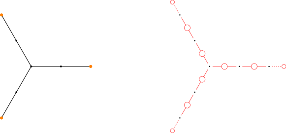
Figure 13: An illustration of $\mathcal{G}_{1}$ on the left that corresponds to $Y^{\textnormal{rep}}$ on the right. Note that $V_{1}^{\partial}$ is marked in orange.

We interpret $V^{\partial}$ as a multiset which double counts the vertices $V_{1}^{\partial}\times V_{2}^{\partial}$ so that $|\delta_{0}f_{0}|_{\partial}$ for the generalized surface code can be expressed as $\sum_{x\in V^{\partial}}1_{f_{0}(x)\neq 0}$.

It is known that isoperimetric inequalities are closely related to functional inequalities. These functional inequalities behave nicely under tensor product. Therefore, our strategy is to use the functional inequalities of the generalized repetition codes to derive the functional inequalities for the generalized surface codes, which will then give the desired isoperimetric inequalities.

Definition 5.7.

We say a graph with boundary $\mathcal{G}=(V,E,V^{\partial})$ satisfies $(C,C^{\partial})$-functional inequalities if for all function $h:V\to\{0,1\}$

$$\sum_{\{x,y\}\in E}|h(x)-h(y)|\geq\frac{C}{|V|}\sum_{x,y\in V}|h(x)-h(y)|,$$ (35)

$$\sum_{\{x,y\}\in E}|h(x)-h(y)|\geq\frac{C^{\partial}}{|V^{\partial}|}\sum_{x\in V^{\partial},y\in V}|h(x)-h(y)|.$$ (36)

Lemma 5.8.

If $\mathcal{G}_{1},\mathcal{G}_{2}$ satisfy $(C,C^{\partial})$-functional inequalities, then $\mathcal{G}_{1}\times\mathcal{G}_{2}$ satisfies $(C,\min(C,C^{\partial}))$-functional inequalities.

We will prove the lemma at the end of this section. We first discuss how the functional inequalities and the coboundary expander are related. We then combine everything to prove the level $0$ coboundary expansion of the surface code.

Let $h$ be $f_{0}$ where $f_{0}$ is the vector with the smaller weight between $\hat{f}_{0}$ and $\hat{f}_{0}+\mathbbm{1}$. In the language of chain complexes, the two functional inequalities become

$$|\delta_{0}f_{0}|_{\textnormal{int}}\geq\frac{C}{|V|}2|f_{0}|\Big{(}|V|-|f_{0}|\Big{)},$$ (37)

$$|\delta_{0}f_{0}|_{\textnormal{int}}\geq\frac{C^{\partial}}{|V^{\partial}|}\bigg{(}|\delta_{0}f_{0}|_{\partial}\Big{(}|V|-|f_{0}|\Big{)}+\Big{(}|V^{\partial}|-|\delta_{0}f_{0}|_{\partial}\Big{)}|f_{0}|\bigg{)}.$$ (38)

Applying this relation, we obtain the following facts.

Claim 5.9.

The graphs corresponding to the generalized repetition code $\mathcal{G}_{1},\mathcal{G}_{2}$ satisfy $(C=\frac{1}{L},C^{\partial}=\frac{1}{L})$-functional inequalities.

Proof.

Recall the generalized repetition code has $(\beta_{0}=\frac{2}{L},\eta_{0}=1)$-coboundary expansion. In particular, for $|f_{0}|\leq|V|/2$

$$|\delta_{0}f_{0}|_{\textnormal{int}}\geq\frac{2}{L}|f_{0}|,$$ (39)

$$|\delta_{0}f_{0}|_{\textnormal{int}}\geq|\delta_{0}f_{0}|_{\partial}.$$ (40)

Since $|V|\geq|V|-|f_{0}|$ and $|V^{\partial}|\geq|V^{\partial}|-|\delta_{0}f_{0}|_{\partial}$, the inequalities above imply

$$|\delta_{0}f_{0}|_{\textnormal{int}}\geq\frac{1/L}{|V|}2|f_{0}||V|\geq\frac{1/L}{|V|}2|f_{0}|\Big{(}|V|-|f_{0}|\Big{)},$$ (41)

$$\Big{(}\frac{L}{2}+\frac{L}{2}\Big{)}|\delta_{0}f_{0}|_{\textnormal{int}} \geq\frac{L}{2}|\delta_{0}f_{0}|_{\partial}+|f_{0}|$$ (42)

$$\geq\frac{1}{|V^{\partial}|}\Big{(}|\delta_{0}f_{0}|_{\partial}|V|+|V^{\partial}||f_{0}|\Big{)}$$ (43)

$$\geq\frac{1}{|V^{\partial}|}\bigg{(}|\delta_{0}f_{0}|_{\partial}\Big{(}|V|-|f_{0}|\Big{)}+\Big{(}|V^{\partial}|-|\delta_{0}f_{0}|_{\partial}\Big{)}|f_{0}|\bigg{)}$$ (44)

where the second inequality uses $\frac{L}{2}\geq\frac{|V|}{|V^{\partial}|}$.

Thus, by comparing to Equations 37 and 38, the functional inequalities are satisfied for $(C=\frac{1}{L},C^{\partial}=\frac{1}{L})$. ∎

Claim 5.10.

If the graph with boundary satisfies $(C,C^{\partial})$-functional inequalities, then the corresponding complex is a $(\beta_{0}=C,\eta_{0}=\frac{C^{\partial}|V|}{2|V^{\partial}|})$-coboundary expander at level $0$.

Proof.

Let $f_{0}$ be the vector with the smaller weight between $\hat{f}_{0}$ and $\hat{f}_{0}+\mathbbm{1}$. Since $|f_{0}|\leq|V|/2$, Equations 37 and 38 imply

$$|\delta_{0}f_{0}|_{\textnormal{int}}\geq C|f_{0}|,$$ (45)

$$|\delta_{0}f_{0}|_{\textnormal{int}}\geq\frac{C^{\partial}|V|}{2|V^{\partial}|}|\delta_{0}f_{0}|_{\partial}.$$ (46)

∎

We now combine the above to prove the level $0$ coboundary expansion of the surface code.

Proof of Lemma 5.3 at level $0$.

By 5.9, $\mathcal{G}_{1},\mathcal{G}_{2}$ satisfy $(C=\frac{1}{L},C^{\partial}=\frac{1}{L})$-functional inequalities. Together with Lemma 5.8, this implies $\mathcal{G}$ satisfies $(\frac{1}{L},\frac{1}{L})$-functional inequalities. Together with 5.10, this implies the generalized surface code satisfies $(\beta_{0}=\frac{1}{L},\eta_{0}=\frac{L-1}{4L})$-coboundary expansion, where we use $\frac{|V|}{|V^{\partial}|}=\frac{|V_{1}||V_{2}|}{|V_{1}^{\partial}||V_{2}|+|V_{1}||V_{2}^{\partial}|}\geq\frac{L-1}{4}$ which holds because $\frac{|V_{1}|}{|V_{1}^{\partial}|},\frac{|V_{2}|}{|V_{2}^{\partial}|}\geq\frac{L-1}{2}$. ∎

We now go back and prove the lemma.

Proof of Lemma 5.8.

We first review the proof of Equation 35 in [40], then extend the proof to Equation 36. The idea is to first split the edges into those running horizontally and those running vertically. We then apply the functional inequalities for $\mathcal{G}_{1}$ and $\mathcal{G}_{2}$. Finally, we use the triangle inequality to rewrite the terms.

$$\sum_{\{x,y\}\in E}|f(x)-f(y)| =\sum_{\{x_{1},y_{1}\}\in E_{1},x_{2}\in V_{2}}|f(x_{1},x_{2})-f(y_{1},x_{2})|+\sum_{y_{1}\in V_{1},\{x_{2},y_{2}\}\in E_{2}}|f(y_{1},x_{2})-f(y_{1},y_{2})|$$

$$\geq\frac{C}{|V_{1}|}\sum_{x_{1},y_{1}\in V_{1},x_{2}\in V_{2}}|f(x_{1},x_{2})-f(y_{1},x_{2})|+\frac{C}{|V_{2}|}\sum_{y_{1}\in V_{1},x_{2},y_{2}\in V_{2}}|f(y_{1},x_{2})-f(y_{1},y_{2})|$$

$$\geq\frac{C}{|V_{1}||V_{2}|}\sum_{x_{1},y_{1}\in V_{1},x_{2},y_{2}\in V_{2}}|f(x_{1},x_{2})-f(y_{1},y_{2})|$$

$$=\frac{C}{|V|}\sum_{x,y\in V}|f(x)-f(y)|$$

We now apply the same technique to Equation 36, but this time, we do it in reverse order.

$$\sum_{x\in V^{\partial},y\in V}|f(x)-f(y)| =\sum_{x\in V_{1}^{\partial}\times V_{2},y\in V}|f(x)-f(y)|+\sum_{x\in V_{1}\times V_{2}^{\partial},y\in V}|f(x)-f(y)|$$

$$\leq|V_{2}|\sum_{x_{1}\in V_{1}^{\partial},y_{1}\in V_{1},x_{2}\in V_{2}}|f(x_{1},x_{2})-f(y_{1},x_{2})|+|V_{1}^{\partial}|\sum_{y_{1}\in V_{1},x_{2},y_{2}\in V_{2}}|f(y_{1},x_{2})-f(y_{1},y_{2})|$$

$$+|V_{1}|\sum_{x_{1}\in V_{1},x_{2}\in V_{2}^{\partial},y_{2}\in V_{2}}|f(x_{1},x_{2})-f(x_{1},y_{2})|+|V_{2}^{\partial}|\sum_{x_{1},y_{1}\in V_{1},y_{2}\in V_{2}}|f(x_{1},y_{2})-f(y_{1},y_{2})|$$

$$\leq\frac{|V_{1}^{\partial}||V_{2}|}{C^{\partial}}\sum_{\{x_{1},y_{1}\}\in E_{1},x_{2}\in V_{2}}|f(x_{1},x_{2})-f(y_{1},x_{2})|+\frac{|V_{1}^{\partial}||V_{2}|}{C}\sum_{y_{1}\in V_{1},\{x_{2},y_{2}\}\in E_{2}}|f(y_{1},x_{2})-f(y_{1},y_{2})|$$

$$+\frac{|V_{1}||V_{2}^{\partial}|}{C^{\partial}}\sum_{x_{1}\in V_{1},\{x_{2},y_{2}\}\in E_{2}}|f(x_{1},x_{2})-f(x_{1},y_{2})|+\frac{|V_{1}||V_{2}^{\partial}|}{C}\sum_{\{x_{1},y_{1}\}\in E_{1},y_{2}\in V_{2}}|f(x_{1},y_{2})-f(y_{1},y_{2})|$$

$$\leq\frac{|V^{\partial}|}{\min(C^{\partial},C)}\sum_{\{x,y\}\in E}|f(x)-f(y)|.$$

Notice $|V^{\partial}|=|V_{1}^{\partial}||V_{2}|+|V_{1}||V_{2}^{\partial}|$. ∎

Remark 5.11.

There are other functional inequalities that behave nicely under tensor product. This includes the Poincaré and log Sobolev inequalities (see Proposition 4.3.1 and Proposition 5.2.7 in [41]) and hypercontractivity of the boolean hypercube (see [42, Proof of the Bonami Lemma]).

5.4.2 Level $1$ Expansion

As discussed, the level $1$ expansion is proven in an ad hoc manner.

Proof of Lemma 5.3 at level $1$.

The idea is to decompose the support of $\hat{f}_{1}$ into components. (For now, one can think of these as the connected components.) Because of the triangle inequality, it is sufficient to establish the desired bound, (1), (2), and (3) in Equation 31, for each component individually. It is straightforward to show the desired bound for the component that is supported on a flat region. The remaining challenge is to show the desired bound for the components that crosses the seam which will be shown at the end. We refer to the lines at intersection of the planes as the seam.

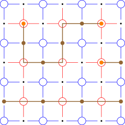
Figure 14: The figure illustrate an example of $\hat{f}_{1}$. The brown dots are the support of $\hat{f}_{1}$. The orange dots are the violated checks, i.e. the support of $\delta_{1}\hat{f}_{1}|_{\textnormal{int}}$. The graph consist of edges connecting the support of $\hat{f}_{1}$ with the nearby checks. We see that the graph decomposes into disjoint $\hat{f}_{1,i}$.

Step 1: Decompose $\hat{f}_{1}$ into components.

The goal of this step is to write $\hat{f}_{1}=\sum_{i}\hat{f}_{1,i}$ where $\operatorname{supp}\hat{f}_{1}$ is a disjoint union of $\operatorname{supp}\hat{f}_{1,i}$. Additionally, the support of $\hat{f}_{1,i}$ will look like 1d paths which will be made precise later.

To obtain the decomposition, we consider the (bipartite) graph consisting of edges formed by the active qubits in $\operatorname{supp}\hat{f}_{1}$ and their nearby checks. We call a check an active check if it is next to an active qubit. We see that a non-violated check has an even degree while a violated check has an odd degree. See Figure 14. Based on this structure of the graph, we can decompose the graph into components whose end points are the violated checks or boundary qubits and whose active check has degree at most two. Note that when a check has more than two neighboring active qubits, there is more than one possible decomposition satisfying the above properties. In such cases, any such decomposition works. Notice that when the component does not contain qubits on the seam, the component is either a 1d loop or a 1d path which are simple objects to analyze directly.

To be more mathematical, we can write $\hat{f}_{1}=\sum_{i}\hat{f}_{1,i}$ where $\{\hat{f}_{1,i}\}_{i}$ (the active qubits) have disjoint supports and $\{\delta_{1}\hat{f}_{1,i}|_{\textnormal{int}}\}_{i}$ (the violated checks) have disjoint supports. Furthermore, for each $\hat{f}_{1,i}$:

• The graph formed by the qubits and their neighboring checks, $\{(v,w)\in X(1)\times X(2):v\in\operatorname{supp}\hat{f}_{1,i},v\text{ is adjacent to }w\}$, is connected.

• Each check $w$ in the graph has degree at most two.

An example of the decomposition is illustrated in Figure 14(a).

Note that to find $f_{1}$, it suffices to find $f_{1,i}$ for each $\hat{f}_{1,i}$. This is because once given $f_{1,i}$, we can set $f_{1}=\sum_{i}f_{1,i}$. By construction, we have $f_{1}\in\hat{f}_{1}+B^{1}$ because $f_{1,i}\in\hat{f}_{1,i}+B^{1}$. The inequalities also carry over to $f_{i}$. For example, to show inequality (1) in Equation 31, we have

$$|f_{1}|\leq\sum_{i}|f_{1,i}|\leq\sum_{i}|\hat{f}_{1,i}|=|\hat{f}_{1}|$$ (47)

where the first inequality holds by the triangle inequality, the second inequality, $|f_{1,i}|\leq|\hat{f}_{1,i}|$, is based on the reduced problem for $\hat{f}_{1,i}$, and the third inequality holds because $\{\hat{f}_{1,i}\}_{i}$ have disjoint supports. Inequalities (2) and (3) in Equation 31 can be obtained similarly using the fact that $\{\delta_{1}\hat{f}_{1,i}|_{\textnormal{int}}\}_{i}$ have disjoint supports.

Step 2: Bound each component.

We now find $f_{1,i}$ for four different cases of $\hat{f}_{1,i}$. The last case is the hardest.

Case 1: The cluster has no violated check, i.e. $\delta_{1}\hat{f}_{1,i}=0$.

In this case, one can simply set $f_{1,i}=0$ which satisfies (1), (2), and (3).

Case 2: The cluster is not connected to the boundary nor the seam (excluding Case 1).

The corresponding graph of $\hat{f}_{1,i}$ is a path that connects two violated checks. We can set $f_{1,i}$ to be a shortest path between the two violated checks, for example, the path that goes vertically then horizontally.

We now check (1), (2), and (3). Inequality (1) is satisfied because $f_{1,i}$ is the vector with the smallest weight in $\hat{f}_{1,i}+B^{1}$. Inequality (2) holds because $|f_{1,i}|\leq L$ and $|\delta_{1}\hat{f}_{1,i}|_{\textnormal{int}}=2$. Inequality (3) holds because $|\delta_{1}f_{1,i}|_{\partial}=0$. (In particular, the inequalities hold whenever $\beta_{1}\leq\frac{2}{L}$.)

Case 3: The cluster is connected to the boundary but not the seam (excluding Case 1).

The corresponding graph of $\hat{f}_{1,i}$ is a path that connects one violated check and the boundary. We can set $f_{1,i}$ to be a shortest path between the violated check and the boundary which either goes up vertically or right horizontally.

We now check (1), (2), and (3). Inequality (1) is satisfied because $f_{1,i}$ is the vector with the smallest weight in $\hat{f}_{1,i}+B^{1}$. Inequality (2) holds because $|f_{1,i}|\leq L/2$ and $|\delta_{1}\hat{f}_{1,i}|_{\textnormal{int}}=1$. Inequality (3) holds because $|\delta_{1}^{\prime}f_{1,i}|_{\partial}=|\delta_{1}\hat{f}_{1,i}|_{\textnormal{int}}=1$ (In particular, the inequalities hold whenever $\beta_{1}\leq\frac{2}{L},\eta_{1}\leq 1$.)

Case 4: Otherwise, the cluster is connected to the seam.

The corresponding graph of $\hat{f}_{1,i}$ is more complicated, so we cannot apply structure results directly as above. What we do here is to reduce $\hat{f}_{1,i}$ to another vector $\hat{f}_{1,i}^{\prime}$ that is supported next to the seam. (The region next to the seam is depicted in Figure 15.) This is done by cleaning up the surface region using ideas similar to those in Case 1, 2, 3, and pushing the support next to but not past the seam. Vector $\hat{f}_{1,i}^{\prime}$ will then be analyzed in the next step.

It is straightforward to check that the structure of the graph in the 2d area is either:

• A path that connects two qubits on the seam.

• A path that connects one qubit on the seam and a violated check.

• A path that connects one qubit on the seam and the boundary.

This allows us to decompose $\hat{f}_{1,i}$ into $\hat{f}_{1,i}=\hat{f}_{1,i}^{x}+\sum_{j}\hat{f}_{1,i,j}^{y}+\sum_{k}\hat{f}_{1,i,k}^{z}+\sum_{l}\hat{f}_{1,i,l}^{w}$ with disjoint support where

• $\hat{f}_{1,i}^{x}$ is supported on the seam.

• $\hat{f}_{1,i,j}^{y}$ are the parts that connect two qubits on the seam.

• $\hat{f}_{1,i,k}^{z}$ are the parts that connect one qubit on the seam to the boundary.

• $\hat{f}_{1,i,l}^{w}$ are the parts that connect one qubit on the seam to a violated check.

Furthermore, $\{|\delta_{1}f_{1,i,k}^{z}|_{\partial}\}_{k}$ are disjoint and $\{|\delta_{1}f_{1,i,l}^{w}|_{\textnormal{int}}\}_{l}$ are disjoint.

We now simplify $\hat{f}_{1,i,j}^{y},\hat{f}_{1,i,k}^{z},\hat{f}_{1,i,l}^{w}$ into $f_{1,i,j}^{y},f_{1,i,k}^{z},f_{1,i,l}^{w}$ within the same homology, i.e. $g_{1}\in\hat{g}_{1}+B^{1}$ for $g_{1}$ being $f_{1,i,j}^{y}$, $f_{1,i,k}^{z}$, or $f_{1,i,l}^{w}$. Additionally, we have bound on weights $|g_{1}|\leq|\hat{g}_{1}|$.

• For $\hat{f}_{1,i,j}^{y}$, we simplify it into $f_{1,i,j}^{y}$ which connects the same two qubit through the route next to the seam.

• For $\hat{f}_{1,i,k}^{z}$, we simplify it into $f_{1,i,k}^{z}$ which is the shortest path between the qubit and the boundary. This path is next to the seam.

• For $\hat{f}_{1,i,l}^{w}$, we simplify it into $f_{1,i,l}^{w}$ which is the shortest path between the qubit and the violated check.

Let $\hat{f}_{1,i}^{\prime}=\hat{f}_{1,i}^{x}+\sum_{j}f_{1,i,j}^{y}+\sum_{k}f_{1,i,k}^{z}$. By construction $\hat{f}_{1,i}^{\prime}$ is supported next to the seam.

We claim that we can reduce the question of finding $f_{1,i}$ to the question of finding $f_{1,i}^{\prime}$ for $\hat{f}_{1,i}^{\prime}$ which will satisfy the inequalities

$$(1)\,|f_{1,i}^{\prime}|_{\textnormal{int}}\leq|\hat{f}_{1,i}^{\prime}|_{\textnormal{int}},\quad(2)\,\frac{2}{L}|f_{1,i}^{\prime}|_{\textnormal{int}}\leq|\delta_{1}\hat{f}_{1,i}^{\prime}|_{\textnormal{int}},\quad(3)\,\frac{1}{2}|\delta_{1}f_{1,i}^{\prime}|_{\partial}\leq|\delta_{1}\hat{f}_{1,i}^{\prime}|_{\textnormal{int}}.$$ (48)

The reason is that suppose we have $f_{1,i}^{\prime}\in\hat{f}_{1,i}^{\prime}+B^{1}$, we can then set $f_{1,i}=f_{1,i}^{\prime}+\sum_{l}f_{1,i,l}^{w}$. One can straightforwardly check that $f_{1,i}\in\hat{f}_{1,i}+B^{1}$.

We now check inequalities (1), (2), and (3) in Equation 31. Inequality (1) holds because

$$|f_{1,i}| \leq|f_{1,i}^{\prime}|+\sum_{l}|f_{1,i,l}^{w}|$$

$$\leq|\hat{f}_{1,i}^{\prime}|+\sum_{l}|f_{1,i,l}^{w}|$$

$$\leq|\hat{f}_{1,i}^{x}|+\sum_{j}|f_{1,i,j}^{y}|+\sum_{k}|f_{1,i,k}^{z}|+\sum_{l}|f_{1,i,l}^{w}|$$

$$\leq|\hat{f}_{1,i}^{x}|+\sum_{j}|\hat{f}_{1,i,j}^{y}|+\sum_{k}|\hat{f}_{1,i,k}^{z}|+\sum_{l}|\hat{f}_{1,i,l}^{w}|$$

$$=|\hat{f}_{1,i}|$$

where the last equality holds because the components are disjoint.

Inequality (2) holds for $\beta_{1}=\frac{2}{3L}$ because

$$|f_{1,i}|\leq|f_{1,i}^{\prime}|+\sum_{l}|f_{1,i,l}^{w}|\leq\frac{L}{2}|\delta_{1}\hat{f}_{1,i}^{\prime}|_{\textnormal{int}}+\sum_{l}L\leq\left(\frac{L}{2}+L\right)|\delta_{1}\hat{f}_{1,i}|_{\textnormal{int}}.$$

The second inequality uses $|f_{1,i,l}^{w}|\leq L$. The third inequality uses $|\delta_{1}\hat{f}_{1,i}^{\prime}|_{\textnormal{int}}=|\delta_{1}\hat{f}_{1,i}|_{\textnormal{int}}$ and $\sum_{l}1=|\delta_{1}\hat{f}_{1,i}|_{\textnormal{int}}$.

Inequality (3) holds for $\eta_{1}=\frac{1}{2}$ because

$$|\delta_{1}f_{1,i}|_{\partial}=|\delta_{1}f_{1,i}^{\prime}|_{\partial}\leq 2|\delta_{1}\hat{f}_{1,i}|_{\textnormal{int}}=2|\delta_{1}\hat{f}_{1,i}|_{\textnormal{int}}.$$

The remaining task is to find $f_{1,i}^{\prime}$ for $\hat{f}_{1,i}^{\prime}$ that is supported next to the seam.

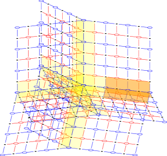
Figure 15: The figure illustrate the regions next to the seam in yellow. Each orange region will be referred to as a limb.

Step 3: Show the case where $\hat{f}_{1,i}^{\prime}$ is next to the seam.

We simply pick $f_{1,i}^{\prime}$ to be the vector with the smallest weight in $\hat{f}_{1,i}^{\prime}+B^{1}$ while being next to the seam. This automatically satisfies inequality (1) in Equation 48.

For inequality (2) in Equation 48, we construct a vector $f_{1,i}^{\prime\prime}\in\hat{f}_{1,i}^{\prime}+B^{1}$ with $\frac{2}{L}|f_{1,i}^{\prime\prime}|_{\textnormal{int}}\leq|\delta_{1}\hat{f}_{1,i}^{\prime}|_{\textnormal{int}}$. Since $f_{1,i}^{\prime}$ has the smallest weight, it implies inequality (2). One can simply construct $f_{1,i}^{\prime\prime}$ by connecting each violated check, i.e. $\operatorname{supp}\delta_{1}\hat{f}_{1,i}^{\prime}$ to the closest boundary. Since each point is at most $\frac{L-1}{2}$ distance away from the boundary, we have $|f_{1,i}^{\prime\prime}|_{\textnormal{int}}\leq\frac{L-1}{2}|\delta_{1}\hat{f}_{1,i}^{\prime}|_{\textnormal{int}}\leq\frac{L}{2}|\delta_{1}\hat{f}_{1,i}^{\prime}|_{\textnormal{int}}$. (We need the tighter bound $|f_{1,i}^{\prime\prime}|_{\textnormal{int}}\leq\frac{L-1}{2}|\delta_{1}\hat{f}_{1,i}^{\prime}|_{\textnormal{int}}$ in the next paragraph.)

For inequality (3) in Equation 48, to show $\frac{1}{2}|\delta_{1}f_{1,i}^{\prime}|_{\partial}\leq|\delta_{1}\hat{f}_{1,i}^{\prime}|_{\textnormal{int}}$, we use proof by contradiction. We assume $|\delta_{1}f_{1,i}^{\prime}|_{\partial}>2|\delta_{1}\hat{f}_{1,i}^{\prime}|_{\textnormal{int}}$ and show that $f_{1,i}^{\prime}$ is not the vector in $\hat{f}_{1,i}^{\prime}+B^{1}$ with the smallest weight. In particular, we will show $|f_{1,i}^{\prime}|>\frac{L-1}{2}|\delta_{1}\hat{f}_{1,i}^{\prime}|_{\textnormal{int}}$. Because $|f_{1,i}^{\prime\prime}|\leq\frac{L-1}{2}|\delta_{1}\hat{f}_{1,i}^{\prime}|_{\textnormal{int}}$ from the last paragraph, $f_{1,i}^{\prime}$ has a larger weight than $f_{1,i}^{\prime\prime}$ which is the contradiction.

We first perform some basic structural analysis of $f_{1,i}^{\prime}$ then observe a local condition of $f_{1,i}^{\prime}$. Consider $v\in\operatorname{supp}f_{1,i}^{\prime}$ on a horizontal seam. We study the corresponding limb as illustrated in Figure 15. The edges emanating from $v$ either end at the neighboring violated check, or go towards the center, or go towards the boundary. Let the number of edges of each type be $p,q,r$, respectively. We claim that $p,q,r$ satisfies $p+q\geq r$. Otherwise, if $p+q<r$, and one can replace $f_{1,i}^{\prime}$ with $f_{1,i}^{\prime}+\delta_{0}1_{w}$, where $w$ is the stabilizer next to the qubit $v$ that is closer to the boundary. See Figure 16(a)(b) for an illustration.

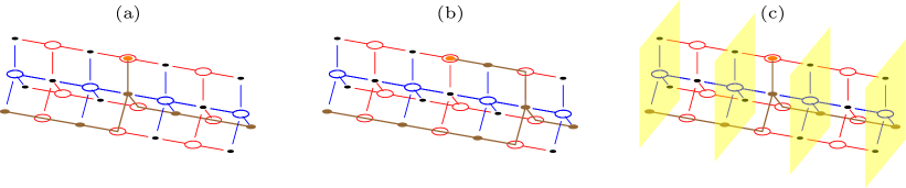
Figure 16: The figure illustrates one of the limbs where left is the direction to the center and right is the direction to the boundary. (a) The minimal vector $f_{1,i}^{\prime}$. (b) The new vector $f_{1,i}^{\prime}+\delta_{0}1_{w}$ which has a lower weight if $p+q<r$. (c) The cross sections.

We now use the local condition $p+q\geq r$ and the assumption $|\delta_{1}f_{1,i}^{\prime}|_{\partial}>2|\delta_{1}\hat{f}_{1,i}^{\prime}|_{\textnormal{int}}$ to show $|f_{1,i}^{\prime}|>\frac{L-1}{2}|\delta_{1}\hat{f}_{1,i}^{\prime}|_{\textnormal{int}}$. Consider one of the limbs. Suppose the limb contains $s$ violated checks and $t$ lines that connect to the boundary. Consider the number of active qubits on each cross section as shown in Figure 16(c). We claim that this number is at least $t-s$ for each cross section. Assuming so, since there are $\frac{L-1}{2}$ cross sections, this limb contains at least $\frac{L-1}{2}(t-s)$ active qubits, i.e. $|\operatorname{supp}f_{1,i}^{\prime}\cap M|\geq\frac{L-1}{2}(t-s)$ where $M$ is the set of vertices on the limb. We apply this observation to all limbs. Because the total number of violated checks is at most $|\delta_{1}\hat{f}_{1,i}^{\prime}|_{\textnormal{int}}$ and the number of lines that connect to the boundary is $|\delta_{1}f_{1,i}^{\prime}|_{\partial}$, this means the number of active qubits $|f_{1,i}^{\prime}|$ is at least $\frac{L-1}{2}(|\delta_{1}f_{1,i}^{\prime}|_{\partial}-|\delta_{1}\hat{f}_{1,i}^{\prime}|_{\textnormal{int}})>\frac{L-1}{2}|\delta_{1}\hat{f}_{1,i}^{\prime}|_{\textnormal{int}}$. It suffices to show the claim.

Notice the number of active qubits on the cross section changes only when there is an active qubit on the seam between the two cross sections. With the same notation $p,q,r$, this number changes from $r$ to $q$ as we go closer to the center. The number drops by at most $p$ because the local condition says $q\geq r-p$. Since the number of active qubits is $t$ on the cross section closest to boundary and the number drops by at most $s$, each cross section has at least $t-s$ active qubits. ∎

6 Application to Classical Codes

The main part of the paper discusses the construction based on quantum LDPC codes. This section explores the implications when applying the techniques to classical LDPC codes and shows Theorem 1.3.

6.1 Code Construction

Given a classical LTC [1, 34, 38, 17, 18], let $\mathbb{F}_{2}^{X(0)}\to\mathbb{F}_{2}^{X(1)}$ be the parity-check matrix where $X(0)$ are the bits and $X(1)$ are the checks. The code naturally corresponds to the adjacency matrix of a bipartite graph $\mathcal{G}$ with vertices $V(\mathcal{G})=X(0)\cup X(1)$. We can subdivide both the code and the graph as shown in Figure 17. We denote $X_{L}$ as the subdivided code and $\mathcal{G}_{L}$ as the subdivided graph.

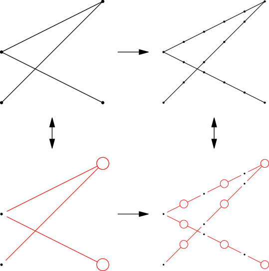
Figure 17: The subdivision of a classical LTC $X$ together with the subdivision of the associated bipartite graph $\mathcal{G}$.

The embedding of the code again boils down to the embedding of the subdivided graph which is known.

Theorem 6.1 (Modified [6, Theorem 7]).

Given a bounded degree graph $\mathcal{G}$, the $L$-subdivision $\mathcal{G}_{L}$ has an embedding $f:V(\mathcal{G}_{L})\to\mathbb{Z}^{D}$ with constant $a,b=\Theta(1)$ such that

1. Geometrically local: For all adjacent vertices on the complex $(v_{0},v_{1})\in E(\mathcal{G}_{L})$, the distance of corresponding points in $\mathbb{Z}^{D}$ is bounded $|f(v_{0})-f(v_{1})|\leq a$.

2. Bounded density: The number of vertices at each point is bounded, i.e. for all $x\in\mathbb{Z}^{D}$, $|f^{-1}(x)|\leq b$.

for $L=|V(\mathcal{G})|^{\frac{1}{D-1}}\log^{D+1}|V(\mathcal{G})|$.

Remark 6.2.

When $D=3$, Kolmogorov and Barzdin [43] gave the optimal local embedding of expander graphs without polylogs $L=\Theta(|V(\mathcal{G}|^{\frac{1}{2}}))$. We will show that an embedding without polylogs can also be established for all $D\geq 2$ in a future paper.

6.2 Code Properties

It is clear that the code has a geometrically local embedding induced from the graph. So we will mainly focus on the non geometric properties, including code dimension, distance, energy barrier, and soundness.

Similar to Section 3.2, we define the chain map $\mathcal{F}$, which maps the original LTC $\mathbb{F}_{2}^{X(0)}\to\mathbb{F}_{2}^{X(1)}$ to the subdivided LTC $\mathbb{F}_{2}^{X_{L}(0)}\to\mathbb{F}_{2}^{X_{L}(1)}$. This utilizes the bijection between vertices and connected components depicted in Figure 18 where $\mathcal{T}$ and $\mathcal{U}$ are the sets of connected components of $T$ and $U$.

• Given $\widetilde{c}_{0}\in\mathbb{F}_{2}^{X(0)}$, we define $\mathcal{F}_{0}(\widetilde{c}_{0})\in\mathbb{F}_{2}^{X_{L}(0)}$ by repeating the value $\widetilde{c}_{0}(v)$ at the corresponding component $T_{i}$ of $v$ for each $v\in X(0)$.

• Given $\widetilde{c}_{1}\subset\mathbb{F}_{2}^{X(1)}$, we define $\mathcal{F}_{1}(\widetilde{c}_{1})\in\mathbb{F}_{2}^{X_{L}(1)}$ by setting the value $\widetilde{c}_{1}(v)$ at the corresponding vertex $U_{i}$ of $v$ for each $v\in X(1)$ and set other values in $T$ to be $0$.

The maps form the following commutative diagram.

(49)

Figure 18: Regions $T,U$ and the bijections $X(0)\cong\mathcal{T}$, $X(1)\cong\mathcal{U}$.

The following lemma relates the code properties of the original code $C(X)$ and the subdivided code $C(X_{L})$.

Lemma 6.3.

If the code $C(X)$ has dimension $k_{\textnormal{LTC}}$ then the code $C(X_{L})$ has dimension $k=k_{\textnormal{LTC}}$.

If the code $C(X)$ has distance $d_{\textnormal{LTC}}$ then the code $C(X_{L})$ has distance $d\geq L\,d_{\textnormal{LTC}}$.

If the code $C(X)$ has soundness $s_{\textnormal{LTC}}$ then the code $C(X_{L})$ has soundness

$$s\geq\frac{|X_{L}(0)|}{|X_{L}(1)|}\frac{1}{\frac{1}{\beta^{\textnormal{rep}}}+\frac{1}{\eta^{\textnormal{rep}}}\frac{|X(0)|}{|X(1)|}\frac{1}{s_{\textnormal{LTC}}}\frac{\Delta_{\max}}{2}L}.$$ (50)

In our context $\beta^{\textnormal{rep}}=\Theta(1/L)$, $\eta^{\textnormal{rep}},\Delta_{\max}=\Theta(1)$, $|X_{L}(0)|=\Theta(L|X(0)|)$, and $|X_{L}(1)|=\Theta(L|X(1)|)$. Therefore, when $X$ is chosen to be the LTC with linear dimension, linear distance, constant soundness, and satisfies $|X(1)|=\Theta(|X(0)|)$ provided in [16, 34, 38, 17, 18], $X_{L}$ gives the desired properties Theorem 1.3. (Recall the bound on energy barrier can be inferred from the bound on distance and soundness as discussed in Section 2.2.)

The lemma can be derived using similar arguments as those presented in Section 4. Here, we provide only a proof sketch for code dimension and distance. The code dimension of $C(X_{L})$ can be estabilished by showing $\mathcal{F}_{0}$ induces a bijection between the codewords of $C(X)$ and $C(X_{L})$. The distance of $C(X_{L})$ can be shown by using this bijection and the fact that all bits in a component $T_{i}$ take the same value where $T_{i}$ has size at least $L$.

We now discuss the proof of soundness.

Proof of soundness.

The goal is to show that for each $c_{0}\in\mathbb{F}_{2}^{X_{L}(0)}$, there exists a codeword $h_{0}\in Z^{0}(X_{L})$ such that

$$\frac{s}{|X_{L}(0)|}|c_{0}-h_{0}|\leq\frac{1}{|X_{L}(1)|}|\delta_{0}c_{0}|.$$ (51)

The idea is to apply the coboundary expansion of the generalized repetition code to replace $c_{0}$ with $c_{0}^{\prime}$ which is in the image of $\mathcal{F}_{0}$. We then move back to the original code with $\widetilde{c}_{0}=\mathcal{F}_{0}^{-1}(c_{0}^{\prime})\in\mathbb{F}_{2}^{X(0)}$. This allows us to apply the soundness property of $X$ to find a codeword $\widetilde{h}_{0}\in Z^{0}(X)$. The codeword $\widetilde{h}_{0}$ then induces the codeword $h_{0}=\mathcal{F}_{0}(\widetilde{h}_{0})\in Z^{0}(X_{L})$ which we claim to satisfy the desired inequaliy, Equation 51.

Step 1: Construct $c_{0}^{\prime}$ by making $c_{0}$ consistent in $T$.

By applying Corollary 5.4 to the disjoint regions of $T$ with $\hat{f}_{0}=c_{0}$, there exist $c_{0}^{T}=f_{0}$ supported on $T$ which satisfies

$$(a)\,c_{0}+c^{T}_{0}\in B^{0},\quad(b)\,|c^{T}_{0}|_{T}\leq|c_{0}|_{T},\quad(c)\,\beta^{\textnormal{rep}}|c^{T}_{0}|_{T}\leq|\delta_{0}c_{0}|_{T},\quad(d)\,\eta^{\textnormal{rep}}|\delta_{0}c^{T}_{0}|_{U}\leq|\delta_{0}c_{0}|_{T}.$$ (52)

We set $c_{0}^{\prime}=c_{0}+c^{T}_{0}$ which by (a) violates no check in $T$, i.e. consistent in $T$.

Notice

$$|\delta_{0}c_{0}^{\prime}|=|\delta_{0}c_{0}^{\prime}|_{U}\leq|\delta_{0}c_{0}^{T}|_{U}+|\delta_{0}c_{0}|_{U}\leq\frac{1}{\eta^{\textnormal{rep}}}|\delta_{0}c_{0}|_{T}+|\delta_{0}c_{0}|_{U}\leq\frac{1}{\eta^{\textnormal{rep}}}|\delta_{0}c_{0}|$$ (53)

where the third inequality uses (d) and the last inequality uses $1\leq\frac{1}{\eta^{\textnormal{rep}}}$.

Step 2: Construct $\widetilde{c}_{0}$ from $c_{0}^{\prime}$ by moving from $X_{L}$ to $X$.

The consistency of $c_{0}^{\prime}$ implies $c_{0}^{\prime}\in\operatorname{im}\mathcal{F}_{0}$. Therefore, we define $\widetilde{c}_{0}=\mathcal{F}_{0}^{-1}c_{0}^{\prime}$.

Notice

$$|\delta_{0}c_{0}^{\prime}|=|\delta_{0}\mathcal{F}_{0}(\widetilde{c}_{0})|=|\mathcal{F}_{1}(\delta_{0}\widetilde{c}_{0})|=|\delta_{0}\widetilde{c}_{0}|$$ (54)

where the third equality holds because, by construction, $\mathcal{F}_{1}$ preserves the weight.

Step 3: Construct $\widetilde{h}_{0}$ from $\widetilde{c}_{0}$ by applying soundness assumption of $X$.

By soundness of $C(X)$, there exists $\widetilde{h}_{0}\in Z^{0}(X)$ such that

$$\frac{s_{\textnormal{LTC}}}{|X(0)|}|\widetilde{c}_{0}-\widetilde{h}_{0}|\leq\frac{1}{|X(1)|}|\delta_{0}\widetilde{c}_{0}|.$$ (55)

Step 4: Construct $h_{0}$ from $\widetilde{h}_{0}$ by moving back from $X$ to $X_{L}$.

Let $h_{0}=\mathcal{F}_{0}(\widetilde{h}_{0})$. By the commutative diagram Equation 49, this implies $h_{0}\in Z^{0}(X_{L})$ is a codeword.

Notice that

$$|c_{0}^{\prime}-h_{0}|=|\mathcal{F}_{0}(\widetilde{c}_{0}-\widetilde{h}_{0})|\leq\frac{\Delta_{\max}}{2}L|\widetilde{c}_{0}-\widetilde{h}_{0}|$$ (56)

because each entry in $\widetilde{c}_{0}-\widetilde{h}_{0}$ is repeated at most $\Delta_{\max}\frac{L-1}{2}+1\leq\frac{\Delta_{\max}}{2}L$ times.

Wrap up.

Finally, we show the inequality, Equation 51.

$$|c_{0}-h_{0}| =|-c_{0}^{T}+c_{0}^{\prime}-h_{0}|$$

$$\leq|c_{0}^{T}|+|c_{0}^{\prime}-h_{0}|$$

$$\leq\frac{1}{\beta^{\textnormal{rep}}}|\delta_{0}c_{0}|+\frac{\Delta_{\max}}{2}L|\widetilde{c}_{0}-\widetilde{h}_{0}|$$

$$\leq\frac{1}{\beta^{\textnormal{rep}}}|\delta_{0}c_{0}|+\frac{|X(0)|}{|X(1)|}\frac{1}{s_{\textnormal{LTC}}}\frac{\Delta_{\max}}{2}L|\delta_{0}\widetilde{c}_{0}|$$

$$=\frac{1}{\beta^{\textnormal{rep}}}|\delta_{0}c_{0}|+\frac{|X(0)|}{|X(1)|}\frac{1}{s_{\textnormal{LTC}}}\frac{\Delta_{\max}}{2}L|\delta_{0}c_{0}^{\prime}|$$

$$\leq\frac{1}{\beta^{\textnormal{rep}}}|\delta_{0}c_{0}|+\frac{1}{\eta^{\textnormal{rep}}}\frac{|X(0)|}{|X(1)|}\frac{1}{s_{\textnormal{LTC}}}\frac{\Delta_{\max}}{2}L|\delta_{0}c_{0}|$$

$$=\left(\frac{1}{\beta^{\textnormal{rep}}}+\frac{1}{\eta^{\textnormal{rep}}}\frac{|X(0)|}{|X(1)|}\frac{1}{s_{\textnormal{LTC}}}\frac{\Delta_{\max}}{2}L\right)|\delta_{0}c_{0}|$$ (57)

where the third inequality uses Equation 52(c) and Equation 56. The fourth inequality uses Equation 55. The fifth equality uses Equation 54. The sixth inequality uses Equation 53. ∎

Appendix A Upper Bound on Dimension, Distance, and Energy Barrier

This section collects various known upper bound on the geometrically local codes which our constructions have matched up to $\operatorname{polylog}(n)$. We assume the codes have at most $1$ qubit (bit) at each lattice site of $[L]^{D}$ where $[L]=\{0,1,2,...,L-1\}$.

We first discuss the bound on distance and energy barrier of the geometrically local quantum codes.

Theorem A.1 ([2, Theorem 1, 2]).

Suppose $L\geq 2(r-1)^{2}$. For geometrically local quantum codes in $[L]^{D}$

$$d\leq rL^{D-1},\quad\mathcal{E}\leq 6r^{2}L^{D-2}$$ (58)

where each stabilizer generator is bounded by a hypercube of size $r^{D}$.

Note that in [2, Theorem 2], although the authors did not state the case where the dimension is greater than $2$, the proof technique applies directly and yield the bound stated above.

The idea is that one can show the existence of a logical operator in a slab of width $r$, which implies $d\leq rL^{D-1}$. (The slab has width $r$ in one of the directions and length $L$ in the other $D-1$ directions) Then one can create this logical operator layer by layer (in one of the length $L$ directions). Only the end layer costs energy which gives $\mathcal{E}\leq 6r^{2}L^{D-2}$.

The same idea applies to classical codes.

Theorem A.2.

For geometrically local classical codes in $[L]^{D}$

$$d\leq L^{D},\quad\mathcal{E}\leq rL^{D-1}$$ (59)

where each check is bounded by a hypercube of size $r^{D}$.

We now discuss the tradeoff between code dimension and distance.

Theorem A.3 ([3, Equation 4, 5]).

For quantum codes

$$k\leq\frac{2Dr^{2}L^{D}}{\left(\frac{d}{2Dr}\right)^{\frac{2}{D-1}}}=\Theta\bigg{(}\frac{L^{D}}{d^{\frac{2}{D-1}}}\bigg{)}$$ (60)

for large enough $d$.

For classical codes

$$k\leq L^{D}\left(1-\frac{d}{\left(d^{\frac{1}{D}}+r\right)^{D}}\right)\leq\frac{DrL^{D}}{d^{\frac{1}{D}}}=\Theta\bigg{(}\frac{L^{D}}{d^{\frac{1}{D}}}\bigg{)}$$ (61)

for large enough where $d\geq r^{D}$.

We leave it as an open question about the tradeoff between code dimension and the energy barrier.

Appendix B A Subdivision of the Quantum LDPC Code by Leverrier and Zémor

This section discusses a subdivided code derived from the good quantum LDPC code constructed by Leverrier and Zémor [17] which we will refer to as the LZ code. The main challenge in constructing the subdivided code for the LZ code is that the LZ code likely cannot be viewed as a balanced product code. Nevertheless, we provide a “geometric realization” of the LZ code, similar to how the square complex relates to the balanced product code. Once we have this geometric realization, the subdivision process becomes transparent. We should note that this geometric realization differs somewhat from the language used when discussing square complexes. In fact, we will rephrase the geometric realization of the balanced product code to make them more similar.

We first briefly reivew the construction of the LZ code. The LZ code is a Tanner code built on top of the left-right Cayley compelx discussed in Section 2.3. Recall that the complex has four sets of vertices $V_{00},V_{10},V_{01},V_{11}$ and squares $F$. The code is obtain by putting qubits on $F$, X-checks on $V_{00}\cup V_{11}$, and Z-checks on $V_{01}\cup V_{10}$. When we geometrize the code, each of these elements corresponds to a 2-cell as depicted in Figure 19. As a comparison, the geometrization of the balanced product code is depicted in Figure 20.

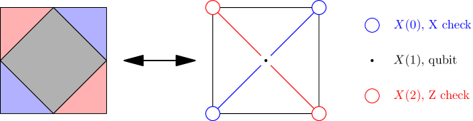
Figure 19: Geometrizing the LZ code.

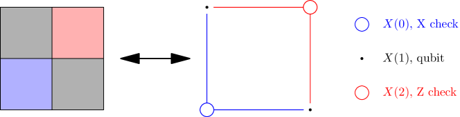
Figure 20: Geometrizing the balanced product code.

We can then construct the subdivided code by subdividing each of the 2-cell. Another way to say it is that we encode each element using a code similar to the surface code. The examples for the LZ code and the balanced product code are depicted in Figures 21 and 22.

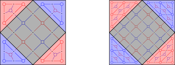
Figure 21: Subdividing the LZ code with various sizes.

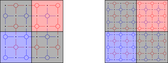
Figure 22: Subdividing the balanced product code with various sizes.

Notice that the boundary structure of the surface codes can be categorized into two types. It either consists of qubits and Z checks or qubits and X checks, which we will refer to as the “red type” and the “blue type”. We observe that the boudnary of a red 2-cell is of the red type, while the boundary of a blue 2-cell is of the blue type. For the black 2-cell, the type of the boundary follows a specific pattern. When an edge is next to a red cell, it is of the blue type, whereas if it is next to a blue cell, it is of the red type. This arrangement implies the subdivied code remains to be a chain complex.

It is plausible that the subdivided code of the LZ code has the same good properties as the subdivided code of the balanced product code. We leave the analysis as an open direction.

References

• [1] Pavel Panteleev and Gleb Kalachev. Asymptotically good quantum and locally testable classical ldpc codes. arXiv preprint arXiv:2111.03654, 2021.
• [2] Sergey Bravyi and Barbara Terhal. A no-go theorem for a two-dimensional self-correcting quantum memory based on stabilizer codes. New Journal of Physics, 11(4):043029, 2009.
• [3] Sergey Bravyi, David Poulin, and Barbara Terhal. Tradeoffs for reliable quantum information storage in 2d systems. Physical review letters, 104(5):050503, 2010.
• [4] Jeongwan Haah. Local stabilizer codes in three dimensions without string logical operators. Physical Review A, 83(4):042330, 2011.
• [5] Kamil P Michnicki. 3d topological quantum memory with a power-law energy barrier. Physical review letters, 113(13):130501, 2014.
• [6] Elia Portnoy. Local quantum codes from subdivided manifolds. arXiv preprint arXiv:2303.06755, 2023.
• [7] Michael Freedman and Matthew Hastings. Building manifolds from quantum codes. Geometric and Functional Analysis, 31(4):855–894, 2021.
• [8] Misha Gromov and Larry Guth. Generalizations of the kolmogorov–barzdin embedding estimates. 2012.
• [9] Nikolas P Breuckmann and Jens N Eberhardt. Balanced product quantum codes. IEEE Transactions on Information Theory, 67(10):6653–6674, 2021.
• [10] A Yu Kitaev. Fault-tolerant quantum computation by anyons. Annals of Physics, 303(1):2–30, 2003.
• [11] Jean-Pierre Tillich and Gilles Zémor. Quantum ldpc codes with positive rate and minimum distance proportional to the square root of the blocklength. IEEE Transactions on Information Theory, 60(2):1193–1202, 2013.
• [12] Michael H Freedman, David A Meyer, and Feng Luo. Z2-systolic freedom and quantum codes. In Mathematics of quantum computation, pages 303–338. Chapman and Hall/CRC, 2002.
• [13] Shai Evra, Tali Kaufman, and Gilles Zémor. Decodable quantum ldpc codes beyond the square root distance barrier using high dimensional expanders. arXiv preprint arXiv:2004.07935, 2020.
• [14] Tali Kaufman and Ran J Tessler. New cosystolic expanders from tensors imply explicit quantum ldpc codes with $\Omega(\sqrt{n}\log^{k}n)$ distance. arXiv preprint arXiv:2008.09495, 2020.
• [15] Matthew B Hastings, Jeongwan Haah, and Ryan O’Donnell. Fiber bundle codes: breaking the n 1/2 polylog (n) barrier for quantum ldpc codes. In Proceedings of the 53rd Annual ACM SIGACT Symposium on Theory of Computing, pages 1276–1288, 2021.
• [16] Pavel Panteleev and Gleb Kalachev. Quantum ldpc codes with almost linear minimum distance. IEEE Transactions on Information Theory, 68(1):213–229, 2022.
• [17] Anthony Leverrier and Gilles Zémor. Quantum tanner codes. arXiv preprint arXiv:2202.13641, 2022.
• [18] Irit Dinur, Min-Hsiu Hsieh, Ting-Chun Lin, and Thomas Vidick. Good quantum ldpc codes with linear time decoders. arXiv preprint arXiv:2206.07750, 2022.
• [19] Shouzhen Gu, Christopher A Pattison, and Eugene Tang. An efficient decoder for a linear distance quantum ldpc code. arXiv preprint arXiv:2206.06557, 2022.
• [20] Anthony Leverrier and Gilles Zémor. Efficient decoding up to a constant fraction of the code length for asymptotically good quantum codes. arXiv preprint arXiv:2206.07571, 2022.
• [21] Anthony Leverrier and Gilles Zémor. A parallel decoder for good quantum ldpc codes. arXiv preprint arXiv:2208.05537, 2022.
• [22] Max Hopkins and Ting-Chun Lin. Explicit lower bounds against $\omega(n)$-rounds of sum-of-squares. arXiv preprint arXiv:2204.11469, 2022.
• [23] Anurag Anshu, Nikolas Breuckmann, and Chinmay Nirkhe. Nlts hamiltonians from good quantum codes. arXiv preprint arXiv:2206.13228, 2022.
• [24] Eric Dennis, Alexei Kitaev, Andrew Landahl, and John Preskill. Topological quantum memory. Journal of Mathematical Physics, 43(9):4452–4505, 2002.
• [25] Sergey Bravyi and Jeongwan Haah. Energy landscape of 3d spin hamiltonians with topological order. Physical review letters, 107(15):150504, 2011.
• [26] Beni Yoshida. Information storage capacity of discrete spin systems. Annals of Physics, 338:134–166, 2013.
• [27] Courtney G Brell. A proposal for self-correcting stabilizer quantum memories in 3 dimensions (or slightly less). New Journal of Physics, 18(1):013050, 2016.
• [28] Guanyu Zhu, Tomas Jochym-O’Connor, and Arpit Dua. Topological order, quantum codes, and quantum computation on fractal geometries. PRX Quantum, 3(3):030338, 2022.
• [29] Jeongwan Haah. A degeneracy bound for homogeneous topological order. SciPost Physics, 10(1):011, 2021.
• [30] Robert Alicki, Michal Horodecki, Pawel Horodecki, and Ryszard Horodecki. On thermal stability of topological qubit in kitaev’s 4d model. Open Systems & Information Dynamics, 17(01):1–20, 2010.
• [31] Self-correcting quantum code. In Victor V. Albert and Philippe Faist, editors, The Error Correction Zoo. 2022.
• [32] Ting-Chun Lin and Min-Hsiu Hsieh. Good quantum ldpc codes with linear time decoder from lossless expanders. arXiv preprint arXiv:2203.03581, 2022.
• [33] Bruce W Jordan and Ron Livné. The ramanujan property for regular cubical complexes. 2000.
• [34] Irit Dinur, Shai Evra, Ron Livne, Alexander Lubotzky, and Shahar Mozes. Locally testable codes with constant rate, distance, and locality. arXiv preprint arXiv:2111.04808, 2021.
• [35] Nathan Linial and Roy Meshulam. Homological connectivity of random 2-complexes. Combinatorica, 26(4):475–487, 2006.
• [36] Yotam Dikstein and Irit Dinur. Coboundary and cosystolic expansion without dependence on dimension or degree. arXiv preprint arXiv:2304.01608, 2023.
• [37] Kitaev surface code. In Victor V. Albert and Philippe Faist, editors, The Error Correction Zoo. 2023.
• [38] Ting-Chun Lin and Min-Hsiu Hsieh. $c^{3}$-local testable codes from lossless expanders. arXiv preprint arXiv:2201.11369, 2022.
• [39] Fan RK Chung and Prasad Tetali. Isoperimetric inequalities for cartesian products of graphs. Combinatorics, Probability and Computing, 7(2):141–148, 1998.
• [40] Jean-Pierre Tillich. Edge isoperimetric inequalities for product graphs. Discrete Mathematics, 213(1-3):291–320, 2000.
• [41] Dominique Bakry, Ivan Gentil, Michel Ledoux, et al. Analysis and geometry of Markov diffusion operators, volume 103. Springer, 2014.
• [42] Ryan O’Donnell. Analysis of boolean functions. Cambridge University Press, 2014.
• [43] Ya M Barzdin. On the realization of networks in three-dimensional space. Selected Works of AN Kolmogorov: Volume III: Information Theory and the Theory of Algorithms, pages 194–202, 1993.