Rapid Network Adaptation:
Learning to Adapt Neural Networks Using Test-Time Feedback

Abstract

We propose a method for adapting neural networks to distribution shifts at test-time. In contrast to training-time robustness mechanisms that attempt to anticipate and counter the shift, we create a closed-loop system and make use of a test-time feedback signal to adapt a network on the fly. We show that this loop can be effectively implemented using a learning-based function, which realizes an amortized optimizer for the network. This leads to an adaptation method, named Rapid Network Adaptation (RNA), that is notably more flexible and orders of magnitude faster than the baselines. Through a broad set of experiments using various adaptation signals and target tasks, we study the efficiency and flexibility of this method. We perform the evaluations using various datasets (Taskonomy, Replica, ScanNet, Hypersim, COCO, ImageNet), tasks (depth, optical flow, semantic segmentation, classification), and distribution shifts (Cross-datasets, 2D and 3D Common Corruptions) with promising results. We end with a discussion on general formulations for handling distribution shifts and our observations from comparing with similar approaches from other domains.

1 Introduction

Neural networks are found to be unreliable against distribution shifts [23, 37, 48, 46, 30]. Examples of such shifts include blur due to camera motion, object occlusions, changes in weather conditions and lighting, etc. The training-time strategies to deal with this issue attempt to anticipate the shifts that may occur and counter them at the training stage – for instance, by augmenting the training data or updating the architecture with corresponding robustness inductive biases. As the possible shifts are numerous and unpredictable, this approach has inherent limitations. This is the main motivation behind test-time adaptation methods, which instead aim to adapt to such shifts as they occur and recover from failure. In other words, these methods choose adaptation over anticipation (see Fig. 1). In this work, we propose a test-time adaptation framework that aims to perform an efficient adaptation of a given main network using a feedback signal.

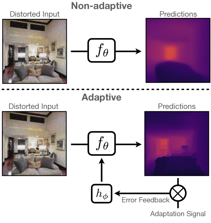
Figure 1: Adaptive vs non-adaptive neural network pipelines. Top: In order to be robust, non-adaptive methods include training-time interventions that anticipate and counter the distribution shifts that will occur at test-time (e.g., via data augmentation). The learned model, $f_{\theta}$, is frozen at test-time, thus upon encountering an out-of-distribution input, its predictions may collapse. Bottom: Adaptive methods create a closed-loop and use an adaptation signal at test-time. The adaptation signal is a quantity that can be computed at test-time from the environment. $h_{\phi}$ acts as a “controller” by taking in an error feedback, computed from the adaptation signal and model predictions, to adapt $f_{\theta}$ accordingly. It can be implemented as a (i) standard optimizer (e.g., using SGD) or (ii) neural network. The former is equivalent to test-time optimization (TTO), while the latter aims to amortize the optimization process, by training a controller network to adapt $f_{\theta}$ – thus, it can be more efficient and flexible. In this work, we study the latter approach and show its efficiency and flexibility.

One can consider performing “test-time optimization” (TTO) for this purpose, similar to previous works [100, 117, 28]. This involves using SGD to finetune the network to reduce a proxy loss. While this can successfully adapt a network, it is unnecessarily inefficient as it does not make use of the learnable regularities in the adaptation process, and consequently, unconducive for real-world applications. It also results in a rigid framework as the update mechanism is fixed to be the same as the training process of neural networks (SGD). We show this process can be effectively amortized using a learning-based feed-forward controller network, which yields orders of magnitude faster results (See Fig. 1, Sec. 4.3). In addition, it provides flexibility advantages as the controller is implemented using a neural network and can be engineered to include arbitrary inductive biases and desired features that could counter the suboptimalities of the adaptation signal.

2 Related Work

Our work focuses on how to adapt a neural network in an efficient way at test-time on a range tasks and adaptation signals. We give an overview of relevant topics.

Robustness methods anticipate the distribution shift that can occur and incorporate inductive biases into the model to help it generalize. Popular methods include data augmentation [67, 116, 63, 39, 112, 110, 36, 48], self-/pre-training [38, 104, 26, 78, 105, 81, 34], architectural changes [19, 8, 89, 68, 61] or ensembling [53, 73, 108, 79, 43, 74]. We focus on adaptation mechanisms and identifying practical adaptation signals that can be used at test-time.

Conditioning methods use auxiliary inputs to adapt a model. Some examples include using HyperNetworks [33, 47] or cross-attention [86, 97]. A popular method that has been adopted in different problem settings, e.g., style transfer [25, 31, 40], few-shot learning [72, 83, 120, 95, 45], is performing feature-wise modulation [24, 77]. It involves training a model to use the auxiliary information to predict affine transformation parameters that will be applied to the features of the target model. Our formulation can be viewed to be a form of conditioning, and we show it results in a framework that is expressive, efficient, and generalizable.

Amortized optimization methods make use of learning to improve (e.g., speed-up) the solution of optimization problems, particularly for settings that require repeatedly solving similar instances of the same underlying problem [54, 11, 4, 115, 27, 103, 66, 14, 3]. Fully amortized optimization methods model the shared structure between past instances of solved problems to regress the solution to a new problem [33, 21, 57]. As adapting to distribution shifts can be cast as solving an optimization problem at test-time, our method can be seen as an amortized solution.

Test-time adaptation methods for geometric tasks. Many existing frameworks, especially in geometric tasks such as aligning a 3D object model with an image of it, in effect instantiate a task-specific case of closed-loop optimization for each image [66, 115, 69]. Common sources of their adaptation quantity include sensor data [101, 107, 15, 98, 111, 18], structure from motion (SFM) [102, 52], motion [12], and photometric and multi-view consistency constraints (MVC) [64, 50]. Many of the latter methods often focus on depth prediction and they introduce losses that are task-specific, e.g., [102] optimize a photometric consistency loss. We differ by aiming to investigate a more general framework for test-time adaptation that can be applied to several tasks. For MVC, while we adopt the same losses as [64], we show under collapsed predictions, optimizing only MVC constraints is not sufficient for recovering predictions; depth predictions need to be adapted and this can be done efficiently using our proposed framework (see Sec. 4.3).

Test-time adaptation methods for semantic tasks. Most of these works involve optimizing a self-supervised objective at test-time [92, 100, 60, 28, 29, 117, 9, 56, 109]. They differ in the choice of self-supervised objectives, e.g., prediction entropy [100], mutual information [56], and parameters optimized [9]. However, as we will discuss in Sec. 3.2, and as shown by [9, 28, 71], existing methods can fail silently, i.e. successful optimization of the adaptation signal loss does not necessarily result in better performance on the target task. We aim to have a more efficient and flexible method and also show that using proper adaptation signals results in improved performance.

Weak supervision for semantic tasks uses imperfect, e.g., sparse and noisy supervision, for learning. In the case of semantic segmentation, examples include scribbles [58] and sparse annotations [7, 75, 90, 118, 17]. For classification, coarse labels are employed in different works [106, 41]. We aim to have a more general method and adopt these as test-time adaptation signals. Further, we show that self-supervised vision backbones, e.g., DINO [10], can also be used to generate such signals and are useful for adaptation (See Sec. 3.2).

Multi-modal frameworks are models that can use the information from multiple sources, e.g., RGB image, text, audio, etc.,  [13, 5, 93, 55, 2, 16, 78, 1, 6, 32]. Schematically, our method has similarities to multi-modal learning (as many amortized optimization methods do) since it simultaneously uses an input RGB image and an adaptation signal. The main distinction is that our method implements a particular process toward adapting a network to a shift using an adaptation signal from the environment – as opposed to a generic multi-modal learning.

3 Method

In Fig. 1, we schematically compared methods that incorporate robustness mechanisms at training-time (thus anticipating the distribution shift) with those that adapt to shifts at test-time. Our focus is on the latter. In this section, we first discuss the benefits and downsides of common adaptation methods (Sec. 3.1). We then propose an adaptation method that is fast and can be applied to several tasks (Sec. 3.1.1). To adapt, one also needs to be able to compute an adaptation signal, or proxy, at the test-time. In Sec. 3.2, we study a number of practical adaptation signals for a number of tasks.

3.1 How to adapt at test-time?

An adaptive system is one that can respond to changes in its environment. More concretely, it is a system that can acquire information to characterize such changes, e.g., via an adaptation signal that provides an error feedback, and make modifications that would result in a reduction of this error (see Fig. 1). The methods for performing the adaptation of the network range from gradient-based updates, e.g. using SGD to fine-tune the parameters [92, 100, 28], to the more efficient semi-amortized [120, 96] and amortized approaches [99, 72, 83] (see Fig. 6 of [83] for an overview). As amortization methods train a controller network to substitute the explicit optimization process, they only require a forward pass at test-time. Thus, they are computationally efficient. Gradient-based approaches, e.g., TTO, can be powerful adaptation methods when the test-time signal is robust and well-suited for the task (see Fig. 4). However, they are inefficient, have the risk of failing silently and the need for carefully tuned optimization hyperparameters [9]. In this work, we focus on an amortization-based approach.

Notation. We use $\mathcal{X}$ to denote the input image domain, and $\mathcal{Y}$ to denote the target domain for a given task. We use $f_{\theta}:\mathcal{X}\rightarrow\mathcal{Y}$ to denote the model to be adapted, where $\theta$ denotes the model parameters. We denote the model before and after adaptation as $f_{\theta}$ and $f_{\hat{\theta}}$ respectively. $\mathcal{L}$ and $\mathcal{D}$ are the original training loss and training dataset of $f_{\theta}$, e.g., for classification, $\mathcal{L}$ will be the cross-entropy loss and $\mathcal{D}$ the ImageNet training data. As shown in Fig. 1, $h_{\phi}$ is a controller for $f_{\theta}$. It can be an optimization algorithm, e.g., SGD, or a neural network. $\phi$ denotes the optimization hyperparameters or the network’s parameters. The former case corresponds to TTO, and the latter is the proposed RNA, which will be explained in the next subsection. Finally, the function $g:\mathcal{X}^{M}\rightarrow\mathcal{Z}$ returns the adaptation signal by mapping a set of images $\mathcal{B}=\{I_{1},...,I_{M}\}\in\mathcal{X}^{M}$ to a vector $g(\mathcal{B})=z\in\mathcal{Z}$. This function $g$ is given, e.g., for depth, $g$ returns the sparse depth measurements from SFM.

3.1.1 Rapid Network Adaptation (RNA)

For adaptation, we use a neural network for $h_{\phi}$. The adaptation signal and model predictions are passed as inputs to $h_{\phi}$ and it is trained to regress the parameters $\hat{\theta}(\phi)=h_{\phi}(f_{\theta}(\mathcal{B}),z)$. This corresponds to an objective-based amortization of the TTO process [3]. Using both the adaptation signal $z$ and model prediction $f_{\theta}(\mathcal{B})$ informs the controller network about the potential errors of the model. Note that we do not need to regress the gradients of the optimization process. Instead, we simulate TTO by training RNA to reduce errors in the predictions using the error feedback signal. That is, the training objective for $h_{\phi}$ is $\min_{\phi}\ \mathbb{E}_{\mathcal{D}}\,[\mathcal{L}(f_{\hat{\theta}(\phi)}(\mathcal{B}),y)]$, where $(\mathcal{B},y)\sim\mathcal{D}$ is a training batch sampled from $\mathcal{D}$. Note that the original weights of $f$ are frozen and $h_{\phi}$ is a small network, having only 5-20% of the number of parameters of $f$, depending on the task. We call this method as rapid network adaptation (RNA) and experiment with different variants of it in Sec. 4.

There exist various options for implementing the amortization process, e.g., $h_{\phi}$ can be trained to update the input image or the weights of $f_{\theta}$. We choose to modulate the features of $f_{\theta}$ as it has been shown to work well in different domains [24] and gave the best results. To do this, we insert $k$ Feature-wise Linear Modulation (FiLM) layers [77] into $f_{\theta}$ (see Fig. 2). Each FiLM layer performs: $\textrm{FiLM}(\mathbf{x}_{i};\gamma_{i},\beta_{i})=\gamma_{i}\odot\mathbf{x}_{i}+\beta_{i}$, where $\mathbf{x_{i}}$ is the activation of layer $i$. $h_{\phi}$ is a network that takes as input the adaptation signal $z$ and model predictions and outputs the coefficients $\{\gamma_{i},\beta_{i}\}$ of all $k$ FiLM layers. $h_{\phi}$ is trained on the same dataset $\mathcal{D}$ as $f_{\theta}$, therefore, unlike TTO, it is never exposed to distribution shifts during training. Moreover, it is able to generalize to unseen shifts (see Sec. 4.3). See the supplementary for the full details, other RNA implementations we investigated, and a comparison of RNA against other approaches that aim to handle distribution shifts.

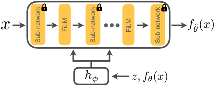
Figure 2: Architecture of RNA. $x$ is the input image, $f_{\theta}$ is the model to be adapted and $f_{\theta}(x)$ the corresponding prediction. To perform adaptation, we freeze the parameters of $f_{\theta}$ and insert several FiLM layers into $f_{\theta}$. We then train $h_{\phi}$ to take in $z$, the adaptation signal, and $f_{\theta}(x)$ to predict the parameters of these FiLM layers. This results in an adapted model $f_{\hat{\theta}}$ and improved predictions, $f_{\hat{\theta}}(x)$.

3.2 Which test-time adaptation signals to use?

While developing adaptation signals is not the main focus of this study and is independent of the RNA method, we need to choose some for experimentation. Existing test-time adaptation signals, or proxies, in the literature include prediction entropy [100], spatial autoencoding [28], and self-supervised tasks like rotation prediction [92], contrastive [60] or clustering [9] objectives. The more aligned the adaptation signal is to the target task, the better the performance on the target task [92, 60]. More importantly, a poor signal can cause the adaptation to fail silently [9, 28]. Figure 3 shows how the original loss on the target task changes as different proxy losses from the literature, i.e. entropy [100], consistency between different middle domains [108, 113] are minimized. In all cases, the proxy loss decreases, however, the improvement in the target loss varies. Thus, successful optimization of existing proxy losses does not necessarily lead to better performance on the target task. In this paper, we adopt a few practical and real-world signals for our study. Furthermore, RNA turns out to be less susceptible to a poor adaptation signal vs TTO (see supplementary Tab. 1). This is because RNA is a neural network trained to use these signals to improve the target task, as opposed to being fixed at being SGD, like in TTO.

3.2.1 Employed test-time adaptation signals

We develop test-time adaptation signals for several geometric and semantic tasks as shown in Fig. 4. Our focus is not on providing an extensive list of adaptation signals, but rather on using practical ones for experimenting with RNA as well as demonstrating the benefits of using signals that are rooted in the known structure of the world and the task in hand. For example, geometric computer vision tasks naturally follow the multi-view geometry constraints, thus making that a proper candidate for approximating the test-time error, and consequently, an informative adaptation signal.

Geometric Tasks. The field of multi-view geometry and its theorems, rooted in the 3D structure of the world, provide a rich source of adaptation signals. We demonstrate our results on the following target tasks: monocular depth estimation, optical-flow estimation, and 3D reconstruction. For all, we first run a standard structure-from-motion (SFM) pipeline [88] to get sparse 3D keypoints. For depth estimation, we employ the z-coordinates of the sparse 3D keypoints i.e., noisy sparse depth, from each image as the adaptation signal. For optical flow, we perform keypoint matching across images. This returns noisy sparse optical flow which we use as the adaptation signal. Lastly, for 3D reconstruction, in addition to the previous two signals, we employ consistency between depth and optical flow predictions as another signal.

Semantic Tasks. For semantic segmentation, we first experiment with using a low number of click annotations for each class, similar to the works on active annotation tools [17, 90, 75]. This gives us sparse segmentation annotations. Likewise, for classification, we use the hierarchical structure of semantic classes, and use coarse labels generated from the WordNet tree [70], similar to [42]. Although these signals (click annotations and coarse labels) are significantly weaker versions of the actual ground truth, thus being cheaper to obtain, it may not be realistic to assume access to them at test-time for certain applications, e.g., real-time ones. Thus, we also show how these can be obtained via $k$-NN retrieval from the training dataset and patch matching using spatial features obtained from a pre-trained self-supervised vision backbone [10] (see Fig. 4).

To perform adaptation with RNA at test-time, we first compute the adaptation signal for the given task as described above. The computed signal and the prediction from the model before adaptation, $f_{\theta}$, are concatenated to form the error feedback. This error feedback is then passed as inputs to $h_{\phi}$ (see Fig. 1). These adaptation signals are practical for real-world use but they are also imperfect i.e., the sparse depth points do not correspond to the ground truth values. Thus, to perform controlled experiments and separate the performance of RNA and adaptation signals, we also provide experiments using ideal adaptation signals, e.g., masked ground truth. In the real world, these ideal signals can come from sensors like LiDAR.

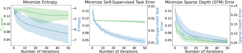
Figure 3: Adaptation using different signals. Not all improvements in proxy loss translates into improving the target task’s performance. We show the results of adapting a pre-trained depth estimation model to a defocus blur corruption by optimizing different adaptation signals: prediction entropy [100], a self-supervised task (sobel edge prediction error [108]), and sparse depth obtained from SFM. The plots show how the $\ell_{1}$ target error with respect to ground-truth depth (green, left axis) changes as the proxy losses (blue, right axis) are optimized (shaded regions represent the 95% confidence intervals across multiple runs of stochastic gradient descent (SGD) with different learning rates). Only adaptation with the sparse depth (SFM) proxy leads to a reduction of the target error. This signifies the importance of employing proper signals in an adaptation framework. Furthermore, we show that RNA is less susceptible to poorer adaptation signal, which results in comparable or improved performance while being significantly faster (see supplementary Table 1).

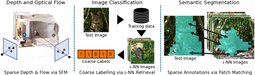
Figure 4: Examples of employed test-time adaptation signals. We use a range of adaptation signals in our experiments. These are practical to obtain and yield better performance compared to other proxies. In the left plot, for depth and optical flow estimation, we use sparse depth and optical flow via SFM. In the middle, for classification, for each test image, we perform $k$-NN retrieval to get $k$ training images. Each of these retrieved image has a one hot label associated with it, thus, combining them gives us a coarse label that we use as our adaptation signal. Finally, for semantic segmentation, after performing $k$-NN as we did for classification, we get a pseudo-labelled segmentation mask for each of these images. The features for each patch in the test image and the retrieved images are matched. The top matches are used as sparse supervision. See Sec. 4.1 for more details.

4 Experiments

We demonstrate that our approach consistently outperforms the baselines for adaptation to different distribution shifts (2D and 3D Common Corruptions [37, 48, 49], cross-datasets), over different tasks (monocular depth, image classification, semantic segmentation, optical flow) and datasets (Taskonomy [114], Replica [91], ImageNet [22], COCO [59], ScanNet [20], Hypersim [84]). The source code can be found on our project page.

4.1 Experimental Setup

We describe our experimental setup, i.e. different adaptation signals, adaptation mechanisms, datasets and baselines, for different tasks. See Tab. 1 for a summary.

Task Adaptation signal Adapted model Training data OOD evaluation data Baselines Depth SFM, masked GT UNet [87], DPT [80] Taskonomy For SFM: Replica, Replica-CC, ScanNet, For masked GT: Taskonomy-CC,-3DCC, Hypersim Pre-adaptation, densification, TENT, TTO-edges, TTO Optical flow Keypoint matching RAFT [94] FlyingChairs, FlyingThings [94] Replica-CC Pre-adaptation 3D reconstruction SFM, keypoint matching, consistency Depth, optical flow models Depth, optical flow data Replica-CC Pre-adaptation, TTO Semantic segmentation Click annotations, patch matching FCN [62] COCO (20 classes from Pascal VOC) For click annotations: COCO-CC, For patch matching: ImageNet-C Pre-adaptation, densification, TENT, TTO Classification Coarse labels (WordNet, DINO $k$-NN) ResNet50 [35], ConvNext [61] ImageNet ImageNet-C, ImageNet-3DCC, ImageNet-V2 Pre-adaptation, DINO $k$-NN, densification, TENT, TTO

Table 1: Overview of the experiments for different target tasks, adaptation methods, and adaptation signals. For each task, we list the adaptation signal (Sec. 3.2) that we use for adaptation. We also list the models that we adapt, and the out-of-distribution (OOD) data used for evaluations and the relevant baselines. When there are different options for adaptation signal, e.g., in the case of depth, the signal is denoted in italics followed by the corresponding OOD dataset. The weights for the semantic segmentation, classification and optical flow models were taken from PyTorch [76].

Baselines. We evaluate the following baselines:

• Pre-Adaptation Baseline: The network $f_{\theta}$ that maps from RGB to the target task, e.g., depth estimation, with no test-time adaptation. We denote this as Baseline for brevity.

• Densification: A network that maps from the given adaptation signal for the target task to the target task, e.g., sparse depth from SFM to dense depth. This is a control baseline and shows what can be learned from the test-time supervision alone, without employing input image information or a designed adaptation architecture. See Sec. 4.3 for a variant which includes the image as an additional input.

• TTO (episodic): We adapt the Baseline model, $f_{\theta}$, to each batch of input images by optimizing the loss computed from the prediction and adaptation signal (see Tab. 1 for the adaptation signal used for each task) at test-time. Its weights are reset to the Baseline model’s after optimizing each batch, similar to [100, 117].

• TTO (online): We continually adapt to a distribution shift defined by a corruption and severity. Test data is assumed to arrive in a stream, and each data point has the same distribution shift, e.g., noise with a fixed standard deviation [100, 92]. The difference with TTO (episodic) is that the model weights are not reset after each iteration. We denote this as TTO for brevity.

• TTO with Entropy supervision (TENT [100]): We adapt the Baseline model trained with log-likelihood loss by optimizing the entropy of the predictions. This is to reveal the effectiveness of entropy as a signal as proposed in [100].

• TTO with Sobel Edges supervision (TTO-Edges): We adapt the Baseline model trained with an additional decoder that predicts a self-supervised task, similar to [92]. We choose to predict Sobel edges as it has been shown to be robust to certain shifts [108]. We optimize the error of the edges predicted by the model and edges extracted from the RGB image to reveal the value of edge error as a supervision.

RNA configurations. At test-time, we first get the predictions of the Baseline model and compute the adaptation signal. The predictions and adaptation signal are then concatenated and passed to $h_{\phi}$ which adapts $f_{\theta}$ to $f_{\hat{\theta}}$. The test images are then passed to $f_{\hat{\theta}}$ to get the final predictions. We evaluate following variants of RNA.

• RNA (frozen $f$): Baseline model weights, $f_{\theta}$, are frozen when training $h_{\phi}$. We call this variant RNA for brevity.

• RNA (jointly trained $f$): In contrast to the frozen $f$ variant, here we train $h_{\phi}$ jointly with the Baseline network. This variant requires longer training.

Figure 5: RNA can achieve similar performance as TTO in a much shorter time. We compare how the $\ell_{1}$ errors of the adaptation mechanisms decrease over wall-clock time (s). The errors are averaged over all episodes (and all corruptions for Replica-CC). RNA only requires a forward pass at test-time, while TTO requires multiple forward and backward passes. On ScanNet and Replica-CC, RNA takes 0.01s, while TTO takes 3s to achieve similar performance. Furthermore, RNA is not trained with test-time shifts unlike TTO, thus, it learned to use the additional supervision to adapt to unseen shifts.

Adaptation signal. As described in Sec. 3.2, we compute a broad range of test-time signals from the following processes. Each case describes a process applied on query image(s) in order to extract a test-time quantity. As mentioned in Sec. 3.2.1, the adaptation signal and prediction from $f_{\theta}$ form the error feedback and the input to $h_{\phi}$.

• Structure-from-motion (SFM): Given a batch of query images, we use COLMAP [88] to run SFM, which returns sparse depth. The percentage of valid pixels, i.e. depth measurements, is about 0.16% on Replica-CC and 0.18% on Replica. For ScanNet we use the pre-computed sparse depth from [85], which has about 0.04% valid pixels. As running SFM on corrupted images results in noisy sparse depth, we train $h_{\phi}$ to be invariant to noise from the adaptation signal [111, 85]. Note that RNA is always trained with clean RGB inputs and only the signal has been corrupted during training.

• Masked ground truth (GT): We apply a random mask to the GT depth of the test image. We fixed the valid pixels to 0.05% of all pixels, i.e. similar sparsity as SFM (see the supplementary for other values). This a control proxy as it enables a better evaluation of the adaptation methods without conflating with the shortcomings of adaptation signals. It is also a scalable way of simulating sparse depth from real-world sensors, e.g., LiDAR, as also done in [101, 65, 44].

• Click annotations: We generate click annotations over random pixels for each class in a given image using GT – simulating an active annotation pipeline. The number of pixels ranges from 3 to 25, i.e. roughly 0.01% of the total pixels, similar to [7, 75, 90, 118, 17].

• Patch matching: To not use GT click annotations, for each test image, we first retrieve its $k$-NN images from the original clean training dataset using DINO features [10]. We then get segmentation masks on these $k$ images. If the training dataset has labels for segmentation we use them directly, otherwise we obtain them from a pretrained network. For each of the $k$ training images and test image, we extract non-overlapping patches. The features for each patch that lie inside the segmentation masks of the $k$ training images are matched to the features of every patch in the test image. These matches are then filtered and used as sparse segmentation annotations. See Fig. 4 for illustration.

• Coarse labels (WordNet): We generate 45 coarse labels from the 1000-way ImageNet labels, i.e. making the labels 22x coarser, using the WordNet tree [70], similar to [41]. See supplementary for more details on the construction and results for other coarse label sets.

• Coarse labels (DINO $k$-NN): For each test image, we retrieve the $k$-NN images from the training dataset using DINO features [10]. Each of these $k$ training images is associated with an ImageNet class, thus, combining $k$ one-hot labels gives us a coarse label.

• Keypoint matching: We perform keypoint matching across images to get sparse optical flow.

Figure 6: Qualitative results of RNA vs the baselines for semantic segmentation on random query images on COCO-CC (left) and depth on images from ScanNet, Taskonomy-3DCC and Replica-CC (right). For semantic segmentation, we use 15 pixel annotations per class. For Taskonomy-3DCC, we use sparse depth with 0.05% valid pixels (30 pixels per image). See Fig. 7 for results on different adaptation signal levels. For ScanNet and Replica-CC, the adaptation signal is sparse depth measurements from SFM [88] with similar sparsity ratios to Taskonomy-3DCC. The predictions with proposed adaptation signals are shown in the last two rows. They are noticeably more accurate compared to the baselines. Comparing TTO and RNA, RNA’s predictions are more accurate for segmentation, and sharper than TTO for depth (see the ellipses) while being significantly faster. See 4.2 and supplementary for more results.

4.2 Adaptation with RNA vs TTO

Here we summarize our observations from adapting with RNA vs TTO. As described, TTO represents the approach of closed-loop adaptation using the adaptation signal but without benefiting from any amortization and learning (the adaptation process is fixed to be standard SGD). These observations hold across different tasks. See Sec. 4.3 for results.

RNA is efficient. As RNA only requires a forward pass at test-time, it is orders of magnitude faster than TTO and is able to attain comparable performance to TTO. In Fig. 5, we compare the runtime of adaption with RNA and TTO for depth prediction. On average, for a given episode, RNA obtains similar performance as TTO in 0.01s, compared to TTO’s 3-5s. Similarly, for dense 3D reconstruction, RNA is able to adapt in 0.008s compared to TTO’s 66s (see Fig. 9). This suggests a successful amortization of the adaptation optimization by RNA.

Furthermore, RNA’s training is also efficient as it only requires training a small model, i.e. 5-20% of the Baseline model’s parameters, depending on the task. Thus, RNA has a fixed overhead, and small added cost at test-time.

RNA’s predictions are sharper than TTO for dense prediction tasks. From the last two rows of Fig. 6, it can be seen that RNA retains fine-grained details. This is a noteworthy point and can be attributed to the fact that RNA benefits from a neural network, thus its inductive biases can be beneficial (and further engineered) for such advantages. This is a general feature that RNA, and more broadly using a learning-based function to amortize adaptation optimization, brings – in contrast to limiting the adaptation process to be SGD, as represented by TTO.

RNA generalizes to unseen shifts. RNA performs better than TTO for low severities (see supplementary for more details). However, as it was not exposed to any corruptions, the performance gap against TTO narrows at high severities as expected, which is exposed to corruptions at test-time.

We hypothesize that the generalization property of RNA is due to the following reasons. Even though $f_{\theta}$ was trained to convergence, it does not achieve exactly 0 error. Thus, when $h_{\phi}$ is trained with a frozen $f_{\theta}$ with the training data, it can still learn to correct the errors of $f_{\theta}$, thus, adapting $f_{\theta}$.

Adaptation Signal SFM Sparse GT Relative Runtime Dataset Replica ScanNet Taskonomy Hypersim Shift CDS CC CDS None CC 3DCC CDS Pre-adaptation Baseline 1.75 6.08 3.30 2.68 5.74 4.75 33.64 1.00 Densification 2.50 4.19 2.35 1.72 1.72 1.72 17.25 1.00 TENT [100] 2.03 6.09 4.03 5.51 5.51 4.48 35.45 15.85 TTO-Edges [92] 1.73 6.14 3.28 2.70 5.69 4.74 33.69 20.98 RNA (frozen $f$) 1.72 4.26 1.77 1.12 1.68 1.49 16.17 1.56 RNA (jointly trained $f$) 1.66 3.41 1.74 1.11 1.50 1.37 17.13 1.56 TTO (Episodic) 1.72 3.31 1.85 1.62 2.99 2.31 17.77 14.85 TTO (Online) 1.82 3.16 1.76 1.13 1.48 1.34 14.17 14.85

Table 2: Quantitative adaptation results on depth estimation. $\ell_{1}$ errors on the depth prediction task. (Lower is better. Multiplied by 100 for readability. The best models within 0.0003 error are shown in bold.) We generate distribution shifts by applying Common Corruptions (CC), 3D Common Corruptions (3DCC) and from performing cross-dataset evaluations (CDS). The results from CC and 3DCC are averaged over all distortions and severity levels on Taskonomy and 3 severity levels on Replica data. The adaptation signal from Taskonomy is masked GT (fixed at 0.05% valid pixels) while that from Replica and ScanNet is sparse depth from SFM. RNA and TTO notably outperform the baselines. RNA successfully matches the performance of TTO while being around 10 times faster. See supplementary for the losses for different corruption types, sparsity levels, and the results of applying RNA to other adaptation signals.

Figure 7: Qualitative adaptation results on semantic segmentation on random query images on COCO-CC. RNA notably improves the prediction quality using error feedback from as few as 3 random pixels.

Figure 8: Quantitative adaptation results on semantic segmentation. Each point shows the mean IOU over 15 corruptions and 5 severities. RNA significantly improves over baselines. Black dashed line shows the mean IOU of the baseline model for clean validation images, and is provided as an upper bound on performance. Numbers in the legend denote averages over all supervision pixel counts. See supplementary for a breakdown.

4.3 Experiments using Various Target Tasks

In this section, we provide a more comprehensive set of evaluations covering various target tasks and adaptation signals. In all cases, RNA is a fixed general framework without being engineered for each task and shows supportive results.

Depth. We demonstrate the results quantitatively in Tab. 2 and Fig. 5 and qualitatively in Fig. 6. In Tab. 2, we compare RNA against all baselines, and over several distribution shifts and different adaptation signals. Our RNA variants outperform the baselines overall. TTO (online) has a better performance than TTO (episodic) as it assumes a smoothly changing distribution shift, and it continuously updates the model weights. RNA (jointly trained $f$) has a better performance among RNA variants. This is reasonable as the target model is not frozen, thus, is less restrictive.

As another baseline, we trained a single model that takes as input a concatenation of the RGB image and sparse supervision, i.e. multi-modal input. However, its average performance on Taskonomy-CC was 42.5% worse than RNA’s (see sup. mat. Sec. 3.2). Among the baselines that do not adapt, densification is the strongest under distribution shift due to corruptions. This is expected as it does not take the RGB image as input, thus, it is not affected by the underlying distribution shift. However, as seen from the qualitative results in Figs. 6, 7, unlike RNA, densification is unable to predict fine-grained details (which quantitative metrics often do not well capture). We also show that the gap between RNA and densification widens with sparser supervision (see sup. mat. Fig. 1), which confirms that RNA is making use of the error feedback signal, to adapt $f$.

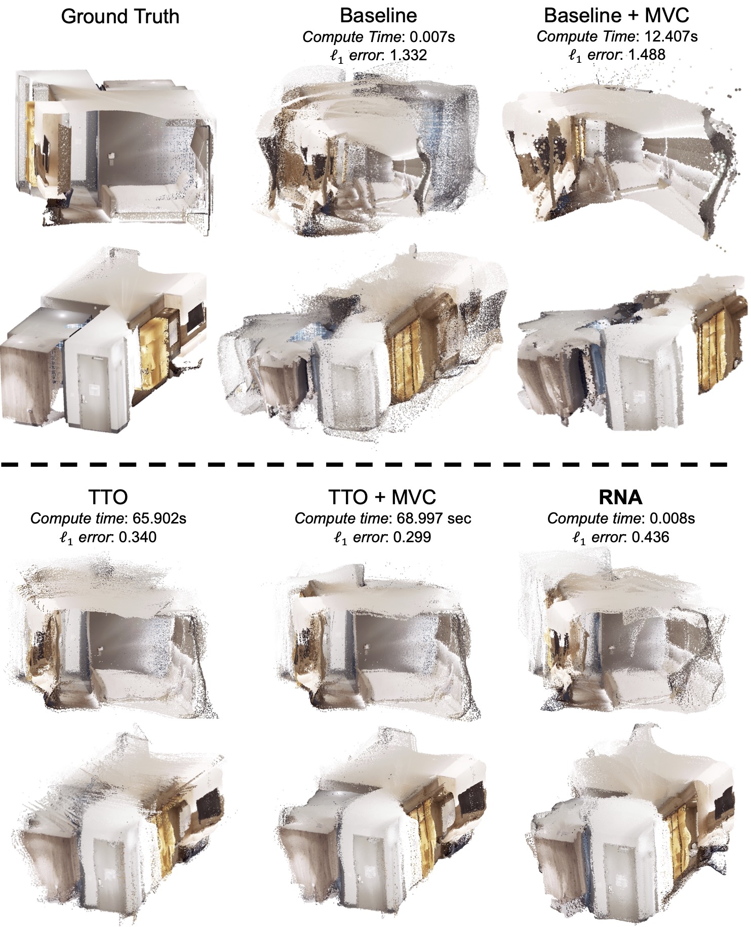
Figure 9: Adaptation results for 3D reconstruction. Using appropriate adaptation signals from multi-view geometry can recover accurate 3D reconstructions. We report the average $\ell_{1}$ error between ground truth 3D coordinates and the estimated ones. The titles above each column refers to the depth model used to get the reconstruction. TTO+MVC corresponds to the predictions after multi-view consistency optimization. It can be seen that RNA and TTO improve the reconstructions over the baselines with RNA being significantly faster. See supplementary Fig. 4 for more results and the corresponding error maps.

Dense 3D Reconstruction. We aim to reconstruct a 3D point cloud of a scene given a sequence of corrupted images. To do so, we make use of multiple adaptation signals from multi-view geometry. First, we compute the noisy sparse depth and optical flow from SFM and use it to adapt the depth and optical flow models. The results from this adaptation can be found in the previous paragraph (for depth) and supplementary (for optical flow). Next, the two models are adapted to make their predictions consistent with each other. This is achieved using multi-view consistency (MVC) constraints, similar to [64]. The predictions from the adapted models are then used in the backprojection to attain a 3D point cloud.

Figure 9 shows the point cloud visualizations on a scene from the Replica dataset. The sequence of input images was corrupted with Gaussian Noise. This results in collapsed depth predictions, thus, the reconstructions are poor (Baseline column) and performing MVC is not helpful (Baseline+MVC). Adapting the depth predictions using TTO and MVC improves the reconstruction notably while RNA achieves a similar performance significantly faster.

Semantic Segmentation. We experiment with click annotations and DINO patch matching as adaptation signals.

Click annotations: In Fig. 8, we show how the IoU changes with the adaptation signal level on COCO-CC. As the Baseline and TENT do not make use of this signal, their IoU is a straight line. RNA clearly outperforms the baselines for all levels of adaptation signal. Figure 7 shows the qualitative results with increasing supervision, and Fig. 6 (left) a comparison against all baselines, demonstrating higher quality predictions with RNA.

DINO patch matching: We perform patch matching on DINO features (described in Sec. 4.1) to get the adaptation signal. As the patch matching process can be computationally expensive, we demonstrate our results on all cat classes in ImageNet and over one noise, blur and digital corruption for 3 levels of severity. We used the predictions of a pre-trained FCN on the clean images as pseudolabels to compute IoU. The mean IoU averaged over these corruptions and severities is 48.98 for the baseline model, 53.45 for TTO. RNA obtains a better IOU of 58.04, thus it can make use of the sparse annotations from DINO patch matching.

Adaptation Signal Dataset Clean IN-C IN-3DCC IN-V2 Rel. Runtime - Pre-adaptation Baseline 23.85 61.66 54.97 37.15 1.00 Entropy TENT 24.67 46.19 47.13 37.07 5.51 Coarse labels (wordnet) Densification 95.50 95.50 95.50 95.50 - TTO (Online) 24.72 40.62 42.90 36.77 5.72 RNA (frozen $f$) 16.72 41.21 40.37 25.53 1.39 Coarse labels (DINO) DINO ($k$-NN) 25.56 52.64 48.24 37.39 - TTO (Online) 24.59 51.59 49.18 36.96 5.72 RNA (frozen $f$) 24.36 54.86 52.29 36.88 1.39

Table 3: Quantitative adaptation results on on ImageNet (IN) classification task. We evaluate on the clean validation set, ImageNet-{C,3DCC,V2}. We report average error (%) for 1000-way classification task over all corruptions and severities. For the coarse labels with WordNet supervision, we use 45-coarse labels. For DINO $k$-NN, we set $k=20$.

Image Classification. We experiment with coarse labels from WordNet and DINO $k$-NN as adaptation signals.

Coarse labels (WordNet): Table 3 shows the results from using 45-coarse labels on ImageNet-{C,3DCC,V2}. This corresponds to 22x coarser supervision compared to the 1000 classes that we are evaluating on. TENT seems to have notable improvements in performance under corruptions for classification, unlike for semantic segmentation and depth. We show that using coarse supervision results in even better performance, about a further 5 pp reduction in error. Furthermore, on uncorrupted data, i.e. clean, and ImageNet-V2 [82], RNA gives roughly 10 pp improvement in performance compared to TTO. Thus, coarse supervision provides a useful signal for adaptation while requiring much less effort than full annotation [106]. See supplementary for results on other coarse sets.

Coarse labels (DINO $k$-NN): We also show results from using coarse sets generated from DINO $k$-NN retrieval. This is shown in the last 3 rows of Tab. 3. Both RNA and TTO use this coarse information to outperform the non-adaptive baselines. However, they do not always outperform TENT, which could be due to the noise in retrieval.

4.4 Ablations and additional results

Task (Arch.) Depth (DPT [80]) Classification (ConvNext [61]) Shift Clean CC Rel. Runtime Clean IN-C Rel. Runtime Pre-adaptation Baseline 2.23 3.76 1.00 18.13 42.95 1.00 TTO (Online) 1.82 2.61 13.85 17.83 41.44 11.04 RNA (frozen $f$) 1.13 1.56 1.01 14.32 38.04 1.07

Table 4: RNA works across different architectures of the main network $f_{\theta}$ such as DPT [80] and ConvNext [61]. Quantitative adaptation results on depth estimation and image classification on Taskonomy and ImageNet datasets, respectively. (Lower is better. $\ell_{1}$ errors for depth estimation are multiplied by 100 for readability.)

Adaptation of other architectures of the main network $f_{\theta}$. Previous results in the paper were from adapting $f_{\theta}$ with a UNet architecture. Here, we study the performance of RNA on other architectures of $f_{\theta}$, namely, the dense prediction transformer (DPT) [80] for depth and ConvNext [61] for image classification. Table 4 shows the results of incorporating RNA to these architectures. In both cases, RNA is able to improve on the error and runtime of TTO. Thus, RNA can be applied to a range of architectures.

Shift Pre-adaptation Baseline Densification TTO RNA CC 0.045 0.023 0.019 0.018

Table 5: Controlling for number of parameters. $\ell_{1}$ errors (multiplied by 100 for readability) on the depth estimation task, evaluated on the Taskonomy test set under a subset of common corruptions. Each method is using the same architecture and number of parameters. The adaptation signal here is masked GT, fixed at 0.05% of valid pixels.

Controlling for different number of parameters. We ran a control experiment where all methods have the same architecture, thus, same number of parameters. The results are in Table 5. RNA still returns the best performance. Thus, its improvement over the baselines is not due to a different architecture or number of parameters but due to its test-time adaptation mechanism.

Method\Shift None Taskonomy-CC Taskonomy-3DCC Hypersim BlendedMVG Pre-adaptation 0.027 0.057 0.048 0.336 3.450 RNA (HyperNetwork-$x$) 0.019 0.041 0.033 0.257 2.587 RNA (FiLM-$x$) 0.019 0.039 0.033 0.279 2.636 RNA (FiLM-$f$) 0.013 0.024 0.020 0.198 2.310

Table 6: Implementations of the controller network $h_{\phi}$ with different architectures. $\ell_{1}$ errors on the depth estimation task under distribution shifts are reported. The adaptation signal here is masked GT, fixed at 0.05% of valid pixels.

Implementations of $h_{\phi}$ with different architectures. We experiment with different architectures for $h_{\phi}$ e.g., HyperNetworks [33], other FiLM variants, or adapting the input instead of the model parameters. Instead of adding FiLM layers to adapt $f_{\theta}$ (denoted as FiLM-$f$), as described in Sec. 3.1, we also experimented with adding FiLM layers to a UNet model that is trained to update the input image $x$ (denoted as FiLM-$x$). For FiLM-$x$, only $x$ is updated and there is no adaptation on $f_{\theta}$. Lastly, as Hypernetworks [33] have been shown to be expressive and suitable for adaptation, we trained a HyperNetwork, in this case an MLP, to predict the weights of a 3-layer convolutional network that updates $x$ (denoted as HyperNetwork-$x$). The results of adaptation with these variants of RNA are shown in Table 6. The FiLM-$f$ variant performed best, thus, we adopted it as our main architecture. See supplementary Sec. 2.2 for further details and a conceptual discussion on the trade-offs of the choices of implementing this closed-loop “control” system, namely those that make stronger model-based assumptions.

5 Approaches for handling distribution shifts

In this section, we provide a unified discussion about the approaches that aim to handle distribution shifts. Figure 10 gives an overview of how these approaches can be characterized. Open-loop systems predict $y$ by only using their inputs without receiving feedback. Training-time robustness methods, image modifications, and multi-modal methods fall into this category. These methods assume the learned model is frozen at the test-time. Thus, they aim to incorporate inductive biases at training time that could be useful against distribution shifts at the test-time. The closed-loop systems, on the other hand, are adaptive as they make use of a live error feedback signal that can be computed at test-time from the model predictions and an adaptation signal.

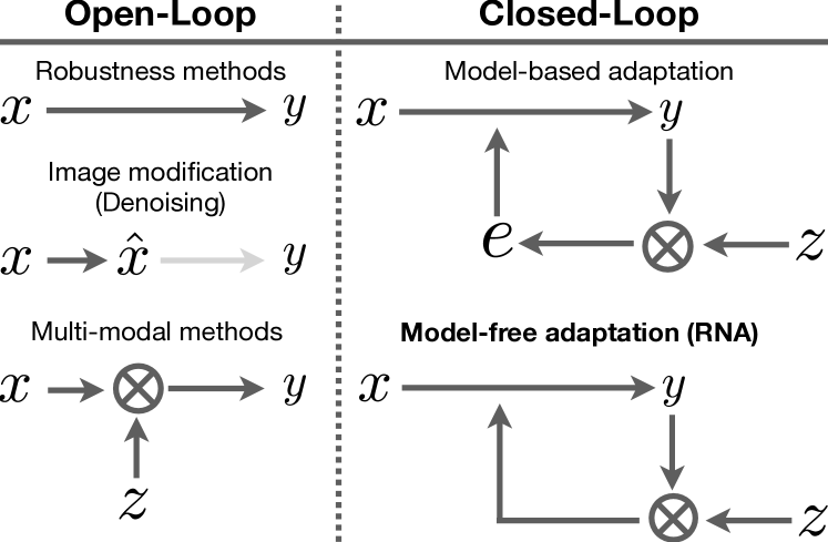
Figure 10: An overview of methods that aim to handle distribution shifts. Left: Open-loop systems predict $y$ by only using their inputs without receiving feedback. The first and popular example of open-loop systems is training-time robustness methods (data augmentation, architectural changes, etc.). The next example is the methods that modify the input $x$, e.g. denoising or style changes, to recover the original image before corruption, independent of $y$. Furthermore, there are multi-modal methods that use an additional input $z$. As the learned model is frozen at test-time, these methods need to anticipate the distribution shift by incorporating inductive biases at training time (See also Fig. 1 of the main paper). Right: In contrast, closed-loop systems make use of its current output, $y$, and an adaptation signal, $z$, to form an error feedback signal that can be used to update its predictions. Thus, they adapt to the shifts as they occur. We can then group closed-loop systems into model-based and model-free methods. The former performs adaptation by estimating the parameters $e$ of specific modeled distribution shift families, while the latter performs adaptation in a data-driven way without explicitly modeling certain distribution shifts. Adaptation can be performed via running an optimization, i.e. TTO via SGD, or via amortization, i.e., training a side controller network to predict TTO updates that minimize the error feedback. Our proposed method, RNA, belongs to the model-free adaptation approach that makes use of amortization for efficiency.

Model-based vs. Model-free: The closed-loop systems can be instantiated as model-based or model-free adaptation methods. The former involves making stronger assumptions and performs adaptation by estimating the parameters of specifically modeled distribution shifts (e.g. blur) using the feedback signal. This is depicted as $e$ in Fig. 10. While this approach often leads to strongly handling the modeled shift and a more interpretable system, conversely it is less likely to generalize to shifts that were not modeled. Our experiments with modeling possible distribution shifts, e.g. the intensity of a noise or blur corruption, did not show significantly better results than the model-free variant, likely for this reason (see supplementary, Sec. 2.2). In contrast, model-free methods do not make explicit assumptions about the distributions shifts and learn to adapt only from the data and based on the error feedback signal. Our proposed method RNA belongs to model-free approaches, and as we showed in the paper, it generalized to a diverse set of unseen distribution shifts.

Observations on RNA vs. RMA [51]. It should be noted that the above observation about model-free vs. model-based approaches and estimating distribution shifts with specific fixed parameters varies based on the domain and problem of interest. For example, in Rapid Motor Adaptation (RMA), Kumar et al.  [51] learned to adapt a policy for legged robots from the data that simulated a fixed set of relevant environment parameters, such as ground friction, terrain height, etc. They showed predicting environment shifts grounded in this fixed set of parameters turns out to be sufficient for a robust adaption generalizable from the simulator to various challenging real-world scenarios. This success did not duplicate for the image recognition problems addressed in this paper despite our attempts. This can be attributed to the lack of a similarly comprehensive simulator and relevant parameter set to sufficiently encapsulate real-world image distortions, as well as possibly the lack of needed inductive biases in the adaption networks.

RNA vs. Denoising. The denoising methods, and in general the methods performing modification in the input image, e.g., domain adaptation methods that aim to map an image in the target domain to the style of the source domain [119], are concerned with reconstructing plausible images without taking the downstream prediction $x\rightarrow y$ into account (shown as gray in Fig. 10). Moreover, it has been shown that imperceptible artifacts in the denoised & modified image could result in degraded predictions [37, 108, 29]. In contrast, RNA performs updates with the goal of reducing the error of the target task.

Multi-modal methods. The closed-loop adaptation methods have schematic similarities to multi-modal learning approaches as they simultaneously use multiple input sources: an RGB input image and an adaptation signal. The main distinction is the adaptation methods implement a particular process toward adapting a network to a shift using an adaptation signal from the environment – as opposed to performing a generic learning using multiple inputs.

Using only the adaptation signal $z$ vs. error feedback as input to $h_{\phi}$. In the case where only the adaptation signal, $z$, is passed as input, it is possible that the side-network is implicitly modelling an error feedback signal. This is because it is trained alongside the main model ($x\rightarrow y$), thus, it sees and learns to correct the main model’s errors during training. We found that having an error feedback signal as input results in better performance on average, thus, we adopted this as our main method.

6 Conclusion and Limitations

We presented RNA, a method for efficient adaptation of neural networks at test-time using a closed-loop formulation. It involves training a side network to use a test-time adaptation signal to adapt a main network. This network acts akin to a “controller” and adapts the main network based on the adaptation signal. We showed that this general and flexible framework can generalize to unseen shifts, and as it only requires a forward pass at test-time, it is orders of magnitude faster than TTO. We evaluated this approach using a diverse set of adaptation signals and target tasks. We briefly discuss the limitations and potential future works:

Different instantiation of RNA and amortization. While we experimented with several RNA variants (see supplementary for details), further investigation toward a stronger instantiation of RNA which can generalize to more shifts and handle more drastic changes, e.g. via building in a more explicit “model” of the shifts and environment (see the discussion about [51]), is important. In general, as the role of the controller network is to amortize the training optimization of the main network, the amortized optimization literature [3] is one apt resource to consult for this purpose.

Hybrid mechanism for activating TTO in RNA. TTO constantly adapts a model to a distribution shift, hence, in theory, it can adapt to any shift despite being comparatively inefficient. To have the best of both worlds, investigating mechanisms for selectively activating TTO within RNA when needed can be useful.

Finding adaptation signals for a given task. While the focus of this study was not on developing new adaption signals, we demonstrated useful ones for several core vision tasks, but there are many more. Finding these signals requires either knowledge of the target task so a meaningful signal can be accordingly engineered or core theoretical works on understanding how a proxy and target objectives can be “aligned” for training.

Acknowledgement: The authors would like to thank Onur Beker. This work was partially supported by the ETH4D and EPFL EssentialTech Centre Humanitarian Action Challenge Grant.

References

- [1] Hassan Akbari, Liangzhe Yuan, Rui Qian, Wei-Hong Chuang, Shih-Fu Chang, Yin Cui, and Boqing Gong. Vatt: Transformers for multimodal self-supervised learning from raw video, audio and text. Advances in Neural Information Processing Systems, 34:24206–24221, 2021.
- [2] Jean-Baptiste Alayrac, Adria Recasens, Rosalia Schneider, Relja Arandjelović, Jason Ramapuram, Jeffrey De Fauw, Lucas Smaira, Sander Dieleman, and Andrew Zisserman. Self-supervised multimodal versatile networks. Advances in Neural Information Processing Systems, 33:25–37, 2020.
- [3] Brandon Amos. Tutorial on amortized optimization for learning to optimize over continuous domains. arXiv preprint arXiv:2202.00665, 2022.
- [4] Marcin Andrychowicz, Misha Denil, Sergio Gomez, Matthew W Hoffman, David Pfau, Tom Schaul, Brendan Shillingford, and Nando De Freitas. Learning to learn by gradient descent by gradient descent. Advances in neural information processing systems, 29, 2016.
- [5] Relja Arandjelovic and Andrew Zisserman. Look, listen and learn. In Proceedings of the IEEE international conference on computer vision, pages 609–617, 2017.
- [6] Roman Bachmann, David Mizrahi, Andrei Atanov, and Amir Zamir. Multimae: Multi-modal multi-task masked autoencoders. In Computer Vision–ECCV 2022: 17th European Conference, Tel Aviv, Israel, October 23–27, 2022, Proceedings, Part XXXVII, pages 348–367. Springer, 2022.
- [7] Amy Bearman, Olga Russakovsky, Vittorio Ferrari, and Li Fei-Fei. What’s the point: Semantic segmentation with point supervision. In European conference on computer vision, pages 549–565. Springer, 2016.
- [8] Srinadh Bhojanapalli, Ayan Chakrabarti, Daniel Glasner, Daliang Li, Thomas Unterthiner, and Andreas Veit. Understanding robustness of transformers for image classification. arXiv preprint arXiv:2103.14586, 2021.
- [9] Malik Boudiaf, Romain Mueller, Ismail Ben Ayed, and Luca Bertinetto. Parameter-free online test-time adaptation. In Proceedings of the IEEE/CVF Conference on Computer Vision and Pattern Recognition, pages 8344–8353, 2022.
- [10] Mathilde Caron, Hugo Touvron, Ishan Misra, Hervé Jégou, Julien Mairal, Piotr Bojanowski, and Armand Joulin. Emerging properties in self-supervised vision transformers. In Proceedings of the IEEE/CVF International Conference on Computer Vision, pages 9650–9660, 2021.
- [11] Joao Carreira, Pulkit Agrawal, Katerina Fragkiadaki, and Jitendra Malik. Human pose estimation with iterative error feedback. In Proceedings of the IEEE conference on computer vision and pattern recognition, pages 4733–4742, 2016.
- [12] Vincent Casser, Soeren Pirk, Reza Mahjourian, and Anelia Angelova. Unsupervised monocular depth and ego-motion learning with structure and semantics. In Proceedings of the IEEE/CVF Conference on Computer Vision and Pattern Recognition Workshops, pages 0–0, 2019.
- [13] Lluis Castrejon, Yusuf Aytar, Carl Vondrick, Hamed Pirsiavash, and Antonio Torralba. Learning aligned cross-modal representations from weakly aligned data. In Proceedings of the IEEE conference on computer vision and pattern recognition, pages 2940–2949, 2016.
- [14] Tianlong Chen, Xiaohan Chen, Wuyang Chen, Howard Heaton, Jialin Liu, Zhangyang Wang, and Wotao Yin. Learning to optimize: A primer and a benchmark. 2021.
- [15] Yun Chen, Bin Yang, Ming Liang, and Raquel Urtasun. Learning joint 2d-3d representations for depth completion. In Proceedings of the IEEE/CVF International Conference on Computer Vision, pages 10023–10032, 2019.
- [16] Yen-Chun Chen, Linjie Li, Licheng Yu, Ahmed El Kholy, Faisal Ahmed, Zhe Gan, Yu Cheng, and Jingjing Liu. Uniter: Universal image-text representation learning. In Computer Vision–ECCV 2020: 16th European Conference, Glasgow, UK, August 23–28, 2020, Proceedings, Part XXX, pages 104–120. Springer, 2020.
- [17] Bowen Cheng, Omkar Parkhi, and Alexander Kirillov. Pointly-supervised instance segmentation. In Proceedings of the IEEE/CVF Conference on Computer Vision and Pattern Recognition, pages 2617–2626, 2022.
- [18] Ilya Chugunov, Yuxuan Zhang, Zhihao Xia, Xuaner Zhang, Jiawen Chen, and Felix Heide. The implicit values of a good hand shake: Handheld multi-frame neural depth refinement. In Proceedings of the IEEE/CVF Conference on Computer Vision and Pattern Recognition, pages 2852–2862, 2022.
- [19] Taco Cohen and Max Welling. Group equivariant convolutional networks. In International conference on machine learning, pages 2990–2999. PMLR, 2016.
- [20] Angela Dai, Angel X Chang, Manolis Savva, Maciej Halber, Thomas Funkhouser, and Matthias Nießner. Scannet: Richly-annotated 3d reconstructions of indoor scenes. In Proceedings of the IEEE Conference on Computer Vision and Pattern Recognition, pages 5828–5839, 2017.
- [21] Marc Deisenroth and Carl E Rasmussen. Pilco: A model-based and data-efficient approach to policy search. In Proceedings of the 28th International Conference on machine learning (ICML-11), pages 465–472, 2011.
- [22] Jia Deng, Wei Dong, Richard Socher, Li-Jia Li, Kai Li, and Li Fei-Fei. Imagenet: A large-scale hierarchical image database. In 2009 IEEE Conference on Computer Vision and Pattern Recognition, pages 248–255. Ieee, 2009.
- [23] Samuel Dodge and Lina Karam. A study and comparison of human and deep learning recognition performance under visual distortions. In 2017 26th International Conference on Computer Communication and Networks (ICCCN), pages 1–7. IEEE, 2017.
- [24] Vincent Dumoulin, Ethan Perez, Nathan Schucher, Florian Strub, Harm de Vries, Aaron Courville, and Yoshua Bengio. Feature-wise transformations. Distill, 2018. https://distill.pub/2018/feature-wise-transformations.
- [25] Vincent Dumoulin, Jonathon Shlens, and Manjunath Kudlur. A learned representation for artistic style. arXiv preprint arXiv:1610.07629, 2016.
- [26] Ainaz Eftekhar, Alexander Sax, Jitendra Malik, and Amir Zamir. Omnidata: A scalable pipeline for making multi-task mid-level vision datasets from 3d scans. In Proceedings of the IEEE/CVF International Conference on Computer Vision, pages 10786–10796, 2021.
- [27] Chelsea Finn, Pieter Abbeel, and Sergey Levine. Model-agnostic meta-learning for fast adaptation of deep networks. In International conference on machine learning, pages 1126–1135. PMLR, 2017.
- [28] Yossi Gandelsman, Yu Sun, Xinlei Chen, and Alexei A Efros. Test-time training with masked autoencoders. arXiv preprint arXiv:2209.07522, 2022.
- [29] Jin Gao, Jialing Zhang, Xihui Liu, Trevor Darrell, Evan Shelhamer, and Dequan Wang. Back to the source: Diffusion-driven test-time adaptation. arXiv preprint arXiv:2207.03442, 2022.
- [30] Robert Geirhos, Jörn-Henrik Jacobsen, Claudio Michaelis, Richard Zemel, Wieland Brendel, Matthias Bethge, and Felix A Wichmann. Shortcut learning in deep neural networks. arXiv preprint arXiv:2004.07780, 2020.
- [31] Golnaz Ghiasi, Honglak Lee, Manjunath Kudlur, Vincent Dumoulin, and Jonathon Shlens. Exploring the structure of a real-time, arbitrary neural artistic stylization network. arXiv preprint arXiv:1705.06830, 2017.
- [32] Rohit Girdhar, Mannat Singh, Nikhila Ravi, Laurens van der Maaten, Armand Joulin, and Ishan Misra. Omnivore: A single model for many visual modalities. In Proceedings of the IEEE/CVF Conference on Computer Vision and Pattern Recognition, pages 16102–16112, 2022.
- [33] David Ha, Andrew Dai, and Quoc V Le. Hypernetworks. arXiv preprint arXiv:1609.09106, 2016.
- [34] Kaiming He, Xinlei Chen, Saining Xie, Yanghao Li, Piotr Dollár, and Ross Girshick. Masked autoencoders are scalable vision learners. In Proceedings of the IEEE/CVF Conference on Computer Vision and Pattern Recognition, pages 16000–16009, 2022.
- [35] Kaiming He, Xiangyu Zhang, Shaoqing Ren, and Jian Sun. Deep residual learning for image recognition. In Proceedings of the IEEE Conference on Computer Vision and Pattern Recognition, pages 770–778, 2016.
- [36] Dan Hendrycks, Steven Basart, Norman Mu, Saurav Kadavath, Frank Wang, Evan Dorundo, Rahul Desai, Tyler Zhu, Samyak Parajuli, Mike Guo, et al. The many faces of robustness: A critical analysis of out-of-distribution generalization. In Proceedings of the IEEE/CVF International Conference on Computer Vision, pages 8340–8349, 2021.
- [37] Dan Hendrycks and Thomas Dietterich. Benchmarking neural network robustness to common corruptions and perturbations. arXiv preprint arXiv:1903.12261, 2019.
- [38] Dan Hendrycks, Kimin Lee, and Mantas Mazeika. Using pre-training can improve model robustness and uncertainty. In International Conference on Machine Learning, pages 2712–2721. PMLR, 2019.
- [39] Dan Hendrycks, Norman Mu, Ekin D Cubuk, Barret Zoph, Justin Gilmer, and Balaji Lakshminarayanan. Augmix: A simple data processing method to improve robustness and uncertainty. arXiv preprint arXiv:1912.02781, 2019.
- [40] Xun Huang and Serge Belongie. Arbitrary style transfer in real-time with adaptive instance normalization. In Proceedings of the IEEE International Conference on Computer Vision, pages 1501–1510, 2017.
- [41] Minyoung Huh, Pulkit Agrawal, and Alexei A. Efros. What makes imagenet good for transfer learning?, 2016.
- [42] Minyoung Huh, Pulkit Agrawal, and Alexei A Efros. What makes imagenet good for transfer learning? arXiv preprint arXiv:1608.08614, 2016.
- [43] Saachi Jain, Dimitris Tsipras, and Aleksander Madry. Combining diverse feature priors. In International Conference on Machine Learning, pages 9802–9832. PMLR, 2022.
- [44] Maximilian Jaritz, Raoul De Charette, Emilie Wirbel, Xavier Perrotton, and Fawzi Nashashibi. Sparse and dense data with cnns: Depth completion and semantic segmentation. In 2018 International Conference on 3D Vision (3DV), pages 52–60. IEEE, 2018.
- [45] Xiang Jiang, Mohammad Havaei, Farshid Varno, Gabriel Chartrand, Nicolas Chapados, and Stan Matwin. Learning to learn with conditional class dependencies. In international conference on learning representations, 2019.
- [46] Jason Jo and Yoshua Bengio. Measuring the tendency of cnns to learn surface statistical regularities. arXiv preprint arXiv:1711.11561, 2017.
- [47] Di Kang, Debarun Dhar, and Antoni Chan. Incorporating side information by adaptive convolution. Advances in Neural Information Processing Systems, 30, 2017.
- [48] Oğuzhan Fatih Kar, Teresa Yeo, Andrei Atanov, and Amir Zamir. 3d common corruptions and data augmentation. In Proceedings of the IEEE/CVF Conference on Computer Vision and Pattern Recognition, pages 18963–18974, 2022.
- [49] Oğuzhan Fatih Kar, Teresa Yeo, and Amir Zamir. 3d common corruptions for object recognition. In ICML 2022 Shift Happens Workshop, 2022.
- [50] Johannes Kopf, Xuejian Rong, and Jia-Bin Huang. Robust consistent video depth estimation. In Proceedings of the IEEE/CVF Conference on Computer Vision and Pattern Recognition, pages 1611–1621, 2021.
- [51] Ashish Kumar, Zipeng Fu, Deepak Pathak, and Jitendra Malik. Rma: Rapid motor adaptation for legged robots. arXiv preprint arXiv:2107.04034, 2021.
- [52] Yevhen Kuznietsov, Marc Proesmans, and Luc Van Gool. Comoda: Continuous monocular depth adaptation using past experiences. In Proceedings of the IEEE/CVF Winter Conference on Applications of Computer Vision, pages 2907–2917, 2021.
- [53] Balaji Lakshminarayanan, Alexander Pritzel, and Charles Blundell. Simple and scalable predictive uncertainty estimation using deep ensembles. In Advances in Neural Information Processing Systems, pages 6402–6413, 2017.
- [54] Ke Li and Jitendra Malik. Learning to optimize. arXiv preprint arXiv:1606.01885, 2016.
- [55] Liunian Harold Li, Mark Yatskar, Da Yin, Cho-Jui Hsieh, and Kai-Wei Chang. Visualbert: A simple and performant baseline for vision and language. arXiv preprint arXiv:1908.03557, 2019.
- [56] Jian Liang, Dapeng Hu, and Jiashi Feng. Do we really need to access the source data? source hypothesis transfer for unsupervised domain adaptation. In International Conference on Machine Learning, pages 6028–6039. PMLR, 2020.
- [57] Timothy P Lillicrap, Jonathan J Hunt, Alexander Pritzel, Nicolas Heess, Tom Erez, Yuval Tassa, David Silver, and Daan Wierstra. Continuous control with deep reinforcement learning. arXiv preprint arXiv:1509.02971, 2015.
- [58] Di Lin, Jifeng Dai, Jiaya Jia, Kaiming He, and Jian Sun. Scribblesup: Scribble-supervised convolutional networks for semantic segmentation. In Proceedings of the IEEE conference on computer vision and pattern recognition, pages 3159–3167, 2016.
- [59] Tsung-Yi Lin, Michael Maire, Serge Belongie, James Hays, Pietro Perona, Deva Ramanan, Piotr Dollár, and C Lawrence Zitnick. Microsoft coco: Common objects in context. In European Conference on Computer Vision, pages 740–755. Springer, 2014.
- [60] Yuejiang Liu, Parth Kothari, Bastien van Delft, Baptiste Bellot-Gurlet, Taylor Mordan, and Alexandre Alahi. Ttt++: When does self-supervised test-time training fail or thrive? Advances in Neural Information Processing Systems, 34:21808–21820, 2021.
- [61] Zhuang Liu, Hanzi Mao, Chao-Yuan Wu, Christoph Feichtenhofer, Trevor Darrell, and Saining Xie. A convnet for the 2020s. In Proceedings of the IEEE/CVF Conference on Computer Vision and Pattern Recognition, pages 11976–11986, 2022.
- [62] Jonathan Long, Evan Shelhamer, and Trevor Darrell. Fully convolutional networks for semantic segmentation. In Proceedings of the IEEE Conference on Computer Vision and Pattern Recognition, pages 3431–3440, 2015.
- [63] Raphael Gontijo Lopes, Dong Yin, Ben Poole, Justin Gilmer, and Ekin D Cubuk. Improving robustness without sacrificing accuracy with patch gaussian augmentation. arXiv preprint arXiv:1906.02611, 2019.
- [64] Xuan Luo, Jia-Bin Huang, Richard Szeliski, Kevin Matzen, and Johannes Kopf. Consistent video depth estimation. ACM Transactions on Graphics (ToG), 39(4):71–1, 2020.
- [65] Fangchang Ma and Sertac Karaman. Sparse-to-dense: Depth prediction from sparse depth samples and a single image. In 2018 IEEE international conference on robotics and automation (ICRA), pages 4796–4803. IEEE, 2018.
- [66] Wei-Chiu Ma, Shenlong Wang, Jiayuan Gu, Sivabalan Manivasagam, Antonio Torralba, and Raquel Urtasun. Deep feedback inverse problem solver. In Computer Vision–ECCV 2020: 16th European Conference, Glasgow, UK, August 23–28, 2020, Proceedings, Part V 16, pages 229–246. Springer, 2020.
- [67] Aleksander Madry, Aleksandar Makelov, Ludwig Schmidt, Dimitris Tsipras, and Adrian Vladu. Towards deep learning models resistant to adversarial attacks. arXiv preprint arXiv:1706.06083, 2017.
- [68] Xiaofeng Mao, Gege Qi, Yuefeng Chen, Xiaodan Li, Ranjie Duan, Shaokai Ye, Yuan He, and Hui Xue. Towards robust vision transformer. In Proceedings of the IEEE/CVF Conference on Computer Vision and Pattern Recognition, pages 12042–12051, 2022.
- [69] Joe Marino, Yisong Yue, and Stephan Mandt. Iterative amortized inference. In International Conference on Machine Learning, pages 3403–3412. PMLR, 2018.
- [70] George A. Miller. WordNet: A lexical database for English. In Human Language Technology: Proceedings of a Workshop held at Plainsboro, New Jersey, March 8-11, 1994, 1994.
- [71] Shuaicheng Niu, Jiaxiang Wu, Yifan Zhang, Zhiquan Wen, Yaofo Chen, Peilin Zhao, and Mingkui Tan. Towards stable test-time adaptation in dynamic wild world. arXiv preprint arXiv:2302.12400, 2023.
- [72] Boris Oreshkin, Pau Rodríguez López, and Alexandre Lacoste. Tadam: Task dependent adaptive metric for improved few-shot learning. Advances in neural information processing systems, 31, 2018.
- [73] Yaniv Ovadia, Emily Fertig, Jie Ren, Zachary Nado, David Sculley, Sebastian Nowozin, Joshua Dillon, Balaji Lakshminarayanan, and Jasper Snoek. Can you trust your model’s uncertainty? evaluating predictive uncertainty under dataset shift. In Advances in Neural Information Processing Systems, pages 13991–14002, 2019.
- [74] Matteo Pagliardini, Martin Jaggi, François Fleuret, and Sai Praneeth Karimireddy. Agree to disagree: Diversity through disagreement for better transferability. arXiv preprint arXiv:2202.04414, 2022.
- [75] Dim P Papadopoulos, Jasper RR Uijlings, Frank Keller, and Vittorio Ferrari. Extreme clicking for efficient object annotation. In Proceedings of the IEEE international conference on computer vision, pages 4930–4939, 2017.
- [76] Adam Paszke, Sam Gross, Francisco Massa, Adam Lerer, James Bradbury, Gregory Chanan, Trevor Killeen, Zeming Lin, Natalia Gimelshein, Luca Antiga, et al. Pytorch: An imperative style, high-performance deep learning library. In Advances in Neural Information Processing Systems, pages 8024–8035, 2019.
- [77] Ethan Perez, Florian Strub, Harm De Vries, Vincent Dumoulin, and Aaron Courville. Film: Visual reasoning with a general conditioning layer. In Proceedings of the AAAI Conference on Artificial Intelligence, volume 32, 2018.
- [78] Alec Radford, Jong Wook Kim, Chris Hallacy, Aditya Ramesh, Gabriel Goh, Sandhini Agarwal, Girish Sastry, Amanda Askell, Pamela Mishkin, Jack Clark, et al. Learning transferable visual models from natural language supervision. In International conference on machine learning, pages 8748–8763. PMLR, 2021.
- [79] Alexandre Rame and Matthieu Cord. Dice: Diversity in deep ensembles via conditional redundancy adversarial estimation. arXiv preprint arXiv:2101.05544, 2021.
- [80] René Ranftl, Alexey Bochkovskiy, and Vladlen Koltun. Vision transformers for dense prediction. In Proceedings of the IEEE/CVF International Conference on Computer Vision, pages 12179–12188, 2021.
- [81] René Ranftl, Katrin Lasinger, David Hafner, Konrad Schindler, and Vladlen Koltun. Towards robust monocular depth estimation: Mixing datasets for zero-shot cross-dataset transfer. IEEE Transactions on Pattern Analysis and Machine Intelligence, 44(3), 2022.
- [82] Benjamin Recht, Rebecca Roelofs, Ludwig Schmidt, and Vaishaal Shankar. Do imagenet classifiers generalize to imagenet? In International Conference on Machine Learning, pages 5389–5400. PMLR, 2019.
- [83] James Requeima, Jonathan Gordon, John Bronskill, Sebastian Nowozin, and Richard E Turner. Fast and flexible multi-task classification using conditional neural adaptive processes. Advances in Neural Information Processing Systems, 32, 2019.
- [84] Mike Roberts, Jason Ramapuram, Anurag Ranjan, Atulit Kumar, Miguel Angel Bautista, Nathan Paczan, Russ Webb, and Joshua M Susskind. Hypersim: A photorealistic synthetic dataset for holistic indoor scene understanding. In Proceedings of the IEEE/CVF International Conference on Computer Vision, pages 10912–10922, 2021.
- [85] Barbara Roessle, Jonathan T Barron, Ben Mildenhall, Pratul P Srinivasan, and Matthias Nießner. Dense depth priors for neural radiance fields from sparse input views. In Proceedings of the IEEE/CVF Conference on Computer Vision and Pattern Recognition, pages 12892–12901, 2022.
- [86] Robin Rombach, Andreas Blattmann, Dominik Lorenz, Patrick Esser, and Björn Ommer. High-resolution image synthesis with latent diffusion models. In Proceedings of the IEEE/CVF Conference on Computer Vision and Pattern Recognition, pages 10684–10695, 2022.
- [87] Olaf Ronneberger, Philipp Fischer, and Thomas Brox. U-net: Convolutional networks for biomedical image segmentation. In International Conference on Medical Image Computing and Computer-assisted Intervention, pages 234–241. Springer, 2015.
- [88] Johannes Lutz Schönberger and Jan-Michael Frahm. Structure-from-motion revisited. In Conference on Computer Vision and Pattern Recognition (CVPR), 2016.
- [89] Rulin Shao, Zhouxing Shi, Jinfeng Yi, Pin-Yu Chen, and Cho-Jui Hsieh. On the adversarial robustness of visual transformers. arXiv preprint arXiv:2103.15670, 2021.
- [90] Gyungin Shin, Weidi Xie, and Samuel Albanie. All you need are a few pixels: semantic segmentation with pixelpick. In Proceedings of the IEEE/CVF International Conference on Computer Vision, pages 1687–1697, 2021.
- [91] Julian Straub, Thomas Whelan, Lingni Ma, Yufan Chen, Erik Wijmans, Simon Green, Jakob J. Engel, Raul Mur-Artal, Carl Ren, Shobhit Verma, Anton Clarkson, Mingfei Yan, Brian Budge, Yajie Yan, Xiaqing Pan, June Yon, Yuyang Zou, Kimberly Leon, Nigel Carter, Jesus Briales, Tyler Gillingham, Elias Mueggler, Luis Pesqueira, Manolis Savva, Dhruv Batra, Hauke M. Strasdat, Renzo De Nardi, Michael Goesele, Steven Lovegrove, and Richard Newcombe. The Replica dataset: A digital replica of indoor spaces. arXiv preprint arXiv:1906.05797, 2019.
- [92] Yu Sun, Xiaolong Wang, Zhuang Liu, John Miller, Alexei Efros, and Moritz Hardt. Test-time training with self-supervision for generalization under distribution shifts. In International conference on machine learning, pages 9229–9248. PMLR, 2020.
- [93] Hao Tan and Mohit Bansal. Lxmert: Learning cross-modality encoder representations from transformers. arXiv preprint arXiv:1908.07490, 2019.
- [94] Zachary Teed and Jia Deng. Raft: Recurrent all-pairs field transforms for optical flow. In European conference on computer vision, pages 402–419. Springer, 2020.
- [95] Eleni Triantafillou, Hugo Larochelle, Richard Zemel, and Vincent Dumoulin. Learning a universal template for few-shot dataset generalization. In International Conference on Machine Learning, pages 10424–10433. PMLR, 2021.
- [96] Eleni Triantafillou, Tyler Zhu, Vincent Dumoulin, Pascal Lamblin, Utku Evci, Kelvin Xu, Ross Goroshin, Carles Gelada, Kevin Swersky, Pierre-Antoine Manzagol, et al. Meta-dataset: A dataset of datasets for learning to learn from few examples. arXiv preprint arXiv:1903.03096, 2019.
- [97] Ashish Vaswani, Noam Shazeer, Niki Parmar, Jakob Uszkoreit, Llion Jones, Aidan N Gomez, Łukasz Kaiser, and Illia Polosukhin. Attention is all you need. Advances in neural information processing systems, 30, 2017.
- [98] Yannick Verdié, Jifei Song, Barnabé Mas, Benjamin Busam, Aleš Leonardis, and Steven McDonagh. Cromo: Cross-modal learning for monocular depth estimation. In 2022 IEEE/CVF Conference on Computer Vision and Pattern Recognition (CVPR), pages 3927–3937. IEEE, 2022.
- [99] Oriol Vinyals, Charles Blundell, Timothy Lillicrap, Daan Wierstra, et al. Matching networks for one shot learning. Advances in neural information processing systems, 29, 2016.
- [100] Dequan Wang, Evan Shelhamer, Shaoteng Liu, Bruno Olshausen, and Trevor Darrell. Tent: Fully test-time adaptation by entropy minimization. In International Conference on Learning Representations, 2020.
- [101] Tsun-Hsuan Wang, Fu-En Wang, Juan-Ting Lin, Yi-Hsuan Tsai, Wei-Chen Chiu, and Min Sun. Plug-and-play: Improve depth prediction via sparse data propagation. In 2019 International Conference on Robotics and Automation (ICRA), pages 5880–5886. IEEE, 2019.
- [102] Jamie Watson, Oisin Mac Aodha, Victor Prisacariu, Gabriel Brostow, and Michael Firman. The temporal opportunist: Self-supervised multi-frame monocular depth. In Proceedings of the IEEE/CVF Conference on Computer Vision and Pattern Recognition, pages 1164–1174, 2021.
- [103] Olga Wichrowska, Niru Maheswaranathan, Matthew W Hoffman, Sergio Gomez Colmenarejo, Misha Denil, Nando Freitas, and Jascha Sohl-Dickstein. Learned optimizers that scale and generalize. In International conference on machine learning, pages 3751–3760. PMLR, 2017.
- [104] Qizhe Xie, Minh-Thang Luong, Eduard Hovy, and Quoc V Le. Self-training with noisy student improves imagenet classification. In Proceedings of the IEEE/CVF Conference on Computer Vision and Pattern Recognition, pages 10687–10698, 2020.
- [105] Sang Michael Xie, Ananya Kumar, Robbie Jones, Fereshte Khani, Tengyu Ma, and Percy Liang. In-n-out: Pre-training and self-training using auxiliary information for out-of-distribution robustness. arXiv preprint arXiv:2012.04550, 2020.
- [106] Yuanhong Xu, Qi Qian, Hao Li, Rong Jin, and Juhua Hu. Weakly supervised representation learning with coarse labels. In Proceedings of the IEEE/CVF International Conference on Computer Vision, pages 10593–10601, 2021.
- [107] Yanchao Yang, Alex Wong, and Stefano Soatto. Dense depth posterior (ddp) from single image and sparse range. In Proceedings of the IEEE/CVF Conference on Computer Vision and Pattern Recognition, pages 3353–3362, 2019.
- [108] Teresa Yeo, Oğuzhan Fatih Kar, and Amir Zamir. Robustness via cross-domain ensembles. In Proceedings of the IEEE/CVF International Conference on Computer Vision (ICCV), pages 12189–12199, October 2021.
- [109] Chenyu Yi, Siyuan Yang, Yufei Wang, Haoliang Li, Yap-Peng Tan, and Alex C Kot. Temporal coherent test-time optimization for robust video classification. arXiv preprint arXiv:2302.14309, 2023.
- [110] Dong Yin, Raphael Gontijo Lopes, Jon Shlens, Ekin Dogus Cubuk, and Justin Gilmer. A fourier perspective on model robustness in computer vision. In Advances in Neural Information Processing Systems, pages 13276–13286, 2019.
- [111] Wei Yin, Jianming Zhang, Oliver Wang, Simon Niklaus, Simon Chen, and Chunhua Shen. Towards domain-agnostic depth completion. arXiv preprint arXiv:2207.14466, 2022.
- [112] Sangdoo Yun, Dongyoon Han, Seong Joon Oh, Sanghyuk Chun, Junsuk Choe, and Youngjoon Yoo. Cutmix: Regularization strategy to train strong classifiers with localizable features. In Proceedings of the IEEE/CVF International Conference on Computer Vision, pages 6023–6032, 2019.
- [113] Amir Zamir, Alexander Sax, Teresa Yeo, Oğuzhan Kar, Nikhil Cheerla, Rohan Suri, Zhangjie Cao, Jitendra Malik, and Leonidas Guibas. Robust learning through cross-task consistency. arXiv preprint arXiv:2006.04096, 2020.
- [114] Amir R Zamir, Alexander Sax, William Shen, Leonidas J Guibas, Jitendra Malik, and Silvio Savarese. Taskonomy: Disentangling task transfer learning. In Proceedings of the IEEE Conference on Computer Vision and Pattern Recognition, pages 3712–3722, 2018.
- [115] Amir R Zamir, Te-Lin Wu, Lin Sun, William B Shen, Bertram E Shi, Jitendra Malik, and Silvio Savarese. Feedback networks. In Proceedings of the IEEE conference on computer vision and pattern recognition, pages 1308–1317, 2017.
- [116] Hongyi Zhang, Moustapha Cisse, Yann N Dauphin, and David Lopez-Paz. mixup: Beyond empirical risk minimization. arXiv preprint arXiv:1710.09412, 2017.
- [117] Marvin Zhang, Sergey Levine, and Chelsea Finn. Memo: Test time robustness via adaptation and augmentation. arXiv preprint arXiv:2110.09506, 2021.
- [118] Shuaifeng Zhi, Tristan Laidlow, Stefan Leutenegger, and Andrew J Davison. In-place scene labelling and understanding with implicit scene representation. In Proceedings of the IEEE/CVF International Conference on Computer Vision, pages 15838–15847, 2021.
- [119] Jun-Yan Zhu, Taesung Park, Phillip Isola, and Alexei A Efros. Unpaired image-to-image translation using cycle-consistent adversarial networks. In Proceedings of the IEEE International Conference on Computer Vision, pages 2223–2232, 2017.
- [120] Luisa Zintgraf, Kyriacos Shiarli, Vitaly Kurin, Katja Hofmann, and Shimon Whiteson. Fast context adaptation via meta-learning. In International Conference on Machine Learning, pages 7693–7702. PMLR, 2019.