Noise propagation in hybrid tensor networks

Abstract

The hybrid tensor network (HTN) method is a general framework allowing for the construction of an effective wavefunction with the combination of classical tensors and quantum tensors, i.e., amplitudes of quantum states. In particular, hybrid tree tensor networks (HTTNs) are very useful for simulating larger systems beyond the available size of the quantum hardware. However, while the realistic quantum states in NISQ hardware are highly likely to be noisy, this framework is formulated for pure states. In this work, as well as discussing the relevant methods, i.e., Deep VQE and entanglement forging under the framework of HTTNs, we investigate the noisy HTN states by introducing the expansion operator for providing the description of the expansion of the size of simulated quantum systems and the noise propagation. This framework enables the general tree HTN states to be explicitly represented and their physicality to be discussed. We also show that the expectation value of a measured observable exponentially vanishes with the number of contracted quantum tensors. Our work will lead to providing the noise-resilient construction of HTN states.

I introduction

Noisy intermediate-scale quantum (NISQ) computers are expected to have many applications ranging from quantum computational chemistry [1, 2] to machine learning [3, 4] and even quantum sensing [5, 6]. However, despite the potential significant advantages of NISQ devices [7, 8, 9], many obstacles need to be overcome for practical applications. One of the significant problems is the scalability of quantum computers: the largest number of integrated qubits is restricted to the order of $10^{2}$ [10, 11], and we need technical leaps to scale quantum computers beyond.

Considering the current situation of scalability of NISQ computers, a couple of methods are being developed to effectively enlarge the simulated quantum systems, e.g., entangling forging [12, 13, 14], Deep variational quantum eigensolver (DeepVQE) [15, 16, 17], and hybrid tensor networks (HTN) [18, 19, 20]. Additional operations on quantum computers and classical post-processing of measurement outcomes allow us to virtually emulate the effect of quantum entanglement between subsystems when we compute expectation values of observables. Since many NISQ algorithms rely on the measurement of observables, for example, the variational quantum eigensolver (VQE) [21, 1, 2], optimizes the energy of molecules, i.e., the expectation values of the Hamiltonian, these techniques are quite useful in NISQ applications.

In particular, the HTN framework is a quite general framework that comprehensively discusses the hybridization of quantum tensors and classical tensors [18]. While classical tensors are the same as conventional tensors, quantum tensors refer to amplitudes of quantum states, which have two types of indices: classical index and quantum index. Suppose an example of quantum tensor $\ket{\psi^{i}}=\sum_{i_{1},i_{2},...,i_{k}}\psi_{i_{1},i_{2},...i_{k}}^{i}\ket{i_{1},i_{2},...i_{k}}$, where $\ket{i_{k}}$ ($~{}i_{k}\in\{0,1\}~{}\forall k$) indicates qubit states; the upper index $i$ indicate the classical tensors contracted in a similar vein to a conventional classical tensor with lower indices being quantum indices, which is contracted through quantum measurements because it is relevant to qubits. It has also been pointed out that hybrid tree tensor networks (HTTNs) are significantly useful for simulating larger quantum systems.

While the above frameworks for simulating larger quantum systems are appealing for small-scale NISQ devices, another massive problem in NISQ devices is inevitable noise effects due to unwanted system interactions with the environment [8, 7]. We remark that those methods for expanding the simulated quantum systems have been analyzed only for pure states under the assumption that noise effects are negligible [18, 15, 12]. However, such a strong assumption does not reflect the reality of the current situation in which NISQ devices suffer from a significant amount of computation errors.

In the present paper, we try to bridge the gap between the theoretical framework and the actual experiments. To do so, we first show that Deep VQE and entangling forging can be discussed with the language of HTN, especially HTTNs. Next, we introduce the expansion operator to consistently describe the propagation of noise and expansion of the simulated quantum system in HTN states. Note that we detail the form of the expansion operator depending on the type of tensor contractions. This argument allows us to represent the explicit form of general multiple-layer tree HTN states and discuss their physicality, i.e., whether the noisy HTN states $\tilde{\rho}_{\rm HT}$ satisfies the positivity $\tilde{\rho}_{\rm HT}\geq 0$. In addition, we reveal that the computation results from noisy tree tensor states become exponentially small with the number of contracted quantum tensors, which indicates that adjustments of the number of quantum tensors and classical tensors are required in the realistic experimental setup.

The remainder of this paper is organized as follows. In Sec. II, we review the framework of HTN, highlighting the importance of tree tensor networks and classifying the contraction rules of quantum tensors. In Sec. III, we reformulate the Deep VQE and entanglement-forging methods under the framework of HTTNs. In Sec. IV, we study the explicit form of the expansion operator in accordance with the contraction rules and discuss the physicality of the HTN states. In Sec. V, we discuss the exponential decay of the observable with the number of quantum tensors. Finally, we conclude this paper with discussions and conclusions.

II Hybrid Tensor Networks

Classical tensor network (TN) methods [22, 23, 24, 25, 26] try to efficiently describe quantum states of interest with a much smaller subset of the entire Hilbert space on the basis of physical observation. For example, the matrix product state (MPS) [24] ansatz represents the state as

$$\ket{\psi_{\rm MPS}}=\sum_{j_{1},j_{2},...,j_{M}}\mathrm{Tr}[A_{1}^{j_{1}}A_{2}^{j_{2}}...A_{M}^{j_{M}}]\ket{j_{1},j_{2},...,j_{M}},$$ (1)

where $j_{k}$ takes $0$ or $1$ in the case of qubit systems, and $A_{1}$ and $A_{M}$ are rank-2 tensors with $A_{k}$ being rank-3 tensors. This ansatz construction allows us to compress the number of parameters representing the state to $O(M\kappa^{2})$ from $O(2^{M})$ for the bond dimension $\kappa$. While MPS representations may capture weakly and locally entangled quantum systems, they probably fail to simulate strongly entangled quantum dynamics.

While an efficient ansatz representation is necessary for classical simulations of quantum systems, quantum computers allow for an efficient generation of rank-$n$ tensors, which motivated the introduction of quantum tensors [18]. Quantum tensors are generally represented as $\psi_{i_{1},i_{2},...,i_{N}}^{j_{1},j_{2},...,j_{M}}$, where the lower indices $(i_{1},i_{2},...,i_{N})$ are quantum indices and the upper indices $(j_{1},j_{2},...,j_{M})$ are classical indices. Quantum tensors are generated from quantum devices; then, the corresponding quantum state is:

$$\ket{\psi^{j_{1},j_{2},...,j_{M}}}=\sum_{i_{1},i_{2},...,i_{N}}\psi_{i_{1},i_{2},...,i_{N}}^{j_{1},j_{2},...,j_{M}}\ket{i_{1},i_{2},...,i_{N}}.$$ (2)

The quantum indices are necessarily related to the “physical” quantum devices. For $i_{k}\in\{0,1\}~{}\forall k$, $\ket{i_{1},i_{2},...,i_{N}}$ is a computational basis state in qubit-based quantum computers. Tensor contractions of quantum indices are performed through the measurement of quantum states.

As a simple example of the HTN formalism, let us consider a tensor $\tilde{\psi}_{i_{1},i_{2},...,i_{N}}=\sum_{j}\alpha^{j}\psi^{j}_{i_{1},i_{2},...,i_{N}}$ for a rank-1 classical tensor $\alpha^{j}$. This hybrid tensor corresponds to a quantum state $\ket{\tilde{\psi}}=\sum_{j}\alpha^{j}\ket{\psi^{j}}$ with $\ket{\psi^{j}}=\sum_{i_{1},i_{2},...,i_{N}}\psi^{j}_{i_{1},i_{2},...,i_{N}}\ket{i_{1},i_{2},...,i_{N}}$. A linear combination of quantum states with a classical coefficient is a generalization of quantum subspace expansion, which can strengthen the representability of quantum states [27, 28, 29] and accordingly works as a quantum error mitigation method [30, 31]. To compute an expectation value of an observable $O$ for the state $\ket{\tilde{\psi}}$, we have $\braket{O}_{\tilde{\psi}}=\sum_{ij}\alpha^{i*}\alpha^{j}M^{i,j}$, where $M^{i,j}=\bra{\psi^{i}}O\ket{\psi^{j}}$ is evaluated on a quantum computer. For example, when quantum tensors can be represented as $\ket{\psi^{j}}=P_{j}\ket{\psi_{0}}$ with $P_{j}$ being a Pauli operator, we obtain $M^{i,j}=\bra{\psi_{0}}P_{i}OP_{j}\ket{\psi_{0}}$. When we linearly decompose the observable as $O=\sum_{k}f_{k}P_{k}$, $M^{i,j}$ can be evaluated only from measurements of Pauli operators. As another example, when quantum tensors are described as $\ket{\psi^{(j)}}=U^{j}\ket{\psi_{0}}$ for a unitary operator $U^{(j)}$, we obtain $M^{i,j}=\bra{\psi_{0}}U^{(i){\dagger}}OU^{(j)}\ket{\psi_{0}}=\sum_{k}f_{k}\bra{\psi_{0}}U^{(i){\dagger}}P_{k}U^{(j)}\ket{\psi_{0}}$. Note that each term $\bra{\psi_{0}}U^{(i){\dagger}}P_{k}U^{(j)}\ket{\psi_{0}}$ can be computed with a Hadamard test circuit.

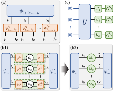
Figure 1: (a) The graphical representation of the 2-layer HTTNs expressed by Eq. (3). The upper quantum tensor $\psi_{i_{1},i_{2},...,i_{N}}=\braket{i_{1}i_{2}...i_{N}}{U}{0^{N}}$ represents the non-local correlation between the subsystems, and the lower quantum tensor $\psi_{j_{1},...,j_{K}}^{i_{k}}=\braket{j_{1}...j_{N}}{\psi_{k}^{i_{k}}}$($k=1,...,N$) represents a quantum state of each subsystem. When calculating the expectation value of observable $O=\bigotimes_{k=1}^{N}O_{k}$ for $\ket{\psi_{\rm HT}}$, (b1) we first contract the local quantum systems (green area) and then (b2) obtain Hermitian operators $\{M_{k}\}_{k=1}^{N}$. Using the quantum circuit in (c) corresponding to the diagram of (b2), we complete the contraction of the whole system.

Here, we review hybrid tree tensor networks (HTTNs) as an important class of HTNs. The $2$-layer tree TN state consisting of quantum tensors can be expressed by

$$\ket{\psi_{\rm HT}}=\frac{1}{C}\sum_{i_{1},...,i_{N}}\psi_{i_{1},...,i_{N}}\ket{\psi^{i_{1}}_{1}}\otimes...\otimes\ket{\psi^{i_{N}}_{N}}.$$ (3)

Let $\ket{\psi^{i_{k}}_{k}}(k=1,...,N)$ be a $K$-qubit quantum tensor, $\psi_{i_{1},...,i_{N}}=\braket{i_{1},...,i_{2}}{\psi}$ be the probability ampulitude of a $N$-qubit system, and $C$ be a normalization constant, $\ket{\psi_{\rm HT}}$ is an $NK$-qubit system. The expectation values of observables for $\ket{\psi_{\rm HT}}$ can be computed only with a $\mathrm{max}\{N,K\}$-qubit system. Denote an $NK$-qubit observable as $O=\bigotimes_{k=1}^{N}O_{k}$ for a $K$-qubit observable $O_{k}$. Then, we obtain the expectation value including the normalization constant as follows:

$$\braket{O}_{\psi_{\rm HT}} ={\frac{1}{C^{2}}}\sum_{\vec{i},\vec{i}^{\prime}}\psi_{\vec{i}}^{*}\psi_{\vec{i}^{\prime}}\prod_{k=1}^{N}M_{k}^{i_{k},i_{k}^{\prime}}$$ (4)

$$=\frac{1}{C^{2}}\bra{\psi}\bigotimes_{k=1}^{N}M_{k}\ket{\psi}$$

and

$$C^{2} =\sum_{\vec{i},\vec{i}^{\prime}}\psi_{\vec{i}}^{*}\psi_{\vec{i}^{\prime}}\prod_{k=1}^{N}S_{k}^{i_{k},i_{k}^{\prime}}$$ (5)

$$=\bra{\psi}\bigotimes_{k=1}^{N}S_{k}\ket{\psi},$$

where $\vec{i}=(i_{1},i_{2},...i_{N})$, $\vec{i}^{\prime}=(i_{1}^{\prime},i_{2}^{\prime},...i_{N}^{\prime})$, $M_{k}^{i_{k},i_{k}^{\prime}}=\bra{\psi_{k}^{i_{k}}}O_{k}\ket{\psi_{k}^{i_{k}^{\prime}}}$ and $S_{k}^{i_{k},i_{k}^{\prime}}=\braket{\psi_{k}^{i_{k}}}{\psi_{k}^{i_{k}^{\prime}}}$. Therefore, $\braket{O}_{\psi_{\rm HT}}$ can be evaluated as follows. First, we calculate $\{M_{k}\}_{k=1}^{N}$ ($\{S_{k}\}_{k=1}^{N}$) via contractions of local quantum tensors $\{\ket{\psi^{i_{k}}}_{k}\}_{k}$. Then, because $\{M_{k}\}_{k}$ ($\{S_{k}\}_{k}$) are Hermitian operators, we have the spectral decomposition $M_{k}=U_{k}^{\dagger}\Lambda_{k}U_{k}$ ($S_{k}=V_{k}^{\dagger}\Lambda^{\prime}_{k}V_{k}$) for a unitary operator $U_{k}$ ($V_{k}$) and a diagonal operator $\Lambda_{k}$ ($\Lambda^{\prime}_{k}$). Thus, by applying $\otimes_{k=1}^{N}U_{k}$ immediately before measurement and measuring on the $Z$ basis and assigning the elements of $\Lambda_{k}$ ($\Lambda^{\prime}_{k}$) to the measurement outcomes, we can measure the expectation value of $\bigotimes_{k=1}^{N}M_{k}$ ($\bigotimes_{k=1}^{N}S_{k}$) for the state $\ket{\psi}$. A graphical diagram for the procedure of contractions is shown in Fig. 1. For the contraction rule for the transition amplitudes $\bra{\psi^{\prime}_{\rm HT}}O\ket{\psi_{\rm HT}}$ for different hybrid tensors $\ket{\psi_{\rm HT}}$ and $\ket{\psi^{\prime}_{\rm HT}}$, refer to Kanno et al. [19]. While we considered the HTN state comprising only quantum tensors above, note that we can also consider the HTN model where quantum tensors and classical tensors are used interchangeably [18].

The efficiency of calculating each $M_{k}(S_{k})$ is highly dependent on the way of preparing a set of quantum states $\{\ket{\psi_{k}^{i_{k}}}\}_{i_{k}}$. To see the detailed procedures for computing $M_{k}(S_{k})$, we consider the more general scenario where one contracts the $K$-qubit local tensor $\psi_{k}^{\vec{i}_{k}}$, which is connected to the index $\vec{i}_{k}\in\{0,1\}^{\tau}$ of its parent tensor, and the local observable $O_{k}$ to obtain $M_{k}^{\vec{i}_{k},\vec{i}^{\prime}_{k}}=\braket{\psi_{k}^{\vec{i}_{k}}}{O_{k}}{\psi_{k}^{\vec{i}^{\prime}_{k}}}$. When $\psi^{\vec{i}_{k}}$ is a classical tensor (i.e., the set of states $\{\ket{\psi_{k}^{\vec{i}_{k}}}\}_{\vec{i}_{k}}$ is prepared by classical computers), we calculate each element of $M_{k}(S_{k})$ on classical computers. For example, if we use the MPS representation to express the local tensor as $\ket{\psi_{k}^{\vec{i}_{k}}}=\sum_{j_{1},j_{2},...,j_{K}}\mathrm{Tr}[A_{1}^{\vec{i}_{k},j_{1}}A_{2}^{j_{2}}...A_{K}^{j_{K}}]\ket{j_{1},j_{2},...,j_{K}}$, we obtain matrix elements $M_{k}^{\vec{i}_{k},\vec{i}^{\prime}_{k}}=\braket{\psi_{k}^{\vec{i}_{k}}}{O_{k}}{\psi_{k}^{\vec{i}^{\prime}_{k}}}$ by a classical contraction of the MPS state. Meanwhile, when $\psi^{\vec{i}_{k}}$ is a quantum tensor (i.e., the set of states $\{\ket{\psi_{k}^{\vec{i}_{k}}}\}_{\vec{i}_{k}}$ is prepared by quantum computers), we calculate $M_{k}(S_{k})$ by performing measurements on a quantum computer. Since the specific calculation varies depending on the definition of $\{\ket{\psi_{k}^{\vec{i}_{k}}}\}_{\vec{i}_{k}}$, we explain the computation procedures to obtain $M_{k}(S_{k})$ for the following four cases, where the index $\vec{i}_{k}$ is associated with

(i) initial states

$\ket{\psi_{k}^{\vec{i}_{k}}}=U_{k}\ket{\vec{i}_{k}}\ket{\vec{0}}$

(ii) projections

$\ket{\psi_{k}^{\vec{i}_{k}}}=\braket{\vec{i}_{k}}{\psi_{k}}$,

(iii) Pauli operators

$\ket{\psi_{k}^{\vec{i}_{k}}}=P_{k}^{\vec{i}_{k}}\ket{\psi_{k}}$,

(iv) unitary gates

$\ket{\psi_{k}^{\vec{i}_{k}}}=U_{k}^{\vec{i}_{k}}\ket{\vec{0}}$.

Note that although certain types can be represented in the framework of another type from a mathematical perspective (e.g., type (i) and (iii) can be regarded as special examples of type (iv)), we distinguish each type for the practical reason that different characterizations of the state $\ket{\psi^{\vec{i}_{k}}_{k}}$ by $\vec{i}_{k}$ require the different quantum circuits and the procedure to calculate the $M_{k}(S_{k})$.

II.1 Calculation of $M_{k}$ and $S_{k}$ in Type (i)

In the case of $\ket{\psi_{k}^{\vec{i}_{k}}}=U_{k}\ket{\vec{i}_{k}}\ket{\vec{0}}$, each element of the Hermitian matrix $M_{k}$ is represented as

$$M_{k}^{\vec{i}_{k},\vec{i}^{\prime}_{k}}=\mathrm{Tr}\left[O_{k}\,\mathcal{U}_{k}\left(\ket{\vec{i}^{\prime}_{k}}\bra{\vec{i}_{k}}\otimes\ket{\vec{0}}\bra{\vec{0}}\right)\right],$$ (6)

where $\mathcal{U}_{k}(\bullet)=U_{k}\bullet U_{k}^{\dagger}$ is a $K$-qubit unitary channel. Here, let us define $E_{k}(\ket{a_{k}})=\mathrm{Tr}[O_{k}\,\mathcal{U}_{k}(\ket{a_{k}}\bra{a_{k}}\otimes\ket{\vec{0}}\bra{\vec{0}})]$. Since $\ket{\vec{i}^{\prime}_{k}}\bra{\vec{i}_{k}}$ can be expressed by a linear combination of the eigenstates of the Pauli operators, we can calculate each element of $M_{k}$ by appropriately combining the measurement results $E_{k}(\ket{a_{k}})$ for various inputs $\ket{a_{k}}$. In the following, we will use the case of $\tau=1$ as an example. First, we obtain the diagonal elements of $M_{k}$, by measuring the expectation values of the observable $O_{k}$ for the states prepared by the quantum circuit in Fig. 2(a) with the input state $\ket{a_{k}}$ being $\ket{0}$ and $\ket{1}$, i.e., $M_{k}^{0,0}=E_{k}(\ket{0})$ and $M_{k}^{1,1}=E_{k}(\ket{1})$. Next, we calculate the off-diagonal elements of $M_{k}$ by using the quantum circuit in Fig. 2(a) as

$$M_{k}^{0,1}=\frac{E_{k}(\ket{+})-E_{k}(\ket{-})-i\{E_{k}(\ket{+i})-E_{k}(\ket{-i})\}}{2}$$ (7)

and $M_{k}^{1,0}=M_{k}^{0,1\ast}$. Here, we define $\ket{+},\ket{-},\ket{+i},$ and $\ket{-i}$ as the eigenvectors with eigenvalues $+1$ and $-1$ of Pauli operators $X$ and $Y$, respectively. Noticing that $E_{k}(\ket{0})+E_{k}(\ket{1})=E_{k}(\ket{+})+E_{k}(\ket{-})=E_{k}(\ket{+i})+E_{k}(\ket{-i})$, we can reuse the calculation results $E_{k}(\ket{0})$ and $E_{k}(\ket{1})$ used in the estimation of the diagonal elements to calculate $M_{k}^{0,1}$, that is,

$$M_{k}^{0,1}=E_{k}(\ket{+})-iE_{k}(\ket{+i})+\frac{i-1}{2}\{E_{k}(\ket{0})+E_{k}(\ket{1})\}.$$ (8)

This modification allows a reduction from six to four in the number of distinct input states needed for the estimation of $M$.

We do not need to calculate the matrix $M_{Ak}$ because it holds that $S_{k}=I$ for any $k$, and consequently $C^{2}=1$ holds.

II.2 Calculation of $M_{k}$ and $S_{k}$ in Type (ii)

In the case of $\ket{\psi_{k}^{\vec{i}_{k}}}=\braket{\vec{i}_{k}}{\psi_{k}}$ where $\ket{\psi_{k}}$ is a $(K+\tau)$-qubit state, each element of the Hermitian matrix $M_{k}$ is represented as

$$M_{k}^{\vec{i}_{k},\vec{i}^{\prime}_{k}}=\mathrm{Tr}\left[\left(\ket{\vec{i}_{k}}\bra{\vec{i}^{\prime}_{k}}\otimes O_{k}\right)\mathcal{U}_{k}(\ket{\vec{0}}\bra{\vec{0}})\right],$$ (9)

where $\mathcal{U}_{k}(\ket{\vec{0}}\bra{\vec{0}})$ is a $(K+\tau)$-qubit quantum channel operating as $\mathcal{U}_{k}(\ket{\vec{0}}\bra{\vec{0}})=\ket{\psi_{k}}\bra{\psi_{k}}$. Since $\ket{\vec{i}_{k}}\bra{\vec{i}^{\prime}_{k}}$ can be decomposed into a linear combination of the Pauli operators, we can estimate each element of $M_{k}$ by combining the measurement results $E_{k}(\omega_{k})=\mathrm{Tr}\left[\left(\omega_{k}\otimes O_{k}\right)\mathcal{U}_{k}(\ket{\vec{0}}\bra{\vec{0}})\right]$ for various Pauli observables $\omega_{k}\in\{I,X,Y,Z\}^{\otimes\tau}$. In the following, we will use the case of $\tau=1$ as an example. We can estimate the diagonal elements $M_{k}^{0,0}$ and $M_{k}^{1,1}$ by measuring the expectation values of $\omega_{k}\otimes O_{k}(\omega_{k}=I,Z)$ for the state $\ket{\psi_{k}}\bra{\psi_{k}}$ prepared by the quantum circuit in Fig. 2(b), i.e., $M_{k}^{0,0}=\{E_{k}(I)+E_{k}(Z)\}/2$ and $M_{k}^{1,1}=\{E_{k}(I)-E_{k}(Z)\}/2$. From the linearity of $E_{k}(\omega_{k})$, the off-diagonal elements can be obtained as $M_{k}^{0,1}=\{E_{k}(X)+iE_{k}(Y)\}/2$ and $M_{k}^{1,0}=M_{k}^{0,1\ast}$. In the same way, we can calculate $S_{k}$ by replacing $O_{k}$ with $I$ in the calculation of $M_{k}$.

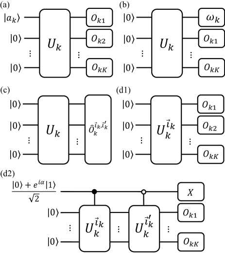
Figure 2: Quantum circuits for obtaining $M_{k}$ from type (i) to (iv). $S_{k}$ can be similarly obtained by replacing $O_{k}=\otimes_{m=1}^{K}O_{km}$ with $I^{\otimes K}$ from types (ii) to (iv). (a) A quantum circuit for calculating $M_{k}$ in the case of $\ket{\psi_{k}^{i_{k}}}=U_{k}\ket{i_{k}}\ket{\vec{0}}$. Each element of $M_{k}$ can be obtained by preparing input states $\ket{a_{k}}$ as $\ket{0}$, $\ket{1}$, $\ket{+},\ket{-}$, $\ket{+i}$, and $\ket{-i}$, evaluating $E(\ket{a_{k}})$, and combining those results as Eq. (7) (otherwise, preparing $\ket{a_{k}}$ as $\ket{0}$, $\ket{1}$, $\ket{+}$, and $\ket{+i}$, for Eq. (8)) (b) A quantum circuit for calculating $M_{k}$ in the case of $\ket{\psi_{k}^{i_{k}}}=\braket{i_{k}}{\psi_{k}}$. $U_{k}$ is a unitary gate working as $\ket{\psi_{k}}=U_{k}\ket{0}^{\otimes K+1}$, and $\omega_{k}$ takes $I$, $X$, $Y$, and $Z$. (c) A quantum circuit for calculating $M_{k}$ in the case of $\ket{\psi_{k}^{\vec{i}_{k}}}=P_{k}^{\vec{i}_{k}}\ket{\psi_{k}}$. $U_{k}$ is a unitary gate working as $\ket{\psi_{k}}=U_{k}\ket{0}^{\otimes K}$. (d1) A quantum circuit for calculating diagonal elements $M_{k}^{\vec{i}_{k},\vec{i}_{k}}$, and (d2) a circuit for calculating off-diagonal elements $M_{k}^{\vec{i}_{k},\vec{i}_{k}^{\prime}}$. A controlled-$U_{k}^{\vec{i}_{k}}$ (controlled-$U_{k}^{\vec{i}^{\prime}_{k}}$) with a black (white) circle works on the target qubits when the control qubit is $\ket{1}$ ($\ket{0}$).

II.3 Calculation of $M_{k}$ and $S_{k}$ in Type (iii)

In the case of $\ket{\psi_{k}^{\vec{i}_{k}}}=P_{k}^{\vec{i}_{k}}\ket{\psi_{k}}$ where $P_{k}^{\vec{i}_{k}}\in\{I,X,Y,Z\}^{\otimes K}$ is a tensor product of the Pauli operators, each element of the Hermitian matrix $M_{k}$ is represented as

$$M_{k}^{\vec{i}_{k},\vec{i}^{\prime}_{k}}=\mathrm{Tr}\left(\hat{O}_{\vec{i}_{k},\vec{i}^{\prime}_{k}}\,\mathcal{U}_{k}(\ket{\vec{0}}\bra{\vec{0}})\right),$$ (10)

where $\mathcal{U}_{k}(\ket{\vec{0}}\bra{\vec{0}})$ is a $K$-qubit quantum channel working as $\mathcal{U}_{k}(\ket{\vec{0}}\bra{\vec{0}})=\ket{\psi_{k}}\bra{\psi_{k}}$, and $\hat{O}_{\vec{i}_{k},\vec{i}^{\prime}_{k}}=P_{k}^{\vec{i}_{k}}O_{k}P_{k}^{\vec{i}^{\prime}_{k}}$. We can evaluate $M_{k}^{\vec{i}_{k},\vec{i}^{\prime}_{k}}$ with direct measurements of Pauli operators $P_{l_{k}}$, by decomposing the observable $\hat{O}_{\vec{i}_{k},\vec{i}^{\prime}_{k}}$ into a linear combination of the Pauli operators as $\hat{O}_{\vec{i}_{k},\vec{i}^{\prime}_{k}}=\sum_{l_{k}}f_{l_{k}}P_{l_{k}}$ (Fig. 2(c)), and also obtain $M_{k}^{\vec{i}^{\prime}_{k},\vec{i}_{k}}$ by $M_{k}^{\vec{i}^{\prime}_{k},\vec{i}_{k}}=M_{k}^{\vec{i}_{k},\vec{i}^{\prime}_{k}\ast}$. For the calculation of $S_{k}$, each diagonal element $S_{k}^{\vec{i}_{k},\vec{i}^{\prime}_{k}}$ is 1. Each off-diagonal element $S_{k}^{\vec{i}_{k},\vec{i}^{\prime}_{k}}$ can be calculated by directly measuring the Pauli observable $P^{\vec{i}_{k}}P^{\vec{i}^{\prime}_{k}}$ for the state $\ket{\psi_{k}}\bra{\psi_{k}}$.

II.4 Calculation of $M_{k}$ and $S_{k}$ in Type (iv)

In the case of $\ket{\psi_{k}^{\vec{i}_{k}}}=U_{k}^{\vec{i}_{k}}\ket{\vec{0}}$, each element of the Hermitian matrix $M_{k}$ is represented as

$$M_{k}^{\vec{i}_{k},\vec{i}^{\prime}_{k}}=\mathrm{Tr}\left[O_{k}U_{k}^{\vec{i}^{\prime}_{k}}\ket{\vec{0}}\bra{\vec{0}}U_{k}^{\vec{i}_{k}\dagger}\right].$$ (11)

To estimate diagonal elements $M_{k}^{\vec{i}_{k},\vec{i}_{k}}$, we only need to measure the expectation value of the observable $O_{k}$ for the state $\ket{\psi_{k}^{\vec{i}_{k}}}\bra{\psi_{k}^{\vec{i}_{k}}}=\mathcal{U}_{k}^{\vec{i}_{k}}(\ket{\vec{0}}\bra{\vec{0}})$ as shown in Fig. 2(d1). Next, we consider the procedure for estimating off-diagonal elements of $M_{k}$. The quantum circuit to estimate $M_{k}^{\vec{i}_{k},\vec{i}^{\prime}_{k}}$ is shown in Fig. 2(d2). Now, we set the initial state as $\frac{\ket{0}+e^{i\alpha}\ket{1}}{\sqrt{2}}\otimes\ket{0}^{K}$ where $\alpha$ is the phase. When setting $\alpha=0$ for the parameterized initial state, we obtain Re$(M_{k}^{\vec{i}_{k},\vec{i}^{\prime}_{k}})$ by measuring the expectation value $\braket{X\otimes O}$. Similarly, we obtain Im$(M_{k}^{\vec{i}_{k},\vec{i}^{\prime}_{k}})$ by setting $\alpha=\frac{\pi}{2}$ and calculating the expectation value $\braket{X\otimes O}$. Combining the real and imaginary parts, we obtain $M_{k}^{\vec{i}_{k},\vec{i}^{\prime}_{k}}$, and $M_{k}^{\vec{i}^{\prime}_{k},\vec{i}_{k}}=M_{k}^{\vec{i}_{k},\vec{i}^{\prime}_{k}\ast}$. To estimate the matrix $S_{k}$, we set the diagonal terms as 1 and estimate off-diagonal elements by substituting $O_{k}$ for $I$ of the above procedure.

III Techniques relevant to hybrid tensor networks

To simulate large quantum systems by exploiting devices with limited quality and quantity of qubits, many new algorithms have been recently proposed [32, 12, 13, 14, 15, 16, 17, 18, 19, 20, 33, 34, 35, 36, 37]. While these algorithms differ from the specific implementation of quantum circuits and the way of classical processing, they share the idea of simulating a larger quantum system by dividing the system into some clusters with strong internal interaction but weak interaction among them. From another perspective, they also have in common that their basic concepts are closely related to the conventional TN approaches [22, 23, 24, 25, 26]. In this section, we overview Deep VQE [15] and entanglement forging [12] as representative examples of such algorithms and formalize these algorithms from the framework of HTNs [18].

III.1 Deep VQE

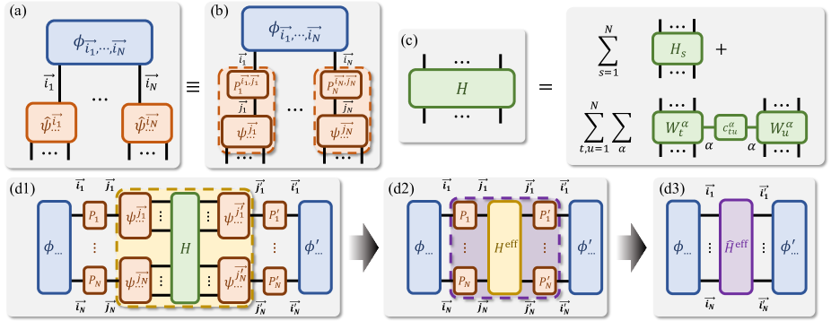
Figure 3: The HTN representation of Deep VQE algorithm. (a) The graphical representation of the HTTN state $\ket{\psi_{\rm DV}}$, expressed by Eq. (24). Note that $\vec{i}_{s}$ of $\ket{\widehat{\psi}_{s}^{\vec{i}_{s}}}$ in Eq. (24) corresponds to $m_{s}$ of $\ket{\widehat{\psi}_{s}^{m_{s}}}$ defined in Eq. (13), as $m_{s}=(\vec{j}_{s})_{(10)}$ and $\ket{\widehat{\psi}_{s}^{\vec{j}_{s}}}=\vec{0}$ for $(\vec{j}_{s})_{(10)}\geq K_{s}$. (b) The graphical representation of the HTTN state defined in Eq. (26). The $s$-th classical tensor $P_{s}^{\vec{i}_{s},\vec{j}_{s}}$ is calculated so that the $s$-th set of states $\{\ket{\widehat{\psi}^{\vec{i}_{s}}_{s}}\}_{\vec{i}_{s}}$ forms the orthonormal basis of the $s$-th subsystem, where $\ket{\widehat{\psi}^{\vec{i}_{s}}_{s}}$ is represented as a linear combination of the un-normalized states $\{\ket{\psi_{s}^{\vec{j}_{s}}}\}_{\vec{j}_{s}}$, i.e., $\ket{\widehat{\psi}^{\vec{i}_{s}}_{s}}=\sum_{\vec{j}_{s}}P_{s}^{\vec{i}_{s},\vec{j}_{s}}\ket{\psi_{s}^{\vec{j}_{s}}}$. (c) The tensor representation of the Hamiltonian defined in Eq. (12). (d) The schematic diagram of the calculation of the expectation value of the Hamiltonian $H$ for the HTTN state $\ket{\psi_{\rm DV}}$. By contracting the local quantum tensors $\psi_{s}^{\vec{j}_{s}}$, $\psi_{s}^{\vec{j}^{\prime}_{s}}$, and the classical tensor $H$ (yellow area in (d1)), we obtain an contracted tensor $H^{\rm eff}$, corresponding to the un-normalized effective Hamiltonian in Deep VQE. Then, by contracting the effective Hamiltonian $H^{\rm eff}$ and the classical tensors $P_{s}^{\vec{i}_{s},\vec{j}_{s}}$, and $P_{s}^{\vec{i}^{\prime}_{s},\vec{j}^{\prime}_{s}}$ (purple area in (d2)), we obtain a new tensor $\widehat{H}^{\mathrm{eff}}$, which is the normalized effective Hamiltonian in Deep VQE. Finally, contracting the whole system in (d3) using a quantum computer, we obtain $\braket{H}_{\psi_{\rm DV}}$

.

Let us consider $n_{\rm tot}$-qubit quantum state composed of $N$ subsystems and the $s$-th subsystem consists of $n_{s}$ qubits, i.e., $n_{\rm tot}=\sum_{s=1}^{N}n_{s}$. Note that we are focusing on the following situation: the whole system can be divided into the $N$ clusters with strong internal interactions but weak interaction between them. Then, the Hamiltonian can be written as

$$H=\sum_{s=1}^{N}H_{s}+\sum_{t,u=1}^{N}V_{tu},\quad V_{tu}=\sum_{\alpha}c_{tu}^{\alpha}W^{\alpha}_{t}\otimes W^{\alpha}_{u}$$ (12)

where $H_{s}$ corresponds to the $s$-th subsystem’s Hamiltonian and $V_{tu}$ to the inter-subsystem Hamiltonian acting on the $s$-th and $t$-th subsystems. Here, the interaction term $V_{tu}$ is decomposed into the linear sum of the tensor products of $W^{\alpha}_{t}$ and $W^{\alpha}_{u}$ acting on the $t$-th and the $u$-th subsystems with the coefficients $c_{tu}^{\alpha}$. The Deep VQE algorithm is roughly comprised of four steps, each of which is described as follows.

The first step of this algorithm is to find the ground state of each subsystem’s Hamiltonian $H_{s}$ by the conventional VQE approach, minimizing the expectation value of $H_{s}$ by optimizing the parameters $\vec{\theta}^{(s)}$ in each quantum state $\ket{\psi_{s}}=U^{(s)}(\vec{\theta}^{(s)})\ket{0^{n_{s}}}$. Hereafter, let $\ket{\psi_{s}^{\mathrm{G}}}=U^{(s)}(\vec{\theta}^{(s)\star})\ket{0^{n_{s}}}$ be the approximated ground state, where $\vec{\theta}^{(s)\star}$ is an optimized parameter set of the subsystem $s$.

In the second step, we generate the $K_{s}$-dimensional orthonormal local basis $\{\ket{\widehat{\psi}_{s}^{m}}\}_{m=0}^{K_{s}-1}$ on the basis of the ground state $\ket{\psi_{s}^{\rm G}}$. First, we construct non-orthonormal local basis $\{\ket{{\psi}_{s}^{m}}\}_{m=0}^{K_{s}-1}$ as

$$\ket{\psi_{s}^{m}}=D_{s}^{m}\ket{\psi_{s}^{\mathrm{G}}},$$ (13)

where $D_{s}^{m}$ denotes the $2^{n_{s}}\times 2^{n_{s}}$ local excitation operator on the $s$-th subsystem, and $D_{s}^{0}$ is an identity operator. Fujii et al. [15] pointed out that when the number of dimensions $K_{s}$ is fixed, one of the proper choices of $D_{s}^{0}$ is assigning the local excitation $D_{s}^{m}$ to $W_{s}^{m}$ at the boundary . In this review part, following the original research [15], we choose $D_{s}^{m}$ as $W_{s}^{m}$. Then, we define the orthonormal local basis $\{\ket{\widehat{\psi}_{s}^{m}}\}_{m=0}^{K_{s}-1}$ using the Gram-Schmidt procedure for $\{\ket{{\psi}_{s}^{m}}\}_{m=0}^{K_{s}-1}$:

$$\ket{\widehat{\psi}_{s}^{m}}=\frac{\ket{{\psi}_{s}^{m}}-\sum_{l<m}\braket{\widehat{\psi}_{s}^{l}}{{\psi}_{s}^{m}}\ket{\widehat{\psi}_{s}^{l}}}{\|\ket{{\psi}_{s}^{m}}-\sum_{l<m}\braket{\widehat{\psi}_{s}^{l}}{{\psi}_{s}^{m}}\ket{\widehat{\psi}_{s}^{l}}\|}.$$ (14)

From Eq. (14), the matrix $P_{s}$, which transforms the basis $\{\ket{{\psi}_{s}^{m}}\}_{m=0}^{K_{s}-1}$ to the orthonormalized basis $\{\ket{\widehat{\psi}_{s}^{m}}\}_{m=0}^{K_{s}-1}$, can be determined as

$$\ket{\widehat{\psi}_{s}^{m}}=\sum_{m^{\prime}=0}^{K_{s}-1}P^{mm^{\prime}}_{s}\ket{\psi_{s}^{m^{\prime}}}.$$ (15)

Each matrix element $P^{mm^{\prime}}_{s}$ can be calculated, by exploiting a set of inner products of local basis $\{\braket{\psi_{s}^{l}}{\psi_{s}^{m}}\}_{l,m}$. Here, each inner product $\braket{\psi_{s}^{l}}{\psi_{s}^{m}}$ can be calculated with direct measurement because it can be expressed as

$$\braket{\psi_{s}^{\mathrm{G}}}{{W_{s}^{l}}^{\dagger}W_{s}^{m}}{\psi_{s}^{\mathrm{G}}}$$ (16)

and the operator ${W_{s}^{l}}^{\dagger}W_{s}^{m}$ can be decomposed into a linear combination of Hermitian operators. The matrix $P_{s}$ formulated above is needed to normalize the effective Hamiltonian in the next step.

In the third step, we construct the normalized effective Hamiltonian on the basis of the orthonormal basis $\{\ket{\widehat{\psi}_{s}^{m}}\}_{m=0}^{K_{s}-1}$. The normalized effective Hamiltonian $H_{s}^{\mathrm{eff}}$ for the $s$-th subsystem is defined as

$$(\widehat{H}_{s}^{\mathrm{eff}})^{lm}:=\braket{\widehat{\psi}^{l}_{s}}{H_{s}}{\widehat{\psi}^{m}_{s}}.$$ (17)

Note that terms that can be directly measured on quantum computers are un-normalized ones $(H_{s}^{\mathrm{eff}})^{lm}:=\braket{\psi^{l}_{s}}{H_{s}}{\psi^{m}_{s}}$. Thus, we first evaluate

$$(H_{s}^{\mathrm{eff}})^{lm}=\braket{\psi_{s}^{\mathrm{G}}}{{W_{s}^{l}}^{\dagger}H_{s}W_{s}^{m}}{\psi_{s}^{\mathrm{G}}},$$ (18)

by decomposing the operator ${W_{s}^{l}}^{\dagger}H_{s}W_{s}^{m}$ into a linear combination Hermitian operator and performing the direct measurement. Then, we transform $(H_{s}^{\rm eff})^{lm}$ into the normalized effective Hamiltonian $(\widehat{H}_{s}^{\mathrm{eff}})^{lm}$, by applying the matrix $P_{s}$ to $(H_{s}^{\mathrm{eff}})^{lm}$ as

$$\begin{split}(\widehat{H}_{s}^{\mathrm{eff}})^{lm}&=\sum_{l^{\prime}=0}^{K_{s}-1}\sum_{m^{\prime}=0}^{K_{s}-1}{P^{ll^{\prime}}_{s}}^{\ast}\braket{\psi^{l^{\prime}}_{s}}{H_{s}}{\psi^{m^{\prime}}_{s}}P^{mm^{\prime}}_{s}\\ &=\left({P_{s}}^{\ast}H_{s}^{\mathrm{eff}}{P_{s}}^{\rm T}\right)^{lm},\end{split}$$ (19)

where $\ast$ and $\mathrm{T}$ denote the complex conjugate and transposition of matrices. Similarly, the normalized effective interaction Hamiltonian $\widehat{V}_{tu}^{\mathrm{eff}}$ is defined as

$$(\widehat{V}_{tu}^{\mathrm{eff}})^{abcd}:=\bra{\widehat{\psi}^{a}_{t}}\bra{\widehat{\psi}^{b}_{u}}V_{tu}\ket{\widehat{\psi}^{c}_{t}}\ket{\widehat{\psi}^{d}_{u}}.$$ (20)

Since $V_{tu}$ can be decomposed into the tensor products of the local Hamiltonian acting on the $t$-th and $u$-th subsystems as Eq. (12), un-normalized effective interaction Hamiltonian $(V^{\mathrm{eff}}_{tu})^{abcd}:=\bra{\psi^{a}_{t}}\bra{\psi^{b}_{u}}V_{tu}\ket{\psi^{c}_{t}}\ket{\psi^{d}_{u}}$ can be derived from integrating the expectation value of each subsystem. Then, applying the matrices $P_{t}$ and $P_{u}$ to $(V^{\mathrm{eff}}_{tu})_{abcd}$, we obtain the normalized effective interaction Hamiltonian as

$$(\widehat{V}_{tu}^{\mathrm{eff}})^{abcd}=\sum_{\alpha}c_{tu}^{\alpha}(\widehat{W}_{t}^{\alpha^{\mathrm{eff}}})^{ac}(\widehat{W}_{u}^{\alpha^{\mathrm{eff}}})^{bd}.$$ (21)

The normalized effective Hamiltonian $(\widehat{W}_{t}^{\alpha^{\mathrm{eff}}})^{ac}$ and $(\widehat{W}_{u}^{\alpha^{\mathrm{eff}}})^{bd}$ can be calculated in the same way as Eq. (19). After calculating $(\widehat{H}_{s}^{\mathrm{eff}})^{lm}$ and $(\widehat{V}_{tu}^{\mathrm{eff}})^{abcd}$, we can convert the original Hamiltonian $H$ into the normalized effective one as

$$\widehat{H}^{\mathrm{eff}}=\sum_{s=1}^{N}\widehat{H}_{s}^{\mathrm{eff}}+\sum_{t,u=1}^{N}\widehat{V}_{tu}^{\mathrm{eff}}.$$ (22)

In the fourth step, we estimate the ground state for the effective Hamiltonian $\widehat{H}^{\mathrm{eff}}$ by the typical VQE with the $\kappa$-qubit parameterized quantum circuit $V(\vec{\,\eta})$ in which $\kappa:=\sum_{s=1}^{N}\kappa_{s}$ with $\kappa_{s}:=\lceil\log_{2}K_{s}\rceil$. The expectation value of the effective Hamiltonian $\widehat{H}^{\mathrm{eff}}$ for the approximated ground state $V(\vec{\,\eta}^{\star})\ket{0^{\kappa}}$ approximates the ground state energy $E_{\rm min}$ for the original Hamiltonian $H$:

$$E_{\rm min}\simeq\braket{0^{\kappa}}{V(\vec{\,\eta}^{\star})^{\dagger}\widehat{H}^{\mathrm{eff}}V(\vec{\,\eta}^{\star})}{0^{\kappa}}.$$ (23)

One of the notable points of this technique is that it only takes $\max(n_{s},\kappa)$ qubits to simulate a $n_{\rm tot}$-qubit quantum system. Furthermore, by repeating the series of steps, we can simulate even larger-scale systems.

Having viewed a series of procedures of the Deep VQE following the description in Fujii et al. [15], we characterize this algorithm from the view of the HTNs. First, the HTTN state constructed by the Deep VQE can be represented as

$$\ket{\psi_{\rm DV}}=\sum_{\vec{i}_{1},...,\vec{i}_{N}}\phi_{\vec{i}_{1},...,\vec{i}_{N}}\ket{\widehat{\psi}_{1}^{\vec{i}_{1}}}\otimes...\otimes\ket{\widehat{\psi}_{N}^{\vec{i}_{N}}},$$ (24)

where $\phi_{\vec{i}_{1},...,\vec{i}_{N}}=\braket{\vec{i}_{1},...,\vec{i}_{N}}{V(\vec{\eta})}{0^{\kappa}}$ is the $\kappa$-qubit quantum tensor representing the correlations between subsystems with the quantum indices $\vec{i}_{s}=(i_{s1},...,i_{s\kappa_{s}})\in\{0,1\}^{\kappa_{s}}$ ($s=1,...,N$), and $\{\ket{\widehat{\psi}_{s}^{\vec{i}^{\prime}_{s}}}\}_{\vec{i}^{\prime}_{s}}$ is the $s$-th set of $n_{s}$-qubit quantum states with the classical index $\vec{i}^{\prime}_{s}\in\{0,1\}^{\kappa_{s}}$. A graphical picture of Eq. (24) is depicted in Fig. 3(a). Here, each state $\ket{\widehat{\psi}^{\vec{i}_{s}}_{s}}$ can be expanded as a linear combination of quantum states $\ket{\psi_{s}^{\vec{j}_{s}}}$ with classical coefficients $P_{s}^{\vec{i}_{s},\vec{j}_{s}}$, i.e., $\ket{\widehat{\psi}^{\vec{i}_{s}}_{s}}=\sum_{\vec{j}_{s}}P_{s}^{\vec{i}_{s},\vec{j}_{s}}\ket{\psi_{s}^{\vec{j}_{s}}}$, where each set of states $\{\ket{\psi_{s}^{\vec{j}^{\prime}_{s}}}\}_{\vec{j}^{\prime}_{s}}$ is prepared by quantum computers with type (iii) state preparations:

$$\ket{\psi_{s}^{\vec{j}^{\prime}_{s}}}=\begin{cases}W^{\vec{j}^{\prime}_{s}}_{s}\ket{\psi_{s}^{\mathrm{G}}},&(\vec{j}^{\prime}_{s})_{(10)}\leq K_{s}-1,\\ \vec{0},&(\vec{j}^{\prime}_{s})_{(10)}\geq K_{s},\end{cases}$$ (25)

where $(\vec{i}_{s})_{(10)}(s=1,...,N)$ are the decimal representations of the binary indices $\vec{i}_{s}$, and $W^{\vec{j}_{s}}_{s}$ are the $2^{n_{s}}\times 2^{n_{s}}$ local excitation operators. Then, we can rewrite Eq. (24) as

$$\ket{\psi_{\rm DV}}=\sum_{\begin{subarray}{c}\vec{i}_{1},...,\vec{i}_{N}\\ \vec{j}_{1},...,\vec{j}_{N}\end{subarray}}\phi_{\vec{i}_{1},...,\vec{i}_{N}}P_{1}^{\vec{i}_{1},\vec{j}_{1}}\ket{\psi_{1}^{\vec{j}_{1}}}\otimes...\otimes P_{N}^{\vec{i}_{N},\vec{j}_{N}}\ket{\psi_{N}^{\vec{j}_{N}}},$$ (26)

and the graphical figure of Eq. (26) is shown in Fig. 3(b).

Next, we elaborate on the way of obtaining the expectation value of the Hamiltonian $H$ for the state $\ket{\psi_{\rm DV}}$, i.e., $\braket{\psi_{\rm DV}}{H}{\psi_{\rm DV}}$, through contraction of the indices of HTTN state in Eq. (26). The contraction process consists of three main steps. In the first step, we contract the quantum tensors $\psi_{s}^{\vec{j}_{s}}$, $\psi_{s}^{\vec{j}^{\prime}_{s}}$, and the classical tensor $H$ (Fig. 3(d1)), and we obtain a new Hamiltonian $H^{\rm eff}$. This can be achieved by the calculation on quantum computers as Eq. (18). In the next step, by contracting the indices $\vec{j}_{s}$ and $\vec{j}_{s}^{\prime}$ ($s=1,...,N$) in Fig. 3(d2), we obtain the normalized one $\widehat{H}^{\rm eff}$. Lastly, the contraction of the indices $\vec{i}_{s}$ and $\vec{i}_{s}^{\prime}$ with the similar approach in Eq. (4) gives us the desired expectation value:

$$\braket{H}_{\psi_{\rm DV}} =\sum_{\vec{k},\vec{k}^{\prime}}\phi_{\vec{k}}^{*}\phi_{\vec{k}^{\prime}}(\widehat{H}^{\rm eff})^{\vec{k},\vec{k}^{\prime}}$$ (27)

$$=\bra{\phi}\widehat{H}^{\rm eff}\ket{\phi},$$

where we denote $\vec{k}=(\vec{i}_{1},...,\vec{i}_{N})$, $\vec{k}^{\prime}=(\vec{i}^{\prime}_{1},...,\vec{i}^{\prime}_{N})$, and

$$(\widehat{H}^{\rm eff})^{\vec{k},\vec{k}^{\prime}} =\sum_{s=1}^{N}(\widehat{H}_{s}^{\rm eff})^{\vec{i}_{s},\vec{i}^{\prime}_{s}}+\sum_{t,u=1}^{N}(\widehat{V}_{tu}^{\rm eff})^{\vec{i}_{t}\vec{i}_{u},\vec{i}^{\prime}_{t},\vec{i}^{\prime}_{u}},$$ (28)

$$(\widehat{H}_{s}^{\rm eff})^{\vec{i}_{s},\vec{i}^{\prime}_{s}} =\braket{\widehat{\psi}^{\vec{i}_{s}}_{s}}{H_{s}}{\widehat{\psi}^{\vec{i}^{\prime}_{s}}_{s}},$$

$$(\widehat{V}_{tu}^{\rm eff})^{\vec{i}_{t},\vec{i}_{u},\vec{i}^{\prime}_{t},\vec{i}^{\prime}_{u}} =\bra{\widehat{\psi}_{t}^{\vec{i}_{t}}}\bra{\widehat{\psi}_{u}^{\vec{i}_{u}}}V_{tu}\ket{\widehat{\psi}_{t}^{\vec{i}^{\prime}_{t}}}\ket{\widehat{\psi}_{u}^{\vec{i}^{\prime}_{u}}}.$$

Since $\widehat{H}_{s}^{\vec{i}_{s},\vec{i}^{\prime}_{s}}$ and $\widehat{V}_{tu}^{\vec{i}_{t},\vec{i}_{u},\vec{i}^{\prime}_{t},\vec{i}^{\prime}_{u}}$ in Eq. (28) clearly correspond to the $(\widehat{H}_{s}^{\mathrm{eff}})^{lm}$ and $(\widehat{V}_{tu}^{\mathrm{eff}})^{abcd}$ in Eq. (23), it can be seen that the contracted Hamiltonian in Eq. (27) is equivalent to the effective Hamiltonian in Eq. (22).

III.2 Entanglement forging

In this subsection, we review entanglement forging proposed by Eddins et al. [12], which allows the size of the simulatable quantum system on an available quantum processor to be doubled with the help of classical processing.

Let us consider the state of a bipartite $2N$-qubit system $\ket{\psi_{\rm EF}}$, and decompose it into $N$-qubit subsystems using Schmidt decomposition, i.e.,

$$\ket{\psi_{\rm EF}}=(V_{1}\otimes V_{2})\sum_{x=0}^{2^{N}-1}\lambda_{x}\ket{b_{x}}\otimes\ket{b_{x}},$$ (29)

where $V_{1}$ and $V_{2}$ are the $N$-qubit unitary operators acting on the 1st and 2nd subsystems respectively, $\lambda_{x}$ are the Schmidt coefficients, and $\ket{b_{x}}\in\{\ket{0},\ket{1}\}^{\otimes N}$ are the computational basis corresponding to indices $x$. Note that this hybrid ansatz structure could vary depending on how one truncates the Schmidt decomposition $\lambda_{x}$, similar to the MPS ansatz construction. Importantly, by choosing only the leading $k(<2^{n})$ bitstrings $\ket{b_{x}}$ that is sufficient for capturing the physical property of a target system, rather than considering all possible bitstrings, we can mitigate sampling overheads and the technical difficulties to execute a number of the different structure of quantum circuits in the real quantum devices.

Figure 4: The HTN representations of entanglement forging. (a) The graphical representation of a $2N$-qubit bipartite quantum system $\ket{\psi_{\rm EF}}$, characterized by the unitary operators $U$, $V_{1}$, and $V_{2}$. (b) Applying Schmidt decomposition to the $2N$-qubit state $U\ket{0}^{\otimes 2N}$ and letting each local operator $U_{1}$ ($U_{2}$) act on the local basis $\{\ket{b_{x}}_{1}\}_{x}$ ($\{\ket{b_{x}}_{2}\}_{x}$), we obtain the HTN representation of (a) as shown in Eq. (32). (c) The graphical diagram of the calculation of the expectation value of the observable $O=O_{1}\otimes O_{2}$ for the state $\ket{\psi_{\rm EF}}$. Sampling $M_{1}^{\vec{i},\vec{i^{\prime}}}M_{2}^{\vec{i},\vec{i^{\prime}}}$ (green area) in proportion to the Schmidt coefficients $\lambda^{\vec{i}*}\lambda^{\vec{i^{\prime}}}$, we can efficiently contract the whole system.

Here, our purpose is to calculate the expectation value of the $2N$-qubit observable $O=O_{1}\otimes O_{2}$ for the state $\ket{\psi_{\rm EF}}$, that is,

$$\begin{split}\braket{O}_{\psi_{\rm EF}}&=\sum_{x=0}^{2^{N}-1}\lambda_{x}^{2}\braket{b_{x}}{\widehat{O}_{1}}{b_{x}}\braket{b_{x}}{\widehat{O}_{2}}{b_{x}}+\sum_{x=0}^{2^{N}-1}\sum_{y<x}\Bigl{(}\lambda_{x}\lambda_{y}\\ &\quad\times\sum_{p\in{\mathbb{Z}_{4}}}(-1)^{p}\braket{\phi^{p}_{b_{x}b_{y}}}{\widehat{O}_{1}}{\phi^{p}_{b_{x}b_{y}}}\braket{\phi^{p}_{b_{x}b_{y}}}{\widehat{O}_{2}}{\phi^{p}_{b_{x}b_{y}}}\Bigr{)},\end{split}$$ (30)

where $\widehat{O}_{1}=V_{1}^{\dagger}O_{1}V_{1}$, $\widehat{O}_{2}=V_{2}^{\dagger}O_{2}V_{2}$, and $\ket{\phi^{p}_{b_{x}b_{y}}}=(\ket{b_{x}}+i^{p}\ket{b_{y}})/\sqrt{2}$ with $p\in\{0,1,2,3\}=\mathbb{Z}_{4}$. Note that Eq. (30) indicates that the expectation value $\braket{O}_{\psi_{\rm EF}}$ can be estimated by linearly combing the calculation results in each subsystem, all of which can be evaluated on only $N$-qubit quantum processors.

In the actual implementation, one may estimate $\braket{O}_{\psi_{\rm EF}}$ using the weighted sampling strategy. To adopt this approach, it is convenient to rewrite Eq. (30) as follows:

$$\braket{O}_{\psi_{\rm EF}}=\|\mu\|_{1}\sum_{a}p_{\mu_{a}}\mathrm{sgn}(\mu_{a})\cdot\mathrm{Tr}(O_{1}\rho_{a,1})\mathrm{Tr}(O_{2}\rho_{a,2}),$$ (31)

where $\mu_{a}$ are real coefficients, $\|\mu\|_{1}=\sum_{a}|\mu_{a}|$ is a 1-norm of the coefficients $\mu_{a}$, $p_{a}=|\mu_{a}|/\|\mu\|_{1}$ are probabilities, and $\rho_{a,s}$ are the $N$-qubit states on the $s$-th subsystem, represented as $V_{s}\ket{b_{x}}$ or $V_{s}\ket{\phi_{b_{x}b_{y}}^{p}}$. The basic procedure of this sampling strategy is as follows. For each shot, we randomly prepare the states $\rho_{a,s}$ on each subsystem with probability $p_{a}$, measure each qubit related to the observable $O_{s}$($s=1,2$), and store the product of measurement outcomes of the 1st, and 2nd subsystems and $\mathrm{sgn}(\mu_{a})$. By repeating the above process for $N$ shots and taking the total sample averages with the scaling factor $\|\mu\|_{1}$, we can obtain the expectation values $\braket{O}_{\psi_{\rm EF}}$. For further details, refer to (SM.5) in Eddins et al. [12].

Here, note that not all states with the doubled system size can be efficiently estimated with this method because the total required number of samples is $O(\|\vec{\lambda}\|_{1}^{4}/\epsilon^{2})$ with $\epsilon$ being the desired accuracy and $\|\vec{\lambda}\|_{1}$ depends on the entanglement structure between the $N$-qubit subsystems. The worst sampling overhead happens when the entanglement between the 1st and 2nd subsystems is maximal (i.e., $\ket{\psi_{\rm EF}}$ is maximally entangled state), and in this case $\|\vec{\lambda}\|_{1}$ is $\sqrt{2^{N}}$. As the entanglement between the clusters becomes weaker, $\|\vec{\lambda}\|_{1}$ approaches 1, corresponding to no entanglement among them. Thus, the series of procedures that implements Eq. (30) is the most practical in simulating systems with weak inter-subsystem interaction.

When employing the $\ket{\psi_{\rm EF}}$ as an ansatz for ground state calculation in the variational method, we need to parameterize the entanglement forged ansatz. For each subsystem $s\in\{1,2\}$, parameters $\vec{\theta}_{s}$ can be incorporated into each unitary gate as $V_{s}(\vec{\theta}_{s})$, while for the main system representing non-local correlation, the coefficients $\lambda^{\vec{i}}$ can be treated as the variational parameters. These coefficients $\lambda^{\vec{i}}$ can be updated through the variational calculation along with the parameters $\vec{\theta}_{1},\vec{\theta}_{2}$. When the problem size is relatively small, we can eliminate the coefficients $\lambda^{\vec{i}}$ from the optimizer’s search space by precisely calculating the minimum eigenvalue of the matrix that is constructed by the calculation results of the subsystems [12].

Having seen the formulation in the original research [12], let us reformulate it in the framework of HTN formalism. On the basis of Eq. (30), we can rewrite this equation as

$$\ket{\psi_{\rm EF}}=\sum_{\vec{i}}\lambda^{\vec{i}}\ket{\psi^{\vec{i}}_{1}}\otimes\ket{\psi^{\vec{i}}_{2}},$$ (32)

where $\lambda^{\vec{i}}$ is the classical tensor representing the non-local correlation between the 1st and 2nd subsystems with the classical index $\vec{i}\in\{0,1\}^{N}$, and $\{\ket{\psi_{s}^{\vec{i}}}\}_{\vec{i}}$ is the $s$-th set of $N$-qubit quantum states with classical tensor $\vec{i}$. Each state $\ket{\psi_{s}^{\vec{i}}}$ in the set has the classical index $\vec{i}$ associated with the state input on the computational basis $\ket{\vec{i}}$; the set is prepared by the type (i) state preparation as $\ket{\psi_{s}^{\vec{i}}}=V_{s}\ket{\vec{i}}$.

The graphical diagram is shown in Fig. 4, which implies that this ansatz can be described by HTTNs. Then, the expectation value of the observable $O=O_{1}\otimes O_{2}$ is

$$\braket{O}_{\psi_{\rm EF}}=\sum_{\vec{i},\vec{i^{\prime}}}\lambda^{\vec{i}\ast}\lambda^{\vec{i^{\prime}}}M_{1}^{\vec{i},\vec{i^{\prime}}}M_{2}^{\vec{i},\vec{i^{\prime}}},$$ (33)

where $M_{1}^{\vec{i},\vec{i^{\prime}}}=\braket{\psi^{\vec{i}}_{1}}{O_{1}}{\psi^{\vec{i^{\prime}}}_{1}}$ and $M_{2}^{\vec{i},\vec{i^{\prime}}}=\braket{\psi^{\vec{i}}_{2}}{O_{2}}{\psi^{\vec{i^{\prime}}}_{2}}$. We can estimate $\braket{O}_{\psi_{\rm EF}}$ by taking the weighted sampling strategy as described above, or by computing $M_{1}$ and $M_{2}$ in advance followed by summing them with $\lambda^{\vec{i}\ast}\lambda^{\vec{i^{\prime}}}$. When the number of coefficients $\lambda^{\vec{i}}$ is small through the truncation, the coefficients $\lambda^{\vec{i}}$ can be updated by computing the eigenvector with the minimum eigenvalue of the contracted operator $M_{1}^{\vec{i},\vec{i^{\prime}}}M_{2}^{\vec{i},\vec{i^{\prime}}}$.

IV Noise analysis in hybrid tensor networks

In the previous section, we reviewed recently proposed algorithms that effectively enlarge the size of simulatable quantum systems, such as Deep VQE [15] and entanglement forging [12], and they can be discussed within the framework of tree HTNs [18]. One notable characteristic of HTNs lies in its step-by-step construction of new observables, which requires not only the classical post-processing but also quantum computations, e.g., the contraction of the effective Hamiltonian in Deep VQE [15] and the relevant algorithms [16, 17] need the measurements on quantum computers. In applying these techniques to practical applications, one of the most critical issues is that the presence of physical noise in the quantum computations affects the overall outputs. Here, we take the effect of noise into account and introduce the expansion operator to explicitly represent the effective noisy tree HTN state $\tilde{\rho}_{\rm HT}$ corresponding to the computation result for all the types of state preparation (i)-(iv) and even the case where these contractions are interchangeably used. We also discuss noise propagation for the Deep VQE and entangle forge methods under this framework. As a natural consequence of this argument, we can show that as long as type (i)-(iii) state preparation is used, the physicality of the HTN state $\tilde{\rho}_{\rm HT}$, i.e., $\mathrm{Tr}[\tilde{\rho}_{\rm HT}H]\geq E_{\rm min}$ holds for the minimum energy $E_{\rm min}$.

IV.1 Operator-Based Representation of HTNs

In the original work [18], the HTN states are expressed by the classical and quantum tensors with classical and quantum indices. For instance, the graphical representation of the 2-layer HTTN state in Fig. 1 is consistent with the conventional TN formalism. Although this expression rule explicitly shows the connecting relations of the indices between the quantum and classical tensors, it might not be suitable for analyzing the noisy state represented by density operators. In the following, we introduce the expression formalism to represent the HTN states on the basis of the expansion operators, to capture the influence of the physical noise.

To begin with, we consider a 2-layer HTTN state with the language of the HTNs as

$$\ket{\psi_{\rm HT}}=\frac{1}{C}\sum_{\vec{i}_{1},...,\vec{i}_{N}}\phi_{\vec{i}_{1},...,\vec{i}_{N}}\ket{\psi_{1}^{\vec{i}_{1}}}\otimes\cdots\otimes\ket{\psi_{N}^{\vec{i}_{N}}},$$ (34)

where $\vec{i}_{k}\in\{0,1\}^{\tau_{k}}(k=1,...,N)$ is a classical bit string, $\phi_{\vec{i}_{1},...,\vec{i}_{N}}=\braket{\vec{i}_{1},...,\vec{i}_{N}}{\phi}$ is the probability amplitude of a $(\sum_{k=1}^{N}\tau_{k})$-qubit system, $\ket{\psi_{k}^{\vec{i}_{k}}}(k=1,...,N)$ is a $K_{k}$-qubit quantum or classical tensor of the $k$-th subsystem, $C$ is a normalization constant, and $\ket{\psi_{\rm HT}}$ is a $\kappa$-qubit state where $\kappa=\sum_{k}K_{k}$. Note that both a parent tensor and a local tensor can be a classical or quantum tensor. For instance, when setting a parent tensor as a classical tensor $\phi_{\vec{i}_{1},...,\vec{i}_{N}}=\mathrm{Tr}[\alpha_{1}^{\vec{i}_{1}}\alpha_{2}^{\vec{i}_{2}}...\alpha_{N}^{\vec{i}_{N}}]$ using the MPS representation, the contraction of the parent tensor can be performed, similar to the conventional contraction [24]. When the parent tensor is a quantum one, the contraction can be achieved through measurements on a quantum computer, as shown in Eqs. (4) and (5).

Here, let us introduce the expansion operators defined as $A_{k}^{(\xi_{k})}:=\sum_{\vec{i}_{k}}\ket{\psi^{\vec{i}_{k}}_{k}}\bra{\vec{i}_{k}}(k=1,...,N)$ where the upper subscript $\xi_{k}$ represents the different way of preparing the state $\ket{\psi_{k}^{\vec{i}_{k}}}$, taking five possible values: 1,2,3,4, and $\mathrm{c}$, corresponding to the state associated with types (i)-(iv), as introduced in Sec. II, and the classically prepared state. By using the expansion operators, the HTN state $\rho_{\rm HT}=\ket{\psi_{\rm HT}}\bra{\psi_{\rm HT}}$ corresponding to Eq. (34) can be represented as follows:

$$\rho_{\rm HT}=\frac{(A_{1}^{(\xi_{1})}\otimes...\otimes A_{N}^{(\xi_{N})})\ket{\phi}\bra{\phi}(A_{1}^{(\xi_{1})}\otimes...\otimes A_{N}^{(\xi_{N})})^{\dagger}}{\mathrm{Tr}[(A_{1}^{(\xi_{1})}\otimes...\otimes A_{N}^{(\xi_{N})})\ket{\phi}\bra{\phi}(A_{1}^{(\xi_{1})}\otimes...\otimes A_{N}^{(\xi_{N})})^{\dagger}]}.$$ (35)

We can easily check that Eqs. (34) and (35) are mathematically equivalent, and the details are given in Appendix A. In this formalism, we can see that the operators $A_{k}^{(\xi_{k})}$ expand the system size of its parent operator $\ket{\phi}\bra{\phi}$. In evaluating the expectation value of the observable $O=\bigotimes_{k=1}^{N}O_{k}$ for the system $\ket{\psi_{\rm HT}}\bra{\psi_{\rm HT}}$, we obtain $\{M_{k}^{(\xi_{k})}\}_{k}$($\{S_{k}^{(\xi_{k})}\}_{k}$):

$$\begin{split}\braket{O}_{\rho_{\rm HT}}&=\frac{\mathrm{Tr}[~{}O(\bigotimes_{k=1}^{N}A_{k}^{(\xi_{k})})\ket{\phi}\bra{\phi}(\bigotimes_{k=1}^{N}A_{k}^{(\xi_{k})})^{\dagger}]}{\mathrm{Tr}[(\bigotimes_{k=1}^{N}A_{k}^{(\xi_{k})})\ket{\phi}\bra{\phi}(\bigotimes_{k=1}^{N}A_{k}^{(\xi_{k})})^{\dagger}]}\\ &=\frac{\mathrm{Tr}[(M^{(\xi_{1})}_{1}\otimes...\otimes M^{(\xi_{N})}_{N})\ket{\phi}\bra{\phi}]}{\mathrm{Tr}[(S^{(\xi_{1})}_{1}\otimes...\otimes S^{(\xi_{N})}_{N})\ket{\phi}\bra{\phi}]},\end{split}$$ (36)

where

$$\begin{split}M^{(\xi_{k})}_{k}&={A_{k}^{(\xi_{k})}}^{\dagger}O_{k}A^{(\xi_{k})}_{k}=\sum_{\vec{i}^{\prime}_{k},\vec{i}_{k}}\braket{\psi_{k}^{\vec{i}^{\prime}_{k}}}{O_{k}}{\psi_{k}^{\vec{i}_{k}}}\ket{\vec{i}^{\prime}_{k}}\bra{\vec{i}_{k}},\\ S^{(\xi_{k})}_{k}&={A_{k}^{(\xi_{k})}}^{\dagger}A^{(\xi_{k})}_{k}=\sum_{\vec{i}^{\prime}_{k},\vec{i}_{k}}\braket{\psi_{k}^{\vec{i}^{\prime}_{k}}}{\psi_{k}^{\vec{i}_{k}}}\ket{\vec{i}^{\prime}_{k}}\bra{\vec{i}_{k}}.\end{split}$$ (37)

The process of generating $\{M_{k}^{(\xi_{k})}\}_{k}$($\{S_{k}^{(\xi_{k})}\}_{k}$) from $A_{k}$ and $O_{k}$ in Eq. (36) corresponds to the contraction of the indices in HTNs.

With the formalism introduced above, we consider the situation where physical noise affects the quantum computational processes. To concretely formulate the problem settings, we assume that the hardware noise changes the Hermitian observables $\{M_{k}^{(\xi_{k})}\}_{k}$($\{S_{k}^{(\xi_{k})}\}_{k}$) into the noisy ones $\{\tilde{M}_{k}^{(\xi_{k})}\}_{k}$($\{\tilde{S}_{k}^{(\xi_{k})}\}_{k}$), and the pure state $\ket{\phi}\bra{\phi}$ into the mixed state $\rho$ . Then, the noisy expectation value $\braket{\tilde{O}}_{\rho_{\rm HT}}$ can be written as

$$\braket{\tilde{O}}_{\rho_{\rm HT}}=\frac{\mathrm{Tr}[\,(\tilde{M}^{(\xi_{1})}_{1}\otimes...\otimes\tilde{M}^{(\xi_{N})}_{N})\,\rho\,]}{\mathrm{Tr}[\,(\tilde{S}^{(\xi_{1})}_{1}\otimes...\otimes\tilde{S}^{(\xi_{N})}_{N})\,\rho\,]}.$$ (38)

Here, our interest lies in the noisy state $\tilde{\rho}_{\rm HT}$, which we effectively simulate under the physical noise, for an observable $O$ in Eq. (38), i.e.,

$$\braket{\tilde{O}}_{\rho_{\rm HT}}=\braket{O}_{\tilde{\rho}_{\rm HT}}=\mathrm{Tr}[\,O\,\tilde{\rho}_{\rm HT}\,],$$ (39)

where $\tilde{\rho}_{\rm HT}$ denotes the noisy effective HTTN state induced by the physical noise.

Notice that how physical noise accumulates in quantum computation depends on the choice of a state preparation method determined by $\xi_{k}$. In the following, we derive the explicit representation of noisy effective HTTN states $\tilde{\rho}_{\rm HT}$ and examine the property of them, especially for whether $\rho_{\rm HT}$ satisfies the condition to be a density operator (i.e., $\mathrm{Tr}(\tilde{\rho}_{\rm HT})=1$ and $\tilde{\rho}_{\rm HT}\geq 0$).

IV.2 Type (i)

We assume that the $K_{k}$-qubit ideal unitary channel $\mathcal{U}_{k}(\bullet)=U_{k}\bullet U_{k}^{\dagger}$ in Fig. 2(a) is changed to the $K_{k}$-qubit undesirable channel $\mathcal{W}_{k}(\bullet)$. Then, the noisy Hermitian operator $\tilde{M}_{k}^{(1)}$ can be written as

$$\tilde{M}_{k}^{(1)}=\sum_{\vec{i}_{k},\vec{i}^{\prime}_{k}}\operatorname{Tr}\left[\,O_{k}\mathcal{W}_{k}\left(\ket{\vec{i}^{\prime}_{k}}\bra{\vec{i}_{k}}\otimes{\ket{\vec{0}}\bra{\vec{0}}}\right)\,\right]\ket{\vec{i}_{k}}\bra{\vec{i}^{\prime}_{k}},$$ (40)

where the superscript in $\tilde{M}_{k}^{(1)}$ indicates the operator associated with the type (i) state preparation. Note that we set $\tilde{S}_{k}^{(1)}$ as $I^{\otimes\tau_{k}}$ for all $k$ in this case, as remarked in Sec. II.

For this noisy operator $\tilde{M}_{k}^{(1)}$ and the operator $S_{k}^{(1)}$, the following equations hold:

$$\begin{split}\mathrm{Tr}[\,\tilde{M}_{k}^{(1)}\bullet\,]&=\mathrm{Tr}[\,O_{k}\,\tilde{\mathcal{A}}_{k}^{(1)}(\bullet)\,],\\ \mathrm{Tr}[\,\tilde{S}_{k}^{(1)}\bullet\,]&=\mathrm{Tr}[\,\tilde{\mathcal{A}}_{k}^{(1)}(\bullet)\,],\end{split}$$ (41)

where $\tilde{\mathcal{A}}_{k}^{(1)}(\bullet)$ is the operator defined as

$$\tilde{\mathcal{A}}_{k}^{(1)}(\bullet):=\mathcal{W}_{k}(\bullet\otimes\ket{\vec{0}}\bra{\vec{0}}).$$ (42)

The detailed derivation of Eq. (41) is provided in Appendix B. Here, $\tilde{\mathcal{A}}_{k}^{(1)}(\bullet)$ corresponds to the previously defined operator $A_{k}^{(1)}$. Indeed, by substituting ideal channel $\mathcal{U}_{k}(\bullet)=U_{k}\bullet U_{k}^{\dagger}$ for $\mathcal{W}_{k}(\bullet)$ in Eq. (42), we have the noise-free operator $\mathcal{A}^{(1)}_{k}(\bullet)=A_{k}^{(1)}\bullet{A_{k}^{(1)}}^{\dagger}$.

By applying Eq. (41) to Eq. (38), we can immediately derive

$$\braket{\tilde{O}}_{\rho_{\rm HT}^{(1)}}=\mathrm{Tr}\Bigl{[}O\bigl{(}\mathcal{W}_{1}\otimes...\otimes\mathcal{W}_{N}\bigr{)}\circ\mathcal{W}_{0}\bigl{(}\ket{0}\bra{0}^{\otimes\kappa}\bigr{)}\Bigr{]}.$$ (43)

Thus, from the correspondence between Eq. (39) and Eq. (43), we obtain

$$\tilde{\rho}_{\rm HT}^{(1)}=\bigl{(}\mathcal{W}_{1}\otimes...\otimes\mathcal{W}_{N}\bigr{)}\circ\mathcal{W}_{0}\bigl{(}\ket{0}\bra{0}^{\otimes\kappa}\bigr{)}.$$ (44)

Given that the channel $(\mathcal{W}_{1}\otimes...\otimes\mathcal{W}_{N})\circ\mathcal{W}_{0}$ is a completely positive and trace-preserving (CPTP) map, it follows that $\tilde{\rho}_{\rm HT}^{(1)}$ is a density operator.

IV.3 Type (ii)

Suppose that the $(K_{k}+\tau_{k})$-qubit ideal unitary channel $\mathcal{U}_{k}(\bullet)=U_{k}\bullet U_{k}^{\dagger}$ in Fig. 2(b) is changed into the $(K_{k}+\tau_{k})$-qubit undesirable channel $\mathcal{W}_{k}(\bullet)$. Now, the noisy Hermitian operator $\tilde{M}_{k}^{(2)}$ can be written as

$$\tilde{M}_{k}^{(2)}=\sum_{\vec{i}_{k},\vec{i}^{\prime}_{k}}\mathrm{Tr}\left[\left(\ket{\vec{i}_{k}}\bra{\vec{i}^{\prime}_{k}}\otimes O_{k}\right)\sigma_{k}\right]\ket{\vec{i}_{k}}\bra{\vec{i}^{\prime}_{k}},$$ (45)

where we defined $\sigma_{k}=\mathcal{W}_{k}\bigl{(}\ket{\vec{0}}\bra{\vec{0}})$. $\tilde{S}_{k}^{(2)}$ can be represented by substituting $I^{\otimes\tau_{k}}$ into Eq. (45) for $O$. As in type (i), the following transformations can be performed:

$$\begin{split}\mathrm{Tr}[\,\tilde{M}_{k}^{(2)}\bullet\,]&=\mathrm{Tr}[\,O_{k}\,\tilde{\mathcal{A}}_{k}^{(2)}(\bullet)\,],\\ \mathrm{Tr}[\,\tilde{S}_{k}^{(2)}\bullet\,]&=\mathrm{Tr}[\,\tilde{\mathcal{A}}_{k}^{(2)}(\bullet)\,],\end{split}$$ (46)

with $\tilde{\mathcal{A}}_{k}^{(2)}(\bullet)$ being the operator defined as

$$\tilde{\mathcal{A}}_{k}^{(2)}(\bullet):=\Bigl{(}\sum_{\vec{i}^{\prime}_{k}}\bra{\vec{i}^{\prime}_{k}}_{\bullet}\bra{\vec{i}_{k}^{\prime}}_{\sigma_{k}}\Bigr{)}\bullet\otimes\sigma_{k}\Bigl{(}\sum_{\vec{i}_{k}}\ket{\vec{i}_{k}}_{\bullet}\ket{\vec{i}_{k}}_{\sigma_{k}}\Bigr{)},$$ (47)

where $\ket{}_{\bullet}$ represents a projection vector acting on a input state $\bullet$, and $\ket{}_{\sigma_{k}}$ represents a projection vector acting on $\sigma_{k}$. Detailed calculations to obtain Eq. (46) are given in Appendix B. From Eq. (46), we observe that

$$\braket{\tilde{O}}_{\rho_{\rm HT}^{(2)}}$$

$$= \frac{\mathrm{Tr}\left[O\left(\sum_{\vec{i}^{\prime}}\bra{\vec{i}^{\prime}}_{\rho}\bra{\vec{i^{\prime}}}_{\sigma}\right)\rho\otimes\bigotimes_{k=1}^{N}\sigma_{k}\left(\sum_{\vec{i}}\ket{\vec{i}}_{\rho}\ket{\vec{i}}_{\sigma}\right)\right]}{\mathrm{Tr}\left[\left(\sum_{\vec{i}^{\prime}}\bra{\vec{i}^{\prime}}_{\rho}\bra{\vec{i^{\prime}}}_{\sigma}\right)\rho\otimes\bigotimes_{k=1}^{N}\sigma_{k}\left(\sum_{\vec{i}}\ket{\vec{i}}_{\rho}\ket{\vec{i}}_{\sigma}\right)\right]},$$

where $\vec{i}=(\vec{i}_{1},...,\vec{i}_{N})$, $\ket{\vec{i}}_{\sigma}=\ket{\vec{i}_{1}}_{\sigma_{1}}...\ket{\vec{i}_{N}}_{\sigma_{N}}$ are projection vectors acting on all subsystems from $k=1$ to $k=N$, and $\ket{\vec{i}}_{\rho}$ is a projection vector acting on a state $\rho$. From the correspondence between Eqs. (39) and (IV.3), we obtain

$$\tilde{\rho}_{\rm HT}^{(2)}=\frac{\left(\sum_{\vec{i}^{\prime}}\bra{\vec{i}^{\prime}}_{\rho}\bra{\vec{i}^{\prime}}_{\sigma}\right)\rho\otimes\bigotimes_{k=1}^{N}\sigma_{k}\left(\sum_{\vec{i}}\ket{\vec{i}}_{\rho}\ket{\vec{i}}_{\sigma}\right)}{\mathrm{Tr}\left[\left(\sum_{\vec{i}^{\prime}}\bra{\vec{i}^{\prime}}_{\rho}\bra{\vec{i}^{\prime}}_{\sigma}\right)\rho\otimes\bigotimes_{k=1}^{N}\sigma_{k}\left(\sum_{\vec{i}}\ket{\vec{i}}_{\rho}\ket{\vec{i}}_{\sigma}\right)\right]}.$$ (49)

Noting that $\tilde{\mathcal{A}}_{k}^{(2)}(\bullet)$ are completely positive (CP) maps for all $k$ (See Appendix B.2), we see that the state $\tilde{\rho}_{\rm HT}^{(2)}$ is a density operator.

IV.4 Type (iii)

We consider the following noise model in which the $K_{k}$-qubit ideal unitary channel $\mathcal{U}_{k}(\bullet)=U_{k}\bullet U_{k}^{\dagger}$ in Fig. 2(c) is changed to the $K_{k}$-qubit undesirable channel $\mathcal{W}_{k}(\bullet)$. Then, the noisy Hermitian operator $\tilde{M}_{k}^{(3)}$ can be represented as

$$\tilde{M}_{k}^{(3)}=\sum_{\vec{i}_{k},\vec{i}^{\prime}_{k}}\operatorname{Tr}\Bigl{[}P_{k}^{\vec{i}_{k}}O_{k}P_{k}^{\vec{i}^{\prime}_{k}}\sigma_{k}\Bigr{]}\ket{\vec{i}_{k}}\bra{\vec{i}^{\prime}_{k}},$$ (50)

where we defined $\sigma_{k}:=\mathcal{W}_{k}(\ket{\vec{0}}\bra{\vec{0}})$. $\tilde{S}_{k}^{(3)}$ can be obtained by setting the observable $O_{k}$ as $I^{\otimes K_{k}}$ in Eq. (50). Similar to the preceding discussions, the following equation can be established:

$$\begin{split}\mathrm{Tr}[\,\tilde{M}_{k}^{(3)}\bullet\,]&=\mathrm{Tr}[\,O_{k}\,\tilde{\mathcal{A}}_{k}^{(3)}(\bullet)\,],\\ \mathrm{Tr}[\,\tilde{S}_{k}^{(3)}\bullet\,]&=\mathrm{Tr}[\,\tilde{\mathcal{A}}_{k}^{(3)}(\bullet)\,],\end{split}$$ (51)

with $\tilde{\mathcal{A}}_{k}^{(3)}(\bullet)$ being the operator defined as

$$\tilde{\mathcal{A}}_{k}^{(3)}(\bullet):=\Bigl{(}\sum_{\vec{i}^{\prime}_{k}}\bra{\vec{i}^{\prime}_{k}}_{\bullet}\otimes P_{k}^{\vec{i}^{\prime}_{k}}\Bigr{)}\,\bullet\,\otimes\sigma_{k}\Bigl{(}\sum_{\vec{i}_{k}}\ket{\vec{i}_{k}}_{\bullet}\otimes P_{k}^{\vec{i}_{k}}\Bigr{)},$$ (52)

where $\ket{\vec{i}_{k}}_{\bullet}$ are projection vectors acting on an input state $\bullet$, and $P_{k}^{\vec{i}_{k}}$ are Pauli operators that act on $\sigma_{k}$. Refer to Appendix B for detailed calculations leading to Eq. (51). By employing Eqs. (51) to (38), we obtain the noisy expectation value $\braket{\tilde{O}}_{\rho_{\rm HT}}$ as

$$\braket{\tilde{O}}_{\rho_{\rm HT}^{(3)}}$$

$$= \frac{\mathrm{Tr}\left[O\left(\sum_{\vec{i}^{\prime}}\bra{\vec{i}^{\prime}}_{\rho}\otimes P^{\vec{i}^{\prime}}\right)\rho\otimes\bigotimes_{k=1}^{N}\sigma_{k}\left(\sum_{\vec{i}}\ket{\vec{i}}_{\rho}\otimes P^{\vec{i}}\right)\right]}{\mathrm{Tr}\left[\left(\sum_{\vec{i}^{\prime}}\bra{\vec{i}^{\prime}}_{\rho}\otimes P^{\vec{i}^{\prime}}\right)\rho\otimes\bigotimes_{k=1}^{N}\sigma_{k}\left(\sum_{\vec{i}}\ket{\vec{i}}_{\rho}\otimes P^{\vec{i}}\right)\right]},$$

where $\vec{i}=(\vec{i}_{1},...,\vec{i}_{N})$, $\ket{\vec{i}}_{\rho}$ are projection vectors acting on a state $\rho$, and $P^{\vec{i}}$ are defined as $P^{\vec{i}}=\bigotimes_{k=1}^{N}P_{k}^{\vec{i}_{k}}$. This calculation result with Eq. (39) allows us to write the effective density state $\tilde{\rho}_{\rm HT}^{(3)}$ as

$$\tilde{\rho}_{\rm HT}^{(3)}$$

$$= \frac{\left(\sum_{\vec{i^{\prime}}}\bra{\vec{i^{\prime}}}_{\rho}\otimes P^{\vec{i}^{\prime}}\right)\rho\otimes\bigotimes_{k=1}^{N}\sigma_{k}\left(\sum_{\vec{i}}\ket{\vec{i}}_{\rho}\otimes P^{\vec{i}}\right)}{\mathrm{Tr}\left[\left(\sum_{\vec{i^{\prime}}}\bra{\vec{i^{\prime}}}_{\rho}\otimes P^{\vec{i}^{\prime}}\right)\rho\otimes\bigotimes_{k=1}^{N}\sigma_{k}\left(\sum_{\vec{i}}\ket{\vec{i}}_{\rho}\otimes P^{\vec{i}}\right)\right]}.$$

Since $\tilde{\mathcal{A}}_{k}^{(3)}(\bullet)$ are CP maps for all $k$ (See Appendix B.3), the state $\tilde{\rho}_{\rm HT}^{(3)}$ is a density operator.

IV.5 Type (iv)

In this case, if we naively perform the contraction of local subsystems in the manner introduced in Sec. II.4, the noisy HTNs state $\tilde{\rho}_{\rm HT}^{(4)}$ does not always become a positive operator in general. To observe this, we show that $\tilde{\rho}_{\rm HT}^{(4)}$ could have negative eigenvalues under the assumption of the simple noise model and observable.

As seen in Sec. II.4, we need two types of quantum circuits to contract the local observables: the circuits to calculate the diagonal elements of $M_{k}^{(4)}$($S_{k}^{(4)}$) in Fig. 2 (d1) and circuits to calculate the off-diagonal elements of $M_{k}^{(4)}$($S_{k}^{(4)}$) in Fig. 2 (d2). Here, we set the noise model for each type of quantum circuit. For the circuit to calculate the diagonal elements of $M_{k}^{(4)}$($S_{k}^{(4)}$), we consider the noise model where the global depolarizing noise acts just after the unitary channel $\mathcal{U}_{k}^{\vec{i}_{k}}(\bullet)=U_{k}^{\vec{i}_{k}}\bullet U_{k}^{\vec{i}_{k}\dagger}$. We consider the corresponding depolarizing noise channel $\mathcal{N}_{k}^{\vec{i}_{k}}$ as follows:

$$\mathcal{N}_{k}^{\vec{i}_{k}}(\sigma_{\rm in})=p_{\,\vec{i}_{k}}\frac{I^{\otimes K_{k}}}{2^{K_{k}}}+(1-p_{\,\vec{i}_{k}})~{}\sigma_{\rm in},$$ (55)

where $p_{\,\vec{i}_{k}}$ are noise rates that take $0\leq p_{\,\vec{i}_{k}}\leq 1$, and $\sigma_{\rm in}$ is an input state. For the circuits to estimate the off-diagonal elements of $M_{k}^{(4)}$($S_{k}^{(4)}$), we consider the noise model where the global depolarizing noise acts after each controlled-$U_{k}^{\vec{i}_{k}}$ operation. We assume that the corresponding noise channel $\widehat{\mathcal{N}}_{k}^{\vec{i}_{k}}$ operates as

$$\widehat{\mathcal{N}}_{k}^{\,\vec{i}_{k}}(\sigma_{\rm in})=q_{\,\vec{i}_{k}}\frac{I^{\otimes(K_{k}+1)}}{2^{K_{k}+1}}+(1-q_{\,\vec{i}_{k}})~{}\sigma_{\rm in},$$ (56)

where $q_{\,\vec{i}_{k}}$ are noise rates that take $0\leq q_{\,\vec{i}_{k}}\leq 1$, and $\sigma_{\rm in}$ is an input state. Noise models for these two types of quantum circuits to calculate $M_{k}^{(4)}$($S_{k}^{(4)}$) are graphically depicted in Fig. 5. For the observable $O$, we consider the case where $O=\otimes_{k=1}^{N}O_{k}$ is a Pauli string composed of a tensor product of subsystem’s observables $O_{k}$, and $O_{k}\in\{I,X,Y,Z\}^{\otimes K_{k}}\setminus I^{\otimes K_{k}}$ are Pauli strings excluding $I^{\otimes K_{k}}$.

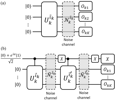
Figure 5: Noise model for the analysis in type (iv). (a) In the circuit to calculate the diagonal element $M_{k}^{\vec{i}_{k},\vec{i}_{k}}(S_{k}^{\vec{i}_{k},\vec{i}_{k}})$, we consider the noise model where the global depolarizing channel $\mathcal{N}_{k}^{\vec{i}_{k}}$ acts just after the unitary gate $U_{k}^{\vec{i}_{k}}$. (b) In the circuit to calculate the off-diagonal element $M_{k}^{\vec{i}_{k},\vec{i}^{\prime}_{k}}(S_{k}^{\vec{i}_{k},\vec{i}^{\prime}_{k}})$, we consider the noise model where the global depolarizing channel $\widehat{\mathcal{N}}_{k}^{\vec{i}_{k}}$ and $\widehat{\mathcal{N}}_{k}^{\vec{i}^{\prime}_{k}}$ act just after the controlled-$U_{k}^{\vec{i}_{k}}$ gate and the controlled-${U}_{k}^{\vec{i}^{\prime}_{k}}$ gate, respectively.

Then, by simple calculations, the noisy Hermitian operators $\tilde{M}_{k}$ and $\tilde{S}_{k}$ can be represented as $\tilde{M}_{k}^{\vec{i}_{k},\vec{i}^{\prime}_{k}}=r_{k}^{\vec{i}_{k},\vec{i}^{\prime}_{k}}M_{k}^{\vec{i}_{k},\vec{i}^{\prime}_{k}}$ and $\tilde{S}_{k}^{\vec{i}_{k},\vec{i}^{\prime}_{k}}=s_{k}^{\vec{i}_{k},\vec{i}^{\prime}_{k}}S_{k}^{\vec{i}_{k},\vec{i}^{\prime}_{k}}$ where

$$r_{k}^{\vec{i}_{k},\vec{i}^{\prime}_{k}}=\begin{cases}1-p_{\,\vec{i}_{k}},&\vec{i}_{k}=\vec{i}^{\prime}_{k},\\ (1-q_{\,\vec{i}_{k}})(1-q_{\,\vec{i}^{\prime}_{k}}),&\vec{i}_{k}\neq\vec{i}^{\prime}_{k},\end{cases}$$ (57)

and

$$s_{k}^{\vec{i}_{k},\vec{i}^{\prime}_{k}}=\begin{cases}1,&\vec{i}_{k}=\vec{i}^{\prime}_{k},\\ (1-q_{\,\vec{i}_{k}})(1-q_{\,\vec{i}^{\prime}_{k}}),&\vec{i}_{k}\neq\vec{i}^{\prime}_{k}.\end{cases}$$ (58)

Here, let us define the following functions $\Gamma_{k}(\bullet)$ and $\Lambda_{k}(\bullet)$ working on the arbitrary matrix with the same size as the $M_{k}^{(4)}$ and $S_{k}^{(4)}$, i.e.

$$\Gamma_{k}\left(\sum_{\vec{i}_{k},\vec{i}^{\prime}_{k}}e^{\vec{i}_{k},\vec{i}^{\prime}_{k}}\ket{\vec{i}_{k}}\bra{\vec{i}^{\prime}_{k}}\right):=\sum_{\vec{i}_{k},\vec{i}^{\prime}_{k}}r_{k}^{\vec{i}_{k},\vec{i}^{\prime}_{k}}e^{\vec{i}_{k},\vec{i}^{\prime}_{k}}\ket{\vec{i}_{k}}\bra{\vec{i}^{\prime}_{k}},$$ (59)

and

$$\Lambda_{k}\left(\sum_{\vec{i}_{k},\vec{i}^{\prime}_{k}}e^{\vec{i}_{k},\vec{i}^{\prime}_{k}}\ket{\vec{i}_{k}}\bra{\vec{i}^{\prime}_{k}}\right):=\sum_{\vec{i}_{k},\vec{i}^{\prime}_{k}}s_{k}^{\vec{i}_{k},\vec{i}^{\prime}_{k}}e^{\vec{i}_{k},\vec{i}^{\prime}_{k}}\ket{\vec{i}_{k}}\bra{\vec{i}^{\prime}_{k}},$$ (60)

where $e^{\vec{i}_{k},\vec{i}^{\prime}_{k}}$ are arbitrary complex numbers for all $\vec{i}_{k}$ and $\vec{i}^{\prime}_{k}$. Note that the functions $\Gamma_{k}$ and $\Lambda_{k}$ transform the operator $M_{k}^{(4)}$ and $S_{k}^{(4)}$ into noisy ones $\tilde{M}_{k}^{(4)}=\Gamma_{k}(M_{k}^{(4)})$ and $\tilde{S}_{k}^{(4)}=\Lambda_{k}(S_{k}^{(4)})$, respectively. Introducing $\Gamma_{k}$ and $\Lambda_{k}~{}(k=1,...,N)$ into Eq. (38), we have

$$\begin{split}\braket{\tilde{O}}_{\rho_{\rm HT}^{(4)}}&=\frac{\mathrm{Tr}[\,\bigotimes_{k=1}^{N}\Gamma_{k}(M_{k}^{(4)})~{}\rho~{}]}{\,\mathrm{Tr}[\,\bigotimes_{k=1}^{N}\Lambda_{k}(S_{k}^{(4)})~{}\rho~{}]}\\ &=\mathrm{Tr}\left[O\cdot\frac{(\bigotimes_{k=1}^{N}A_{k}^{(4)})\bigotimes_{k=1}^{N}\Gamma_{k}(\rho)(\bigotimes_{k=1}^{N}A_{k}^{(4)})^{\dagger}}{(\bigotimes_{k=1}^{N}A_{k}^{(4)})\bigotimes_{k=1}^{N}\Lambda_{k}(\rho)(\bigotimes_{k=1}^{N}A_{k}^{(4)})^{\dagger}}\right].\end{split}$$ (61)

Regarding the component separated from the observable $O$ as effective density operator $\tilde{\rho}_{\rm HT}^{(4)}$, we obtain

$$\tilde{\rho}_{\rm HT}^{(4)}=\frac{(\bigotimes_{k=1}^{N}A_{k}^{(4)})\bigotimes_{k=1}^{N}\Gamma_{k}(\rho)(\bigotimes_{k=1}^{N}A_{k}^{(4)})^{\dagger}}{(\bigotimes_{k=1}^{N}A_{k}^{(4)})\bigotimes_{k=1}^{N}\Lambda_{k}(\rho)(\bigotimes_{k=1}^{N}A_{k}^{(4)})^{\dagger}}.$$ (62)

Since $\otimes_{k=1}^{N}\Gamma_{k}(\rho)$ is not always a positive-semidefinite operator in general, we arrive at the conclusion that $\tilde{\rho}_{\rm HT}$ could have negative eigenvalues.

IV.6 Classical case

Let us consider the case where $\xi_{k}=\mathrm{c}$ for all $k$. Given that errors in classical computations are sufficiently small and negligible, the contracted operators $\tilde{M}_{k}^{(\mathrm{c})}$ and $\tilde{S}_{k}^{(\mathrm{c})}$ can be represented as $\tilde{M}^{(\mathrm{c})}_{k}=M^{(\mathrm{c})}_{k}={A_{k}^{(\mathrm{c})}}^{\dagger}O_{k}A^{(\mathrm{c})}_{k}$ and $\tilde{S}^{(\mathrm{c})}_{k}=S^{(\mathrm{c})}_{k}={A_{k}^{(\mathrm{c})}}^{\dagger}A^{(\mathrm{c})}_{k}$. Thus, the following equations clearly hold:

$$\begin{split}\mathrm{Tr}[\,\tilde{M}_{k}^{(\mathrm{c})}\bullet\,]&=\mathrm{Tr}[\,O_{k}\,\tilde{\mathcal{A}}^{(c)}_{k}(\bullet)\,],\\ \mathrm{Tr}[\,\tilde{S}_{k}^{(\mathrm{c})}\bullet\,]&=\mathrm{Tr}[\,\tilde{\mathcal{A}}^{(\mathrm{c})}_{k}(\bullet)\,],\end{split}$$ (63)

where we defined $\tilde{\mathcal{A}}^{(\mathrm{c})}_{k}(\bullet)=A^{(\mathrm{c})}_{k}\bullet{A_{k}^{(\mathrm{c})}}^{\dagger}$. Hence, we can easily obtain

$$\tilde{\rho}_{\rm HT}^{(\mathrm{c})}=\frac{(\bigotimes_{k=1}^{N}A_{k}^{(\mathrm{c})})\,\rho\,(\bigotimes_{k=1}^{N}A_{k}^{(\mathrm{c})})^{\dagger}}{\mathrm{Tr}[(\bigotimes_{k=1}^{N}A_{k}^{(\mathrm{c})})\,\rho\,(\bigotimes_{k=1}^{N}A_{k}^{(\mathrm{c})})^{\dagger}]}.$$ (64)

Since $\rho$ is a density operator, $\tilde{\rho}_{\rm HT}^{(\mathrm{c})}$ is obviously a density operator.

IV.7 Quantum-classical mixed-type HTTN state preparations with multiple layers

In the preceding discussions, we have investigated a noisy effective HTTN state $\tilde{\rho}_{\rm HT}$ with two layers. In those analyses, we have considered all subsystems to share the same type of state preparation. Here, extending the previous discussion, let us consider the effect of physical noise on a quantum-classical mixed-type HTTN state with $L$ layers. To begin with, we consider the density matrix representation of a noiseless tree tensor state:

$$\rho_{\rm HT}=\frac{\mathcal{A}_{L}\circ\mathcal{A}_{L-1}\circ\cdots\mathcal{A}_{2}(\rho)}{\mathrm{Tr}[\mathcal{A}_{L}\circ\mathcal{A}_{L-1}\circ\cdots\mathcal{A}_{2}(\rho)]},$$ (65)

where $\rho$ is a parent classical or quantum tensor. In Eq. (65), we define the $l$-th layer’s operator $\mathcal{A}_{l}(\bullet)$ for $l=2,...,L$ as

$$\mathcal{A}_{l}(\bullet)=\mathcal{A}_{l,1}^{(\xi_{l,1})}\otimes\mathcal{A}_{l,2}^{(\xi_{l,2})}\otimes\cdots\otimes\mathcal{A}_{l,N_{l}}^{(\xi_{l,N_{l}})}(\bullet),$$ (66)

where $\mathcal{A}_{l,\mu}^{(\xi_{l,\mu})}(\bullet)$ is the $l$-th layer’s $\mu$-th operator defined as $\mathcal{A}_{l,\mu}^{(\xi_{l,\mu})}(\bullet)=A_{l,\mu}^{(\xi_{l,\mu})}\bullet{A_{l,\mu}^{(\xi_{l,\mu})}}^{\dagger}$ with $A_{l,\mu}^{(\xi_{l,\mu})}=\sum_{\vec{i}_{l,\mu}}\ket{\psi_{l,\mu}^{\vec{i}_{l,\mu}}}\bra{\vec{i}_{l,\mu}}$ for $\mu=1,...,N_{l}$. The graphical description of the state $\rho_{\rm HT}$ is shown in Fig. 6. Hereafter, we only consider types (i)-(iii) and classical tensor preparations because type (iv) may induce unphysicality.

The assumptions of physical noise in the computation for the main system and each subsystem follow the previous discussions: the physical noise in quantum computation converts an ideal unitary channel to a noisy one. Additionally, for simplicity, we consider the case where the observable $O$ is written as $O=O_{L,1}\otimes\cdots\otimes O_{L,N_{L}}$, and note that the same line of discussion holds for observables without tensor product structure.

Figure 6: The graphical diagrams of the quantum-classical mixed-type HTTN state $\rho_{\rm HT}$ with $L$ layers and the observable $O$. The ansatz is composed of the parent classical or quantum tensor $\rho$, and the $l$-th layer’s $\mu$-th operators $\mathcal{A}_{l,\mu}^{(\xi_{l,\mu})}$ where $\xi_{l,\mu}$ takes four different values: $\xi_{l,\mu}=1$(orange vertices), $2$(green vertices), $3$(blue vertices), and $\mathrm{c}$ (yellow vertices). In actual calculations, the contractions are performed sequentially from $\tilde{M}_{L}$ down to $\tilde{M}_{2}$, and at each contraction step, physical noise propagates to the upper layer.

In the calculations of this setting, we sequentially construct the contracted operators $\tilde{M}_{l}$ and $\tilde{S}_{l}$ from the $L$-th layer to the 2nd layer, i.e., $\tilde{M}_{L}\rightarrow\tilde{M}_{L-1}\rightarrow\cdots\rightarrow\tilde{M}_{2}$ and $\tilde{S}_{L}\rightarrow\tilde{S}_{L-1}\rightarrow\cdots\rightarrow\tilde{S}_{2}$. Using the lastly obtained operators $\tilde{M}_{2}$, $\tilde{S}_{2}$, and $\rho$, we obtain the noisy expectation value $\braket{\tilde{O}}_{\rho_{\rm HT}}$ as

$$\braket{\tilde{O}}_{\rho_{\rm HT}}=\frac{\mathrm{Tr}[\,\tilde{M}_{2}\,\rho\,]}{\mathrm{Tr}[\,\tilde{S}_{2}\,\rho\,]}.$$ (67)

Our objective is to explicitly express the noisy effective state $\tilde{\rho}_{\rm HT}$ defined as $\braket{\tilde{O}}_{\rho_{\rm HT}}=\braket{O}_{\tilde{\rho}_{\rm HT}}$. To this end, from Eqs. (41), (46), (51), and (63), we make the following equations:

$$\mathrm{Tr}[\,\tilde{M}_{l^{\prime}}\bullet\,] =\mathrm{Tr}[\,\tilde{M}_{l^{\prime}+1}\,\tilde{\mathcal{A}}_{l^{\prime}}(\bullet)\,],$$ (68)

$$\mathrm{Tr}[\,\tilde{S}_{l^{\prime}}\bullet\,] =\mathrm{Tr}[\,\tilde{S}_{l^{\prime}+1}\,\tilde{\mathcal{A}}_{l^{\prime}}(\bullet)\,],$$ (69)

for $l^{\prime}=2,...,L-1$, and

$$\mathrm{Tr}[\,\tilde{M}_{L}\bullet\,] =\mathrm{Tr}[\,O\,\tilde{\mathcal{A}}_{L}(\bullet)\,],$$ (70)

$$\mathrm{Tr}[\,\tilde{S}_{L}\bullet\,] =\mathrm{Tr}[\,\tilde{\mathcal{A}}_{L}(\bullet)\,].$$ (71)

By iteratively employing Eqs. (68)–(71) on Eq. (67), we obtain

$$\begin{split}\braket{\tilde{O}}_{\rho_{\rm HT}}&=\frac{\mathrm{Tr}[\,\tilde{M}_{2}\,\rho\,]}{{\mathrm{Tr}[\,\tilde{S}_{2}\,\rho\,]}}\\ &=\frac{\mathrm{Tr}[\,\tilde{M}_{3}\,\tilde{\mathcal{A}}_{2}(\rho)\,]}{\mathrm{Tr}[\,\tilde{S}_{3}\,\tilde{\mathcal{A}}_{2}(\rho)\,]}\\ &=\cdots\\ &=\frac{\mathrm{Tr}\Bigl{[}\,O\,\Bigl{(}\tilde{\mathcal{A}}_{L}\circ\tilde{\mathcal{A}}_{L-1}\circ\cdots\circ\tilde{\mathcal{A}}_{2}(\rho)\Bigr{)}\,\Bigr{]}}{\mathrm{Tr}\Bigl{[}\,\tilde{\mathcal{A}}_{L}\circ\tilde{\mathcal{A}}_{L-1}\circ\cdots\circ\tilde{\mathcal{A}}_{2}(\rho)\,\Bigr{]}}.\end{split}$$ (72)

Thus, the effective state can be expressed as

$$\tilde{\rho}_{\rm HT}=\frac{\tilde{\mathcal{A}}_{L}\circ\tilde{\mathcal{A}}_{L-1}\circ\cdots\circ\tilde{\mathcal{A}}_{2}(\rho)}{\mathrm{Tr}\Bigl{[}\tilde{\mathcal{A}}_{L}\circ\tilde{\mathcal{A}}_{L-1}\circ\cdots\circ\tilde{\mathcal{A}}_{2}(\rho)\Bigr{]}}.$$ (73)

Here, since the operator $\rho$ is quantum state by definition and the mappings $\tilde{\mathcal{A}}_{l}(\bullet)$($l=2,...,L$) defined in Eq. (66) are CP maps (see Appendix B), the numerator of Eq. (73) is thereby a positive semidefinite operator. Taking into account the normalization term in Eq. (73), $\tilde{\rho}_{\rm HT}$ is a density operator.

IV.8 Application to previously proposed methods

Here, we apply the expansion operator method to Deep VQE and the entangling forging method. Then, we see the explicit density matrix representation and discuss the physicality of the HTN state under the effect of hardware noise.

IV.8.1 Deep VQE

In Sec. III.1, we have captured the Deep VQE algorithm in the framework of HTTNs. Here, using the operator representation of HTTNs, we express Deep VQE ansatz $\rho_{\rm DV}$ corresponding to Eq. (26) as

$$\rho_{\rm DV}=\mathcal{A}_{3}\circ\mathcal{A}_{2}(\ket{\phi}\bra{\phi}),$$ (74)

where $\ket{\phi}\bra{\phi}$ is a parent quantum tensor, and $\mathcal{A}_{2}$ and $\mathcal{A}_{3}$ are the 2nd and 3rd layer’s operators defined as

$$\mathcal{A}_{2}(\bullet) =\mathcal{A}_{2,1}^{(\xi_{2,1})}\otimes...\otimes\mathcal{A}_{2,N}^{(\xi_{2,N})}(\bullet),$$ (75)

$$\mathcal{A}_{3}(\bullet) =\mathcal{A}_{3,1}^{(\xi_{3,N})}\otimes...\otimes\mathcal{A}_{3,N}^{(\xi_{3,N})}(\bullet).$$ (76)

$\mathcal{A}_{2,s}^{(\xi_{2,s})}(\bullet)=A_{2,s}^{(\xi_{2,s})}\bullet{A_{2,s}^{(\xi_{2,s})}}^{\dagger}$ are the 2nd layer’s $s$-th operators where $A_{2,s}^{(\xi_{2,s})}$ is defined as

$$A_{2,s}^{(\xi_{2,s})}=\sum_{\vec{i}_{s}\in\{0,1\}^{\kappa_{s}}}\ket{\psi_{2,s}^{\vec{i}_{s}}}\bra{\vec{i}_{s}},$$ (77)

and $\ket{\psi_{2,s}^{\vec{i}_{s}}}=\sum_{\vec{j}_{s}\in\{0,1\}^{\kappa_{s}}}P^{\vec{i}_{s},\vec{j}_{s}}_{s}\ket{\vec{j}_{s}}$. Note that $P^{\vec{i}_{s},\vec{j}_{s}}_{s}$ corresponds to $P^{mm^{\prime}}_{s}$ in Eq. (15). Since each element of $\ket{\psi_{2,s}^{\vec{i}_{s}}}$ is stored in a classical register, the operator $A_{2,s}^{(\xi_{2,s})}$ is a classical tensor, i.e., $\xi_{2,s}=\mathrm{c}$ for all $s$. $\mathcal{A}_{3,s}^{(\xi_{3,s})}(\bullet)=A_{3,s}^{(\xi_{3,s})}\bullet{A_{3,s}^{(\xi_{3,s})}}^{\dagger}$ is the 3rd layer’s $s$-th operator where

$$A_{3,s}^{(\xi_{3,s})}=\sum_{\vec{j}_{s}\in\{0,1\}^{\kappa_{s}}}\ket{\psi_{3,s}^{\vec{j}_{s}}}\bra{\vec{j}_{s}},$$ (78)

and

$$\ket{\psi_{3,s}^{\vec{j}_{s}}}=\begin{cases}D^{\vec{j}_{s}}_{s}\ket{\psi_{s}^{\mathrm{G}}},&(\vec{j}_{s})_{(10)}\leq K_{s}-1,\\ \vec{0},&(\vec{j}_{s})_{(10)}\geq K_{s}.\end{cases}$$ (79)

When setting the operator $D^{m}_{s}$ as the Pauli operators, it is clear that $\xi_{3,s}=1$ for all $s$. Alternatively, when we adopt the general local excitation operator $D^{\vec{j}_{s}}_{s}$ as $W^{\vec{j}_{s}}_{s}$, the computational process in Eq. (18) remains the same as type (iii) in Sec. II.3. Thus, without loss of generality, we can consider $\xi_{3,s}=1$ for all $s$.

Now, we consider the effect of physical noise. From the discussions in Sec. IV.4 and  IV.6, $\tilde{\mathcal{A}}_{2}$ and $\tilde{\mathcal{A}}_{3}$ are CP maps, so the effective noisy state $\tilde{\rho}_{\rm DV}=\tilde{\mathcal{A}}_{3}\circ\tilde{\mathcal{A}}_{2}(\rho)$ is a positive semidefinite operator. However, the operator $\mathcal{A}_{2}$, playing a role in normalizing $\rho_{\rm DV}$, is composed of $P^{\vec{i}_{s},\vec{j}_{s}}_{s}$, which is also susceptible to physical noise, $\mathrm{Tr}[\tilde{\rho}_{\rm DV}]=1$ may not be maintained.

To address this problem, one possible solution is to modify the ansatz in Eq. (74) as follows:

$$\rho_{\rm DV2}=\frac{\mathcal{A}_{3}(\ket{\phi}\bra{\phi})}{\mathrm{Tr}[\mathcal{A}_{3}(\ket{\phi}\bra{\phi})]},$$ (80)

where the definition of $\mathcal{A}_{3}$ follows Eq. (76),(78), and (79). The denominator in Eq. (80) is derived from the list of inner products $\{\braket{\psi_{s}^{\vec{i}_{s}}}{\psi_{s}^{\vec{j}_{s}}}\}$, which is used to construct $\mathcal{A}_{2}$ in Eq. (74). As $\rho_{\rm DV2}$ is composed solely of type (iii) operators, it follows from the discussion in Sec. IV.7 that the noisy state $\tilde{\rho}_{\rm DV2}$ can maintain the properties of the density operator.

IV.8.2 Entanglement forging

Following the notation in Sec. III.2, the operator representation $\rho_{\rm EF}$ of entanglement forging ansatz is represented as

$$\rho_{\rm EF}=\mathcal{A}_{2}(\ket{\phi}\bra{\phi}),$$ (81)

where $\ket{\phi}$ is a vector whose elements are derived from the Schmidt coefficients, and stored in a classical register. The operator $\mathcal{A}_{2}$ is defined as follows:

$$\mathcal{A}_{2}(\bullet)=\mathcal{A}_{2,s}^{(\xi_{2,1})}\otimes\mathcal{A}_{2,s}^{(\xi_{2,2})}(\bullet).$$ (82)

$\mathcal{A}_{2,s}^{(\xi_{2,s})}(\bullet)=A_{2,s}^{(\xi_{2,s})}\bullet{A_{2,s}^{(\xi_{2,s})}}^{\dagger}$ is the 2nd layer’s $s$-th operator where $A_{2,s}^{(\xi_{2,s})}$ is defined as

$$A_{2,s}^{(\xi_{2,s})}=\sum_{\vec{i}_{s}\in\{0,1\}^{N}}\ket{\psi^{\vec{i}_{s}}_{2,s}}\bra{\vec{i}_{s}},$$ (83)

and $\ket{\psi^{\vec{i}_{s}}_{2,s}}=V_{s}\ket{\vec{i}_{s}}$. From the structure of the state $\ket{\psi^{\vec{i}_{s}}_{2,s}}$, we see that $\xi_{s}=1$ for $s=1,2$.

Here, we made the same assumptions made so far, where the 1st and 2nd subsystems’s unitary channel $\mathcal{U}_{1}(\bullet)=U_{1}\bullet U_{1}^{\dagger}$ and $\mathcal{U}_{2}(\bullet)=U_{2}\bullet U_{2}^{\dagger}$ are transformed into noisy channel $\mathcal{W}_{1}(\bullet)$ and $\mathcal{W}_{2}(\bullet)$, respectively. Then, as $\rho_{\rm EF}$ is constructed from type (i) operators, the analysis in Sec. IV shows that noisy state $\tilde{\rho}_{\rm EF}=\tilde{\mathcal{A}}_{2}(\ket{\phi}\bra{\phi})$ preserves its property as a density operator.

V Analysis of noise propagation for specific noise models

Here, we further delve into the expansion operator by specifying the noise model to the global depolarizing model for each quantum tensor. Note that global depolarizing noise has been shown to be a good approximation for error mitigation [41, 42, 43, 44]. We show that the expectation value of observables exponentially vanishes with the number of quantum tensors.

Here, we assume that the global depolarizing channel acts just after the unitary channel in Fig. 2. In this case, the expansion operators $\tilde{\mathcal{A}}^{(\xi_{k})}_{k}(\xi_{k}=1,2,3)$ for a noisy quantum tensor can be represented as:

$$\tilde{\mathcal{A}}^{(\xi_{k})}_{k}(\bullet)=(1-\varepsilon_{k})\mathcal{A}^{(\xi_{k})}_{k}(\bullet)+\varepsilon_{k}\mathcal{K}^{(\xi_{k})}_{k}(\bullet),$$ (84)

where $\varepsilon_{k}$ are noise rates, $\mathcal{A}^{(\xi_{k})}_{k}$ is the noiseless expansion operator, and

$$\mathcal{K}^{(\xi_{k})}_{k}(\bullet)=\begin{cases}\frac{I^{\otimes K_{k}}}{2^{K_{k}}},&\xi_{k}=1,\\ \mathrm{Tr}(\bullet)\frac{I^{\otimes K_{k}}}{2^{K_{k}}},&\xi_{k}=2,\\ \mathcal{P}_{k}^{(3)\dagger}\bigl{\{}(\bullet)\otimes\frac{I^{\otimes K_{k}}}{2^{K_{k}}}\bigr{\}}\mathcal{P}_{k}^{(3)},&\xi_{k}=3.\end{cases}$$ (85)

By assuming that the HTN state consists only of noisy quantum tensors and that $\varepsilon_{k}=\varepsilon$ for simplicity, we obtain

$$\bigcirc_{k=2}^{N_{\mathrm{tot}}}\tilde{\mathcal{A}}^{(\xi_{k})}_{k}(\rho) =(1-\varepsilon)^{N_{\mathrm{tot}}-1}\bigcirc_{k=2}^{N_{\mathrm{tot}}}\mathcal{A}^{(\xi_{k})}_{k}(\rho)$$ (86)

$$+\sum_{m=1}^{N_{\mathrm{tot}}-1}p(N_{\mathrm{tot}}-1,m,\varepsilon)\mathcal{B}_{m},$$

where $p(N_{\mathrm{tot}}-1,m,\varepsilon)=\binom{N_{\mathrm{tot}}-1}{m}(1-\varepsilon)^{N_{\mathrm{tot}}-m-1}\varepsilon^{m}$ is the binomial distribution, and $\mathcal{B}_{m}$ is the process in which the error $\mathcal{K}_{k}^{(\xi_{k})}$ occurs $m$ times. Here, $\bigcirc_{k=1}^{N}\mathcal{E}_{k}=\mathcal{E}_{N}\circ\mathcal{E}_{N-1}\circ...\circ\mathcal{E}_{1}$ for a quantum process $\mathcal{E}_{k}~{}(k=1,2,...,N)$. The process $\mathcal{B}_{m}$ renders the HTN states highly mixed, which makes expectation values of non-local Pauli observables negligible. Then we can regard $\bigcirc_{k=2}^{N_{\mathrm{tot}}}\tilde{\mathcal{A}}^{(\xi_{k})}_{k}(\rho)\sim(1-\varepsilon)^{N_{\mathrm{tot}}-1}\bigcirc_{k=2}^{N_{\mathrm{tot}}}\mathcal{A}^{(\xi_{k})}_{k}(\rho)$.

Considering the $L$-layer TTNs consisting of noisy $N$-rank quantum tensors, since the total number of the contracted quantum tensor is $N_{\rm tot}=1+N+N^{2}+...+N^{L-1}=\frac{1-N^{L}}{1-N}$, we have

$$\braket{O}_{\rm noisy}\sim(1-\varepsilon)^{\frac{1-N^{L}}{1-N}}\braket{O}_{\rm EF}.$$ (87)

We numerically verify Eq. (87) by simulating a $L$-layer TTN comprising of noisy rank-$N$ tensors $\rho_{\vec{i},\vec{i}^{\prime}}$ for $\vec{i}=(i_{1},i_{2},...,i_{N}),~{}i_{k}\in\{0,1\}$ for $O=Z^{\otimes N^{L}}$ with the type (i) state preparation. Each tensor is generated by a two-layer hardware-efficient ansatz shown in Fig. 7, accompanied by the global depolarizing noise. For efficiently simulating noisy TTNs, once we obtain a contracted matrix $\tilde{M}$ in some layer, we use $\tilde{M}^{\otimes N}$ for the contraction in the next layer.

We then show the ratio between the noise-free and the noisy value $r_{L}(\varepsilon)=\braket{O}_{\rm noisy}/\braket{O}_{\rm EF}$ for $L=4,5,6$ with $N=10$ in Fig. 8. In all the cases, we can see

$$\tilde{r}_{L}(\varepsilon)=(1-\varepsilon)^{\frac{1-N^{L}}{1-N}}$$ (88)

exactly coincides with the numerical results, which indicates Eq. (87) is a very good approximation.

When we can characterize the value of $\varepsilon$, division of $\braket{O}_{\rm noisy}$ by $\tilde{r}_{L}(\varepsilon)$ yields:

$$\braket{O}_{\rm QEM}=\braket{O}_{\rm noisy}/\tilde{r}_{L}(\varepsilon),$$ (89)

which effectively works as quantum error mitigation [45, 46, 8, 47]. However, for the variance of the error mitigated result $\braket{O}_{\rm QEM}$, we obtain

$$\mathrm{Var}[\braket{O}_{\rm QEM}]=\tilde{r}_{L}(\varepsilon)^{2}\mathrm{Var}[\braket{O}_{\rm noisy}],$$ (90)

resulting in the necessity to have $\tilde{r}_{L}(\varepsilon)^{2}$ times more samples to achieve the same accuracy as the error-free case.

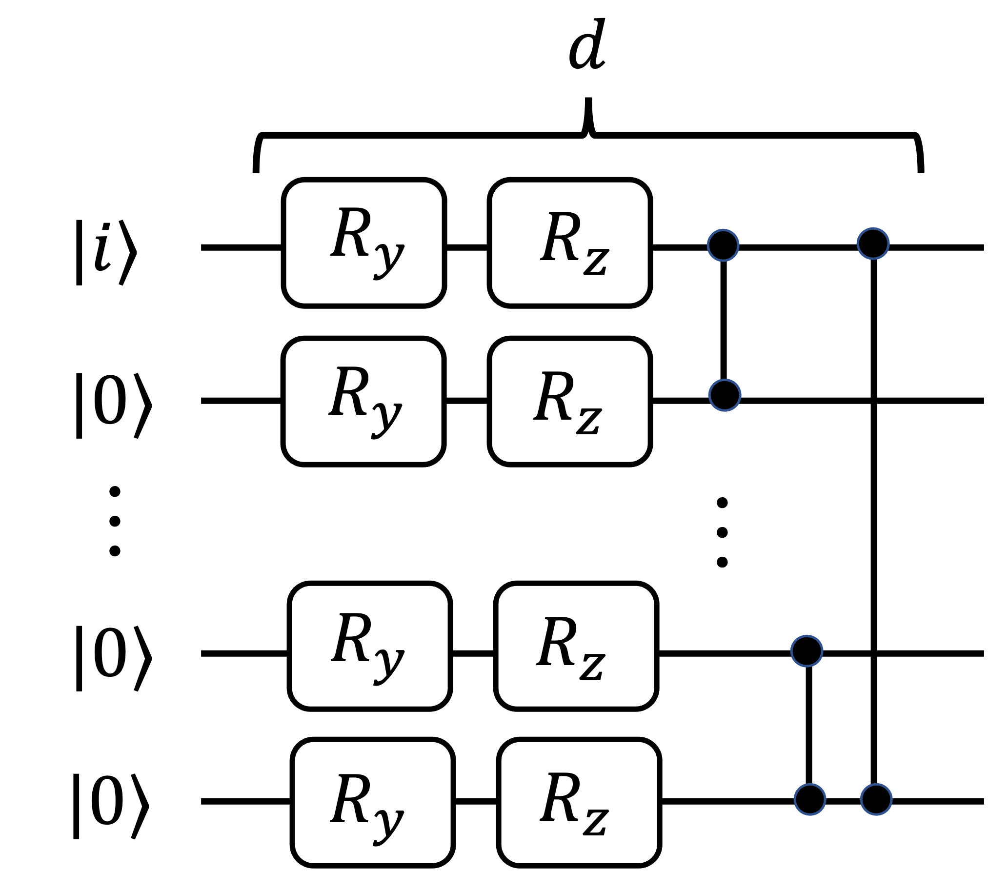
Figure 7: Hardware-efficient ansatz used in numerical simulations. Because we simulate type (i) contraction, we set the first register to $i=0,1$. To avoid extremely small computation results that induce numerical errors, we restrict variational rotation angles to the range of $[-\pi/10^{3},\pi/10^{3}]$. We set $d=2$.

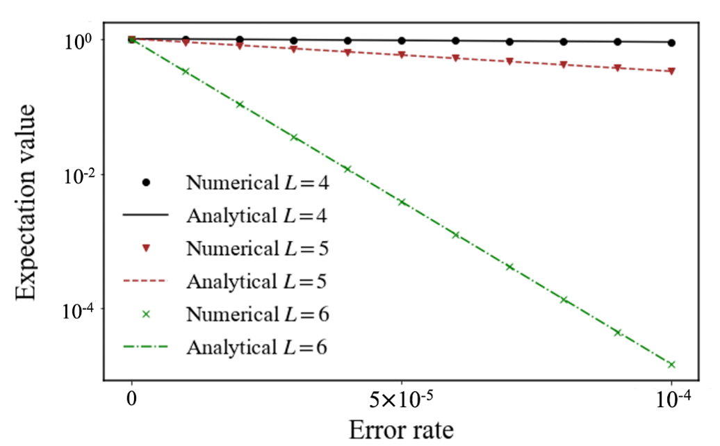
Figure 8: The ratio of the noisy and the noise-free computation results $r(\varepsilon)$ versus the error rate $\varepsilon$. The numerically simulated result $r(\varepsilon)$ and its approximation $\tilde{r}(\varepsilon)$ in Eq. (88) exactly coincide. We simulate $N=10$.

These discussions indicate that, although the simulatable scale of the quantum systems can be significantly expanded, we need to have exponential resources with the number of contracted quantum tensors. To avoid this problem, we must take the following strategies: (1). adjusting the number of classical and quantum tensors in accordance with the magnitude of the error; or (2). suppressing the error rate itself with error-suppression techniques such as quantum error correction [48, 49] and dynamical decoupling [50]. In terms of (1), replacing the quantum tensors with the classical tensors in the $L$-layer, for example, yields $\braket{O^{\prime}}_{\rm noisy}\sim(1-\varepsilon)^{\frac{1-N^{L-1}}{1-N}}\braket{O}_{\rm EF}\sim(1-\varepsilon)^{-N^{L-1}}\braket{O}_{\rm noisy}$, and the problem of exponential decay of the observable is mitigated.

VI Conclusions and Discussions

In this paper, we first reviewed the hybrid tensor network (HTN) framework and discussed the related methods, i.e., the Deep VQE and entanglement forging under the language of HTN. Then, whereas these methods are formulated for pure states, the quantum states should be described with the density matrices due to the effect of physical noise in actual experiments. Therefore, we introduced the density matrix representation for HTNs by introducing the expansion operator and discussed the HTN states’ physicality by considering each contraction method case. We found that as long as we use type (i)-(iii) state preparation, the HTN state is physical, while type (iv) may induce unphysical states. We also revealed that the exponential decay of the computation results occurs with the number of contracted quantum tensors in the tree network.

While we mainly analyzed the expectation values, some algorithms use transition amplitudes in the HTN framework, e.g., quantum-inspired Monte-Carlo simulations [20]; therefore, we cannot directly apply our arguments to this case, although the exponential decay of the measured values with the number of quantum tensors is likely to be observed. Also, based on the results of the explicit formulas for HTN states under noise, it may be interesting to apply quantum error mitigation (QEM), e.g., probabilistic error cancellation with finite noise characterization errors [51], to HTN states and see the resulting effective quantum states and its physicality. Finally, although we derived the exponential decay of the observables for tree tensor networks with noisy quantum states and the exponential growth of the variance of the error-mitigated observable for a specific strategy in Eq. (89), the application of information-theoretic analysis of QEM [52, 53, 41, 54] for HTN states may be useful to verify the efficiency of this QEM protocol.

VII Acknowledgments

This project is supported by Moonshot R&D, JST, Grant No. JPMJMS2061; MEXT Q-LEAP Grant No. JPMXS0120319794, and No.  JPMXS0118068682 and PRESTO, JST, Grant No.  JPMJPR2114, No.  JPMJPR1916, and JST CREST Grant No. JPMJCR23I4, Japan. We would like to thank the summer school on ”A novel numerical approach to quantum field theories” at the Yukawa Institute for Theoretical Physics (YITP-W-22-13) for providing us with the opportunity to deepen our ideas. We thank Shu Kanno, Nobuyuki Yoshioka and Hideaki Hakoshima for useful discussions.

Appendix A Equivalence between Eq. (34) and Eq. (35)

The aim of this section is to introduce HTN representation based on the operator $A=\sum_{\vec{i}}\ket{\psi^{\vec{i}}}\bra{\vec{i}}$ used in the main text and rewrite Eq. (34) to the mathematically equivalent expression as shown in Eq. (35). To begin with, let us review the structure of the 2-layer HTTN state $\ket{\psi_{\rm HT}}$ in Eq. (34):

$$\ket{\psi_{\rm HT}}=\frac{1}{C}\sum_{\vec{i}_{1},...,\vec{i}_{N}}\phi_{\vec{i}_{1},...,\vec{i}_{N}}\ket{\psi_{1}^{\vec{i}_{1}}}\otimes\cdots\otimes\ket{\psi_{N}^{\vec{i}_{N}}},$$ (91)

where $\vec{i}_{k}\in\{0,1\}^{\tau_{k}}(k=1,...,N)$ is a classical bit string, $\phi_{\vec{i}_{1},...,\vec{i}_{N}}=\braket{\vec{i}_{1},...,\vec{i}_{N}}{\phi}$ is the probability amplitude of a $(\sum_{k=1}^{N}\tau_{k})$-qubit system, $\ket{\phi_{k}^{\vec{i}_{k}}}(k=1,...,N)$ is a $K_{k}$-qubit state of the $k$-th subsystem, $C$ be a normalization constant, and $\ket{\psi_{\rm HT}}$ is a $\kappa$-qubit state where $\kappa=\sum_{k}K_{k}$.

Focusing on the the non-local tensor $\phi_{\vec{i}_{1},...,\vec{i}_{N}}$ and local state $\ket{\psi_{k}^{\vec{i}_{k}}}$ in subsystem $k$, the following connecting relation exists:

$$\sum_{\vec{i}_{k}}\phi_{\vec{i}_{k},...}\ket{\psi^{\vec{i}_{k}}_{k}}=\sum_{\vec{i}_{k}}\braket{\vec{i}_{k}}{\phi}\ket{\psi_{k}^{\vec{i}_{k}}}.$$ (92)

In this expression, the index $\vec{i}_{k}$ of the non-local tensor $\phi_{\vec{i}_{k},...}$ is linked with the labeled state $\ket{\psi_{k}^{\vec{i}_{k}}}$ from the set of state $\{\ket{\psi_{k}^{\vec{i}_{k}}}\}_{\vec{i}_{k}}$. Here, we can rewrite Eq. (92) as follows:

$$\sum_{\vec{i}_{k}}\phi_{\vec{i}_{k},...}\ket{\psi^{\vec{i}_{k}}_{k}}=A_{k}^{(\xi_{k})}\ket{\phi}.$$ (93)

We have defined $A_{k}^{(\xi_{k})}:=\sum_{\vec{i}_{k}}\ket{\psi^{\vec{i}_{k}}_{k}}\bra{\vec{i}_{k}}$ where the upper subscript $\xi_{k}\in\{1,2,3,4,\mathrm{c}\}$ represents the different way of preparing the set of state $\{\ket{\psi_{k}^{\vec{i}_{k}}}\}_{\vec{i}_{k}}$, e.g, $\{\ket{\psi_{k}^{\vec{i}_{k}}}\}_{\vec{i}_{k}}=\{U_{k}\ket{\vec{i}_{k}}\ket{\vec{0}}\}_{\vec{i}_{k}}$ for $\xi_{k}=1$, and $\{\ket{\psi_{k}^{\vec{i}_{k}}}\}_{\vec{i}_{k}}=\{\mathrm{Tr}[\alpha_{1}^{j_{1},\vec{i}_{k}}...\alpha_{K}^{j_{K}}]\ket{j_{1}...j_{K}}\}_{\vec{i}_{k}}$ for $\xi_{k}=\mathrm{c}$. In this picture, we can see that the operator $A_{k}^{(\xi_{k})}$ extends the size of the quantum state $\ket{\phi}$. By introducing the operators $A_{k}^{(\xi_{k})}(k=1,...,N)$ into Eq. (91), we have

$$\ket{\psi_{\rm HT}}=\frac{1}{C}(A_{1}^{(\xi_{1})}\otimes...\otimes A_{N}^{(\xi_{N})})\ket{\phi}.$$ (94)

Then, representing Eq. (94) in the form of a density matrix, we obtain the following expression as shown in Eq. (35):

$$\rho_{\rm HT}=\frac{(A_{1}^{(\xi_{1})}\otimes...\otimes A_{N}^{(\xi_{N})})\ket{\phi}\bra{\phi}(A_{1}^{(\xi_{1})}\otimes...\otimes A_{N}^{(\xi_{N})})^{\dagger}}{\mathrm{Tr}[(A_{1}^{(\xi_{1})}\otimes...\otimes A_{N}^{(\xi_{N})})\ket{\phi}\bra{\phi}(A_{1}^{(\xi_{1})}\otimes...\otimes A_{N}^{(\xi_{N})})^{\dagger}]}.$$ (95)

Appendix B Datailed calculations to obtain Eq. (41), (46), and (51)

When calculating the expectation value of an observable for the HTTN state $\rho_{\rm HT}$ as in Eq. (35), we sequentially perform contractions between local tensors and Hermitian operators from the lower layers to the upper layers. In each contraction step, for an $K$-qubit observable $O$ and a local operator $A^{(\xi)}=\sum_{\vec{i}\in\{0,1\}^{\tau}}\ket{\psi^{\vec{i}}}\bra{\vec{i}}$ connected to $O$ where $\xi$ indicates the different way to define $\ket{\psi^{\vec{i}}}$, we construct a new Hermitian operator as

$$\begin{split}M^{(\xi)}&=A^{(\xi)\dagger}OA^{(\xi)},\\ S^{(\xi)}&=A^{(\xi)\dagger}A^{(\xi)},\end{split}$$ (96)

by the measurements on a quantum computer ($\xi=1,2,3,4$) or the classical calculations ($\xi=\mathrm{c}$).

In actual calculations, however, the quantum circuits to calculate $M^{(\xi)}$ are susceptible to physical noise, and thus we obtain the noisy Hermitian operator $\tilde{M}^{(\xi)}$. Here, we assume that the unitary channel $\mathcal{U}(\bullet)=U\bullet U^{\dagger}$ in quantum circuits to calculate $M^{(\xi)}$, as shown in Fig. 2, is changed into the noisy one $W(\bullet)$. Then, there exists a linear operator $\tilde{\mathcal{A}}^{(\xi)}(\bullet)$($\xi=1,2,3$) satisfying the following relation for any $2^{K}\times 2^{K}$ complex matrices $X$:

$$\mathrm{Tr}[\,\tilde{M}^{(\xi)}X\,] =\mathrm{Tr}[\,O\,\tilde{\mathcal{A}}^{(\xi)}(X)\,],$$ (97)

$$\mathrm{Tr}[\,\tilde{S}^{(\xi)}X\,] =\mathrm{Tr}[\,\tilde{\mathcal{A}}^{(\xi)}(X)\,].$$ (98)

Since Eq. (98) can be derived by substituting $O=I^{\otimes K}$ into Eq. (97), we mainly prove Eq. (97), and check that $\tilde{\mathcal{A}}^{(\xi)}(\bullet)$ is a completely positve (CP) map for $\xi=1,2,3$. In the following, for the finite-dimensional Hilbert space $\mathcal{H}_{\rm B}$ of a system $\rm B$, let $\mathcal{L}(\mathcal{H}_{\rm B})$ denote the family of linear operators acting on $\mathcal{H}_{\rm B}$.

B.1 Type (i)

In this case, the noisy Hermitian operator $\tilde{M}^{(1)}$ is written as

$$\tilde{M}^{(1)}=\sum_{\vec{i},\vec{i}^{\prime}}\mathrm{Tr}\left[\,O\,\mathcal{W}\left(\ket{\vec{i}^{\prime}}\bra{\vec{i}}\otimes{\ket{\vec{0}}\bra{\vec{0}}}\right)\,\right]\ket{\vec{i}}\bra{\vec{i}^{\prime}}.$$ (99)

Then, we have the following equation for any $2^{K}\times 2^{K}$ complex matrix $X$.

$$\begin{split}\mathrm{Tr}[\tilde{M}^{(1)}X]&=\sum_{\vec{i},\vec{i}^{\prime}}\mathrm{Tr}\left[\,O\,\mathcal{W}\left(\ket{\vec{i}^{\prime}}\bra{\vec{i}}\otimes{\ket{\vec{0}}\bra{\vec{0}}}\right)\,\right]\braket{\vec{i}^{\prime}}{X}{\vec{i}}\\ &=\mathrm{Tr}\biggl{[}\,O\,\mathcal{W}\biggl{(}\sum_{\vec{i},\vec{i}^{\prime}}\braket{\vec{i}^{\prime}}{X}{\vec{i}}\ket{\vec{i}^{\prime}}\bra{\vec{i}}\otimes{\ket{\vec{0}}\bra{\vec{0}}}\biggr{)}\,\biggr{]}\\ &=\mathrm{Tr}\left[\,O\,\mathcal{W}\left(X\otimes{\ket{\vec{0}}\bra{\vec{0}}}\right)\,\right],\end{split}$$ (100)

where the second equality comes from the linearity of the quantum channel $\mathcal{W}(\bullet)$. Thus we obtain $\tilde{\mathcal{A}}^{(1)}(\bullet)$ as $\mathcal{W}\left(\bullet\otimes{\ket{\vec{0}}\bra{\vec{0}}}\right)$, and it is clearly a CPTP map.

B.2 Type (ii)

In this case, the noisy Hermitian operator $\tilde{M}^{(2)}$ is written as

$$\tilde{M}^{(2)}=\sum_{\vec{i},\vec{i}^{\prime}}\mathrm{Tr}\left[\left(\ket{\vec{i}}\bra{\vec{i}^{\prime}}\otimes O\right)\sigma\right]\ket{\vec{i}}\bra{\vec{i}^{\prime}},$$ (101)

where $\sigma$ is a $(K+\tau)$-qubit quantum state defined as $\sigma=\mathcal{W}\bigl{(}\ket{\vec{0}}\bra{\vec{0}})$. Then, we have

$$\begin{split}\mathrm{Tr}[\tilde{M}^{(2)}X]&=\sum_{\vec{i},\vec{i}^{\prime}}\mathrm{Tr}\left[O\braket{\vec{i}^{\prime}}{\sigma}{\vec{i}}\right]\braket{\vec{i}^{\prime}}{X}{\vec{i}}\\ &=\mathrm{Tr}\Bigl{[}O\Bigr{(}\sum_{\vec{i}^{\prime}}\bra{\vec{i}^{\prime}}\bra{\vec{i}^{\prime}}\Bigr{)}X\otimes\sigma\Bigl{(}\sum_{\vec{i}}\ket{\vec{i}}\ket{\vec{i}}\Bigr{)}\Bigr{]},\end{split}$$ (102)

for arbitrary $2^{K}\times 2^{K}$ complex matrix. Thus, we derive $\tilde{\mathcal{A}}^{(2)}(\bullet)$ as $\tilde{\mathcal{A}}^{(2)}(\bullet)=\Bigl{(}\sum_{\vec{i}^{\prime}}\bra{\vec{i}^{\prime}}\bra{\vec{i}^{\prime}}\Bigr{)}\bullet\otimes\sigma\Bigl{(}\sum_{\vec{i}}\ket{\vec{i}}\ket{\vec{i}}\Bigr{)}$. Next, let us show the linear map $\tilde{\mathcal{A}}^{(2)}:\mathcal{L}(\mathcal{H}_{\rm in})\rightarrow\mathcal{L}(\mathcal{H}_{\rm out})$ is a CP map where $\mathcal{H}_{\rm in}$ is the $d_{\rm in}$-dimensional Hilbert space of the input system and $\mathcal{H}_{\rm out}$ is the $d_{\rm out}$-dimensional Hilbert space of the output system. To this end, it suffices to prove the following equivalent condition: $(\tilde{\mathcal{A}}^{(2)}\otimes\mathcal{I}_{d_{\rm in}})(\ket{\psi}\bra{\psi})\geq 0$ where $\mathcal{I}_{d_{\rm in}}$ is the identity channel on $\mathcal{L}(\mathbb{C}^{d_{\rm in}})$ and $\ket{\psi}=\sum_{j=1}^{d_{\rm in}}\ket{a_{j}}\otimes\ket{b_{j}}$ with $\{\ket{a_{j}}\}$ and $\{\ket{b_{j}}\}$ being the orthonormal bases on $\mathcal{H}_{\rm in}$, $\mathbb{C}^{d_{\rm in}}$. Thus, by calculating this with $\tilde{\mathcal{A}}^{(2)}(\bullet)=\Bigl{(}\sum_{\vec{i}^{\prime}}\bra{\vec{i}^{\prime}}\bra{\vec{i}^{\prime}}\Bigr{)}\bullet\otimes\sigma\Bigl{(}\sum_{\vec{i}}\ket{\vec{i}}\ket{\vec{i}}\Bigr{)}$, we have

$$(\tilde{\mathcal{A}}^{(2)}\otimes\mathcal{I}_{d_{\rm in}})(\ket{\psi}\bra{\psi}) = \sum_{\vec{i},\vec{i}^{\prime}}\braket{\vec{i}^{\prime}}{\sigma}{\vec{i}}\otimes\sum_{j,j^{\prime}}\ket{b_{j}}\bra{b_{j^{\prime}}},$$ (103)

$$= \sum_{j}p_{j}\Bigl{(}\sum_{\vec{i}^{\prime}}\braket{\vec{i}^{\prime}}{\psi^{j}}\Bigr{)}\Bigl{(}\sum_{\vec{i}}\braket{\psi^{j}}{\vec{i}}\Bigr{)}\otimes\sum_{j,j^{\prime}}\ket{b_{j}}\bra{b_{j^{\prime}}}\geq 0,$$ (104)

where we use the spectral decomposition of $\sigma$ as $\sigma=p_{j}\sum_{j}\ket{\psi^{j}}\bra{\psi^{j}}$ ($p_{j}\geq 0$ for all $j$). Thus, $\tilde{\mathcal{A}}^{(2)}(\bullet)$ is a CP map.

B.3 Type (iii)

In this case, the noisy Hermitian operator $\tilde{M}^{(3)}$ is represented as

$$\tilde{M}^{(3)}=\sum_{\vec{i},\vec{i}^{\prime}}\ket{\vec{i}}\bra{\vec{i}^{\prime}}\operatorname{Tr}\Bigl{[}P^{\vec{i}}OP^{\vec{i}^{\prime}}\sigma\Bigr{]},$$ (105)

where $\sigma$ is a $K$-qubit quantum state defined as $\sigma=\mathcal{W}\bigl{(}\ket{\vec{0}}\bra{\vec{0}})$. Then, we arrive at

$$\begin{split}\mathrm{Tr}[\tilde{M}^{(3)}X]&=\sum_{\vec{i},\vec{i}^{\prime}}\braket{\vec{i}^{\prime}}{X}{\vec{i}}\operatorname{Tr}\Bigl{[}OP^{\vec{i}^{\prime}}\sigma P^{\vec{i}}\Bigr{]}\\ &=\mathrm{Tr}\biggl{[}\,O\,\biggl{(}\sum_{\vec{i}^{\prime}}\bra{\vec{i}^{\prime}}\otimes P^{\vec{i}^{\prime}}\biggr{)}X\otimes\sigma\biggl{(}\sum_{\vec{i}}\ket{\vec{i}}\otimes P^{\vec{i}}\biggr{)}\,\biggr{]},\end{split}$$ (106)

for any $2^{K}\times 2^{K}$ complex matrix. Thus, we obtain $\tilde{\mathcal{A}}^{(3)}(\bullet)$ as $\biggl{(}\sum_{\vec{i}^{\prime}}\bra{\vec{i}^{\prime}}\otimes P^{\vec{i}^{\prime}}\biggr{)}\bullet\otimes\sigma\biggl{(}\sum_{\vec{i}}\ket{\vec{i}}\otimes P^{\vec{i}}\biggr{)}$. Next, we prove the linear map $\tilde{\mathcal{A}}^{(3)}:\mathcal{L}(\mathcal{H}_{\rm in})\rightarrow\mathcal{L}(\mathcal{H}_{\rm out})$ is a CP map. Similar to the proof in the previous subsection, by calculating $(\tilde{\mathcal{A}}^{(3)}\otimes\mathcal{I}_{d_{\rm in}})(\ket{\psi}\bra{\psi})\geq 0$, we obtain

$$(\tilde{\mathcal{A}}^{(3)}\otimes\mathcal{I}_{d_{\rm in}})(\ket{\psi}\bra{\psi}) = \sum_{\vec{i},\vec{i}^{\prime}}P^{\vec{i}^{\prime}}\sigma P^{\vec{i}}\otimes\sum_{j,j^{\prime}}\ket{b_{j}}\bra{b_{j^{\prime}}},$$ (107)

$$= \sum_{j}p_{j}\Bigl{(}\sum_{\vec{i}^{\prime}}P^{\vec{i}^{\prime}}\ket{\psi^{j}}\Bigr{)}\Bigl{(}\sum_{\vec{i}}\bra{\psi^{j}}P^{\vec{i}\dagger}\Bigr{)}\otimes\sum_{j,j^{\prime}}\ket{b_{j}}\bra{b_{j^{\prime}}}\geq 0,$$ (108)

implying that $\tilde{\mathcal{A}}^{(3)}(\bullet)$ is a CP map. Note that when $P^{\vec{i}}$ is not Hermitian operators, the noisy operator $\tilde{M}^{(3)}$ is modified as

$$\tilde{M}^{(3)}=\sum_{\vec{i},\vec{i}^{\prime}}\ket{\vec{i}}\bra{\vec{i}^{\prime}}\operatorname{Tr}\Bigl{[}P^{\vec{i}\dagger}OP^{\vec{i}^{\prime}}\sigma\Bigr{]},$$ (109)

and the map $\tilde{\mathcal{A}}^{(3)}$, which is obtained by the operator defined above, is also a CP map by a similar proof.

References

- McArdle et al. [2020] S. McArdle, S. Endo, A. Aspuru-Guzik, S. C. Benjamin, and X. Yuan, Reviews of Modern Physics 92, 015003 (2020).
- Cao et al. [2019] Y. Cao, J. Romero, J. P. Olson, M. Degroote, P. D. Johnson, M. Kieferová, I. D. Kivlichan, T. Menke, B. Peropadre, N. P. Sawaya, et al., Chemical reviews 119, 10856 (2019).
- Romero et al. [2017] J. Romero, J. P. Olson, and A. Aspuru-Guzik, Quantum Science and Technology 2, 045001 (2017).
- Mitarai et al. [2018] K. Mitarai, M. Negoro, M. Kitagawa, and K. Fujii, Physical Review A 98, 032309 (2018).
- Kaubruegger et al. [2019] R. Kaubruegger, P. Silvi, C. Kokail, R. van Bijnen, A. M. Rey, J. Ye, A. M. Kaufman, and P. Zoller, Physical review letters 123, 260505 (2019).
- Koczor et al. [2020] B. Koczor, S. Endo, T. Jones, Y. Matsuzaki, and S. C. Benjamin, New Journal of Physics 22, 083038 (2020).
- Cerezo et al. [2021] M. Cerezo, A. Arrasmith, R. Babbush, S. C. Benjamin, S. Endo, K. Fujii, J. R. McClean, K. Mitarai, X. Yuan, L. Cincio, et al., Nature Reviews Physics 3, 625 (2021).
- Endo et al. [2021] S. Endo, Z. Cai, S. C. Benjamin, and X. Yuan, Journal of the Physical Society of Japan 90, 032001 (2021).
- Tilly et al. [2022] J. Tilly, H. Chen, S. Cao, D. Picozzi, K. Setia, Y. Li, E. Grant, L. Wossnig, I. Rungger, G. H. Booth, et al., Physics Reports 986, 1 (2022).
- Arute et al. [2019] F. Arute, K. Arya, R. Babbush, D. Bacon, J. C. Bardin, R. Barends, R. Biswas, S. Boixo, F. G. Brandao, D. A. Buell, et al., Nature 574, 505 (2019).
- Kim et al. [2023] Y. Kim, A. Eddins, S. Anand, K. X. Wei, E. Van Den Berg, S. Rosenblatt, H. Nayfeh, Y. Wu, M. Zaletel, K. Temme, et al., Nature 618, 500 (2023).
- Eddins et al. [2022] A. Eddins, M. Motta, T. P. Gujarati, S. Bravyi, A. Mezzacapo, C. Hadfield, and S. Sheldon, PRX Quantum 3, 010309 (2022).
- Huembeli et al. [2022] P. Huembeli, G. Carleo, and A. Mezzacapo, arXiv preprint arXiv:2205.00933 (2022).
- Castellanos et al. [2023] M. A. Castellanos, M. Motta, and J. E. Rice, arXiv preprint arXiv:2309.09868 (2023).
- Fujii et al. [2022] K. Fujii, K. Mizuta, H. Ueda, K. Mitarai, W. Mizukami, and Y. O. Nakagawa, PRX Quantum 3, 010346 (2022).
- Mizuta et al. [2021] K. Mizuta, M. Fujii, S. Fujii, K. Ichikawa, Y. Imamura, Y. Okuno, and Y. O. Nakagawa, Physical Review Research 3, 043121 (2021).
- Erhart et al. [2022] L. Erhart, K. Mitarai, W. Mizukami, and K. Fujii, Physical Review Applied 18, 064051 (2022).
- Yuan et al. [2021] X. Yuan, J. Sun, J. Liu, Q. Zhao, and Y. Zhou, Physical Review Letters 127, 040501 (2021).
- Kanno et al. [2021] S. Kanno, S. Endo, Y. Suzuki, and Y. Tokunaga, Physical Review A 104, 042424 (2021).
- Kanno et al. [2023] S. Kanno, H. Nakamura, T. Kobayashi, S. Gocho, M. Hatanaka, N. Yamamoto, and Q. Gao, arXiv preprint arXiv:2303.18095 (2023).
- Peruzzo et al. [2014] A. Peruzzo, J. McClean, P. Shadbolt, M.-H. Yung, X.-Q. Zhou, P. J. Love, A. Aspuru-Guzik, and J. L. O’brien, Nature communications 5, 4213 (2014).
- White [1992] S. R. White, Physical review letters 69, 2863 (1992).
- White [1993] S. R. White, Physical review b 48, 10345 (1993).
- Schollwöck [2011] U. Schollwöck, Annals of physics 326, 96 (2011).
- Shi et al. [2006] Y.-Y. Shi, L.-M. Duan, and G. Vidal, Physical review a 74, 022320 (2006).
- Vidal [2007] G. Vidal, Physical review letters 99, 220405 (2007).
- McClean et al. [2017] J. R. McClean, M. E. Kimchi-Schwartz, J. Carter, and W. A. De Jong, Physical Review A 95, 042308 (2017).
- Takeshita et al. [2020] T. Takeshita, N. C. Rubin, Z. Jiang, E. Lee, R. Babbush, and J. R. McClean, Physical Review X 10, 011004 (2020).
- Yoshioka et al. [2022a] N. Yoshioka, T. Sato, Y. O. Nakagawa, Y.-y. Ohnishi, and W. Mizukami, Physical Review Research 4, 013052 (2022a).
- McClean et al. [2020] J. R. McClean, Z. Jiang, N. C. Rubin, R. Babbush, and H. Neven, Nature communications 11, 636 (2020).
- Yoshioka et al. [2022b] N. Yoshioka, H. Hakoshima, Y. Matsuzaki, Y. Tokunaga, Y. Suzuki, and S. Endo, Physical Review Letters 129, 020502 (2022b).
- Bravyi et al. [2016] S. Bravyi, G. Smith, and J. A. Smolin, Physical Review X 6, 021043 (2016).
- Peng et al. [2020] T. Peng, A. W. Harrow, M. Ozols, and X. Wu, Physical review letters 125, 150504 (2020).
- Mitarai and Fujii [2021] K. Mitarai and K. Fujii, New Journal of Physics 23, 023021 (2021).
- Piveteau and Sutter [2022] C. Piveteau and D. Sutter, arXiv preprint arXiv:2205.00016 (2022).
- Brenner et al. [2023] L. Brenner, C. Piveteau, and D. Sutter, arXiv preprint arXiv:2302.03366 (2023).
- Harada et al. [2023] H. Harada, K. Wada, and N. Yamamoto, arXiv preprint arXiv:2303.07340 (2023).
- Note [1] The appropriate choice of a basis set is highly important because the selection determine the fundamental limits of accuracy that an ansatz can perform and the number of qubits required for the implementation [17]. Accordingly, several methods to prepare the basis sets have recently been proposed [16, 17].
- Note [2] For simplicity, we consider the case where the observable can be described as a tensor product of subsystem observables. However, by considering linear combinations of these components, we can extend our discussion to encompass the general case of observable.
- Note [3] When the parent tensor is classical tensor, .
- Tsubouchi et al. [2022] K. Tsubouchi, T. Sagawa, and N. Yoshioka, arXiv preprint arXiv:2208.09385 (2022).
- Qin et al. [2023] D. Qin, Y. Chen, and Y. Li, npj Quantum Information 9, 35 (2023).
- Urbanek et al. [2021] M. Urbanek, B. Nachman, V. R. Pascuzzi, A. He, C. W. Bauer, and W. A. de Jong, Physical review letters 127, 270502 (2021).
- Vovrosh et al. [2021] J. Vovrosh, K. E. Khosla, S. Greenaway, C. Self, M. S. Kim, and J. Knolle, Physical Review E 104, 035309 (2021).
- Temme et al. [2017] K. Temme, S. Bravyi, and J. M. Gambetta, Physical review letters 119, 180509 (2017).
- Endo et al. [2018] S. Endo, S. C. Benjamin, and Y. Li, Physical Review X 8, 031027 (2018).
- Cai et al. [2022] Z. Cai, R. Babbush, S. C. Benjamin, S. Endo, W. J. Huggins, Y. Li, J. R. McClean, and T. E. O’Brien, arXiv preprint arXiv:2210.00921 (2022).
- Devitt et al. [2013] S. J. Devitt, W. J. Munro, and K. Nemoto, Reports on Progress in Physics 76, 076001 (2013).
- Lidar and Brun [2013] D. A. Lidar and T. A. Brun, Quantum error correction (Cambridge university press, 2013).
- Viola et al. [1999] L. Viola, E. Knill, and S. Lloyd, Physical Review Letters 82, 2417 (1999).
- Suzuki et al. [2022] Y. Suzuki, S. Endo, K. Fujii, and Y. Tokunaga, PRX Quantum 3, 010345 (2022).
- Takagi et al. [2022a] R. Takagi, S. Endo, S. Minagawa, and M. Gu, npj Quantum Information 8, 114 (2022a).
- Takagi et al. [2022b] R. Takagi, H. Tajima, and M. Gu, arXiv preprint arXiv:2208.09178 (2022b).
- Quek et al. [2022] Y. Quek, D. S. França, S. Khatri, J. J. Meyer, and J. Eisert, arXiv preprint arXiv:2210.11505 (2022).