CAIT: Triple-Win Compression towards High Accuracy, Fast Inference, and Favorable Transferability For ViTs

Abstract

Vision Transformers (ViTs) have emerged as state-of-the-art models for various vision tasks recently. However, their heavy computation costs remain daunting for resource-limited devices. Consequently, researchers have dedicated themselves to compressing redundant information in ViTs for acceleration. However, they generally sparsely drop redundant image tokens by token pruning or brutally remove channels by channel pruning, leading to a sub-optimal balance between model performance and inference speed. They are also disadvantageous in transferring compressed models to downstream vision tasks that require the spatial structure of images, such as semantic segmentation. To tackle these issues, we propose a joint compression method for ViTs that offers both high accuracy and fast inference speed, while also maintaining favorable transferability to downstream tasks (CAIT). Specifically, we introduce an asymmetric token merging (ATME) strategy to effectively integrate neighboring tokens. It can successfully compress redundant token information while preserving the spatial structure of images. We further employ a consistent dynamic channel pruning (CDCP) strategy to dynamically prune unimportant channels in ViTs. Thanks to CDCP, insignificant channels in multi-head self-attention modules of ViTs can be pruned uniformly, greatly enhancing the model compression. Extensive experiments on benchmark datasets demonstrate that our proposed method can achieve state-of-the-art performance across various ViTs. For example, our pruned DeiT-Tiny and DeiT-Small achieve speedups of 1.7$\times$ and 1.9$\times$, respectively, without accuracy drops on ImageNet. On the ADE20k segmentation dataset, our method can enjoy up to 1.31$\times$ speedups with comparable mIoU. Our code will be publicly available.

I Introduction

Recently, the field of computer vision has witnessed significant progress with the emergence of Vision Transformer (ViT) [1] and its variants [2, 3, 4, 5, 6]. These models have demonstrated exceptional performance on various vision tasks [7, 8, 9, 10], surpassing the state-of-the-art convolutional neural networks (CNNs). Building upon the success of transformers [11, 12, 13] in natural language processing (NLP), scaling ViTs has become a key priority in the field [14, 15, 16, 17]. This has led to the development of various vision foundation models, such as ViT-22B [17] and SAM [18]. However, the high computation and memory costs of these models have posed significant challenges [19, 20], limiting their practical applications, especially on resource-limited devices. Therefore, compressing and accelerating ViTs are critical for making them viable for real-world applications.

Early attempts follow previous experiences in compressing CNN models, which aim to reduce redundant connections and parameters in a structured manner. They usually adopt pruning-then-finetuning scheme via sparse learning [21], taylor expansion [22, 23], or collaborative optimization [24]. Dynamic channel pruning [19, 25] is also applied for ViTs to identify unimportant channels during fine-tuning, achieving advanced performance. Recent works investigate to prune redundant tokens because many tokens encode less important or similar information, such as background details [26, 27, 20, 28]. For example, DynamicViT [27] and SPViT [20] eliminate tokens based on their predicted importance scores. Intuitively, token pruning and channel pruning compress redundant data-level (i.e., tokens) and model-level (i.e., parameters) information in ViTs, respectively. Conducting them separately may lead to an excessive reduction on one level while neglecting the redundancy on the other level, which leads to sub-optimal model quality. Therefore, recently, there have been works utilizing token pruning and channel pruning for collaborative compression of ViTs, which achieve state-of-the-art performance [29, 23].

Real world scenarios favor a triple-win compressed model, which achieves high accuracy, fast inference, and favorable transferability at the same time. Specifically, high accuracy requires the performance after compressing remains comparable to that of the original model. It is crucial to ensure that the compressed model can perform effectively in applications. Besides, fast inference makes sure that the compressed model make predictions swiftly, allowing for efficient deployment in resource-constrained environments where low latency is essential. Furthermore, with favorable transferability, the compressed model can be utilized effectively across various downstream tasks without significant loss in performance. Triple-win compression enables efficient and effective deployment of compressed models in practical applications. Although existing pruning methods for ViTs have achieved significant success, they generally struggle to achieve such a triple-win. For example, existing advanced channel pruning methods [19, 25] directly remove attention heads without deeper exploration of sparsity in the multi-head self-attention (MHSA) module, easily causing over-pruning of parameters in MHSA. Unstructured token pruning methods  [27, 20, 28, 23, 30, 31, 32] usually drop redundant tokens sparsely, resulting in the disruption of the spatial structure of images. Thus, they can cause harmful impacts when transferring the accelerated model to downstream structured vision tasks like semantic segmentation. Structured token pruning [33] methods can maintain the spatial structure of images. However, they obtain inferior performance to unstructured ones [23, 32]. State-of-the-art methods [29, 23], which combine token pruning and channel pruning, simply adopt principles of unstructured token pruning and pruning-then-finetuning channel pruning. They still fail to achieve a good balance among the performance, inference speed, and the transferability. For example, VTC-LFC [23] enjoys state-of-the-art performance but with slow inference speed and limited transferability.

In this work, we aim to deliver a triple-win compression method (CAIT) that achieves high accuracy, fast inference speed, and favorable transferability all at once. To this end, we propose a novel asymmetric token merging (ATME) strategy and a consistent dynamic channel pruning (CDCP) strategy for ViTs. Specifically, ATME utilizes horizontal token merging and vertical token merging to integrate neighboring tokens, effectively reducing the number of tokens while maintaining a complete spatial structure. Meanwhile, CDCP employs head-level consistency and attention-level consistency to perform dynamic fine-grained compression for all modules, i.e., pruning channels rather than heads with minimal loss. As a result, unimportant channels of MHSA modules in ViTs can be uniformly removed, enabling fast parallel computing and thus enhancing the model compression.

The proposed joint compression method can be seamlessly applied to prune well pretrained ViTs in a single fine-tuning process. Thanks to ATME and CDCP, redundant tokens and channels in pretrained ViTs can be simultaneously compressed, resulting in a considerable boost of computation efficiency without performance degradation. Meanwhile, the spatial structure of images are largely preserved during pruning, offering significant benefits for transferring to downstream tasks. Experiments on ImageNet show that our method can significantly outperform the state-of-the-art methods in terms of the performance and the inference speed. Notably, our pruned DeiT-Tiny and DeiT-Small can achieve speedups of 1.7$\times$ and 1.9$\times$, respectively, without any compromise in performance. Our compressed DeiT-Base model achieves an impressive speedup of 2.1$\times$ with a negligible 0.2% accuracy decline. In addition, when adapting our accelerated backbones to the downstream vision task of semantic segmentation, our method can provide up to 1.31$\times$ faster overall throughput without sacrificing performance, thereby demonstrating the strong transferability of the proposed method.

In summary, our contributions are four-fold:

• We propose a joint compression method with token pruning and channel pruning to accelerate well pretrained ViTs. We show that the proposed method can provide high performance, fast inference speed, and favorable transferability simultaneously for ViTs.

• For the token pruning, we present an asymmetric token merging strategy, which can effectively reduce the number of tokens and preserve a complete spatial structure of images, ending up with efficient models that are highly suitable for downstream vision tasks.

• For the channel pruning, we introduce a consistent dynamic channel pruning strategy which can achieve dynamic fine-grained compression optimization for all modules in ViTs, further enhancing the model compression.

• Extensive experiments on various ViTs show that our method can consistently achieve state-of-the-art results in terms of the accuracy and the inference speed, well demonstrating the effectiveness of our method. Experiments on the transfer of pruned ViTs to the downstream semantic segmentation task verify the excellent transferability of the proposed method.

II Related work

Vison Transformer. Inspired by the remarkable achievements of transformer models [34] in natural language processing (NLP), the Vision Transformer (ViT) [1] was introduced to leverage the pure transformer architecture for vision tasks. With large-scale training data, ViT has shown outstanding performance on various image classification benchmarks, surpassing state-of-the-art convolutional neural networks (CNNs) [1, 6, 35]. Since then, many follow-up variants of ViT have been proposed [36, 37, 38, 39, 40, 41, 42]. For example, DeiT [6] presents a data efficiency training strategy for ViT by leveraging the teacher-student architecture. In addition to image classification, many novel ViTs have also achieved remarkable performance in various other vision tasks, such as object detection [7, 43, 44, 45], image retrieval [9, 46], semantic segmentation [47, 48, 49, 8], image reconstruction [10, 50], and 3D point cloud processing [51]. However, despite the impressive performance, the intensive computation costs and memory footprint greatly hinder the efficient deployment of ViTs for practical applications [19]. This naturally calls for the study of efficient ViTs, including token pruning [52, 27], channel pruning [21, 23], and weights sharing [53], etc.

Token Pruning for ViTs. Token pruning for ViTs aims to reduce the number of processed tokens to accelerate the inference speed [27, 28]. For example, DynamicViT [27] removes less important tokens by evaluating their significance via a MLP based prediction module. Additionally, SiT [54] proposes a token slimming module by dynamic token aggregation, meanwhile leveraging a feature distillation framework to recalibrate the unstructured tokens. Although achieving promising performance, most existing token pruning methods select tokens in an unstructured manner [27, 28, 23, 20, 30, 31, 32], i.e., discarding redundant tokens sparsely, which inevitably damages the integrity of spatial structure. This greatly hinders the accelerated model transferred to downstream vision tasks depending on a complete spatial structure, such as semantic segmentation.

Channel Pruning for ViTs. Channel pruning for ViTs involves removing redundant parameters to obtain a more lightweight model [19]. For example, NViT [22] proposes to greedily remove redundant channels by estimating their importance scores with the Taylor-based scheme. Additionally, SAViT [24] explores collaborative pruning by integrating essential structural-aware interactions between different components in ViTs. However, most channel pruning methods typically follow a two-stage approach and thus suffer from limitations stemming from the pruning process, in which the irreversible pruning may result in irreparable loss of important channels being erroneously pruned [24, 23, 22]. Besides, existing dynamic channel pruning methods for ViTs [19, 25] have limitations when it comes to the fine-grained pruning of MHSA modules due to the self-attention dimension constraints, thus leading to sub-optimal model quality.

Joint Compression for ViTs. Joint compression for ViTs aims to utilize token pruning and channel pruning for collaborative compression. It reduces both redundant data-level (i.e., tokens) and model-level (i.e., parameters) information in ViTs, achieving state-of-the-art performance [29, 23]. For example, VTC-LFC [23] presents bottom-up cascade pruning framework to jointly compress channels and tokens that are less effective to encode low-frequency information.  [29] proposes a statistical dependence based pruning criterion to identify deleterious tokens and channels jointly. However, existing joint compression methods simply adopt the unstructured token pruning and pruning-then-finetuning channel pruning principles, failing to achieve superiority over model performance, the inference speed and transferability at the same time.

III Methodology

III-A Preliminary

We first introduce the necessary notations. The ViT model is composed of $L$ stacked transformer blocks. As shown in Figure 1, each transformer block comprises a multi-head self-attention (MHSA) module and a feed-forward network (FFN) module. For ease of explanation, we omit the CLS token for all input notations, because the CLS token is not involved in the token pruning. Given an input image, it is split into a sequence of tokens by patchify operation, which is then fed into transformer blocks to extract visual features. We use $X_{l}\in R^{N_{l}\times C}$ to denote the tokens in the $l$-th block, where $N_{l}$ is the number of tokens and $C$ is the dimension of token’s feature. In the $l$-th transformer block, MHSA is parameterized by $W_{q}^{l,h}$, $W_{k}^{l,h}$, $W_{v}^{l,h}\in R^{C\times D}$ and $W_{proj}^{l}\in R^{C\times C}$, where $h$ denotes the index of head and $D$ is the head dimension. It can be formulated by:

$$\begin{split}\text{MHSA}(X_{l})=\text{CONCAT}(\text{head}_{0},...,\text{head}_{h},...)W_{proj}^{l},\\ \text{head}_{h}=\text{softmax}(\frac{(X_{l}W_{q}^{l,h})(X_{l}W_{k}^{l,h})^{T}}{\sqrt{D}})(X_{l}W_{v}^{l,h})\end{split}$$ (1)

Similarly, FFN is parameterized by $W_{fc1}^{l}\in R^{C\times 4C}$ and $W_{fc2}^{l}\in R^{4C\times C}$. In this work, we aim to simultaneously reduce the token number $N_{l}$ and prune redundant channels in all parameters through the proposed joint compression method, as illustrated by Figure 1.

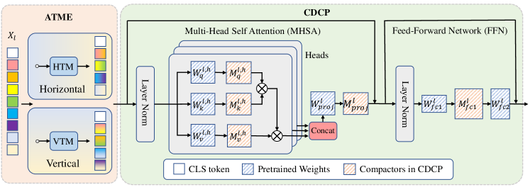
Figure 1: The overview of our proposed joint compression method for ViTs. We design an asymmetric token merging (ATME) strategy with horizontal token merging (HTM) and vertical token merging (VTM) to prune tokens while preserving their spatial integrity. Consistent dynamic channel pruning (CDCP) is further introduced to enable dynamic fine-grained compression optimization for all learnable weights with minimal performance degradation.

III-B Asymmetric Token Merging

Most existing token pruning methods focus solely on image classification, and generally reduce the number of tokens in an unstructured manner [27, 20, 28, 23, 30, 31, 32], i.e., by discarding tokens sparsely. However, although remarkable success has been achieved, sparsely wiping out redundant tokens inevitably disrupts the spatial integrity of images. Thus, the compressed ViT models are not suitable for downstream vision tasks that depend on a complete spatial structure, such as semantic segmentation, which significantly restricts their transferability. Here, we present an asymmetric token merging strategy to effectively accelerate ViTs, meanwhile maintaining the strong transferability of ViTs. Specifically, we introduce two basic token merging operations to integrate token features while preserving spatial integrity.

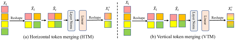
Figure 2: The proposed asymmetric token merging strategy prunes tokens horizontally or vertically.

Horizontal token merging (HTM). As shown in Figure 2.(a), for a sequence of tokens $X_{l}\in R^{N_{l}\times C}$ to be processed, we first reshape it to the shape of feature maps, i.e., $\overline{X}_{l}\in R^{H\times W\times C}$, where $H$ and $W$ are the height and width of features maps. Then, we group and concatenate two adjacent tokens horizontally, by which we can obtain $\widehat{X}_{l}\in R^{H\times\frac{W}{2}\times 2C}$, where $2C$ is the feature dimension after concatenation. We leverage a lightweight linear layer to effectively fuse the features of grouped tokens by $\widetilde{X}_{l}=\textsf{Linear}(\textsf{LayerNorm}(\widehat{X}_{l}))\in R^{H\times\frac{W}{2}\times C}$. We then reshape it back to obtain a sequence of tokens, i.e., $X^{*}_{l}\in R^{\frac{N_{l}}{2}\times C}$.

Vertical token merging (VTM). As shown in Figure 2.(b), similar to horizontal token merging, after obtaining $\overline{X}_{l}\in R^{H\times W\times C}$, we group and concatenate two adjacent tokens along the vertical direction, ending up with $\widehat{X}_{l}\in R^{\frac{H}{2}\times W\times 2C}$. Similarly, we can obtain the fused token features by $\widetilde{X}_{l}=\textsf{Linear}(\textsf{LayerNorm}(\widehat{X}_{l}))\in R^{\frac{H}{2}\times W\times C}$. Then, we can derive the final token features $X^{*}_{l}\in R^{\frac{N_{l}}{2}\times C}$ after decreasing the number of tokens by reshaping.

By leveraging these two basic operations, we can obtain asymmetric feature maps through asymmetric merging in ViTs. Besides, both operations are generic and plug-and-play. We can seamlessly integrate them into ViTs without complicated hyper-parameter tuning. Following [27, 28, 32, 20], we hierarchically alternatively utilize horizontal and vertical token merging before MHSA through the whole network for the token pruning. Specifically, we first prioritize the strategy of uniformly dividing layers for pruning based on the expected FLOPs reduction. For example, if the target FLOPs reduction ratio for token pruning for DeiT-Small is 43.3%, we initially select the 3-th layer and 7-th layer to perform HTM and VTM, respectively, resulting in a FLOPs reduction of 41.1%. Either HTM first or VTM first makes a negligible difference according to our results. Subsequently, minor adjustments are made to the positions of the pruning layers, to align better with the desired ratio of FLOPs reduction. For example, we then adjust the pruning layer from the 7-th to the 6-th layer, resulting in an exact FLOPs reduction of 43.3%. In this way, we can progressively reduce the number of tokens in ViTs while still maintaining the integrity of spatial structure.

III-C Consistent Dynamic Channel Pruning

Dynamic channel pruning. Two-stage channel pruning methods involve pruning a pretrained model and subsequently fine-tuning the pruned model [55, 56]. However, these methods have limitations due to the pruning process, in which irreversible pruning can lead to the unintended removal of crucial channels and cause irreparable loss. In contrast, dynamic channel pruning dynamically determines the importance of channels during fine-tuning and encourages unimportant channels to gradually approach zero importance [57, 58, 59]. After fine-tuning, channels converging to zero importance are eliminated, resulting in the compressed model. In such a way, important channels can be recovered during training, thus leading to improved overall performance. Previous works for dynamic channel pruning focus on the design of metrics for deciding the importance of channels. Among them, compactor-based method [57] achieves the state-of-the-art performance for CNN pruning. Here, we propose a consistent dynamic channel pruning strategy based on [57] to perform fine-grained compression optimization for all modules in ViTs.

As shown in Figure 3, following [57], we insert a compactor, which is a learnable transformation matrix, for each parameter in ViT. For the generality of description, we denote a compactor and its preceding weight as $M$ and $W$, respectively, if not specified. Otherwise, we add super/sub-scripts to them to indicate their positions. For example, $M^{l,h}_{q}\in R^{D\times D}$ denotes the compactor corresponding to $W^{l,h}_{q}$ for the $h$-th head in the $l$-th block. Intuitively, in the compactor $M$, each column $\boldsymbol{c}\in M$ is corresponding to one output channel of $W$. The norm of $\boldsymbol{c}$ can revel the importance of channels for $W$. Therefore, during training, we adopt the group lasso loss [60, 61] to dynamically push channels of $M$ to be sparse, i.e., $L_{lasso}=||\boldsymbol{c}||_{2}$. As [57], we introduce a mask variable $m\in\{0,1\}$ for each $\boldsymbol{c}$ to indicate the corresponding channel is pruned, i.e., $m=0$, or not, i.e., $m=1$. We update the gradient of $\boldsymbol{c}$ manually by

$$\bigtriangledown{c}=m\frac{\partial L_{cls}}{\partial\boldsymbol{c}}+\lambda\frac{\partial L_{lasso}}{\partial\boldsymbol{c}},$$ (2)

where $L_{cls}$ is the classification objective and $\lambda$ is a hyper-parameter. For every several iterations, we set the masks of $\boldsymbol{c}$ with the lowest norm values to 0 for encouraging the unimportant channels to approach zero importance. After training, we can eliminate redundant (converging to zero importance) channels in $M$, ending up with a pruned compactor $\overline{M}$. Then, a pruned weight, denoted as $\overline{W}$, can be derived by ${\overline{W}}=W{\overline{M}}$.

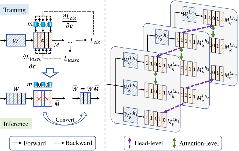
Figure 3: Left: Framework of the compactor. Right: Consistencies for pruning MHSA.

However, Vanilla compactor pruning techniques apply global selection criteria to identify unimportant channels and encourage them to approach zero importance. It may result in (1) imbalance sparse ratios of channels among heads after fine-tuning. Therefore, only the minimum ratio of near-zero importance channels across heads can be removed for efficient parallel self-attention computation; and (2) inconsistent channel importance between $W_{q}^{l,h}$ and $W_{k}^{l,h}$ which leads to different sparse outcomes. For example, one channel’s importance may be close to zero importance in the query while its corresponding one in the key it not. Therefore, only the channels with zero importance in both the query and key can be pruned for error-free self-attention computation. However, in such a way, a substantial number of near-zero importance channels are retained in the compressed model (see Figure 5), which degrades the performance (see Table VI). Here, to address such issues, we introduce head-level consistency and attention-level consistency for pruning ViTs, as shown in Figure 3. Specifically, we first formulate the importance score of channel $\boldsymbol{c}$ as $s=||\boldsymbol{c}||_{2}$. For channels with the same position in $M^{l,h}_{q}$ and $M^{l,h}_{k}$, their scores will be normalized as the mean of the corresponding original scores. Then, we can obtain a global set $S$, which contains scores of all channels in compactors. Meanwhile, we can derive local score sets, i.e., $S_{q}^{l,h}$, $S_{k}^{l,h}$ and $S_{v}^{l,h}$, for compactors in MHSA, i.e., $M_{q}^{l,h}$, $M_{k}^{l,h}$ and $M_{v}^{l,h}$, respectively. We initialize an empty set $P$ to record unimportant channels for removal. Then, we iteratively find unimportant channels and add them to $P$ until a pre-defined FLOPs reduction ratio $r_{target}$ is achieved.

Head-level consistency. We apply it to make sure that ratios of pruned channels across heads are the same. We take $M_{q}^{l,h}$ as an example. As shown in Algorithm 1, suppose we have selected a channel $\boldsymbol{c}\in M_{q}^{l,h}$ for pruning. For other head $h^{\prime}\neq h$, we remove the smallest score from the local score set $S_{q}^{l,h^{\prime}}$ (Algorithm 1) and add its corresponding channel $\boldsymbol{c}^{\prime}\in M_{q}^{l,h^{\prime}}$ to $P$ (Algorithm 1). In this way, after pruning, different heads in the same compactor will be in the same shape.

Input: Selected channel $\boldsymbol{c}\in M_{q}^{l,h}$, score sets for each head $\{S_{q}^{l,1},...,S_{q}^{l,h},...\}$

Output: Expanded to-be-pruned channels P

1 $S_{q}^{l,h}\leftarrow S_{q}^{l,h}\setminus\{s_{\boldsymbol{c}}\}$; $P\leftarrow\{\boldsymbol{c}\}$;

2 for each head $h^{\prime}\neq h$  do

3       $\boldsymbol{c}^{\prime}\leftarrow\mathop{\arg\min}_{\boldsymbol{c}^{\prime}\in M_{q}^{l,h^{\prime}}}(S_{q}^{l,h^{\prime}})$;

4       $P\leftarrow P\cup\{\boldsymbol{c}^{\prime}\}$; $S_{q}^{l,h^{\prime}}\leftarrow S_{q}^{l,h^{\prime}}\setminus\{s_{\boldsymbol{c}^{\prime}}\}$;

Algorithm 1 Head-level consistency

Attention-level consistency. It is designed to encourage the consistent behavior for channels in the same position between $M_{q}^{l,h}$ and $M_{k}^{l,h}$, besides the same normalized score for them. As shown in Algorithm 2, if the $i$-th channel in $M_{q}^{l,h}$, i.e., $\boldsymbol{c}$, is pruned, the $i$-th channel in $M_{k}^{l,h}$, i.e., $\boldsymbol{c}^{\prime}$, is removed as well. Channels in $M_{k}^{l,h}$ will be managed in the same way. As a result, the remained channels in query and key are well aligned, ensuring error-free interaction during attention.

Input: Selected channel $\boldsymbol{c}\in M_{q}^{l,h}$ , score sets $\{S_{q}^{l,h},S_{k}^{l,h}\}$

Output: Expanded to-be-pruned channels P

1 $S_{q}^{l,h}\leftarrow S_{q}^{l,h}\setminus\{s_{\boldsymbol{c}}\}$; $P\leftarrow\{\boldsymbol{c}\}$;

2 $i=index(M_{q}^{l,h},\boldsymbol{c})$; $\boldsymbol{c}^{\prime}\leftarrow M_{k}^{l,h}[i]$;

$P\leftarrow P\cup\{\boldsymbol{c}^{\prime}\}$; $S_{k}^{l,h}\leftarrow S_{k}^{l,h}\setminus\{s_{\boldsymbol{c}^{\prime}}\}$;

Algorithm 2 Attention-level consistency

Algorithm 3 illustrates the proposed consistent dynamic channel pruning process. During training, unconstrained channels, i.e., $\boldsymbol{c}\in M_{proj}^{l}\cup M_{fc1}^{l}$, are directly added to $P$. For channel $\boldsymbol{c}\in M_{q}^{l,h}\cup M_{k}^{l,h}$, we apply the proposed head-level consistency to it. After that, we employ the attention-level consistency to the newly to-be-pruned channels. For $\boldsymbol{c}\in M_{v}^{l,h}$, we only apply head-level consistency.

Input: Global importance score set $S$, target FLOPs reduction ratio $r_{target}$

Output: Channels to be pruned P, current FLOPs reduction ratio $r_{current}$

1 while $r_{current}<r_{target}$ do

2       $\boldsymbol{c}\leftarrow\mathop{\arg\min}_{c}{S}$;

3       if $\boldsymbol{c}\in M_{proj}^{l}\cup M_{fc1}^{l}$ then

4             $P\leftarrow P\cup\{\boldsymbol{c}\}$; $S\leftarrow S\setminus\{s_{\boldsymbol{c}}\}$;

5       else if $\boldsymbol{c}\in M_{v}^{l,h}$ then

6             $P_{head}\leftarrow$ Head-level consistency($\boldsymbol{c}$);

7             $P\leftarrow P\cup P_{head}$; $S\leftarrow S\setminus S_{P_{head}}$;

8       else if $\boldsymbol{c}\in M_{q}^{l,h}\cup M_{k}^{l,h}$ then

9             $P_{head}\leftarrow$ Head-level consistency($\boldsymbol{c}$);

10             for each channel $\boldsymbol{c}^{\prime}\in P_{head}$ do

11                   $P_{attn}\leftarrow$ Attention-level consistency($\boldsymbol{c}^{\prime}$);

12                   $P\leftarrow P\cup P_{attn}$; $S\leftarrow S\setminus S_{P_{attn}};$

13       Update $r_{current}$

Algorithm 3 Channel pruning with consistencies

IV Experiments

We first compare our method with state-of-the-arts on ImageNet [62] to verify the high performance and fast inference speed obtained by our method (Section IV-A), following [23, 24, 25]. Then, we investigate impacts of each component by comprehensive analyses on ImageNet, following [23] (Section IV-B). We also provide results of semantic segmentation on the ADE20k dataset [63] to verify the transferability of our method (Section IV-C). The float operations (FLOPs) of models are measured by fvcore and the throughput is evaluated on a single NVIDIA RTX-3090 GPU with a batch size of 256, by default. For compared methods, we utilize their published pretrained models to obtain throughputs.

TABLE I: Hyper-parameters during fine-tuning

hyper-parameter	value
optimizer	AdamW
base learning rate	1e-4
weight decay	0.05
optimizer momentum	$\beta_{1}$ = 0.99 (compactor), 0.9 (other) $\beta_{2}$ = 0.999
batch size	256 (Tiny/Small), 128 (Base)
learning rate schedule	cosine decay
warmup epochs	5
label smoothing	0.1
mixup	0.8
cutmix	1.0
drop path	0.1
exp. moving average (EMA)	0.99996
distillation loss	cross entropy loss
distillation-alpha	0.1 (Tiny), 0.25 (Small/Base)

TABLE II: Comparison with state-of-the-art methods on ImageNet.

Model	Param. (M)	FLOPs (G)	FLOPs ($\downarrow$%)	Throughput (im/s)	Speed ($\uparrow$)	Top-1 (%)
DeiT-Tiny	5.7	1.3	-	3384	1.0$\times$	72.2
S2ViTE [19]	4.2	1.0	23.7	-	-	70.1
SPViT [64]	4.9	1.0	23.1	3542	1.1$\times$	70.7
ToMe [31]	5.7	0.7	41.3	4952	1.5$\times$	71.3
UVC [25]	-	0.6	50.8	-	-	71.3
SAViT [24]	4.2	0.9	25.2	-	-	70.7
VTC-LFC [23]	5.1	0.7	46.7	3141	0.9$\times$	71.6
CAIT (ours)	5.1	0.6	50.5	5865	1.7$\times$	72.3
DeiT-Small	22.1	4.6	-	1574	1.0$\times$	79.8
EViT [28]	22.1	2.3	50.0	2856	1.8$\times$	78.5
IA-RED2 [30]	22.1	3.2	31.5	2301	1.5$\times$	79.1
dTPS [32]	22.8	3.0	34.8	2339	1.5$\times$	80.1
S2ViTE [19]	14.6	3.2	31.6	-	-	79.2
SPViT [64]	16.4	3.3	28.3	1601	1.0$\times$	78.3
ToMe [31]	22.1	2.7	41.3	2405	1.5$\times$	79.4
UVC [25]	-	2.3	49.6	-	-	78.8
SAViT [24]	14.7	3.1	33.5	-	-	80.1
VTC-LFC [23]	17.7	2.1	54.4	1711	1.1$\times$	79.8
CAIT (ours)	18.4	2.1	54.4	2968	1.9$\times$	80.2
DeiT-Base	86.4	17.6	-	580	1.0$\times$	81.8
EViT [28]	86.4	11.6	34.1	860	1.5$\times$	81.3
IA-RED2 [30]	86.4	11.8	33.0	797	1.4$\times$	80.3
S2ViTE [19]	56.8	11.8	33.1	-	-	82.2
SPViT [64]	62.3	11.7	33.1	600	1.0$\times$	81.6
UVC [25]	-	8.0	54.4	-	-	80.6
VTC-LFC [23]	63.5	7.5	57.6	707	1.2$\times$	81.3
CAIT (ours)	71.3	7.4	58.0	1206	2.1$\times$	81.6

IV-A Comparison with State-of-the-Arts on ImageNet

IV-A1 Implementation details

We evaluate our proposed method on three different sizes of DeiT [6], i.e., DeiT-Tiny, DeiT-Small, and DeiT-Base. Our experiments are deployed with Pytorch [65] on RTX-3090 GPUs. In CDCP, following [57], $r_{target}$ is initialized to zero, which is then increased by 0.025% every 25 iterations until achieving the given reduction ratio. Meanwhile, we re-construct $P$ every same iterations. Besides, we start to increase $r_{target}$ and re-construct $P$ after 30 epochs. $\lambda$ in Equation 2 is empirically set to 1e-5. Table I reports the detailed hyper-parameters during training, most of which are the same as [23].

IV-A2 Results

As shown in Table II, our proposed method can consistently outperform previous methods across all three models, as evidenced by superior performance in terms of the Top-1 accuracy, the FLOPs reduction ratio, and the inference speed. Specifically, under similar FLOPs reduction ratios, our method outperforms the state-of-the-art VTC-LFC [23] by 0.7% and 0.4% in terms of Top-1 accuracy on DeiT-Tiny and DeiT-Small, respectively. Compared with methods that obtain comparable accuracy to ours, such as dTPS [32] and SPViT [64], our method can achieve much higher FLOPs reductions. We can see that in the proposed method, the fruitful FLOPs reduction can be sufficiently transformed into the significant inference acceleration. Notably, our compressed DeiT-Tiny, DeiT-Small and DeiT-Base models can achieve 1.7$\times$, 1.9$\times$, and 2.1$\times$ inference speedups, respectively, while enjoying no or little accuracy drops. These results well demonstrate the effectiveness and the superiority of our method.

TABLE III: Ablation study on DeiT-Tiny and DeiT-Small.

Method	DeiT-Tiny			DeiT-Small
	Top-1	Param.	FLOPs $\downarrow$	Top-1	Param.	FLOPs $\downarrow$
Original	72.2	5.7M	-	79.8	22.1M	-
ATME	71.9	5.9M	50.2%	79.8	22.9M	54.4%
CDCP	71.9	4.2M	31.2%	79.8	13.9M	38.1%
CAIT	72.3	5.1M	50.5%	80.2	18.4M	54.4%

IV-B Model analyses

IV-B1 Ablation study

We conduct experiments with DeiT-Tiny and DeiT-Small, following [32, 23]. As shown in Table III, compared with original models, our ATME can obtain comparable accuracy while reducing 50.2% and 54.4% FLOPs for DeiT-Tiny and DeiT-Small, respectively. The proposed CDCP can obtain sufficient FLOPS reduction as well. These results can demonstrate the effectiveness of ATME and CDCP. We can also observe that, compared with CDCP, our ATME, as a token pruning method, can obtain superior performance. This result is consistent with observations in prior works [23, 22, 28] that for ViT models, compressing tokens can achieve more outcomes than compressing channels. Therefore, in practice, we follow  [23] to assign more FLOPs reduction ratio on ATME. Specifically, given a desired ratio of overall FLOPs reduction, we first prioritize the strategy of uniformly dividing layers for token pruning, and then adjust the FLOPs reduction ratio of channel pruning to exactly match the target overall FLOPs reduction. Compared with ATME and CDCP, the final model, CAIT, boosts the performance by 0.4% for both DeiT-Tiny and DeiT-Small, in terms of Top-1 accuracy. Compared with original models, CAIT can enjoy considerable performance gains with over 50% FLOPs reduction, well demonstrating the effectiveness and superiority of the proposed method.

IV-B2 Superiority to alternative methods

To verify the superiority of our proposed ATME and CDCP over existing token pruning and channel pruning methods, we conduct experiments on ImageNet with only compressing tokens, channels, and both. Following [23], we introduce two state-of-the-art token pruning methods, i.e., EViT [28] and LFE [23], and two state-of-the-art channel pruning methods, i.e., NViT [22] and LFS [23], on DeiT-Small, as baselines for ATME and CDCP, respectively. When compressing both tokens and channels, we select better token pruning baseline method, i.e., LFE [23] and better channel pruning baseline method, i.e., LFS [23] for combinations. Results of compared baselines are borrowed from [23] directly. For fair comparison, we employ our method with the same training setting as [23]. As shown in Table IV, our ATME outperforms EViT by 0.4% Top-1 accuracy under the same FLOPs reduction. Compared with LFE, our ATME achieves significantly faster inference speed while obtaining comparable accuracy. For channel pruning, our CDCP can outperform NViT and LFS by 0.9% and 0.4% accuracy gains, respectively. When compressing both tokens and channels, our joint compression method is still superior to other combinations, i.e., ATME+LFS, LFE+CDCP, and LFE+LFS. These experimental results well show the superiority of our ATME and CDCP over other methods.

TABLE IV: Results on DeiT-Small (Top-1: 79.8%).

Token Pruning	Channel Pruning	Top-1	FLOPs $\downarrow$	Speed
EViT	-	79.6	43.3%	1.7$\times$
LFE	-	80.1	43.3%	1.5$\times$
ATME	-	80.0	43.3%	1.8$\times$
-	NViT	78.9	32.8%	1.2$\times$
-	LFS	79.4	32.8%	1.2$\times$
-	CDCP	79.8	32.8%	1.2$\times$
LFE	LFS	79.1	55.0%	1.6$\times$
LFE	CDCP	79.6	55.0%	1.6$\times$
ATME	LFS	79.1	55.0%	2.0$\times$
ATME	CDCP	79.5	55.0%	2.0$\times$

IV-B3 Asymmetry in ATME

Here, we investigate the beneficial impacts of asymmetry in our ATME. We introduce three baseline methods: (1) simultaneously using horizontal and vertical token merging as one operation, denoted as “symmetry”, in which we group and concatenate four adjacent tokens in both horizontal and vertical directions, i.e., in a 2$\times$2 patch; (2) only using horizontal token merging; (3) only using vertical token merging. As shown in Table V, our ATME can obtain better performance. Specifically, compared with “symmetry”, ATME progressively reduces the number of tokens in a moderate way, forbidding drastic losses of token information, thus achieving a 0.7% accuracy gain. Compared with HTM and VTM, ATME can maintain a more regular spatial structure for patches, resulting in a 0.4% performance improvement. These results well demonstrate the effectiveness of asymmetry in our ATME.

IV-B4 Consistencies in CDCP

We verify the positive effects of head-level consistency and attention-level consistency used in CDCP. Additionally, we introduce S²ViTE [19] as the baseline method, because it is a remarkable state-of-the-art dynamic channel pruning method. As shown in Table VI, head-level and attention-level consistencies can consistently achieve performance improvements. Specifically, head-level consistency leads to a 1.4% (CDCP 72.7% vs “w/o head” 71.3%) accuracy gain. Attention-level consistency obtains a 0.6% (CDCP 72.7% vs “w/o attn” 72.1%) performance improvement. Besides, our CDCP significantly outperforms the baseline “w/o both” and S²ViTE [19]. These experimental results well demonstrate the superiority of fine-grained compression with head-level and attention-level consistencies for ViTs.

TABLE V: Asymmetry (DeiT-Tiny: 72.2%).

Method	Top-1		FLOPs $\downarrow$	Speed
symmetry	71.2		50.7%	1.9$\times$
HTM	71.5		49.6%	1.8$\times$
VTM	71.5		49.6%	1.8$\times$
ATME	71.9		50.2%	1.9$\times$

TABLE VI: Consistencies (DeiT-Tiny: 72.2%).

Method	Top-1		FLOPs $\downarrow$	Speed
S2ViTE [19]	70.1		23.7%	1.1$\times$
w/o both	71.0		25.1%	1.2$\times$
w/o head	71.3		25.1%	1.2$\times$
w/o attn	72.1		25.1%	1.2$\times$
CDCP	72.7		25.1%	1.2$\times$

IV-B5 Compression on other ViT models

To explore the performance of our method on other variants of ViTs, we conduct experiments on LV-ViT [66] and Swin Transformer [2], following [23]. Following [23], we adopt ATME and CDCP on LV-ViT, and employ CDCP to Swin. Meanwhile, to simplify, the proposed token labels in the original LV-ViT are not used during training. As shown in Table VII, our method can consistently achieve the state-of-the-art performance on both models. Specifically, on LV-ViT, our method outperforms VTC-LFC [23] with 0.4% higher accuracy while achieving significantly faster acceleration (CAIT 1.9$\times$ vs VTC-LFC 1.2$\times$). For Swin Transformer, our compressed model can also obtain accuracy gains of 0.5% and 0.3% compared with SPViT [64]/VTC-LFC [23], respectively, under the similar FLOPs reduction ratio. These results well demonstrate the generalization of our method on other ViT variants. Besides, we can observe that LV-ViT and Swin Transformer generally suffer more accuracy drop after pruning than DeiT, which is consistent with previous works [23]. We hypothesize the reason lies in the architectural differences among LV-ViT, Swin Transformer, and DeiT. Specifically, LV-ViT adopts a narrower expansion ratio in FFN and a deeper layout to improve efficiency. It also leverages token labeling to introduce individual location-specific supervision. Swin Transformer adopts the hierarchical structure and shifted window design to enhance efficiency. Therefore, LV-ViT and Swin Transformer exhibit less data-level (i.e., tokens) redundancy and model-level (i.e., parameters) redundancy, compared with DeiT. They thus suffer more accuracy drop after pruning than DeiT. Additionally, our proposed method can consistently outperform existing methods on LV-ViT and Swin Transformer. It well demonstrates the superiority of our method for pruning various ViTs.

TABLE VII: Results on LV-ViT and Swin Transformer.

Method	Top-1	FLOPs $\downarrow$	Speed	Method	Top-1	FLOPs $\downarrow$	Speed
LV-ViT-S [66]	83.2	-	1.0$\times$	Swin-Tiny [2]	81.1	-	1.0$\times$
NViT [22]+EViT [28]	81.5	49.2%	1.8$\times$	SPViT [64]	80.1	24.4%	-
VTC-LFC [23]	81.8	50.8%	1.2$\times$	VTC-LFC [23]	80.3	26.7%	1.2$\times$
CAIT	82.2	53.8%	1.9$\times$	CDCP	80.6	26.7%	1.2$\times$

TABLE VIII: Results on semantic segmentation.

	Semantic FPN [67]			UperNet [68]			Mask2Former [69]
Backbone	mIoU	En. sp.	Over. sp.	mIoU	En. sp.	Over. sp.	mIoU	En. sp.	Over. sp.
DeiT-Small	44.3	1.00$\times$	1.00$\times$	44.9	1.00$\times$	1.00$\times$	47.2	1.00$\times$	1.00$\times$
VTC-LFC-unstructured [23]	0.1	1.01$\times$	1.01$\times$	0.1	1.01$\times$	1.01$\times$	45.2	1.16$\times$	1.05$\times$
VTC-LFC-structured [23]	43.5	1.01$\times$	1.00$\times$	44.2	1.00$\times$	1.00$\times$	46.3	1.15$\times$	1.05$\times$
Evo-ViT [33]	42.7	1.34$\times$	1.20$\times$	43.0	1.33$\times$	1.18$\times$	45.9	1.41$\times$	1.14$\times$
ATME	44.5	1.46$\times$	1.27$\times$	45.3	1.43$\times$	1.23$\times$	47.6	1.54$\times$	1.18$\times$
CAIT	44.5	1.52$\times$	1.31$\times$	45.6	1.48$\times$	1.26$\times$	47.2	1.64$\times$	1.21$\times$

IV-C Results on Semantic Segmentation

Most existing token pruning methods generally reduce the number of tokens in an unstructured manner [27, 20, 28, 23, 30, 31, 32], i.e., by dropping tokens sparsely, which however inevitably disrupts the complete spatial structure of images. Therefore, the accelerated ViTs are not suitable for downstream pixel-level vision tasks, like semantic segmentation. To verify the impact of unstructured token pruning on downstream vision tasks, we conduct experiments with the start-of-the-art VTC-LFC [23] on the ADE20k [63] dataset. Additionally, in contrast, our proposed method can preserve the spatial integrity and effectively adapt to downstream tasks that need a complete spatial structure of images. Therefore, we also conduct experiments on the ADE20k dataset to verify such a transferability. We introduce the state-of-the-art Evo-ViT [33] as one baseline method, which can also maintain the spatial structure of input images as ours.

IV-C1 Implementation details

Following [39, 66], we integrate the accelerated backbones into three advanced segmentation methods, i.e., Semantic FPN [67], UperNet [68], and Mask2Former [69]. We train for 80k, 160k and 160k iterations for these three segmentation methods, respectively. Besides, we adopt the AdamW optimizer with the learning rate of 6e-5 and weight decay of 0.01, as in [2]. The input resolution is set to 512$\times$512 and all models are trained using batch size of 32. We report the performance with standard single scale protocol as in  [39, 66]. Additionally, the encoder speedup (En. sp.) and overall speedup (Over. sp) are evaluated on a single RTX-3090 GPU with a batch size of 32, where the encoder contains the backbone, upsampling and downsampling modules. Our implementation is based on the mmsegmentation library [70].

IV-C2 Results

As VTC-LFC [23] produces sparse feature maps, following [71, 72], we use mask tokens to fill the dropped positions before feeding them into the semantic segmentation decoder, which is denoted as “VTC-LFC-unstructured”. As shown in Table VIII, due to the impaired spatial integrity of feature maps, CNN-based decoders, i.e., Semantic FPN[67] and UperNet [68], result in poor results. It is consistent with observations in previous works [72, 73] that CNNs exhibit significantly worse performance when dealing with sparse feature maps, which can be attributed to the disrupted data distribution of pixel values and vanished patterns of visual representations. Besides, with the Transformer-based decoder, i.e., Mask2Former [69], “VTC-LFC-unstructured” demonstrates a significant inferiority to DeiT-Small, with a considerable margin of 2.0% mIoU. These results well show the harmful impacts caused by unstructured token pruning when transferring the accelerated model to downstream structured vision task of semantic segmentation. Furthermore, we propose to record the dropped tokens and then use them to fill the corresponding positions when constructing feature maps for fed into the segmentation decoder, thus ensuring the spatial integrity of patches, which is denoted as “VTC-LFC-structured”. As shown in Table VIII, reasonably, “VTC-LFC-structured” outperforms “VTC-LFC-unstructured” across three segmentation methods.

Furthermore, as shown in Table VIII, our method not only exhibits superior performance but also boasts fast inference speed across all semantic segmentation methods. Specifically, our ATME yields impressive overall speedups of 1.27$\times$, 1.23$\times$, and 1.18$\times$, respectively, across three distinct segmentation methods, while maintaining optimal performance. Our ATME outperforms “VTC-LFC-structured” by great margins of 1%, 1.1%, 1.3% mIoUs on all segmentation decoders, respectively, with notably faster inference speedup. Besides, our ATME significantly outperforms Evo-ViT [33] with 1.8%, 2.3%, and 1.7% mIoU on three segmentation heads, respectively. It well indicates the superiority of asymmetric token merging in preserving spatial integrity, compared with Evo-ViT that can potentially harm token features. Besides, on top of ATME, our CAIT can further enhance the overall inference speed. These results well demonstrate the remarkable adaptability of the proposed method to downstream vision tasks.

TABLE IX: Impact of different usages of ATME.

Method	Top-1 (%)	Param. (M)	FLOPs (G)	Speed
DeiT-Tiny	72.2	5.7	1.3	1.0$\times$
DeiT-half depth	64.0	3.0	0.6	1.9$\times$
DeiT-half dim	66.3	2.8	0.6	1.2$\times$
ATME-scratch	71.1	5.9	0.6	1.9$\times$
ATME	71.9	5.9	0.6	1.9$\times$

IV-D Discussion

IV-D1 Insightful analyses for ATME

Here, we provide more insightful analyses for ATME. The proposed ATME uniformly aggregates features of neighboring tokens, which can be regarded as a general architecture for modern ViTs. Therefore, we construct a vision transformer model whose architecture is the same as our ATME. Then, we train this model for 600 epochs from scratch with hard distillation of the pretrained model, following the scheme of training DeiT-Tiny [6]. We denote this model as “ATME-scratch”. Besides, we introduce two additional models whose FLOPs are similar to ATME-scratch’s. One involves halving the depth of DeiT-Tiny, which reduces the number of blocks. The other involves halving the width of DeiT-Tiny, which reduces the embedding dimension. We denote these two models as “DeiT-half depth” and “DeiT-half dim”, respectively, which are trained under the same setting as “ATME-scratch”. We compare these three models with the one obtained by our ATME pruning method. As shown in Table IX, “ATME-scratch” significantly outperforms “DeiT-half depth” and “DeiT-half dim” by 7.1% and 4.8% in terms of Top-1 accuracy, respectively. This may be attributed to the inductive bias of locality introduced by our ATME strategy. Moreover, “ATME-scratch” is inferior to DeiT-Tiny by a great margin of 1.1% accuracy. In contrast, our ATME can result in only a 0.3% drop, compared with vanilla DeiT-Tiny, while achieving a superior speedup of 1.9$\times$. It indicates that in addition to introducing the locality, our ATME can further preserve the pretrained model’s ability to capture visual features and prevent knowledge forgetting during pruning. Thanks to them, our ATME can well serve as a compression methodology for ViTs, delivering high performance and fast inference speed.

TABLE X: Comparison with ToMe on ImageNet. * indicates that ToMe is adopted in the same pruning layers as ATME.

Method	Top-1 (%)	FLOPs $\downarrow$	Speed
DeiT-Small	79.8	-	1.0$\times$
ToMe	79.9	41.3%	1.7$\times$
ToMe*	80.0	41.6%	1.5$\times$
ATME	80.0	43.3%	1.8$\times$

TABLE XI: Comparison with ToMe on ADE20k using Semantic FPN. * indicates that ToMe is adopted in the same pruning layers as ATME.

Method	mIoU	FLOPs $\downarrow$	Overall speed
DeiT-Small	44.3	-	1.00$\times$
ToMe	44.0	41.3%	1.06$\times$
ToMe*	43.9	41.6%	1.22$\times$
ATME	44.5	43.3%	1.27$\times$

IV-D2 Comparison between ATME and ToMe

TOME is an existing state-of-the-art token pruning method, which leverage bipartite soft matching to merge similar tokens. To demonstrate the superiority of our proposed ATME for token pruning, we compare our strategy with two variants: (1) using the strategy in ToMe in the same pruning layers as our ATME; and (2) performing ToMe at every layer as in their paper [31].

We first conduct experiments on ImageNet under the same setting to investigate their performance based on DeiT-Small. As shown in Table X, our ATME obtains a comparable accuracy with ToMe and ToMe* under a larger FLOPs reduction, demonstrating the effectiveness of our asymmetric token merging method. Besides, the strategy in ToMe employs a complex bipartite similarity matching with complex operators, while our ATME simply merges neighboring tokens and utilize fast tensor manipulations. Our ATME thus affords a significant advantage for various devices and platforms, particularly those with limited computation ability or lacking support for complex operators. As evidenced in Table X, our ATME is more friendly to latency and leads to an advantageous inference speedup compared with ToMe and ToMe*. These results well demonstrates the effectiveness of our proposed ATME.

More importantly, the strategy in ToMe merges tokens sparsely at each pruning layer, resulting in the disruption of the spatial integrity of images and restricting the transferability of compressed models to downstream structured vision tasks. In contrast, our ATME can well preserve the complete structure of patches and maintain the strong transferability of ViTs. We further conduct experiments on the downstream semantic segmentation task to verify this, by Semantic FPN segmentation method. To transfer the strategy in ToMe to the downstream task, we track which tokens get merged and then unmerge tokens, i.e., using the merged token to fill the corresponding empty positions, when constructing feature maps for fed into the segmentation decoder. As shown in Table XI, our ATME outperforms ToMe and ToMe* with considerable margins of 0.5 and 0.6 mIoUs, along with a larger overall inference speedup. These results well demonstrates the superiority of our method in transferability.

TABLE XII: ATME in Hierarchical Architectures.

Method	Top-1 (%)	FLOPs $\downarrow$	Speed
Swin-Tiny [2]	81.1	-	1.0$\times$
CDCP	80.6	26.7%	1.2$\times$
CAIT	80.5	35.4%	1.3$\times$

IV-D3 ATME in Hierarchical Architectures

As an efficient token pruning strategy for DeiT, our proposed ATME can also transfer to hierarchical architectures, e.g., Swin Transformer. We conduct experiments under the same setting in Section IV-B5 to verify this. Specifically, we adopt HTM and VTM at the last two layers of the 3-th Stage in Swin-Tiny, respectively, which results in a FLOPs reduction of 20.1%. We further perform channel pruning on it, leading to an overall 35.4% FLOPs reduction. As shown in Table XII, CAIT obtains a comparable accuracy with only performing channel pruning on Swin-Tiny, but with a much larger FLOPs reduction (35.4% vs. 26.7%) and a more significant inference speedup (1.3x vs. 1.2x). It well demonstrates the effectiveness of our token compression method in transferring to hierarchical architectures.

TABLE XIII: Results for different warmup epochs on DeiT-Tiny.

warmup epochs	Top-1 (%)	FLOPs $\downarrow$	Speed
0	72.26	50.5%	1.7$\times$
15	72.31	50.5%	1.7$\times$
30	72.34	50.5%	1.7$\times$

TABLE XIV: Results for different interval iterations on DeiT-Tiny.

interval iterations	Top-1 (%)	FLOPs $\downarrow$	Speed
25	72.34	50.5%	1.7$\times$
50	72.37	50.5%	1.7$\times$
75	72.46	50.5%	1.7$\times$

IV-D4 Compression schedule of CDCP

We follow [57] to set the compression training schedule of CDCP. To verify that the pruning performance of our CDCP is not sensitive to different compression schedules, we conduct experiments on DeiT-Tiny to analyze the effects of the warmup epochs and interval iterations for the reconstruction of $P$. As shown in Table XIII and Table XIV, we can see that they do not make significant differences, indicating the robustness of CDCP. These results well demonstrate the effectiveness of our method is general and not limited by specific schedules.

TABLE XV: Results for different fine-tuning epochs on DeiT-Small. The suffix ”-Xe” means X epochs.

Method	Top-1 (%)	FLOPs ($\downarrow$)	Speed
DeiT-Small	79.8	-	1.0$\times$
CAIT-30e	76.7	55.0%	2.0$\times$
CAIT-150e	79.5	55.0%	2.0$\times$
CAIT-300e	80.2	55.0%	2.0$\times$

IV-D5 Different fine-tuning epochs for CAIT

To investigate the performance of different fine-tuning epochs of our CAIT, we conduct experiments on DeiT-Small. As shown in Table XV, due to introducing parameters for extra optimization, our method benefits more from longer fine-tuning epochs, and results in a high performance upper bound. Specifically, our CAIT-150e and CAIT-300e enjoys a 2.0$\times$ inference speedup with no or little accuracy drops. These results well demonstrate the superiority and effectiveness of our CAIT.

IV-D6 Parameter distribution of pruned models

Here, we visualize the parameter distribution of pruned DeiT-Tiny, DeiT-Small and DeiT-Base. Figure 4 presents the saved ratios of channels in each block. It reveals that middle and deep blocks tend to retain more channels than shallow blocks, which is consistent with observations in prior works [23, 24]. This phenomenon may be attributed to the fact that middle and deep blocks incorporate more global context and thus capture more complex visual representations. Furthermore, it may provide some insight towards the construction of efficient ViTs. For example, we can maintain narrower channels in the shallow blocks of ViTs.

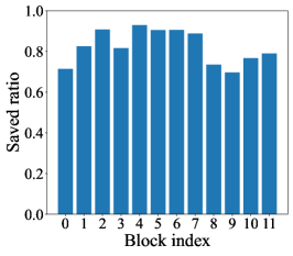
(a)

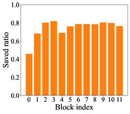
(b)

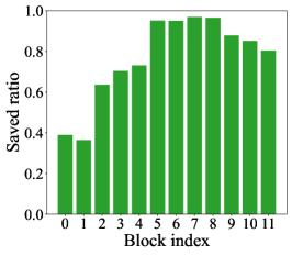
(c)

Figure 4: Architecture of pruned (a) DeiT-Tiny, (b) DeiT-Small, and (c) DeiT-Base models.

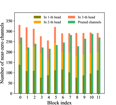
(a) w/o consistencies

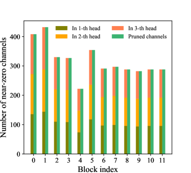
(b) w/ consistencies

Figure 5: Near-zero importance channels VS. Pruned channels in MHSA.

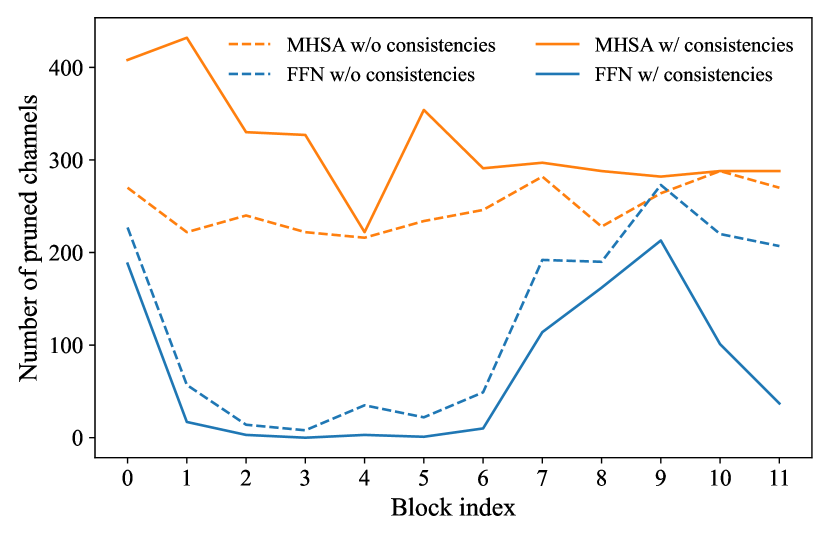
Figure 6: Pruned channels in MHSA and FFN modules

IV-D7 Visualization of consistencies

Here, we conduct visualization analyses to show the positive effects of our proposed head-level consistency and attention-level consistency in CDCP. Specifically, we visualize the near-zero importance channels in each head and the ultimately pruned channels in the MHSA module, based on the DeiT-Tiny model with three heads. As mentioned in Section III-C, directly applying the conventional compactor pruning strategy for ViTs will cause imbalance ratios of pruned channels among heads and inconsistent pruned channels between query and key transformation matrices, leading to difficulties for parallel and error-free self-attention computation. Then, only the minimum ratio of near-zero importance channels among heads can be pruned and only the consistent near-zero importance channels between query and key transformation matrices can be removed. However, as shown in Figure 5.(a), such a strategy will cause a substantial number of channels close to zero importance are retained in the compressed model, which impacts the performance adversely (see Table VI). In contrast, our head-level and attention-level consistencies can maintain different heads of the same block in the same shape, and well align remained channels in the query and key, respectively. Therefore, as shown in Figure 5.(b), our proposed consistencies can well address the limitations of vanilla compactor pruning on ViTs, ensuring error-free parallel self-attention computation and leading to superior performance (see Table 5 in the paper). Besides, as shown in Figure 6, we can also observe that our proposed consistencies result in more pruned channels in MHSA modules and less pruned channels in FFN modules. This may be attributed to the fact that we encourage consistent shapes of different heads and aligned channels of the query and key in MHSA during pruning. It is also consistent with observations in previous works [22, 74, 75] that more redundant channels lie in MHSA modules. Additionally, results in Table 5 in the paper demonstrate the effectiveness of such a pruning strategy.

V Conclusion

In this paper, we proposes a joint compression method with asymmetric token merging and consistent dynamic channel pruning for ViTs. The proposed asymmetric token merging strategy can effectively reduce the number of tokens while maintaining the spatial structure of images. The consistent dynamic channel pruning strategy can perform dynamic fine-grained compression optimization for all modules in ViTs. Extensive experiments on multiple ViTs over image classification and semantic segmentation show that our method can outperform state-of-the-art methods, achieving high performance, fast inference speed, and favorable transferability at the same time, well demonstrating its effectiveness and superiority.

References

- [1] A. Dosovitskiy, L. Beyer, A. Kolesnikov, D. Weissenborn, X. Zhai, T. Unterthiner, M. Dehghani, M. Minderer, G. Heigold, S. Gelly et al., “An image is worth 16x16 words: Transformers for image recognition at scale,” arXiv preprint arXiv:2010.11929, 2020.
- [2] Z. Liu, Y. Lin, Y. Cao, H. Hu, Y. Wei, Z. Zhang, S. Lin, and B. Guo, “Swin transformer: Hierarchical vision transformer using shifted windows,” in Proceedings of the IEEE/CVF international conference on computer vision, 2021, pp. 10 012–10 022.
- [3] X. Dong, J. Bao, D. Chen, W. Zhang, N. Yu, L. Yuan, D. Chen, and B. Guo, “Cswin transformer: A general vision transformer backbone with cross-shaped windows,” in Proceedings of the IEEE/CVF Conference on Computer Vision and Pattern Recognition, 2022, pp. 12 124–12 134.
- [4] Y. Li, C.-Y. Wu, H. Fan, K. Mangalam, B. Xiong, J. Malik, and C. Feichtenhofer, “Improved multiscale vision transformers for classification and detection,” arXiv preprint arXiv:2112.01526, 2021.
- [5] S. Wu, T. Wu, H. Tan, and G. Guo, “Pale transformer: A general vision transformer backbone with pale-shaped attention,” in Proceedings of the AAAI Conference on Artificial Intelligence, vol. 36, no. 3, 2022, pp. 2731–2739.
- [6] H. Touvron, M. Cord, M. Douze, F. Massa, A. Sablayrolles, and H. Jégou, “Training data-efficient image transformers & distillation through attention,” in International conference on machine learning. PMLR, 2021, pp. 10 347–10 357.
- [7] A. Amini, A. S. Periyasamy, and S. Behnke, “T6d-direct: Transformers for multi-object 6d pose direct regression,” in Pattern Recognition: 43rd DAGM German Conference, DAGM GCPR 2021, Bonn, Germany, September 28–October 1, 2021, Proceedings. Springer, 2022, pp. 530–544.
- [8] S. Zheng, J. Lu, H. Zhao, X. Zhu, Z. Luo, Y. Wang, Y. Fu, J. Feng, T. Xiang, P. H. Torr et al., “Rethinking semantic segmentation from a sequence-to-sequence perspective with transformers,” in Proceedings of the IEEE/CVF conference on computer vision and pattern recognition, 2021, pp. 6881–6890.
- [9] S. He, H. Luo, P. Wang, F. Wang, H. Li, and W. Jiang, “Transreid: Transformer-based object re-identification,” in Proceedings of the IEEE/CVF international conference on computer vision, 2021, pp. 15 013–15 022.
- [10] H. Chen, Y. Wang, T. Guo, C. Xu, Y. Deng, Z. Liu, S. Ma, C. Xu, C. Xu, and W. Gao, “Pre-trained image processing transformer,” in Proceedings of the IEEE/CVF Conference on Computer Vision and Pattern Recognition, 2021, pp. 12 299–12 310.
- [11] J. Wei, Y. Tay, R. Bommasani, C. Raffel, B. Zoph, S. Borgeaud, D. Yogatama, M. Bosma, D. Zhou, D. Metzler et al., “Emergent abilities of large language models,” arXiv preprint arXiv:2206.07682, 2022.
- [12] A. Chowdhery, S. Narang, J. Devlin, M. Bosma, G. Mishra, A. Roberts, P. Barham, H. W. Chung, C. Sutton, S. Gehrmann et al., “Palm: Scaling language modeling with pathways,” arXiv preprint arXiv:2204.02311, 2022.
- [13] O. OpenAI, “Gpt-4 technical report,” Mar 2023.
- [14] X. Chen, X. Wang, S. Changpinyo, A. Piergiovanni, P. Padlewski, D. Salz, S. Goodman, A. Grycner, B. Mustafa, L. Beyer et al., “Pali: A jointly-scaled multilingual language-image model,” arXiv preprint arXiv:2209.06794, 2022.
- [15] C. Riquelme, J. Puigcerver, B. Mustafa, M. Neumann, R. Jenatton, A. Susano Pinto, D. Keysers, and N. Houlsby, “Scaling vision with sparse mixture of experts,” Advances in Neural Information Processing Systems, vol. 34, pp. 8583–8595, 2021.
- [16] X. Zhai, A. Kolesnikov, N. Houlsby, and L. Beyer, “Scaling vision transformers,” in Proceedings of the IEEE/CVF Conference on Computer Vision and Pattern Recognition, 2022, pp. 12 104–12 113.
- [17] M. Dehghani, J. Djolonga, B. Mustafa, P. Padlewski, J. Heek, J. Gilmer, A. Steiner, M. Caron, R. Geirhos, I. Alabdulmohsin et al., “Scaling vision transformers to 22 billion parameters,” arXiv preprint arXiv:2302.05442, 2023.
- [18] A. Kirillov, E. Mintun, N. Ravi, H. Mao, C. Rolland, L. Gustafson, T. Xiao, S. Whitehead, A. C. Berg, W.-Y. Lo et al., “Segment anything,” arXiv preprint arXiv:2304.02643, 2023.
- [19] T. Chen, Y. Cheng, Z. Gan, L. Yuan, L. Zhang, and Z. Wang, “Chasing sparsity in vision transformers: An end-to-end exploration,” Advances in Neural Information Processing Systems, vol. 34, pp. 19 974–19 988, 2021.
- [20] Z. Kong, P. Dong, X. Ma, X. Meng, W. Niu, M. Sun, X. Shen, G. Yuan, B. Ren, H. Tang et al., “Spvit: Enabling faster vision transformers via latency-aware soft token pruning,” in Computer Vision–ECCV 2022: 17th European Conference, Tel Aviv, Israel, October 23–27, 2022, Proceedings, Part XI. Springer, 2022, pp. 620–640.
- [21] M. Zhu, Y. Tang, and K. Han, “Vision transformer pruning,” arXiv preprint arXiv:2104.08500, 2021.
- [22] H. Yang, H. Yin, P. Molchanov, H. Li, and J. Kautz, “Nvit: Vision transformer compression and parameter redistribution,” arXiv preprint arXiv:2110.04869, 2021.
- [23] Z. Wang, H. Luo, P. Wang, F. Ding, F. Wang, and H. Li, “Vtc-lfc: Vision transformer compression with low-frequency components,” Advances in Neural Information Processing Systems, vol. 35, pp. 13 974–13 988, 2022.
- [24] C. Zheng, K. Zhang, Z. Yang, W. Tan, J. Xiao, Y. Ren, S. Pu et al., “Savit: Structure-aware vision transformer pruning via collaborative optimization,” Advances in Neural Information Processing Systems, vol. 35, pp. 9010–9023, 2022.
- [25] S. Yu, T. Chen, J. Shen, H. Yuan, J. Tan, S. Yang, J. Liu, and Z. Wang, “Unified visual transformer compression,” arXiv preprint arXiv:2203.08243, 2022.
- [26] Y. Tang, K. Han, Y. Wang, C. Xu, J. Guo, C. Xu, and D. Tao, “Patch slimming for efficient vision transformers,” in Proceedings of the IEEE/CVF Conference on Computer Vision and Pattern Recognition, 2022, pp. 12 165–12 174.
- [27] Y. Rao, W. Zhao, B. Liu, J. Lu, J. Zhou, and C.-J. Hsieh, “Dynamicvit: Efficient vision transformers with dynamic token sparsification,” Advances in neural information processing systems, vol. 34, pp. 13 937–13 949, 2021.
- [28] Y. Liang, C. Ge, Z. Tong, Y. Song, J. Wang, and P. Xie, “Not all patches are what you need: Expediting vision transformers via token reorganizations,” arXiv preprint arXiv:2202.07800, 2022.
- [29] Z. Hou and S.-Y. Kung, “Multi-dimensional model compression of vision transformer,” in 2022 IEEE International Conference on Multimedia and Expo (ICME). IEEE, 2022, pp. 01–06.
- [30] B. Pan, R. Panda, Y. Jiang, Z. Wang, R. Feris, and A. Oliva, “Ia-red 2: Interpretability-aware redundancy reduction for vision transformers,” Advances in Neural Information Processing Systems, vol. 34, pp. 24 898–24 911, 2021.
- [31] D. Bolya, C.-Y. Fu, X. Dai, P. Zhang, C. Feichtenhofer, and J. Hoffman, “Token merging: Your vit but faster,” arXiv preprint arXiv:2210.09461, 2022.
- [32] S. Wei, T. Ye, S. Zhang, Y. Tang, and J. Liang, “Joint token pruning and squeezing towards more aggressive compression of vision transformers,” in Proceedings of the IEEE/CVF Conference on Computer Vision and Pattern Recognition, 2023, pp. 2092–2101.
- [33] Y. Xu, Z. Zhang, M. Zhang, K. Sheng, K. Li, W. Dong, L. Zhang, C. Xu, and X. Sun, “Evo-vit: Slow-fast token evolution for dynamic vision transformer,” in Proceedings of the AAAI Conference on Artificial Intelligence, vol. 36, no. 3, 2022, pp. 2964–2972.
- [34] A. Vaswani, N. Shazeer, N. Parmar, J. Uszkoreit, L. Jones, A. N. Gomez, Ł. Kaiser, and I. Polosukhin, “Attention is all you need,” Advances in neural information processing systems, vol. 30, 2017.
- [35] J. Guo, K. Han, H. Wu, Y. Tang, X. Chen, Y. Wang, and C. Xu, “Cmt: Convolutional neural networks meet vision transformers,” in Proceedings of the IEEE/CVF Conference on Computer Vision and Pattern Recognition, 2022, pp. 12 175–12 185.
- [36] H. Bao, L. Dong, S. Piao, and F. Wei, “Beit: Bert pre-training of image transformers,” arXiv preprint arXiv:2106.08254, 2021.
- [37] L. Yuan, Y. Chen, T. Wang, W. Yu, Y. Shi, Z.-H. Jiang, F. E. Tay, J. Feng, and S. Yan, “Tokens-to-token vit: Training vision transformers from scratch on imagenet,” in Proceedings of the IEEE/CVF international conference on computer vision, 2021, pp. 558–567.
- [38] C.-F. R. Chen, Q. Fan, and R. Panda, “Crossvit: Cross-attention multi-scale vision transformer for image classification,” in Proceedings of the IEEE/CVF international conference on computer vision, 2021, pp. 357–366.
- [39] A. Ali, H. Touvron, M. Caron, P. Bojanowski, M. Douze, A. Joulin, I. Laptev, N. Neverova, G. Synnaeve, J. Verbeek et al., “Xcit: Cross-covariance image transformers,” Advances in neural information processing systems, vol. 34, pp. 20 014–20 027, 2021.
- [40] B. Graham, A. El-Nouby, H. Touvron, P. Stock, A. Joulin, H. Jégou, and M. Douze, “Levit: a vision transformer in convnet’s clothing for faster inference,” in Proceedings of the IEEE/CVF international conference on computer vision, 2021, pp. 12 259–12 269.
- [41] P. Wang, X. Wang, F. Wang, M. Lin, S. Chang, H. Li, and R. Jin, “Kvt: k-nn attention for boosting vision transformers,” in Computer Vision–ECCV 2022: 17th European Conference, Tel Aviv, Israel, October 23–27, 2022, Proceedings, Part XXIV. Springer, 2022, pp. 285–302.
- [42] X. Chen, C.-J. Hsieh, and B. Gong, “When vision transformers outperform resnets without pre-training or strong data augmentations,” arXiv preprint arXiv:2106.01548, 2021.
- [43] X. Zhu, W. Su, L. Lu, B. Li, X. Wang, and J. Dai, “Deformable detr: Deformable transformers for end-to-end object detection,” arXiv preprint arXiv:2010.04159, 2020.
- [44] Z. Dai, B. Cai, Y. Lin, and J. Chen, “Up-detr: Unsupervised pre-training for object detection with transformers,” in Proceedings of the IEEE/CVF conference on computer vision and pattern recognition, 2021, pp. 1601–1610.
- [45] I. Misra, R. Girdhar, and A. Joulin, “An end-to-end transformer model for 3d object detection,” in Proceedings of the IEEE/CVF International Conference on Computer Vision, 2021, pp. 2906–2917.
- [46] A. El-Nouby, N. Neverova, I. Laptev, and H. Jégou, “Training vision transformers for image retrieval,” arXiv preprint arXiv:2102.05644, 2021.
- [47] B. Cheng, A. Schwing, and A. Kirillov, “Per-pixel classification is not all you need for semantic segmentation,” Advances in Neural Information Processing Systems, vol. 34, pp. 17 864–17 875, 2021.
- [48] Y. Wang, Z. Xu, X. Wang, C. Shen, B. Cheng, H. Shen, and H. Xia, “End-to-end video instance segmentation with transformers,” in Proceedings of the IEEE/CVF conference on computer vision and pattern recognition, 2021, pp. 8741–8750.
- [49] L. Ding, D. Lin, S. Lin, J. Zhang, X. Cui, Y. Wang, H. Tang, and L. Bruzzone, “Looking outside the window: Wide-context transformer for the semantic segmentation of high-resolution remote sensing images. arxiv 2021,” arXiv preprint arXiv:2106.15754.
- [50] F. Yang, H. Yang, J. Fu, H. Lu, and B. Guo, “Learning texture transformer network for image super-resolution,” in Proceedings of the IEEE/CVF conference on computer vision and pattern recognition, 2020, pp. 5791–5800.
- [51] X. Lai, J. Liu, L. Jiang, L. Wang, H. Zhao, S. Liu, X. Qi, and J. Jia, “Stratified transformer for 3d point cloud segmentation,” in Proceedings of the IEEE/CVF Conference on Computer Vision and Pattern Recognition, 2022, pp. 8500–8509.
- [52] M. S. Ryoo, A. Piergiovanni, A. Arnab, M. Dehghani, and A. Angelova, “Tokenlearner: What can 8 learned tokens do for images and videos?” arXiv preprint arXiv:2106.11297, 2021.
- [53] J. Zhang, H. Peng, K. Wu, M. Liu, B. Xiao, J. Fu, and L. Yuan, “Minivit: Compressing vision transformers with weight multiplexing,” in Proceedings of the IEEE/CVF Conference on Computer Vision and Pattern Recognition, 2022, pp. 12 145–12 154.
- [54] Z. Zong, K. Li, G. Song, Y. Wang, Y. Qiao, B. Leng, and Y. Liu, “Self-slimmed vision transformer,” in Computer Vision–ECCV 2022: 17th European Conference, Tel Aviv, Israel, October 23–27, 2022, Proceedings, Part XI. Springer, 2022, pp. 432–448.
- [55] Y. He, G. Kang, X. Dong, Y. Fu, and Y. Yang, “Soft filter pruning for accelerating deep convolutional neural networks,” arXiv preprint arXiv:1808.06866, 2018.
- [56] Y. He, P. Liu, Z. Wang, Z. Hu, and Y. Yang, “Filter pruning via geometric median for deep convolutional neural networks acceleration,” in Proceedings of the IEEE/CVF conference on computer vision and pattern recognition, 2019, pp. 4340–4349.
- [57] X. Ding, T. Hao, J. Tan, J. Liu, J. Han, Y. Guo, and G. Ding, “Resrep: Lossless cnn pruning via decoupling remembering and forgetting,” in Proceedings of the IEEE/CVF International Conference on Computer Vision, 2021, pp. 4510–4520.
- [58] S. Lin, R. Ji, Y. Li, Y. Wu, F. Huang, and B. Zhang, “Accelerating convolutional networks via global & dynamic filter pruning.” in IJCAI, vol. 2, no. 7. Stockholm, 2018, p. 8.
- [59] Z. Hou, M. Qin, F. Sun, X. Ma, K. Yuan, Y. Xu, Y.-K. Chen, R. Jin, Y. Xie, and S.-Y. Kung, “Chex: channel exploration for cnn model compression,” in Proceedings of the IEEE/CVF Conference on Computer Vision and Pattern Recognition, 2022, pp. 12 287–12 298.
- [60] B. Liu, M. Wang, H. Foroosh, M. Tappen, and M. Pensky, “Sparse convolutional neural networks,” in Proceedings of the IEEE conference on computer vision and pattern recognition, 2015, pp. 806–814.
- [61] W. Wen, C. Wu, Y. Wang, Y. Chen, and H. Li, “Learning structured sparsity in deep neural networks,” Advances in neural information processing systems, vol. 29, 2016.
- [62] O. Russakovsky, J. Deng, H. Su, J. Krause, S. Satheesh, S. Ma, Z. Huang, A. Karpathy, A. Khosla, M. Bernstein et al., “Imagenet large scale visual recognition challenge,” International journal of computer vision, vol. 115, pp. 211–252, 2015.
- [63] B. Zhou, H. Zhao, X. Puig, S. Fidler, A. Barriuso, and A. Torralba, “Scene parsing through ade20k dataset,” in Proceedings of the IEEE conference on computer vision and pattern recognition, 2017, pp. 633–641.
- [64] H. He, J. Liu, Z. Pan, J. Cai, J. Zhang, D. Tao, and B. Zhuang, “Pruning self-attentions into convolutional layers in single path,” arXiv preprint arXiv:2111.11802, 2021.
- [65] A. Paszke, S. Gross, S. Chintala, G. Chanan, E. Yang, Z. DeVito, Z. Lin, A. Desmaison, L. Antiga, and A. Lerer, “Automatic differentiation in pytorch,” 2017.
- [66] Z.-H. Jiang, Q. Hou, L. Yuan, D. Zhou, Y. Shi, X. Jin, A. Wang, and J. Feng, “All tokens matter: Token labeling for training better vision transformers,” Advances in neural information processing systems, vol. 34, pp. 18 590–18 602, 2021.
- [67] A. Kirillov, R. Girshick, K. He, and P. Dollár, “Panoptic feature pyramid networks,” in Proceedings of the IEEE/CVF conference on computer vision and pattern recognition, 2019, pp. 6399–6408.
- [68] T. Xiao, Y. Liu, B. Zhou, Y. Jiang, and J. Sun, “Unified perceptual parsing for scene understanding,” in Proceedings of the European conference on computer vision (ECCV), 2018, pp. 418–434.
- [69] B. Cheng, I. Misra, A. G. Schwing, A. Kirillov, and R. Girdhar, “Masked-attention mask transformer for universal image segmentation,” in Proceedings of the IEEE/CVF Conference on Computer Vision and Pattern Recognition, 2022, pp. 1290–1299.
- [70] M. Contributors, “Mmsegmentation: Openmmlab semantic segmentation toolbox and benchmark,” 2020.
- [71] K. He, X. Chen, S. Xie, Y. Li, P. Dollár, and R. Girshick, “Masked autoencoders are scalable vision learners,” in Proceedings of the IEEE/CVF Conference on Computer Vision and Pattern Recognition, 2022, pp. 16 000–16 009.
- [72] K. Tian, Y. Jiang, Q. Diao, C. Lin, L. Wang, and Z. Yuan, “Designing bert for convolutional networks: Sparse and hierarchical masked modeling,” arXiv preprint arXiv:2301.03580, 2023.
- [73] D. Pathak, P. Krahenbuhl, J. Donahue, T. Darrell, and A. A. Efros, “Context encoders: Feature learning by inpainting,” in Proceedings of the IEEE conference on computer vision and pattern recognition, 2016, pp. 2536–2544.
- [74] X. Liu, H. Peng, N. Zheng, Y. Yang, H. Hu, and Y. Yuan, “Efficientvit: Memory efficient vision transformer with cascaded group attention,” arXiv preprint arXiv:2305.07027, 2023.
- [75] W. Yu, M. Luo, P. Zhou, C. Si, Y. Zhou, X. Wang, J. Feng, and S. Yan, “Metaformer is actually what you need for vision,” in Proceedings of the IEEE/CVF conference on computer vision and pattern recognition, 2022, pp. 10 819–10 829.