End-to-End Streaming Video Temporal Action Segmentation with Reinforce Learning

Abstract

Temporal Action Segmentation (TAS) from video is a kind of frame recognition task for long video with multiple action classes. As an video understanding task for long videos, current methods typically combine multi-modality action recognition models with temporal models to convert feature sequences to label sequences. This approach can only be applied to offline scenarios, which severely limits the TAS application. Therefore, this paper proposes an end-to-end Streaming Video Temporal Action Segmentation with Reinforce Learning (SVTAS-RL). The end-to-end SVTAS which regard TAS as an action segment clustering task can expand the application scenarios of TAS; and RL is used to alleviate the problem of inconsistent optimization objective and direction. Through extensive experiments, the SVTAS-RL model achieves a competitive performance to the state-of-the-art model of TAS on multiple datasets, and shows greater advantages on the ultra-long video dataset EGTEA. This indicates that our method can replace all current TAS models end-to-end and SVTAS-RL is more suitable for long video TAS. Code is availabel at https://github.com/Thinksky5124/SVTAS.

1 Introduction

Temporal Action Segmentation (TAS) is a video understanding task that classifies each frame of the untrimmed video sequence in time [8]. This task has extensive applications in video surveillance, medical assistance, sports analysis, and video education, among others. Unlike images, videos can be infinitely extended in time and have large-scale variance in length. Therefore, recent TAS methods are based on frame-level features instead of frame-level images due to hardware limitations such as GPU memory [11]. Regardless of using feature sequences or image sequences, recently studies consider TAS as a TAS system based on sequence-to-sequence transformation [8], which involves multi-stage training and complex pipeline processing and can be used only in offline scenarios. Concretely, first, extract frame-level representation from untrimmed video by a feature extractor which trained on trimmed video. Then, get coarse action segmentation result by a temporal model trained with full-sequence frame-level representation. Finally, get fine-tuning segmentation results by post-processing methods. In order to broaden application scenarios of TAS and simplified training process, we proposed a new paradigm of TAS, which called Streaming TAS (STAS). The paradigm which we proposed has two obvious comparative advantages. (a) Broader application scenarios. As an important complement task for TAS, STAS can be used in both online and offline scenarios. (b) Maintaining high temporal resolution. TAS should downsample the full video because of limitation of hardware when processing long videos, which will loss information of short duration action, but STAS maintains high temporal resolution by limiting the length of time step. However, demonstrate by the experiments that direct migration of the TAS model to STAS, which called Streaming Feature TAS (SFTAS), does not work, STAS is a more challenging task. The challenges are: (a) streaming data inherently lacks future context information [53], which severely limits the ability of the model to achieve sequence-to-sequence transformation; (b) the models which trained separately because of limitation by hardware are connected in series makes global optimization difficult [45] and propagation of error severely; (c) the mismatched problem of optimization objective and direction of the training process for STAS models are more serious than full-sequence TAS models, which makes the model often falling into the local optimum.

To tackle these challenges, we propose Streaming Video Temporal Action Segmentation with Reinforce Learning (SVTAS-RL). Specifically, consider the video as an infinitely video stream and perform TAS directly on a limited length of time step, i.e., a clip of the video each time. At the end, all segmentation results are concatenated. Our approach is based on action segment clustering paradigm which refers to that modeling action fragment based on the results of single-frame clustering. It can improve the integrity of action segment. This paradigm can break the traditional paradigm of sequence-based modeling, and enable the model to be applied in online teaching, live streaming, and other scenarios. Similar to offline Automatic Speech Recognition (ASR) [45], the optimum of each module does not necessarily mean global optimum[54; 14] in training TAS. Oppositely, STAS can reduce propagation of error through end-to-end training to approximate the global optimum. Our method can be trained end-to-end to get rid of tedious training process through limited length of time step, allowing global optimization and mitigating propagation of error. In the context of optimizing SVTAS, the optimization objective is to maximize the integrity of the action segment in the full video sequence, while the optimization direction is to minimize the frame-level classification loss for each time step. Additionally, it is not feasible to use full-sequence-based approaches such as post-processing [27] or multi-stage methods [1] to fix the segmentation result of the full sequence. Moreover, current supervised optimization strategies in TAS task are unable to calculate the corresponding gradient of the optimization objective. Inspired by Reinforcement Learning from Human Feedback (RLHF), Reinforce Learning (RL) can be used for online training and estimating the gradient of the optimization objective via cumulative expectation to achieve global optimal training [50; 43], which is very suitable for SVTAS learning. We regard SVTAS as a sequential decision-making task based on clustering and propose two distinct RL learning strategies to estimate the gradient.

In summary, this paper presents three main contributions: (a) We proposes SVTAS based on action segment clustering in this paper, breaking the paradigm of the TAS system based on sequence-to-sequence transformation, enabling end-to-end training with global optimization. (b) We are the first to combine RL with TAS, estimating gradient corresponding to the action integrity of the full sequence and proposing two RL learning algorithms suitable for SVTAS. (c) Extensive experiments show that our proposed SVTAS-RL has achieved competitive performance to the State-Of-The-Art (SOTA) model of TAS on multiple datasets. This indicates that our method can replace all current TAS models end-to-end.

2 Related Work

TAS System based on sequence-to-sequence transformation: Recently TAS models are belonged to this category. LBS [27] that is post-processing method to improve model performance; and HASR [1] that using multi-stage segmentation to improve the segmentation performance of the full video sequence, and so on [21; 22; 21; 23; 11; 52; 25; 40; 9]. These methods are based on the assumption that information for the full video sequence can be obtained, which can only apply offline scenario. Recently, research on improving training methods to align optimization direction with optimization objectives has mainly focused on adding auxiliary loss functions in TAS supervised training [18; 49], such as T-MSE [11], which uses a smooth loss to alleviate over-segmentation issues. However, this is an indirect loss function that optimizes the model optimization objective, and excessive smoothing greatly reduces model performance. In practice, only the labels of the current video segment can be obtained in streaming video scenarios, and using them directly performs poorly.

End-to-End TAS: ETSN[19] is the first online TAS method, which proposes a dual-stream action segmentation pipeline that can effectively learn motion and spatial information and perform online TAS. However, ETSN has significant performance gap from current TAS models.

RL in Video Analysis: RL [3] can tackle sequential decision-making in dynamic programming. DSN [56] is a framework of reinforce learning to resolve video summary task, which regards Video Summary (VS) task as sequential frames selection from the video as summary sets by the agent, and uses the REINFOECE algorithm for training. In Temporal Action Detection (TAD) task, recent studies [51; 46] that use RL consider detecting an action as a sequential searching decision in hole video by agent. In SVTAS task, segmenting sequential video clips also is a sequential decision-making process. RL has the capability to optimize the overall decision sequence, analogous to optimizing the entire sequence of a video.

3 Method

The inference process for a SVTAS-RL model can be regarded as a sequential decision-making system based on action segment clustering that emulates a robotic agent observing current environment (video clip) as a state, then traversing a sequence of states (clustering action segment feature) and making decisions (segment action) simultaneously. The quality of the decision is evaluated through feedback on the integrity of action segment for the full video.

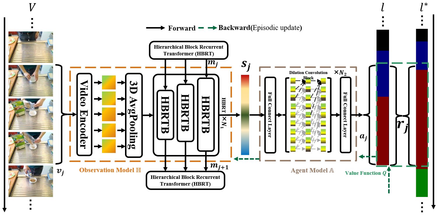
Figure 1: Overview of SVTAS-RL. To train the SVTAS-RL model, we first sample a video clip $v_{j}$, which is then parsed by the observation model $\mathbb{H}$ to yield the current state $s_{j}$. Subsequently, the agent $\mathbb{A}$ makes a decision $a_{j}$ based on the current state $s_{j}$, and the decision is evaluated by $Q$ to obtain a reward $r_{j}$.

3.1 Architecture

Task Definition: We regard a video $V\in\{x_{i}|i=0,\cdots,T-1\}$ as an ordered collection of image frames $x_{i}$, where $T$ denotes the total number of frames in the video. Each frame is assigned a corresponding label, denoted as $l_{i}^{*}\in\{0,\cdots,C-1\}$, where $C$ represents the total number of labels. The model’s predicted result is denoted by $l_{i}\in\{0,\cdots,C-1\}$. For SFTAS task, We perform non-overlapping stream sampling of the feature. For SVTAS task, We perform non-overlapping stream sampling of the video frame to ensure its efficient processing. After sampling, a feature clip or video clip $V_{j}$ will be fed into model to yield segment result $[l_{j\cdot L},\cdots,l_{j\cdot L+L}]$, where $j=0,\cdots,\lceil\frac{T}{L}\rceil$ and $L$ is the length of clip. Repeat the process and collect the results in each iteration until the end of the video. To model the task as a sequential decision-making problem, we define features of video clip as a state $s_{j}$. Accordingly, we define segment result of $V_{j}$ as an action $a_{j}=[l_{j\cdot L},\cdots,l_{j\cdot L+L}]$ and the action space is $a_{j}\in\mathbb{R}^{C\times L}$. Specifically, the agent model is defined as $\mathbb{A}(s_{j};\theta)$, the observation model as $\mathbb{H}(v_{j},m_{j};\phi)$, and the value function as $Q(a^{*}_{j},a_{j})$, where $m_{j}$ is the historical information about the observation.

3.1.1 Observation Model

As shown in Fig.1, the observation model $\mathbb{H}$, parameterized by $\phi$, observes a video clip at each time step. It encodes the video clip into a feature state $s_{j}$ and provides this as input to the agent model. Importantly, given the high degree of video information redundancy, we leverage two common pre-processing techniques in RL and video understanding, namely frame stacking [55] and frame skipping [34], to select an appropriate video clip $v_{j}$ length as a state $s_{j}$, which we formalize as $v_{j}\in\{[x_{j},x_{j+p},\cdots,x_{j+L}]\}$, $L=k\times p$, where $k$ is the number of stacked frames, $p$ is the number of skipped frames, $L$ is the length of video clip. To extract rich information from video clip, we have employed the video swin transformer [30], an action recognition model, as Video Encoder (VE) to observe the current video clip, and HBRT which inspired by Block-Recurrent Transformers [17] (BRT) to memorize history information and fuse the current video clip information. Notably, HBRT can be used as a model for SFTAS.

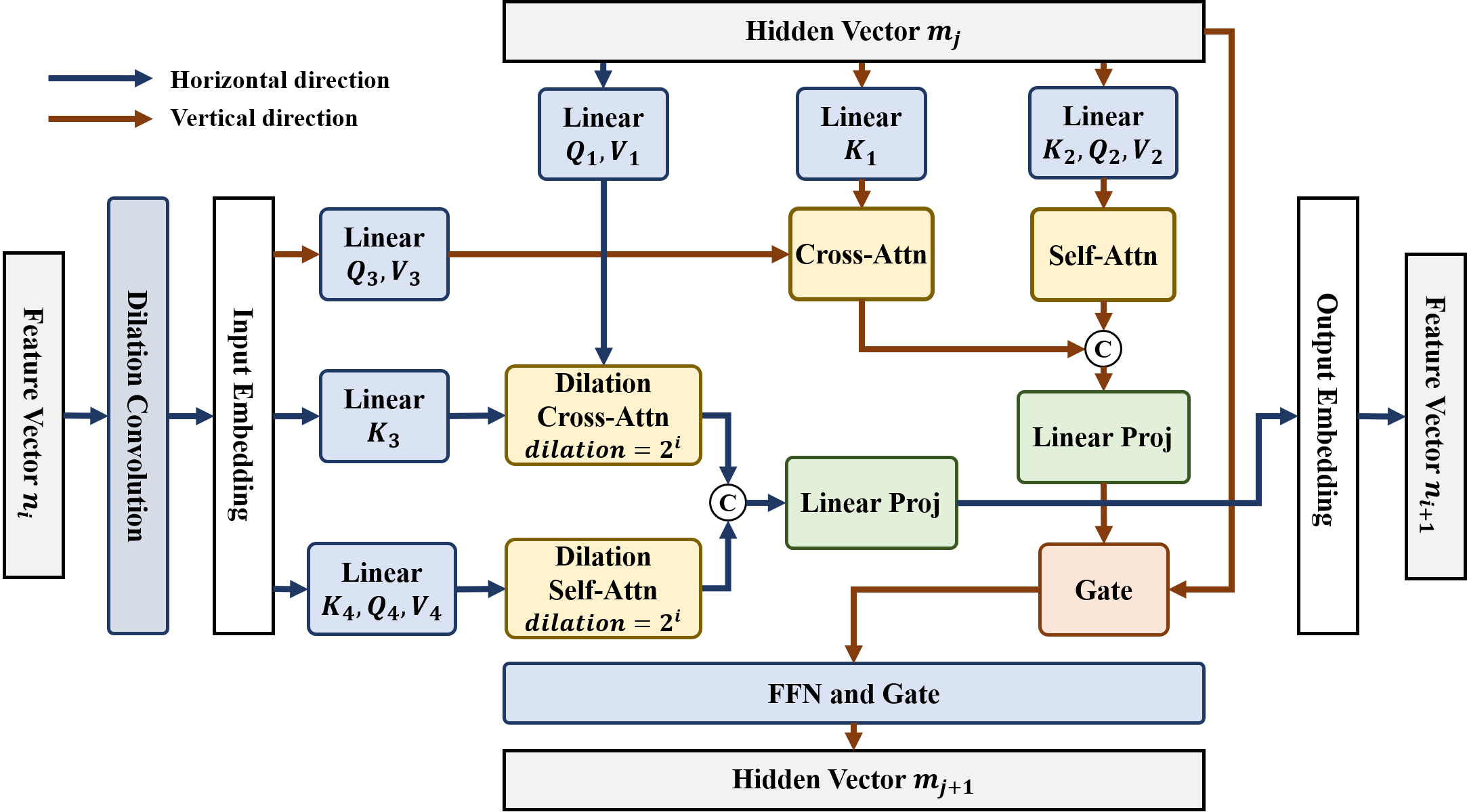
Figure 2: Overview of Hierarchical Block Recurrent Transformer (HBRT).

Hierarchical Block Recurrent Transformer

The HBRT architecture, illustrated in Fig.2, receives the output of VE $f_{j}$ and historical information $m_{j}\in\mathbb{R}^{D\times M}$ as input, and produces the state $s_{j}$ and updated historical information $m_{j+1}\in\mathbb{R}^{D\times M}$ as output, where $D$ is the dimension of information and $M$ is the length of information. Before feeding $f_{j}$ into HBRT, we compress its spatial information, retaining only temporal information, as the SVTAS task focuses on temporal modeling. The compressed feature $f_{j}^{t}$ will feed into $N_{1}$ hierarchical block Recurrent transformer block (HBRTB). Each HBRTB layer is consist of an dilated convolution, a BRT block with an dilated window mask, a feed-forward neural network and a gate neural network. The dilation rate of layer $o$ is set to $2^{o}$. The dilated convolution smooths the input feature $f_{j}^{t}$ [11], while the feed-forward neural network improves the feature expression ability of the model. Gate neural network consist of activation functions and linear layers for selective memory and updating of historical information. Horizontal direction represents the current information flow, while its vertical direction represents the historical information flow in HBRT. In addition, unlike BRT, which uses state IDs and position bias, we employ rotated relative position encoding [42] for each attention operation. Inspired by hierarchical representation design in ASformer [52], we modify hierarchical block attention operation of ASformer to a memory-friendly attention operation with dilated window mask. This modification not only enables the model to be trained on multiple samples but also improves its inference speed. Each layer’s representation in HBRT is passed to its corresponding layer in next state, instead of BRT that only passed to the last layer or the last layer’s preceding layer. This approach facilitates interaction of historical information when aggregating SVTAS features.

3.1.2 Agent Model

The agent model $\mathbb{A}$, parameterized by $\theta$, makes a decision $a_{j}$ based on current state $s_{j}$. As shown in Fig.1, the agent model is consist of a full-connect layer and $N_{2}$ dilated convolution blocks [11] which refine the result from full-connect layer. When evaluating the performance of the model, we will collect the decision $a_{j}$ made by the agent $\mathbb{A}$ and concatenate all the segmentation results from $a_{0}$ to $a_{\lceil\frac{T}{L}\rceil}$ in temporal order. Finally, evaluation indicators consistent with TAS tasks are adopted to ensure the substitution of SVTAS for TAS.

3.1.3 Reward

An RL reward measures the value of decision $a_{j}$ which made by agent $\mathbb{A}$. In the SVTAS-RL model, this refers to the integrity of the action segment in the single-step decision of agent. We use a value function based on the dice coefficient [33] as a reward to measure it. The formula is as follows:

$$r_{j}=\beta_{1}^{\frac{1}{C}\sum_{c=0}^{C-1}\frac{2|a_{j,c}\cap a_{j,c}^{*}|}{|a_{j,c}|\cup|a_{j,c}^{*}|}}+\beta_{2}=\beta_{1}^{\frac{1}{C}\sum_{c=1}^{C-1}\frac{2\sum_{i=j\cdot L}^{j\cdot L+k\cdot p}y_{i,c}p_{i,c}}{\sum_{i=j\cdot L}^{j\cdot L+k\cdot p}(y_{i,c}+p_{i,c})}}+\beta_{2}$$ (1)

where, $y_{i,c}$ represents the one-hot vector for class $c$ actions of frame $i$; $p_{i,c}$ represents the predicted probability from model for class $c$ actions of frame $i$; $\beta_{1}$ and $\beta_{2}$ is hyper-parameter.

3.2 Learning

1

input : Agent model $\mathbb{A}(\cdot;\theta)$, Environment model $\mathbb{H}(\cdot,\cdot;\phi)$, Historical information $m_{0}$, Learning rate $\alpha$, Frame-skipping $p$, Frame-stacking $k$, Video set $V$

output : Sequence of action labels for each frame of untrimmed video, $[l_{0},l_{1},\cdots,l_{T}]$

2 Initial $\mathbb{A}(\cdot;\theta)$, $\mathbb{H}(\cdot,\cdot;\phi)$, $m_{0}$, result list $list$ ;

3 for $n\leftarrow 0$ to $|V|$ do

4       Sample $V_{n}$ from video set $V$;

5       for $j\leftarrow 0$ to $\lceil\frac{|V_{n}|}{k\times p}\rceil$ do

6             Sample $I_{j}=[x_{j*L},\cdots,x_{j*L+k*p}]$ and $a_{j}^{*}=[l_{j*L},\cdots,l_{j*L+k*p}]$ from Video $V_{n}$;

7             $s_{j},m_{j+1}\leftarrow\mathbb{H}(I_{j},m_{j};\phi)$;

8             $a_{j}\leftarrow\mathbb{A}(s_{j};\theta)$;

9             $r_{j}\leftarrow Q(a^{*}_{j},a_{j})$;

10             $list.append(a_{j})$;

11            

12       end for

13      $\mathbf{J}(\theta,\phi)=\mathbb{E}_{p_{\theta,\phi}(a0:\lceil\frac{|V_{n}|}{k\times p}\rceil)}[\sum_{j=0}^{\lceil\frac{|V_{n}|}{k\times p}\rceil}r_{j}]$;

       /* $P(\cdot|I_{j},\theta,\alpha)$ is the distribution probability of $l_{i,c}$ */

14       $\nabla_{\theta,\phi}\mathbf{J}(\theta,\phi)=\frac{1}{q}\sum_{j=0}^{q}r_{j}\nabla_{\theta,\alpha}CrossEntropy(a_{j},a_{j}^{*})$;

15       $\{\theta,\phi\}\leftarrow\{\theta,\phi\}-\alpha\nabla_{\theta,\phi}\mathbf{J}(\theta,\phi)$;

16      

17 end for

Algorithm 1 Monte Carlo Episodic REINFORCE Learning for SVTAS task (MC)

The optimal action trajectory of a video is actually deterministic in our sequential decision-making task, which is denoted as $A^{*}=[a_{0}^{*},a_{1}^{*},\cdots,a_{q}]$, where $q=\lceil\frac{|V_{n}|}{k\times p}\rceil$. The optimization objective of the model is to maximize the accumulated rewards from each decision. The strategy learning methods for RL based on update methods are divided into temporal difference update and Monte Carlo update. So, we also designed two strategy learning methods, they are: Monte Carlo update learning method based on REINFORCE algorithm and temporal difference update learning method based on actor-critic algorithm. In RL tasks to maximize expectations, parameter updates typically use gradient ascent, while in computer vision tasks to minimize losses, parameter updates typically use gradient descent. In the SVTAS task, two parameter update algorithms that we designed using the same gradient descent algorithm as most computer vision tasks. Formula reasoning for gradient estimation can be found in the Appendix.

3.2.1 Monte Carlo Update

The Monte Carlo updated method usually uses the REINFORCE algorithm [50]. However, the original REINFORCE algorithm is updated using gradient ascent, so we modify the REINFORCE algorithm for the SVTAS task, following DSN [56]. In our MC algorithm Algorithm.1, we use an approximate approach to estimate expectations. From an optimization perspective, the value function can be thought of as a variable coefficient that indicates how much confidence there is that the current gradient direction is the globally optimal gradient direction.

1

input : Agent model $\mathbb{A}(\cdot;\theta)$, Environment model $\mathbb{H}(\cdot,\cdot;\phi)$, Historical information $m_{0}$, Learning rate $\alpha$, Frame-skipping $p$, Frame-stacking $k$, Video set $V$

output : Sequence of action labels for each frame of untrimmed video, $[l_{0},l_{1},\cdots,l_{T}]$

2 Initial $\mathbb{A}(\cdot;\theta)$, $\mathbb{H}(\cdot,\cdot;\phi)$, $m_{0}$, result list $list$ ;

3 for $n\leftarrow 0$ to $|V|$ do

4       Sample $V_{n}$ from video set $V$;

5       for $j\leftarrow 0$ to $\lceil\frac{|V_{n}|}{k\times p}\rceil$ do

6             Sample $I_{j}=[x_{j*L},\cdots,x_{j*L+k*p}]$ and $a_{j}^{*}=[l_{j*L},\cdots,l_{j*L+k*p}]$ from Video $V_{n}$;

7             $s_{j},m_{j+1}\leftarrow\mathbb{H}(I_{j},m_{j};\phi)$;

8             $a_{j}\leftarrow\mathbb{A}(s_{j};\theta)$;

9             $r_{j}\leftarrow Q(a^{*}_{j},a_{j})$;

10             $list.append(a_{j})$;

11             $\mathbf{J}(\theta,\phi)=r_{j}$;

12             $\nabla_{\theta,\phi}\mathbf{J}(\theta,\phi)=r_{j}\nabla_{\theta,\alpha}CrossEntropy(a_{j},a_{j}^{*})$;

13             $\{\theta,\phi\}\leftarrow\{\theta,\phi\}-\alpha\nabla_{\theta,\phi}\mathbf{J}(\theta,\phi)$;

14            

15       end for

16      

17 end for

Algorithm 2 Temporal Difference Actor-Critic Learning for SVTAS task (TD)

3.2.2 Temporal Difference Update

The actor-critic algorithm [43] is a common algorithm for the temporal difference updated method. As with the original REINFORCE algorithm, we also modify it to a gradient descent version Algorithm.2, and since our critic model can be estimated directly by the algorithm without bias, we only need to update the parameters of the agent in a single step. Note that we directly use the reward here as the error of the temporal difference, which is crude, but also allows the model to be optimized roughly toward the optimization objective of the SVTAS task.

4 Experiment and Discussion

4.1 Datasets and Evaluation Metrics

Datesets: The GTEA [12] dataset contains 28 videos corresponding to 7 different activities, performed by 4 subjects. On average, there are 20 action instances per video. The evaluation was performed by excluding one subject to use cross-validation. The 50Salads [41] dataset contains 50 videos with 17 action classes. On average, each video contains 20 action instances. 50Salads also uses five-fold cross-validation. The Braekfast [20] dataset is the largest of the four datasets. In total, Braekfast contains 77 hours of 1712 videos. It contains 48 different actions, and each video contains an average of 6 action instances. Also, it will be evaluated by four-fold cross-validation. The EGTEA [26] dataset has the longest average video length in the four datasets. In total, EGTEA contains 28 hours of cooking activities from 86 unique sessions of 32 subjects. It contains 20 different actions, and each video contains an average of 45 action instances. Also, it will be evaluated by three-fold cross-validation.

Metrics: To evaluate SVTAS task results, we adopt several metrics including frame-wise accuracy (Acc) [11], segmental edit distance (Edit) [11], and the F1 score at temporal IoU threshold 0.1, 0.25, 0.5 (denote by F1@{0.1, 0.25, 0.5}, [24]. F1 score is proposed to measure the integrity of action segment and F1@0.5 is the most important indicator for TAS. Edit score is measure the action sequence distance between the inferred result and the ground true. The frame-wise accuracy is measure quality of single-frame classification.

4.2 Implementation Details

We adopt AdamW optimizer and the base learning rate of $5\times 10^{-4}$ with a $1\times 10^{-4}$ weight decay. The spatial resolution of the input video is $224\times 224$. We use Kinetics-600 [5] pre-trained weight for all feature extractors. The $k$x$p$ for GTEA is 64x2, for 50Salads, Breakfast and EGTEA is 128x8. The model is trained 80 epochs with batch size is set to 1 for GTEA and 50Salads and trained 50 epochs with batch size is set to 1 for Breakfast and EGTEA. $\beta_{1}$ is 4 and $\beta_{2}$ is -1. $D$ is set to 128 and $M$ is set to 512. More details of the experiment can be obtained from Appendix.

4.3 Impact of TAS migration to STAS

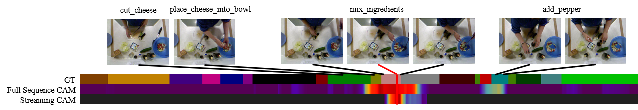
Figure 3: The importance of global contextual information. Class Activation Map (CAM) for red frame in full sequence TAS and SFTAS. Streaming CAM is mostly black because the frames are not available at inference time.

In Tab.1, we observe that migrating TAS models to STAS generates huge performance gap, and even HBRT designed for streaming data still cannot fill the performance gap, which indicates that changing TAS into STAS is a challenging task. A closer look reveals that optical flow modality with temporal information play an important role in TAS, but to achieve end-to-end segmentation we will only use rgb modality, which makes the end-to-end STAS more challenging.

	Model	paradigm	modality	Acc	Edit	F1@{0.1,0.25,0.5}
full	ASformer	sequence	rgb feature	56.3	63.2	63.6	56.5	41.2
	ASformer	sequence	rgb+flow feature	73.5	75.0	76.0	70.6	57.4
streaming	ASformer	sequence	rgb+flow feature	52.7	57.2	51.3	51.3	37.7
	HBRT	sequence	rgb feature	49.3	56.4	55.6	48.9	34.6
	HBRT	sequence	flow feature	61.8	65.3	66.5	60.9	47.6
	HBRT	sequence	rgb+flow feature	62.9	67.9	68.1	62.7	48.7
	SVTAS	cluster	rgb	65.6	70.9	71.3	64.9	49.8

Table 1: Migration experiment from TAS to STAS in Breakfast. †means migration experiment.

Fig.3 shows that in full sequence TAS, global contextual information is required. However, in streaming scenario, the model will rely entirely on the information of the current video clip, which inspires us to regard STAS as a clustering task rather than a sequence-to-sequence transformation task that need to observe full sequence information. As can be seen in Fig.4, TAS uses single-frame features extracted through a sliding window, which is a tangled line in the feature manifold. It is suitable for sequence-to-sequence transformation task. SVTAS without global contextual information should be seen as a clustering task and should not use former features. So, SFTAS performs poorly. And, as shown in Tab.6 Line.2-Line.5, when switching to the clustering paradigm, it can significantly improve the model performance. So, STAS should be treated as a clustering task.

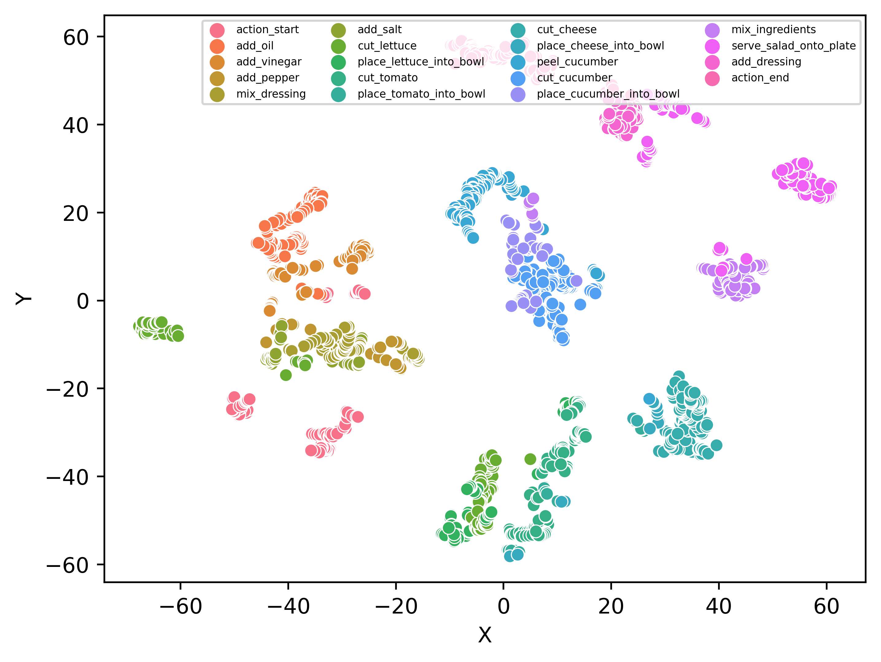
(a) RGB

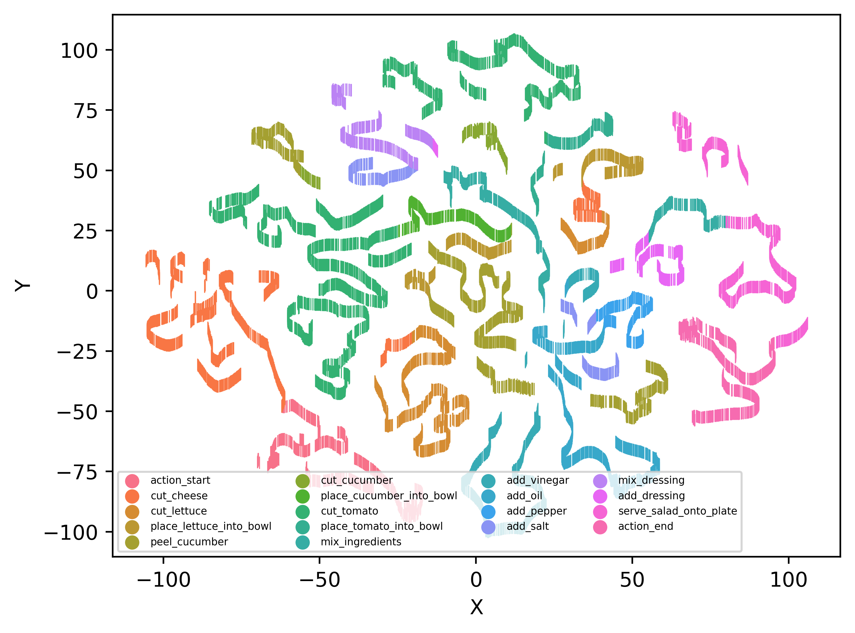
(b) TAS Input

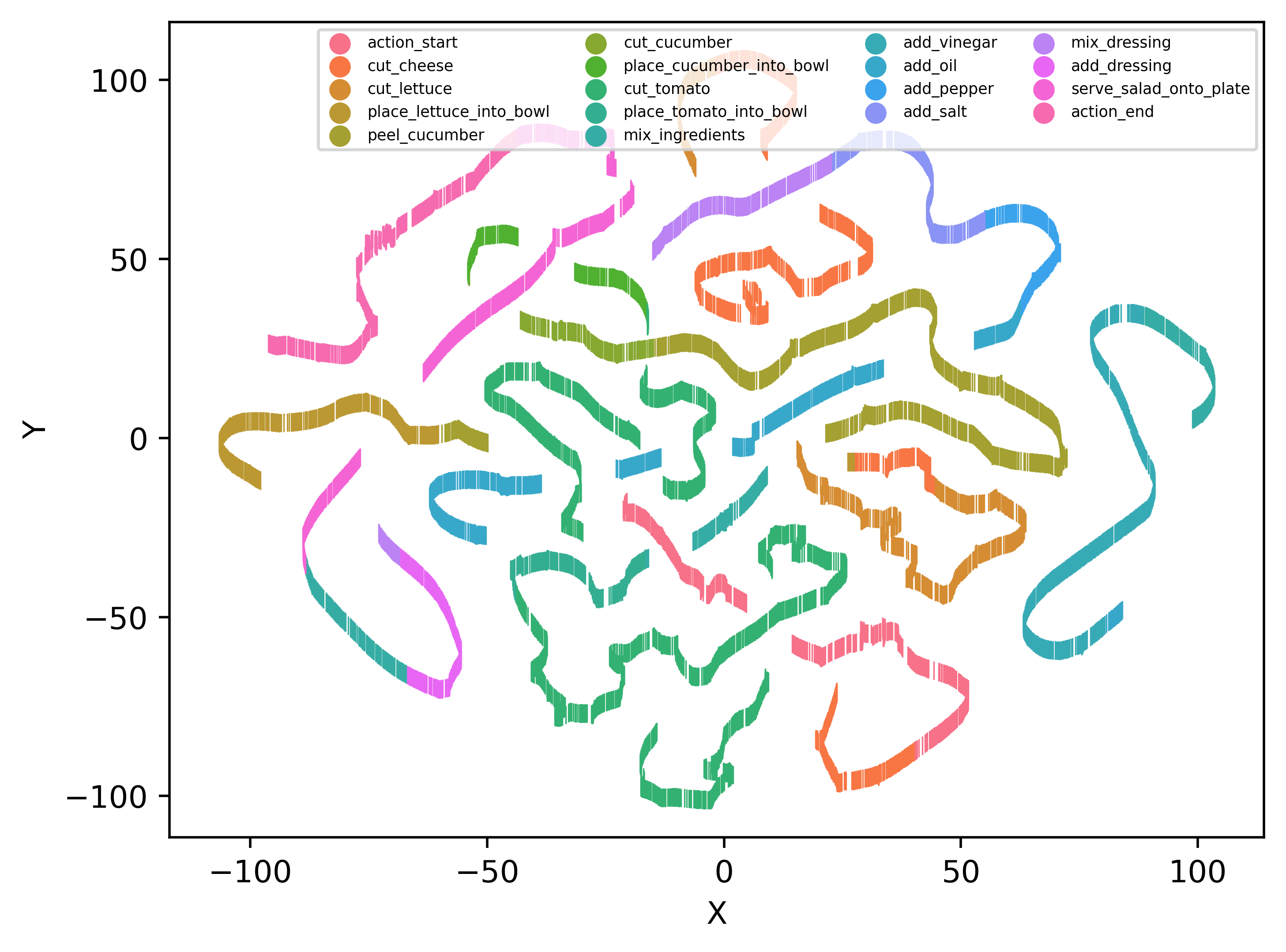
(c) TAS Output

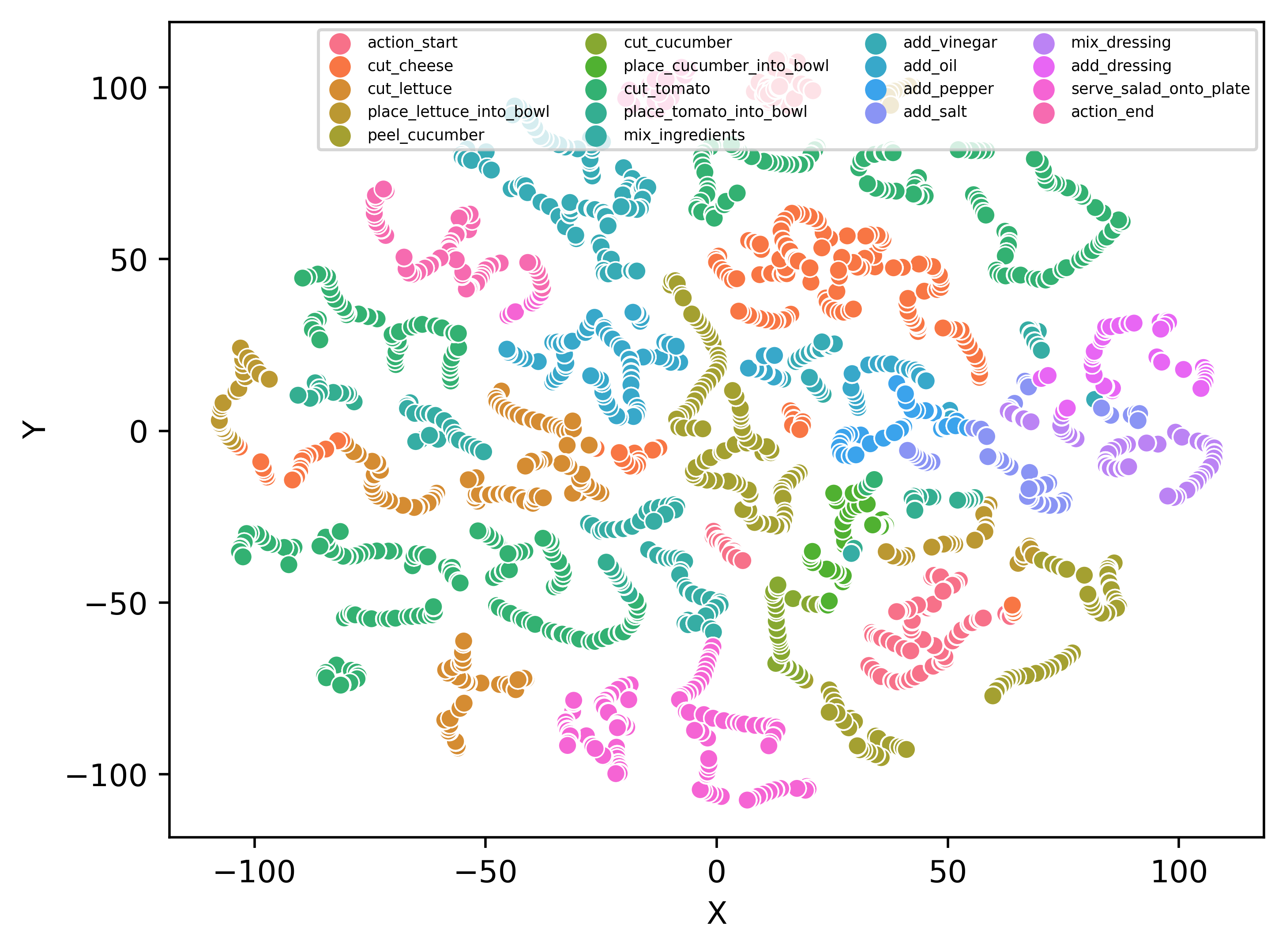
(d) SVTAS Input

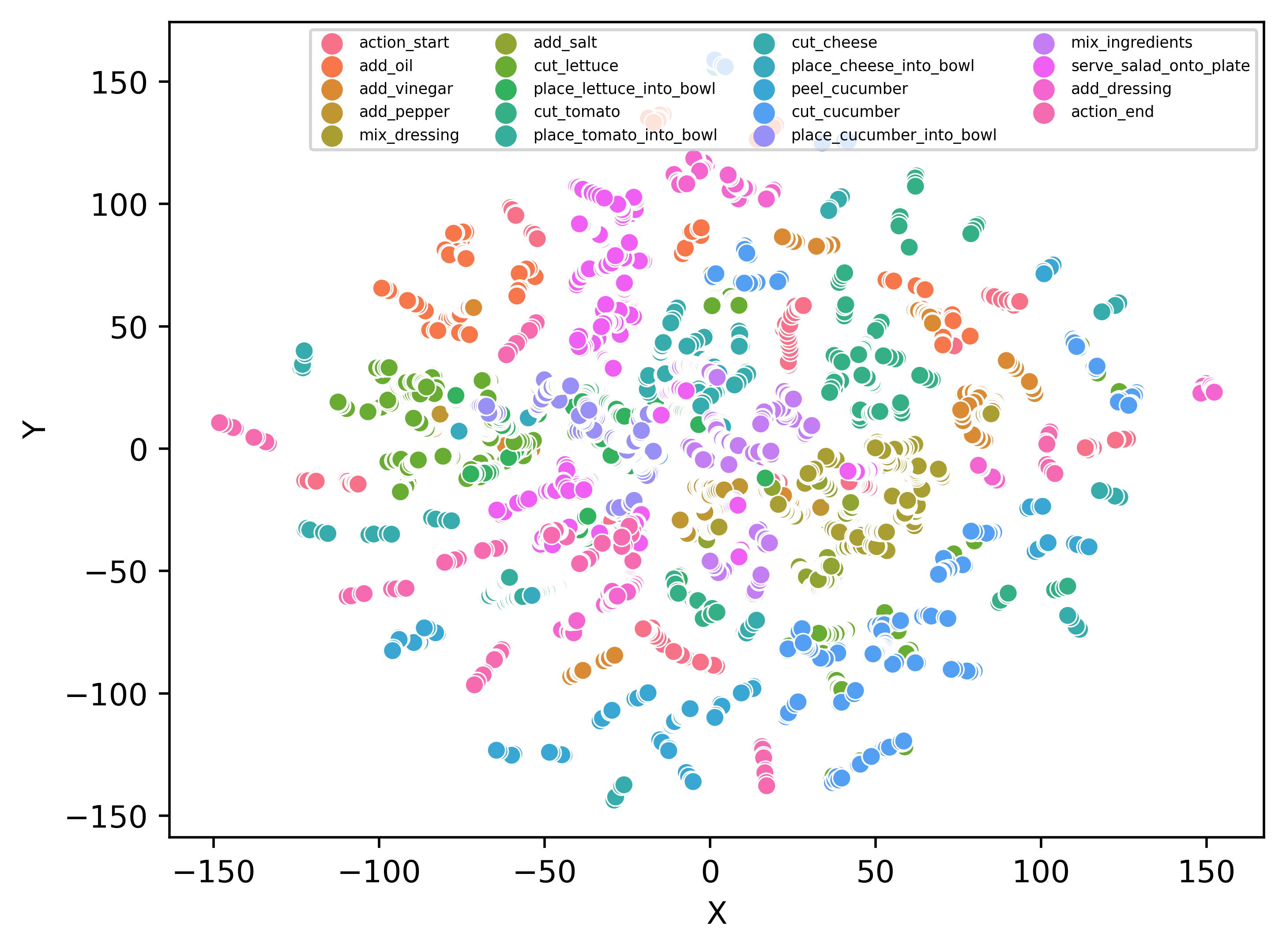
(e) SVTAS Output

Figure 4: Comparison of feature manifold. All features are visualized by t-SNE. Obviously, TAS is a sequence-to-sequence transformation task and SVTAS is a clustering task.

Comparison between end-to-end training and training separately.

We consider two approaches of clustering in SVTAS, single frame clustering approach and action segment clustering approach. The single frame clustering approach like an image classification model that only clusters each video frame, while action segment clustering approach will model temporal information to cluster the action segment after video encoding. From Tab.6 Line.6-Line.9, we can find that the action segment clustering approach is significantly better than the single frame clustering approach. Similar to TAS, training separately is possible for VE and temporal models, Line.8 vs Line.9 in Tab.6 shows that end-to-end training is better than training separately. We think it is because that end-to-end training reduces the error propagation rate more effective. We define the error propagation rate to be calculated as the number of samples segmented incorrectly by both submodels compared to the number of samples segmented incorrectly in the final submodel. We also define the correction capability of the models, which is calculated as the number of samples that are incorrect in the first submodule but are corrected in the second submodule compared to the number of samples that segment correctly in the final submodel. As can be observed in Fig.6, the correction capability of model is similar, but the end-to-end training one has a lower error propagation rate which indicates end-to-end training can optimize globally.

	manifold	Model	Acc	Edit	F1@{0.1,0.25,0.5}
sep	sequence feature	FC	52.0	4.7	6.0	4.0	1.9
		ASformer	60.8	43.4	50.7	46.6	40.4
	clustering feature	FC	78.5	17.4	26.2	22.8	16.6
		ASformer	85.8	69.3	78.0	76.0	68.5
e2e	single frame cluster	VE†+FC	81.1	50.1	63.0	59.1	50.1
		VE+FC	82.6	60.7	66.7	64.4	54.9
sep	action segment cluster	SVTAS	84.4	75.4	83.6	82.7	72.9
e2e		SVTAS	85.1	76.0	83.9	82.5	74.4

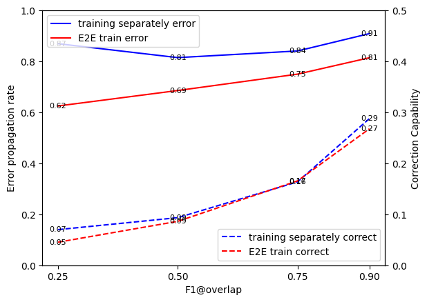
Figure 5: Comparison of training method and feature manifold on STAS in split1 of 50Salads. sep means training separately. e2e means end-to-end training. †means pre-trained VE from an end-to-end SVTAS. FC means full connect layer.

[]

Figure 6: Analysis of propagation of error and correction capabilities between training separately and end-to-end training. End-to-end training reduces propagation of error.

Nonconformity between optimization objective and optimization direction.

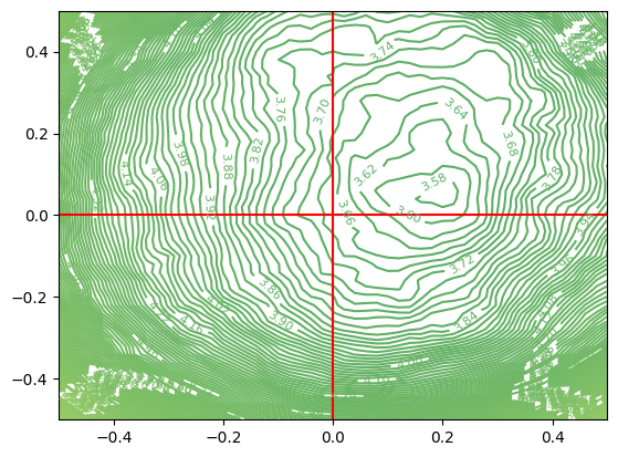
(a) TAS

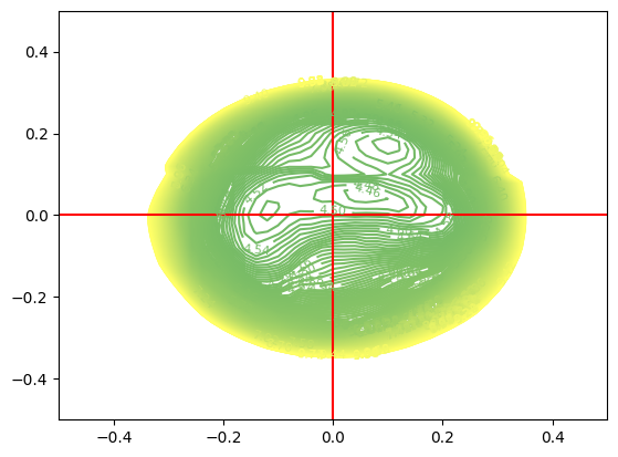
(b) SVTAS

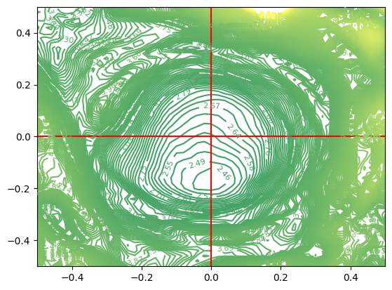
(c) SVTAS-RL(TD)

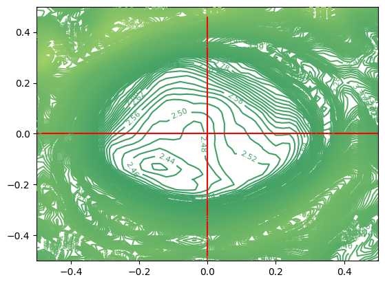
(d) SVTAS-RL(MC)

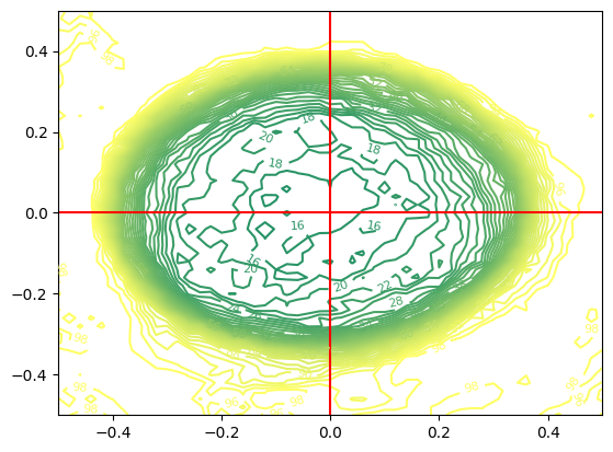
(e) F1@0.50 Error

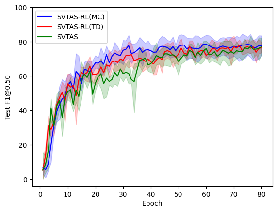
(f) GTEA

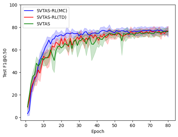
(g) 50Salads

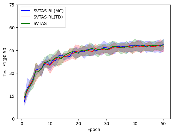
(h) Breakfast

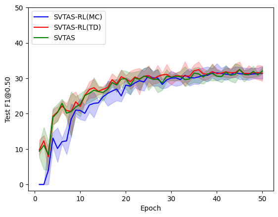
(i) EGTEA

Figure 7: Visualize optimization objective and optimization direction by 2D surface. (a)-(d) are optimization direction surface. (e) is optimization objective surface. (f)-(i) is training state.

Fig.7 (e) shows that (0, 0) is the center of the optimization objective. The optimization direction surfaces of models all have different degrees offset to the optimization objective center, which means that neither the previous nor our proposed method can unify the optimization objective and the optimization direction. However, method with RL we proposed can maintain convexity near the center of the optimization objective, enabling the model to achieve a global optimum in the optimization direction. The optimization surface of the model without RL has many local optima that are difficult to optimize. Fig.7 (f)-(i) proves that the optimization method with RL we proposed can update the model parameters faster and better during the training process.

		Dataset	GTEA					50Salads					Berakfast					EGTEA
		Metric	Acc	Edit	F1@{0.1,0.25,0.5}			Acc	Edit	F1@{0.1,0.25,0.5}			Acc	Edit	F1@{0.1,0.25,0.5}			Acc	Edit	F1@{0.1,0.25,0.5}
full (rgb + flow feature)		Bi-LSTM [39]	55.5	-	66.5	59.0	43.6	55.7	55.6	62.6	58.3	47.0	-	-	-	-	-	70	28.5	27	23.1	15.1
		Dilated TCN [21]	58.3	-	58.8	52.2	42.2	59.3	43.1	52.2	47.6	37.4	-	-	-	-	-	-	-	-	-	-
		ST-CNN [22]	60.6	-	58.7	54.4	41.9	59.4	45.9	55.9	49.6	37.1	-	-	-	-	-	-	-	-	-	-
		ED-TCN [21]	64.0	-	72.2	69.3	56.0	64.7	52.6	68.0	63.9	52.6	43.3	-	-	-	-	70.1	28.6	31.1	27.7	19.6
		TDRN [23]	70.1	74.1	79.2	74.4	62.7	68.1	66.0	72.9	68.5	57.2	-	-	-	-	-	-	-	-	-	-
		MS-TCN [11]	76.3	79.0	85.8	83.4	69.8	80.7	67.9	76.3	74.0	64.5	66.3	61.7	52.6	48.1	37.9	69.2	32.2	32.1	28.3	18.9
		MS-TCN++ [25]	80.1	83.5	88.8	85.7	76.0	83.7	74.3	80.7	78.5	70.1	67.6	65.6	64.1	58.6	45.9	-	-	-	-	-
		BCN [49]	79.8	84.4	88.5	87.1	77.3	84.4	74.3	82.3	81.3	74.0	70.4	66.2	68.7	65.5	55.0	-	-	-	-	-
		Global2Local [13]	78.5	84.6	89.9	87.3	75.8	82.2	73.4	80.3	78.0	69.8	70.7	73.3	74.9	69.0	55.2	-	-	-	-	-
		ASRF [18]	77.3	83.7	89.4	87.8	79.8	84.5	79.3	84.9	83.5	77.3	67.6	72.4	74.3	68.9	56.1	-	-	-	-	-
		C2F-TCN [40]	80.8	86.4	90.3	88.8	77.7	84.9	76.4	84.3	81.8	72.6	76.0	69.6	72.2	68.7	57.6	-	-	-	-	-
		ASFormer [52]	79.7	84.6	90.1	88.8	79.2	85.6	79.6	85.1	83.4	76.0	73.5	75.0	76.0	70.6	57.4	-	-	-	-	-
		m-GRU+GTRM [16]	-	-	-	-	-	-	-	-	-	-	-	-	-	-	-	69.5	41.8	41.6	37.5	25.9
		bridge-prompt [24]	81.2	91.6	94.1	92.0	83.0	88.1	83.8	89.2	87.8	81.3	-	-	-	-	-	-	-	-	-	-
		UVAST [2]	80.2	92.1	92.7	91.3	81.0	87.4	83.9	89.1	87.6	81.7	77.1	69.7	76.9	71.5	58.0	-	-	-	-	-
streaming	feature	IDT+LM [36]	-	-	-	-	-	48.7	45.8	44.4	38.9	27.8	-	-	-	-	-	-	-	-	-	-
		ASformer [52] †	76.3	79.7	85.4	83.1	72.8	70.0	54.0	62.1	57.6	49.1	52.7	57.2	57.7	51.3	37.7	-	-	-	-	-
		HBRT(ours)	74.9	78.7	84.3	82.2	72.5	74.2	56.2	63.7	60.4	52.1	62.9	67.9	68.1	62.7	48.7	-	-	-	-	-
	video(rgb)	ETSN [19]	78.3	79.9	87.1	84.5	71.8	83.1	71.1	79.0	76.8	69.5	-	-	-	-	-	-	-	-	-	-
		SVTAS(ours)	79.3	82.7	87.1	86.4	79.1	86.7	78.4	85.3	83.7	77.2	65.6	70.9	71.3	64.9	49.8	69.6	47.3	50.1	46.0	32.8
		SVTAS-RL(TD)(ours)	78.9	86.4	90.9	88.7	80.0	87.4	79.8	86.1	85.0	79.6	64.9	70.6	71.3	65.0	49.4	69.7	47.9	51.2	46.9	32.8
		SVTAS-RL(MC)(ours)	78.8	86.4	90.0	88.4	81.1	87.3	78.9	85.9	84.2	80.1	63.7	70.1	70.5	64.3	49.6	68.8	47.4	49.8	45.4	32.2

Table 2: Comparison with the state-of-the-art results on four datasets. Global action segment integrity was measured by F1 metrics. Bold and underlined denote the best and second-best results in each column, respectively. †means migration experiment. Feature means rgb + flow (optical flow) features, so it is unfair comparison when across horizontal line. But we only use rgb modality to achieve comparable results of the full sequence by end-to-end streaming method.

4.4 Comparison to prior work

We show in Tab.2 the comparison results of three segmentation paradigms: TAS, SFTAS, and SVTAS. We can observe that the end-to-end SVTAS approaches are already very comparable to the SOTA model of the current TAS model. And our method even outperforms the latter on the dataset EGTEA, which indicates that the stream-based approach is better than latter for ultra-long videos action segmentation. Although the SVTAS-RL(MC) approach is lower than the SVTAS-RL(TD) on F1@0.1 and F1@0.25, the former performs better on F1@0.5. Just as the metric in object detection uses an IOU threshold of 0.5 as a more important benchmark for comparison, indicating that the former model is more accurate in integrity of action segment through guidance from RL reward. In Tab.2, Breakfast does not perform as expected. We believe that this is caused by the poor quality of the rgb modality for Breakfast dataset. More details of the comparison between datasets can be obtained from the Appendix. From Tab.6, we can see that optical flow modality is crucial to Breakfast. And our proposed method already outperform the full sequence TAS model when using the same rgb modality.

4.5 Ablation Study

Avg.$T$	Dataset	$k$ x $p$	Acc	Edit	F1@{0.1,0.25,0.5}
1115.2	GTEA	16 x 2	75.2	69.7	79.7	75.7	67.7
		32 x 2	77.8	80.6	84.4	81.0	72.7
		64 x 2	79.9	85.6	88.0	86.5	79.3
		128 x 2	79.2	85.7	87.7	84.8	78.1
11551.9	50Salads	128 x 2	84.1	60.2	67.9	65.8	57.4
		128 x 4	84.6	70.8	79.0	75.6	69.6
		128 x 8	85.7	75.7	83.6	82.3	76.4
		128 x 12	85.3	77.4	85.8	84.3	75.7
2097.5	Breakfast	32 x 32	57.8	62.5	64.1	58.6	37.2
		64 x 16	62.1	65.9	66.5	60.8	44.6
		128 x 8	63.2	68.8	68.7	63.2	47.4
		256 x 4	64.3	66.8	68.7	63.5	49.7

Table 3: Avg.$T$ means average number of frames per video.

The experiments in Tab.3 are all on split1 and EGTEA Avg.$T$ is 28157.7. From Tab.3 we can observe that there are three principles for the selection of $k$ and $p$: (a) The larger $k$ is in a certain range, the better. However, due to hardware limitations, $k$ cannot be infinite. Fortunately beyond a certain value, the marginal gain in model performance will decrease. This threshold value is related to the characteristic of a particular dataset. (b) The selection of $p$ is related to the current dataset and its effect is not as significant as $k$. (c) The combination of $k$ and $p$ is related to the average number of frames per video in the current dataset. Overall, there exists a range where the larger the time step is, the better, but once this threshold is exceeded, the integrity of action segment of the model will decrease.

model	pass	Acc	Edit	F1@{0.1,0.25,0.5}
horizontal attn	-	74.1	75.6	82.9	81.4	69.6
+ vertical attn	-2	74.5	79.7	83.7	81.3	71.0
HBRT	all	74.9	78.7	84.3	82.2	72.5

Table 4: vertical and horizontal direction ablation experiments about HBRT in the feature modality of GTEA with HBRT. -2 means only pass last but not least layer memory to next state.

Tab.4 shows the ablation experiments on the HBRT structure. We can observe that the addition of memory information in the vertical direction enhances the Edit score. This indicates that the network is able to model past action information through the extraction and updating of memory information. And it enhances the model’s ability to infer sequential actions. Line.4 show that HBRT can enhance integrity of action segment through the passing hierarchical memory information.

5 Conclusion

In the paper, we propose SVTAS-RL which can broaden the application scenario of TAS and introducing the training method of RL. Extensive experiments have shown that STAS, as an important complementary task to TAS, has promising applications for processing long videos. Although our model still has a little bit latency when inferring, we believe that through our inspiration, the academic community will further explore to achieve real-time action segmentation.

Appendix A Appendix

A.1 Hyper-parameter Tables

The specific parameter settings on the GTEA, 50Salads, Breakfast and EGTEA datasets in this paper are shown in Tab.5 to 8.

Dateset	GTEA
Modality	rgb(MC)	rgb(TD)	rgb+flow feature
Epochs	80	80	80
Batch Size	1	1	1
Seed	0	0	0
Frame Stacking	64	64	64
Frame Skipping	2	2	2
Video Encoder	Swin3D	Swin3D	-
Pretrained wieght	kinetics 600	kinetics 600	-
Need SBP [7]	$\times$	$\times$	$\times$
Image Size	224	224	-
M	512	512	512
optimizer	AdamW	AdamW	AdamW
learning rate	0.0005	0.0005	0.0005
finetuning scale factor	0.02	0.02	-
LR scheduler	CosineAnnealingLR	CosineAnnealingLR	CosineAnnealingLR
$\beta_{1}$	4	4	4
$\beta_{2}$	-1	-1	-1
$N_{1}$	8	8	8
$N_{2}$	3	3	3

Table 5: GTEA Hyper-parameter Table.

Dateset	50Salads
Modality	rgb(MC)	rgb(TD)	rgb+flow feature
Epochs	80	80	80
Batch Size	1	1	1
Seed	0	0	0
Frame Stacking	128	128	128
Frame Skipping	8	8	8
Video Encoder	Swin3D	Swin3D	-
Pretrained wieght	kinetics 600	kinetics 600	-
Need SBP [7]	✓	✓	$\times$
Image Size	224	224	-
M	512	512	512
optimizer	AdamW	AdamW	AdamW
learning rate	0.0005	0.0005	0.0005
finetuning scale factor	0.1	0.02	-
LR scheduler	CosineAnnealingLR	CosineAnnealingLR	CosineAnnealingLR
$\beta_{1}$	4	4	4
$\beta_{2}$	-1	-1	-1
$N_{1}$	8	8	8
$N_{2}$	3	3	3

Table 6: 50Salads Hyper-parameter Table.

Dateset	Breakfast
Modality	rgb(MC)	rgb(TD)	rgb+flow feature
Epochs	50	50	50
Batch Size	1	1	1
Seed	0	0	0
Frame Stacking	128	128	128
Frame Skipping	8	8	8
Video Encoder	Swin3D	Swin3D	-
Pretrained wieght	kinetics 600	kinetics 600	-
Need SBP [7]	✓	✓	$\times$
Image Size	224	224	-
M	512	512	512
optimizer	AdamW	AdamW	AdamW
learning rate	0.0001	0.0002	0.0001
finetuning scale factor	0.1	0.1	-
LR scheduler	CosineAnnealingLR	CosineAnnealingLR	CosineAnnealingLR
$\beta_{1}$	2	2	4
$\beta_{2}$	-0.5	0	-1
$N_{1}$	8	8	8
$N_{2}$	3	3	3

Table 7: Breakfast Hyper-parameter Table.

Dateset	EGTEA
Modality	rgb(MC)	rgb(TD)
Epochs	50	50
Batch Size	1	1
Seed	0	0
Frame Stacking	128	128
Frame Skipping	8	8
Video Encoder	Swin3D	Swin3D
Pretrained wieght	kinetics 600	kinetics 600
Need SBP [7]	✓	✓
Image Size	224	224
M	512	512
optimizer	AdamW	AdamW
learning rate	0.0005	0.0001
finetuning scale factor	0.1	0.1
LR scheduler	CosineAnnealingLR	CosineAnnealingLR
$\beta_{1}$	4	4
$\beta_{2}$	-0.5	-0.5
$N_{1}$	8	8
$N_{2}$	3	3

Table 8: EGTEA Hyper-parameter Table.

A.2 The Proof of Validity of Reinforce Learning

We will show that the descent gradient of the SVTAS can be estimated using reinforcement learning methods.

Symbol	Definition
$V$	video dataset
$T$	the length of video
$C$	number of action categories
$i$	image serial number, $i\in{0,\cdots T-1}$
$k$	frame-stacking number
$p$	frame-skipping number
$L$	the length of video clip
$q$	the max video clip serial number, $q=\lceil\frac{T}{k\times p}\rceil$
$j$	video clip serial number, $j\in{0,\cdots q}$
$I$	image sequence corresponding to one video
$I_{j}$	image sequence corresponding to $j$th video clip
$s_{j}$	state corresponding to $j$th video clip
$c$	the $c$th action
$l_{i,c}$	prediction probability of corresponding to $c$th action of $i$th image frame
$l^{*}_{i,c}$	one-hot label corresponding to $c$th action of $i$th image frame
$a_{j}$	prediction sequence corresponding to $j$th video clip
$a^{*}_{j}$	label sequence corresponding to $j$th video clip
$a$	prediction sequence corresponding to whole video
$a^{*}$	label sequence corresponding to whole video
$Q(\cdot,\cdot)$	reward value which directly measure action segment integrity of video
$\theta$	the parameters of STAS model (The paper breaks it down as $\theta$ and $\alpha$)
$P(\cdot|I_{j},\theta)$	the distribution of $a_{j}$, $a_{j}\sim P(\cdot|I_{j},\theta)$
$\pi_{\theta}(a_{j}|s_{j})$	the policy of the decision from model

Table 9: Symbol Definition Table.

The optimization objective of the STAS task is to maximize the action segment integrity of the entire video:

$$\mathbb{J}_{\theta}=\mathop{max}\limits_{\theta}\mathop{\mathbb{E}}\limits_{I\sim V}[\mathop{\mathbb{E}}\limits_{a_{j}\sim P(\cdot|I_{j},\theta)}(Q(a,a^{*}))]$$ (2)

Since optimizing the entire video dataset is not practical, we consider maximizing expectation for a single video:

$$\mathbb{J}_{\theta}=\mathop{max}\limits_{\theta}\mathop{\mathbb{E}}\limits_{a_{j}\sim P(\cdot|I_{j},\theta)}(Q(a,a^{*}))$$ (3)

A.2.1 The Proof of Invalidity of Supervised Learning for STAS task

The optimization objective function of the supervised learning is to minimize the classification loss of a single frame:

$$\mathop{min}\limits_{\theta}\mathbb{J}(\theta)=\mathop{min}\limits_{\theta}\frac{1}{q\times k\times C}\sum_{j=0}^{q}\sum_{i=j\cdot L}^{j\cdot L+k\cdot p}\sum_{c=0}^{C-1}l^{*}_{i,c}\log P(l_{i,c}|I_{j},\theta)$$ (4)

It obviously only indirectly optimizes the action segment integrity of the entire video.

A.2.2 The Proof of Validity of Monte Carlo Episodic REINFORCE Learning for SVTAS task

Our proof is consistent with [35]. Firstly, we define the optimization function equation from equation 3, here, we approximate $Q(a,a^{*})$ as $\sum_{j=0}^{q}Q(a_{j},a^{*}_{j})$:

$$\mathbb{J}_{\theta}=\mathop{max}\limits_{\theta}\mathop{\mathbb{E}}\limits_{a_{j}\sim P(\cdot|I_{j},\theta)}(\sum_{j=0}^{q}Q(a_{j},a^{*}_{j}))$$ (5)

Secondly, in order to use gradient descend algorithm to optimize parameters, we calculate the gradient of optimization function equation 5. Then apply log derivative trick for it[56].

$$\nabla_{\theta}\mathbb{J}(\theta)=\mathop{\mathbb{E}}\limits_{a_{j}\sim\pi_{\theta}(a_{j}|s_{j})}[\sum_{j=0}^{q}Q(a_{j},a^{*}_{j})\nabla_{\theta}\log\pi_{\theta}(a_{j}|s_{j})]$$ (6)

$$\approx\frac{1}{q}\sum_{j=0}^{q}Q(a_{j},a^{*}_{j})\nabla_{\theta}\log P(\cdot|I_{j},\theta)$$ (7)

Thirdly, since the probability space of $a_{j}$ is too large because of $a_{j}\in\mathbb{R}^{k\times C}$, and it’s hard to compute directly, we approximate $P(\cdot|I_{j},\theta)$ as $\frac{1}{k}\sum_{i=j\cdot L}^{j\cdot L+k\cdot p}P(l_{i,c}|I_{j},\theta)$, where $c$ is prediction action index. So:

$$\nabla_{\theta}\mathbb{J}(\theta)\approx\frac{1}{q}\sum_{j=0}^{q}Q(a_{j},a^{*}_{j})\frac{1}{k}\sum_{i=j\cdot L}^{j\cdot L+k\cdot p}\nabla_{\theta}\log P(l_{i,c}|I_{j},\theta)$$ (8)

$$\approx\frac{1}{q}\sum_{j=0}^{q}Q(a_{j},a^{*}_{j})\frac{1}{k}\sum_{i=j\cdot L}^{j\cdot L+k\cdot p}\frac{1}{C}\sum_{c=0}^{C-1}l^{*}_{i,c}\nabla_{\theta}\log P(l_{i,c}|I_{j},\theta)$$ (9)

$$=-\frac{1}{q}\sum_{j=0}^{q}Q(a_{j},a^{*}_{j})\nabla_{\theta}[-\frac{1}{k\times C}\sum_{i=j\cdot L}^{j\cdot L+k\cdot p}\sum_{c=0}^{C-1}l^{*}_{i,c}\log P(l_{i,c}|I_{j},\theta)]$$ (10)

$$=-\frac{1}{q}\sum_{j=0}^{q}Q(a_{j},a^{*}_{j})\nabla_{\theta}CrossEntropy(a_{j},a_{j}^{*})$$ (11)

In order to facilitate the implementation, we approximate the Formula.9 as the gradient form of cross entropy. And, gradient descent can be used by removing the negative sign in front of Formula 11. To sum up, we used many approximations, which made the estimated gradient biased. It is why the center of the optimization direction deviated from the center of the optimization objective. But it still get better performance than supervised learning in optimizing SVTAS, because it can directly estimate the gradient of the optimization objective.

A.2.3 The Proof of Validity of Temporal Difference Actor-Critic Learning for SVTAS task

Since our critic model can be estimated directly by the algorithm without bias, we only need to update the parameters of the agent in a single step. Note that we directly use the reward here as the error of the temporal difference, which is crude, but also allows the model to be optimized roughly toward the optimization objective of the SVTAS task.

$$\mathbb{J}_{\theta}=\mathop{max}\limits_{\theta}Q(a_{j},a^{*}_{j})$$ (12)

$$\nabla_{\theta}\mathbb{J}_{\theta}\approx Q(a_{j},a^{*}_{j})\nabla_{\theta}\log P(\cdot|I_{j},\theta)$$ (13)

The reader can follow Formula.5-11 to complete the rest of the reasoning

$$\nabla_{\theta}\mathbb{J}_{\theta}=-Q(a_{j},a^{*}_{j})\nabla_{\theta}CrossEntropy(a_{j},a_{j}^{*})$$ (14)

Similarly, the gradient of Formula.14 is only an approximate estimate. And, gradient descent can also be used by removing the negative sign in front of Formula 14. We hope to inspire readers to carry out a deeper derivation so as to achieve unbiased gradient estimation.

A.2.4 More Visualization about Optimization Objective and Optimization Direction

2D images (Fig.6 in the paper) show the optimized directional surface under reinforcement learning algorithm design by us. We will further illustrate gradient estimation through 3D images. Fig.8(e) shows the optimization objective error surface from a three-dimensional perspective. Fig.8(a), (b), (c), and (d) more intuitively illustrate through three-dimensional images that the convexity of the optimization surfaces near the center of the optimization objective is much stronger than that of the TAS method. It effectively prove that our proposed SVTAS-RL can more quickly and better optimize model.

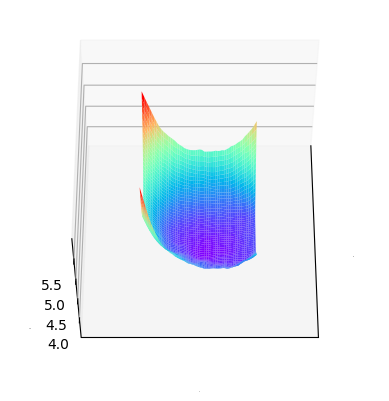
(a) TAS

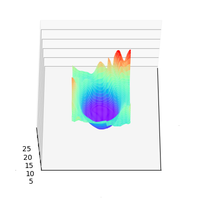
(b) SVTAS

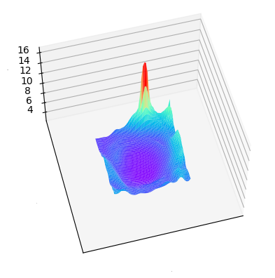
(c) SVTAS-RL(TD)

(d) SVTAS-RL(MC)

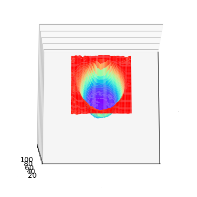
(e) F1@0.50 Error

Figure 8: Visualize optimization objective and optimization direction by 3D Surface. (a)-(d) are optimization direction surface. (e) is optimization objective error surface.

A.3 What HBRT memories?

Fig.9 shows the heat map visualization of the hierarchical memory information $m_{j}$ transmitted by HBRT. The horizontal direction is the extension direction of the streaming video, and the vertical direction is the expansion direction of the hierarchical passing. We can observe that: (a) There is obvious segment information compression in the horizontal direction. For example, the memory information of Layer 1 gradually compresses in the opposite direction of the extension of the streaming video as $j$ increases. This indicates that the memory mechanism is indeed working and it is the key to improving the Edit score. (b) In the vertical direction, as the dilation increases and the hierarchical information is transmitted, the memory information $m_{j}$ becomes richer and richer. This can provide more abundant information for the aggregation of current action segments, thereby improving the action segment integrity of full video, which is F1 score.

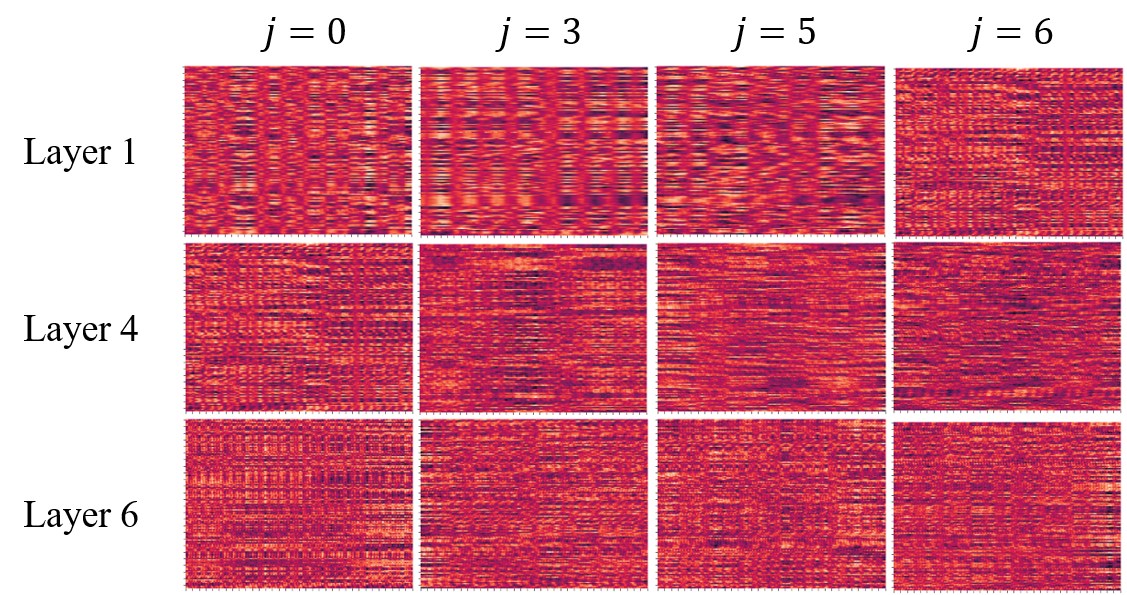
Figure 9: State Visualization in 50Salads rgb-06-1.

A.4 More Video Encoder Experiment

A.4.1 More Video Encoder Comparison

In Tab.10, as an important supplementary task for TAS, direct transferring TAS model to STAS cannot solve it, and the models of other tasks cannot perform well. This indicates that a unique model design is indeed needed for SVTAS. Among the models shown in Tab.10, the image classification (IC) models completely lose the temporal information in the feature information. Although the Action Recognition (AR) models can use the temporal information in the video clip, they cannot detect the action boundary points, which makes the Acc score of AR slightly higher than IC, but the F1 scores is very low. Video Prediction (VP) models use historical information to predict future frames, and the loss of original feature information results in very poor experimental results. Although Online Action Detection (OAD) models can use the original feature information of the current frame while seeing historical feature information, it cannot modify the action segment integrity of full video, which makes it have a huge improvement over VP in terms of Acc, but it F1 scores is still very low. The TAS model that takes the feature information of the full video sequence as input can achieve good results in experiments. However, if its input is changed to a streaming form, experiment show that model performance significantly decrease due to inconsistent optimization directions and objective. Our SVTAS-RL can effectively remember historical feature information, and estimate the gradient of the optimization objective through reinforcement learning (RL) training methods, thereby achieving extremely high single-frame accuracy and action segment integrity.

Publish	Model	Task	Acc	Edit	F1@{0.1,0.25,0.5}
CVPR 2016	ResNet [15]	IC	38.7	25.8	25.8	20.8	16.9
CVPR 2018	MobileNetV2 [37]	IC	40.9	32.2	30.5	23.6	14.2
ICLR 2021	ViT [10]	IC	28.7	33.6	21.9	17.3	8.3
CVPR 2022	Swinv2 [29]	IC	58.7	26.5	31.3	27.6	19.8
ICLR 2022	MobileViT [32]	IC	25.7	27.3	17.9	12.9	10.9
CVPR 2017	I3D [6]	AR	53.1	51.8	57.5	52.7	36.2
CVPR 2018	R(2+1)D [44]	AR	24.4	36.6	30.0	24.3	13.4
ICCV 2019	TSM [28]	AR	61.0	66.1	40.1	35.4	25.3
ICML 2021	TimeSformer [4]	AR	36.4	31.7	29.3	24.3	18.6
CVPR 2022	Swin3D [30]	AR	63.4	60.2	65.1	60.6	48.2
ICCV 2021	OadTR [47]	OAD	59.1	16.4	21.6	17.8	12.1
PAMI 2022	PredRNNV2 [48]	VP	22.7	27.9	18.8	17.7	13.5
BMVC 2021	ASformer(full) [52]	TAS	75.9	84.3	86.2	83.4	75.6
BMVC 2021	ASformer(streaming) [52]	SVTAS	70.7	68.7	76.9	70.7	57.1
ours	SVTAS-RL(MC)	SVTAS	79.9	85.6	88.0	86.5	79.3

Table 10: Video encoder comparison experiment in the split1 of GTEA.

A.4.2 More Visualization of Migration from TAS to SVTAS

Fig.10 and Fig.11 show more visual comparisons between TAS and SVTAS. The TAS task is a TAS system based on sequence-to-sequence transformation [8]. However, the SVTAS task is more inclined to action segment clustering.

(a) RGB

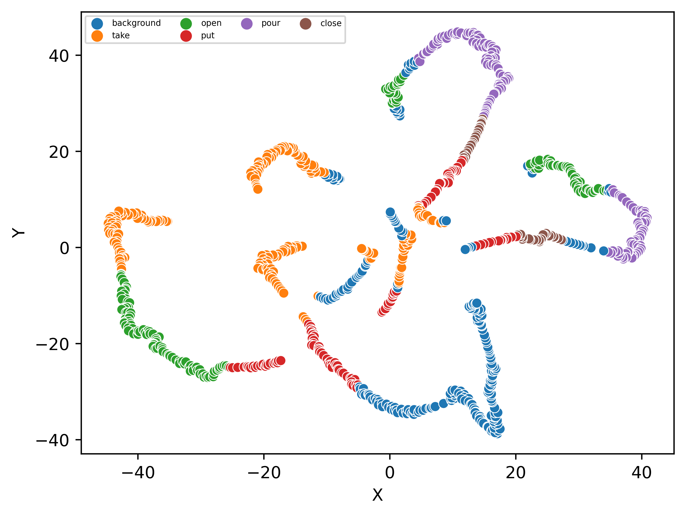
(b) TAS Input

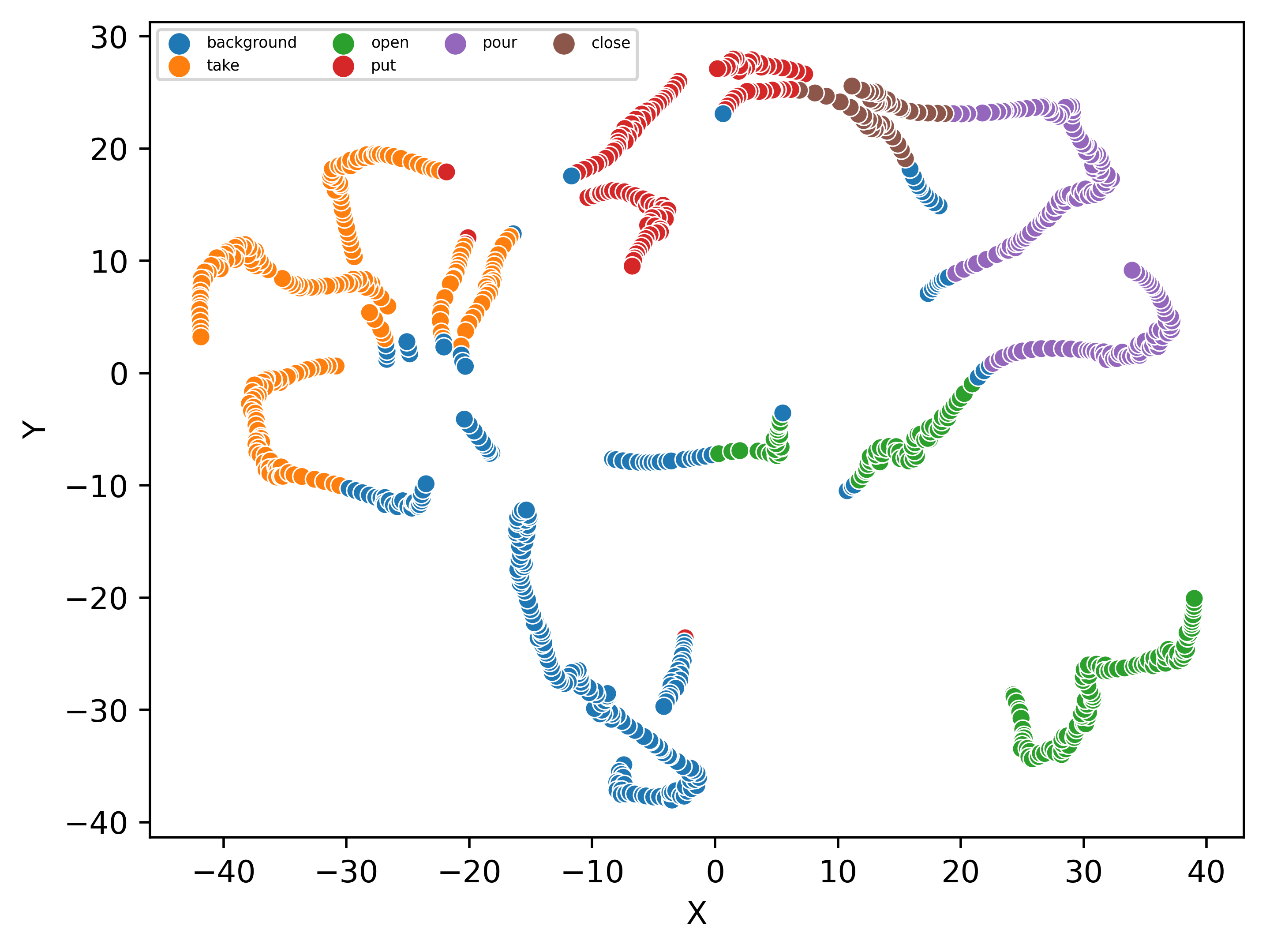
(c) TAS output

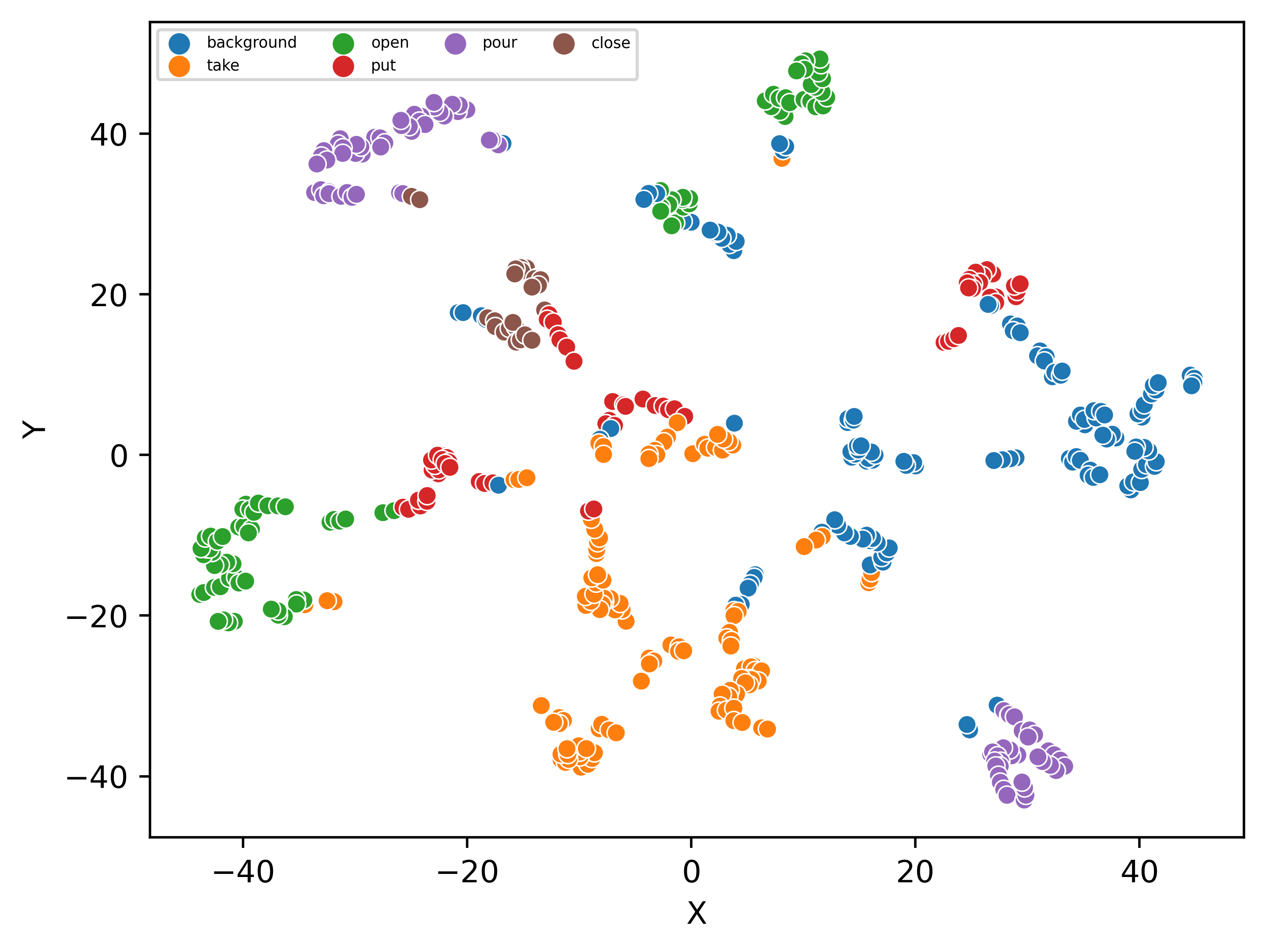
(d) SVTAS Input

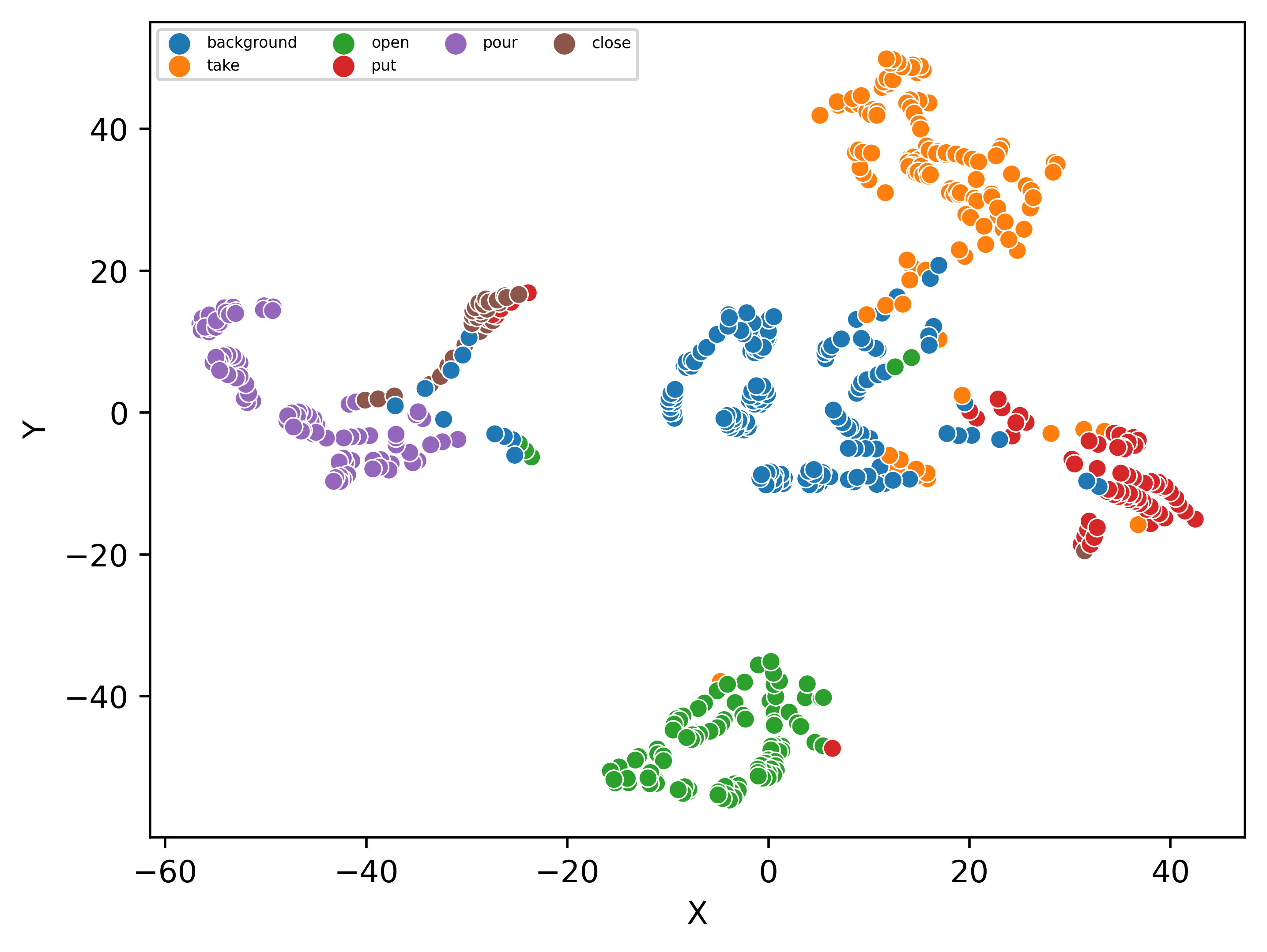
(e) SVTAS Output

Figure 10: Compare Feature. All features are extracted from GTEA S1_Cheese_C1 and visualized by t-SNE.

(a) RGB

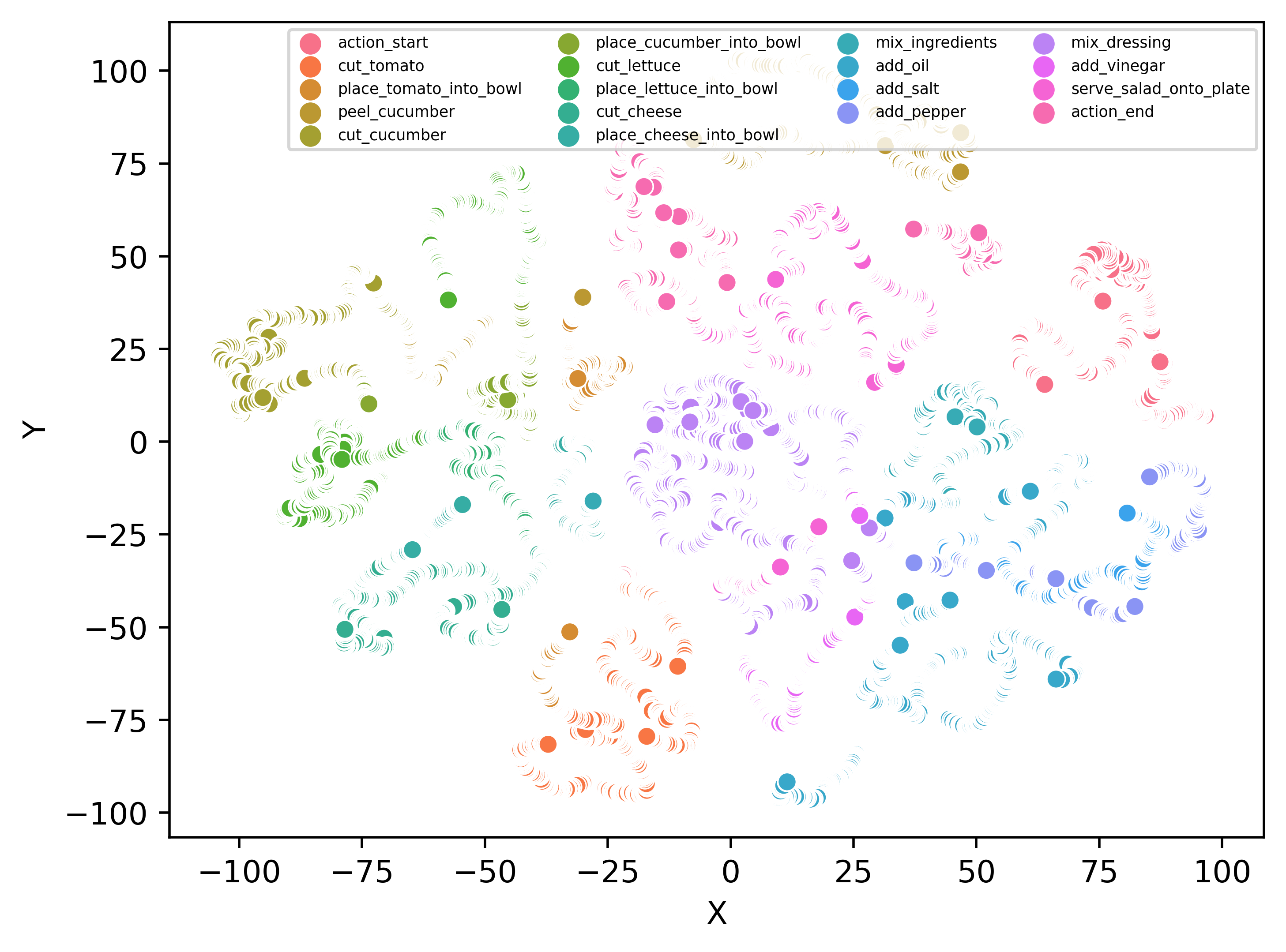
(b) TAS Input

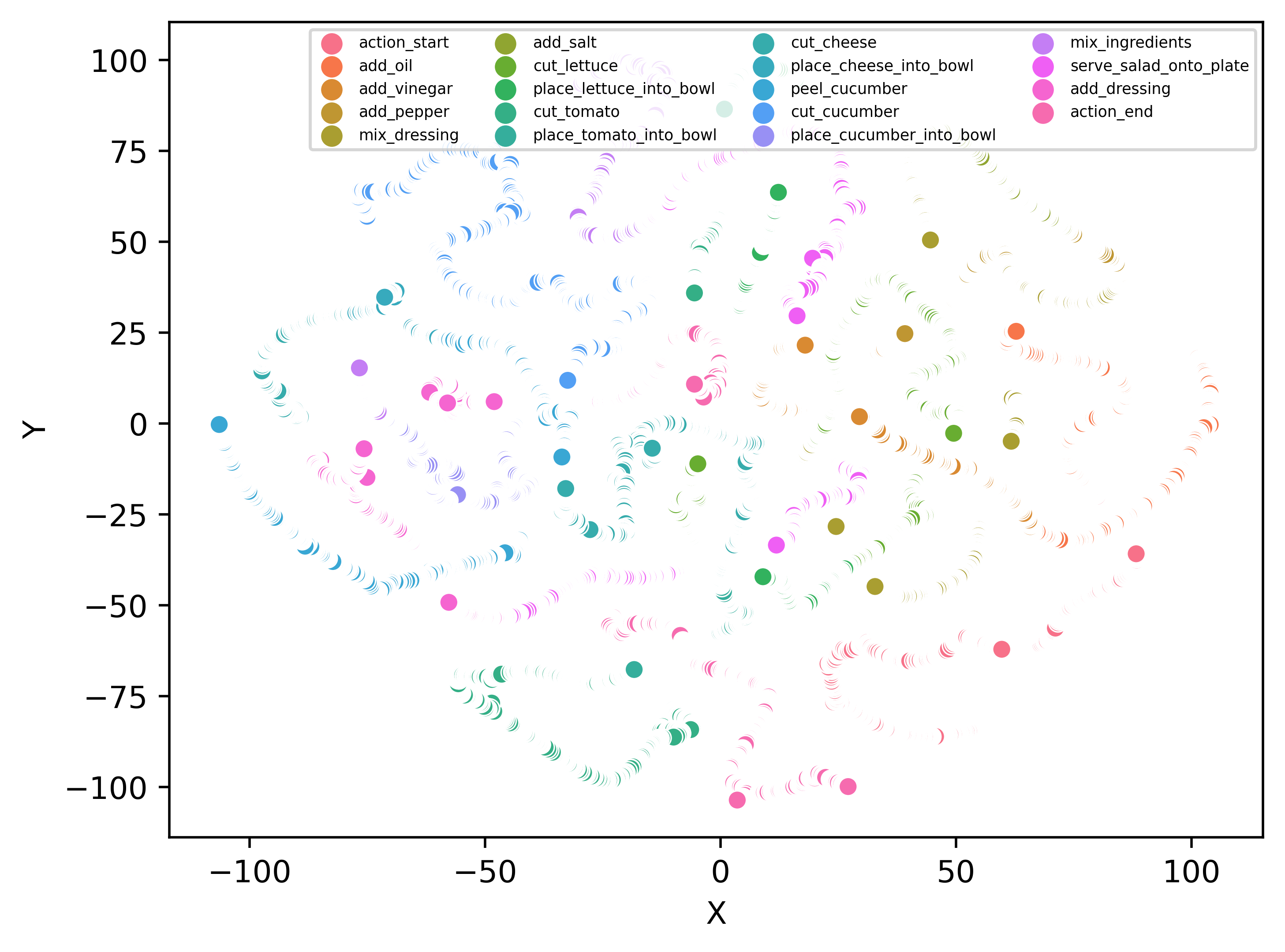
(c) TAS output

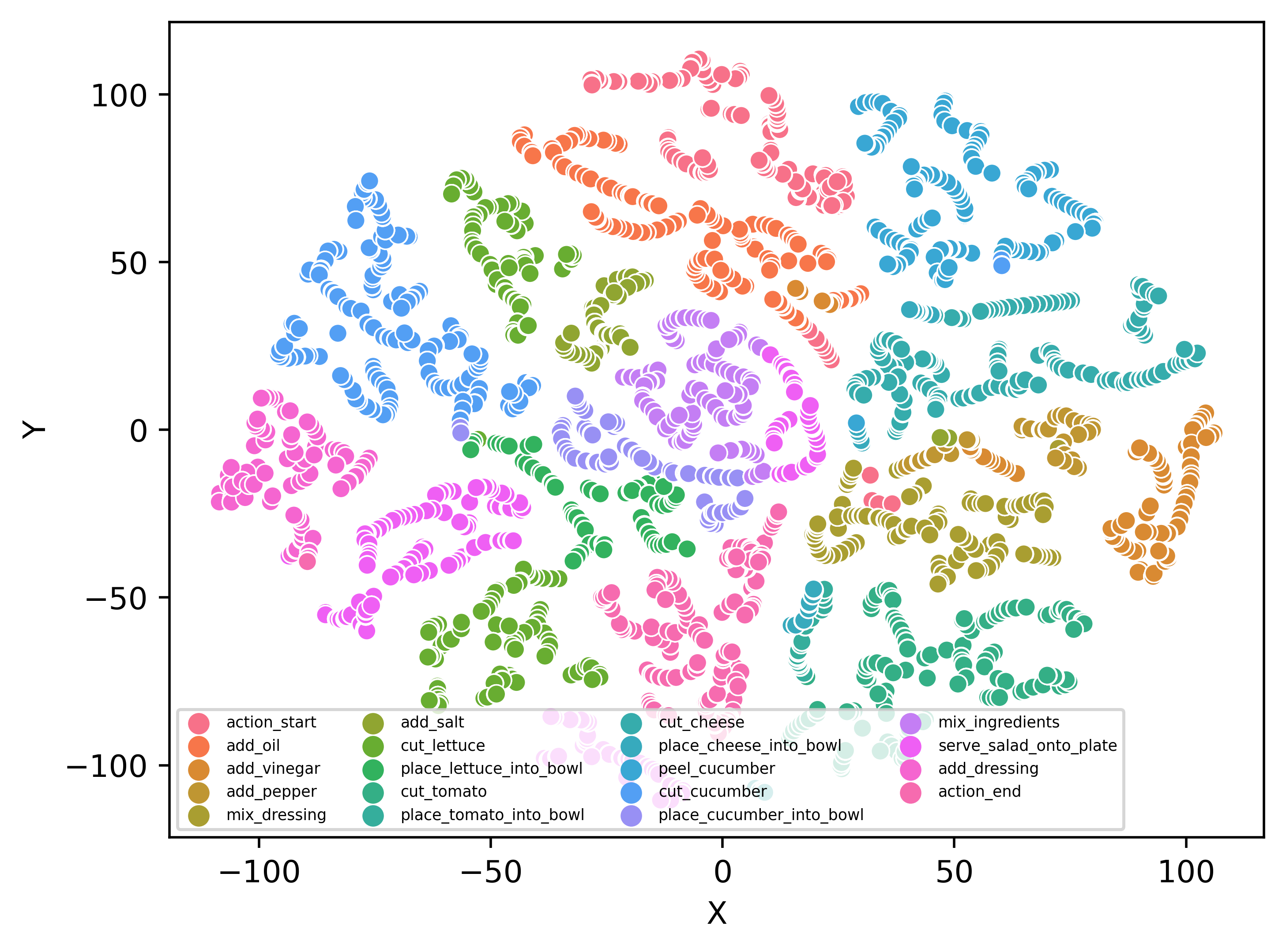
(d) SVTAS Input

(e) SVTAS Output

Figure 11: Compare Feature. All features are extracted from 50Salads rgb-10-1 and visualized by t-SNE.

A.5 Datasets Comparison

Breakfast does not perform as expected with SVTAS-RL. It is caused by the poor quality of the rgb modality for Breakfast dataset. As shown in Fig.12, we show some samples from GTEA, 50Salads and Breakfast, and compare their RGB modality and optical flow modality. We can observe that the RGB modality of GTEA and 50Saldas has clear object boundaries. However, it is difficult to distinguish object boundaries even with human eyes in RGB modality of Breakfast. In the optical flow modality, because it will be extracted through the optical flow model, even Breakfast can have good object boundaries and filter out a lot of irrelevant information, which can improve the discriminability of actions [38]. Existing TAS models are mostly multi-modality models that take both RGB modality and optical flow modality as input. This means that even if the RGB modality of samples in Breakfast is extremely poor, the required feature information can still be extracted from optical flow data (Tab.1 in the paper). However, It is an end-to-end model that our designed SVTAS-RL is, which only takes RGB data as input. This makes the model perform poorly on the Breakfast dataset. If the same RGB modality is used, our proposed model has already exceeded the performance of the full sequence (Tab.1 in the paper).

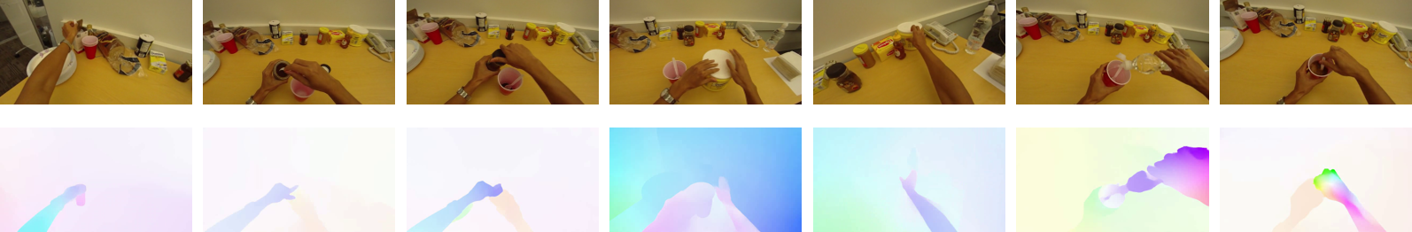
(a) GTEA S4_Coffee_C1 RGB vs Optical Flow

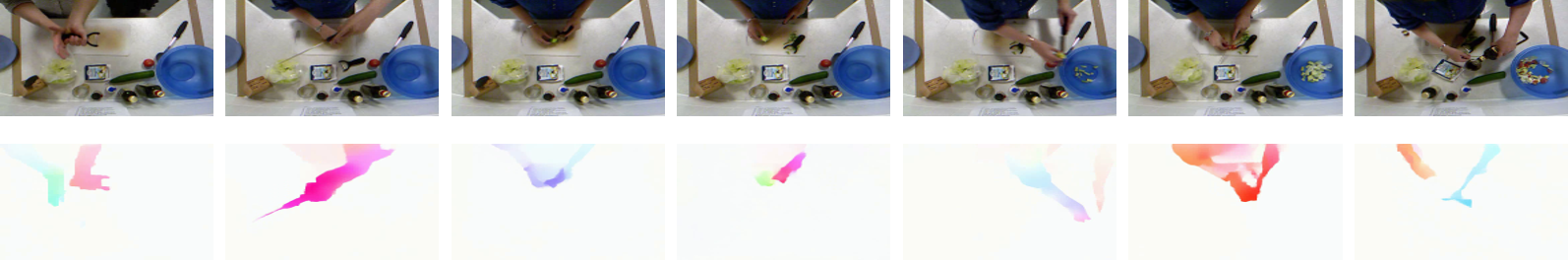
(b) 50Salads rgb-24-2 RGB vs Optical Flow

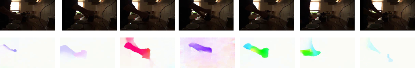
(c) Breakfast P12_cam01_P12_coffee RGB vs Optical Flow

Figure 12: RGB Modality vs Optical Flow Modality.

A.6 More Ablation Study

A.6.1 Study on Memory Length

We conducted experiments on the length of history information $m_{j}$, and the results are shown in Tab.11. SVTAS-RL achieved the best performance when the memory length is 512. As the $M$ continues to increase, SVTAS-RL continues to increase. When the memory length reaches 512, the performance is the best. When the $M$ reaches 1024, the overall performance no longer changes significantly. We speculate that this is because the time span of the dependency relationship between actions is mostly within 512.

$M$	Acc	Edit	F1@{0.1,0.25,0.5}
64	79.2	84.7	88.7	87.1	80.3
128	77.8	85.5	89.7	87.7	80.4
512	78.8	86.4	90.0	88.4	81.1
1024	79.8	85.4	89.7	88.4	81.2

Table 11: The ablation study of $M$ in 50Salads.

A.6.2 Study on pre-training parameters

For the SVTAS task, we all used pre-trained weights as the parameters of VE, which can improve the performance of the model on SVTAS. This is because the current datasets on TAS have a few samples and cannot provide sufficient training samples for VE. The ablation experiment results of pre-training parameters are shown in Tab.12. In order to verify the original effectiveness of pre-training parameters, we conducted experiments on the Swin3D model. It can be seen that the experimental results using Kinetics-600 pre-training parameters are much better than those without using pre-training. In order to verify the effectiveness of pre-training parameters on our designed SVTAS model and select more effective pre-training parameters, we conducted experiments without using pre-training parameters, using SSv2 pre-training parameters and using Kinetics-600 pre-training parameters respectively. It can be seen that the experimental results without using pre-training parameters are far inferior to those using pre-training parameters, and the experimental results using Kinetics-600 pre-training parameters are better than those using SSv2 pre-training parameters. This is because SSv2 [31] is a recognized dataset with strong temporal properties. VE with strong temporal modeling capabilities using SSv2 pre-training parameters cannot bring positive effects to SVTAS. Instead, VE trained by datasets such as Kinetics that can be recognized by image clustering can improve model performance. This proves that SVTAS is a clustering task.

Pre-trained	Model	Acc	Edit	F1@{0.1,0.25,0.5}
$\times$	Swin3D	38.9	21.4	23.7	18.4	12.6
Kinetics-600	Swin3D	84.7	59.6	69.6	67.9	61.0
$\times$	SVTAS	21.6	20.0	20.7	16.6	13.7
SSv2	SVTAS	85.1	75.1	82.7	80.5	73.9
Kinetics-600	SVTAS	86.7	78.4	85.3	83.7	77.7

Table 12: Pre-trained experiment in 50Salads.

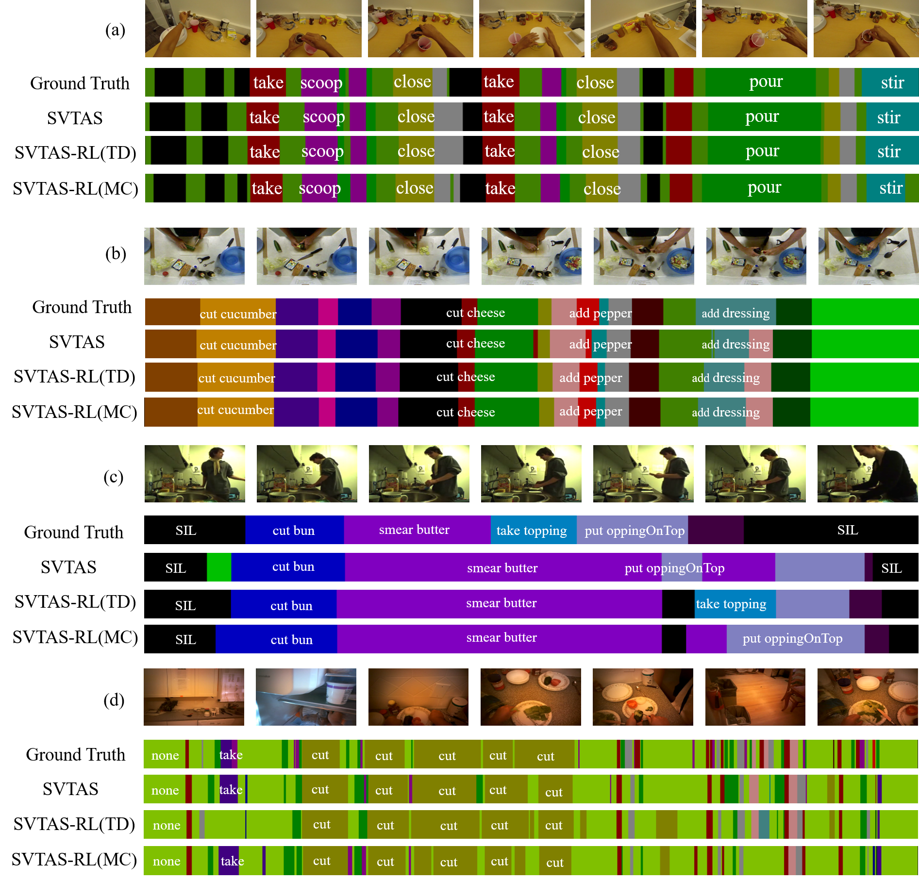
Figure 13: Quality results for datasets. (a) is from GTEA. (b) is from 50Salads. (c) is form Breakfast. (d) is from EGTEA.

A.7 Quality Results

The quality results of our designed SVTAS, SVTAS-RL(TD), and SVTAS-RL(MC) on different datasets are shown in Fig.13. It can be seen that the SVTAS model without using the RL training strategy will have errors in action category recognition when performing segmenting on streaming videos. However, SVTAS-RL(TD) and SVTAS-RL(MC) using the RL training strategy can correct this error.

References

- [1] Hyemin Ahn and Dongheui Lee. Refining action segmentation with hierarchical video representations. In Proceedings of the IEEE/CVF International Conference on Computer Vision, pages 16302–16310, 2021.
- [2] Nadine Behrmann, S Alireza Golestaneh, Zico Kolter, Jürgen Gall, and Mehdi Noroozi. Unified fully and timestamp supervised temporal action segmentation via sequence to sequence translation. In Computer Vision–ECCV 2022: 17th European Conference, Tel Aviv, Israel, October 23–27, 2022, Proceedings, Part XXXV, pages 52–68. Springer, 2022.
- [3] Richard Bellman. The theory of dynamic programming. Bulletin of the American Mathematical Society, 60(6):503–515, 1954.
- [4] Gedas Bertasius, Heng Wang, and Lorenzo Torresani. Is space-time attention all you need for video understanding? In ICML, volume 2, page 4, 2021.
- [5] Joao Carreira and Andrew Zisserman. Quo vadis, action recognition? a new model and the kinetics dataset. In proceedings of the IEEE Conference on Computer Vision and Pattern Recognition, pages 6299–6308, 2017.
- [6] Joao Carreira and Andrew Zisserman. Quo vadis, action recognition? a new model and the kinetics dataset. In proceedings of the IEEE Conference on Computer Vision and Pattern Recognition, pages 6299–6308, 2017.
- [7] Feng Cheng, Mingze Xu, Yuanjun Xiong, Hao Chen, Xinyu Li, Wei Li, and Wei Xia. Stochastic backpropagation: a memory efficient strategy for training video models. In Proceedings of the IEEE/CVF Conference on Computer Vision and Pattern Recognition, pages 8301–8310, 2022.
- [8] Guodong Ding, Fadime Sener, and Angela Yao. Temporal action segmentation: An analysis of modern technique. arXiv preprint arXiv:2210.10352, 2022.
- [9] Zhuben Dong, Yunheng Li, Yiwei Sun, Conghui Hao, Kaiyuan Liu, Tao Sun, and Shenglan Liu. Double attention network based on sparse sampling. In 2022 IEEE International Conference on Multimedia and Expo (ICME), pages 1–6. IEEE, 2022.
- [10] Alexey Dosovitskiy, Lucas Beyer, Alexander Kolesnikov, Dirk Weissenborn, Xiaohua Zhai, Thomas Unterthiner, Mostafa Dehghani, Matthias Minderer, Georg Heigold, Sylvain Gelly, et al. An image is worth 16x16 words: Transformers for image recognition at scale. arXiv preprint arXiv:2010.11929, 2020.
- [11] Yazan Abu Farha and Jurgen Gall. Ms-tcn: Multi-stage temporal convolutional network for action segmentation. In Proceedings of the IEEE/CVF conference on computer vision and pattern recognition, pages 3575–3584, 2019.
- [12] Alireza Fathi, Xiaofeng Ren, and James M Rehg. Learning to recognize objects in egocentric activities. In CVPR 2011, pages 3281–3288. IEEE, 2011.
- [13] Shang-Hua Gao, Qi Han, Zhong-Yu Li, Pai Peng, Liang Wang, and Ming-Ming Cheng. Global2local: Efficient structure search for video action segmentation. In Proceedings of the IEEE/CVF Conference on Computer Vision and Pattern Recognition, pages 16805–16814, 2021.
- [14] Alex Graves and Navdeep Jaitly. Towards end-to-end speech recognition with recurrent neural networks. In International conference on machine learning, pages 1764–1772. PMLR, 2014.
- [15] Kaiming He, Xiangyu Zhang, Shaoqing Ren, and Jian Sun. Deep residual learning for image recognition. In Proceedings of the IEEE conference on computer vision and pattern recognition, pages 770–778, 2016.
- [16] Yifei Huang, Yusuke Sugano, and Yoichi Sato. Improving action segmentation via graph-based temporal reasoning. In Proceedings of the IEEE/CVF conference on computer vision and pattern recognition, pages 14024–14034, 2020.
- [17] DeLesley Hutchins, Imanol Schlag, Yuhuai Wu, Ethan Dyer, and Behnam Neyshabur. Block-recurrent transformers. In S. Koyejo, S. Mohamed, A. Agarwal, D. Belgrave, K. Cho, and A. Oh, editors, Advances in Neural Information Processing Systems, volume 35, pages 33248–33261. Curran Associates, Inc., 2022.
- [18] Yuchi Ishikawa, Seito Kasai, Yoshimitsu Aoki, and Hirokatsu Kataoka. Alleviating over-segmentation errors by detecting action boundaries. In Proceedings of the IEEE/CVF Winter Conference on Applications of Computer Vision, pages 2322–2331, 2021.
- [19] Min-Seok Kang, Rae-Hong Park, and Hyung-Min Park. Efficient two-stream network for online video action segmentation. IEEE Access, 10:90635–90646, 2022.
- [20] Hilde Kuehne, Ali Arslan, and Thomas Serre. The language of actions: Recovering the syntax and semantics of goal-directed human activities. In Proceedings of the IEEE conference on computer vision and pattern recognition, pages 780–787, 2014.
- [21] Colin Lea, Michael D Flynn, Rene Vidal, Austin Reiter, and Gregory D Hager. Temporal convolutional networks for action segmentation and detection. In proceedings of the IEEE Conference on Computer Vision and Pattern Recognition, pages 156–165, 2017.
- [22] Colin Lea, Austin Reiter, René Vidal, and Gregory D Hager. Segmental spatiotemporal cnns for fine-grained action segmentation. In European Conference on Computer Vision, pages 36–52. Springer, 2016.
- [23] Peng Lei and Sinisa Todorovic. Temporal deformable residual networks for action segmentation in videos. In Proceedings of the IEEE Conference on Computer Vision and Pattern Recognition, pages 6742–6751, 2018.
- [24] Muheng Li, Lei Chen, Yueqi Duan, Zhilan Hu, Jianjiang Feng, Jie Zhou, and Jiwen Lu. Bridge-prompt: Towards ordinal action understanding in instructional videos. In Proceedings of the IEEE/CVF Conference on Computer Vision and Pattern Recognition, pages 19880–19889, 2022.
- [25] Shi-Jie Li, Yazan AbuFarha, Yun Liu, Ming-Ming Cheng, and Juergen Gall. Ms-tcn++: Multi-stage temporal convolutional network for action segmentation. IEEE Transactions on Pattern Analysis and Machine Intelligence, 2020.
- [26] Yin Li, Miao Liu, and James M Rehg. In the eye of beholder: Joint learning of gaze and actions in first person video. In Proceedings of the European conference on computer vision (ECCV), pages 619–635, 2018.
- [27] Yunheng Li, Zhuben Dong, Kaiyuan Liu, Lin Feng, Lianyu Hu, Jie Zhu, Li Xu, Shenglan Liu, et al. Efficient two-step networks for temporal action segmentation. Neurocomputing, 454:373–381, 2021.
- [28] Ji Lin, Chuang Gan, and Song Han. Tsm: Temporal shift module for efficient video understanding. In Proceedings of the IEEE/CVF International Conference on Computer Vision, pages 7083–7093, 2019.
- [29] Ze Liu, Han Hu, Yutong Lin, Zhuliang Yao, Zhenda Xie, Yixuan Wei, Jia Ning, Yue Cao, Zheng Zhang, Li Dong, et al. Swin transformer v2: Scaling up capacity and resolution. In Proceedings of the IEEE/CVF conference on computer vision and pattern recognition, pages 12009–12019, 2022.
- [30] Ze Liu, Jia Ning, Yue Cao, Yixuan Wei, Zheng Zhang, Stephen Lin, and Han Hu. Video swin transformer. In 2022 IEEE/CVF Conference on Computer Vision and Pattern Recognition (CVPR), pages 3192–3201, 2022.
- [31] Joanna Materzynska, Tete Xiao, Roei Herzig, Huijuan Xu, Xiaolong Wang, and Trevor Darrell. Something-else: Compositional action recognition with spatial-temporal interaction networks. In Proceedings of the IEEE/CVF Conference on Computer Vision and Pattern Recognition, pages 1049–1059, 2020.
- [32] Sachin Mehta and Mohammad Rastegari. Mobilevit: light-weight, general-purpose, and mobile-friendly vision transformer. arXiv preprint arXiv:2110.02178, 2021.
- [33] Fausto Milletari, Nassir Navab, and Seyed-Ahmad Ahmadi. V-net: Fully convolutional neural networks for volumetric medical image segmentation. In 2016 fourth international conference on 3D vision (3DV), pages 565–571. Ieee, 2016.
- [34] V. Mnih, K. Kavukcuoglu, D. Silver, A. Graves, I. Antonoglou, D. Wierstra, and M. Riedmiller. Playing atari with deep reinforcement learning. Computer Science, 2013.
- [35] André Susano Pinto, Alexander Kolesnikov, Yuge Shi, Lucas Beyer, and Xiaohua Zhai. Tuning computer vision models with task rewards. arXiv preprint arXiv:2302.08242, 2023.
- [36] Alexander Richard and Juergen Gall. Temporal action detection using a statistical language model. In Proceedings of the IEEE Conference on Computer Vision and Pattern Recognition, pages 3131–3140, 2016.
- [37] Mark Sandler, Andrew Howard, Menglong Zhu, Andrey Zhmoginov, and Liang-Chieh Chen. Mobilenetv2: Inverted residuals and linear bottlenecks. In Proceedings of the IEEE conference on computer vision and pattern recognition, pages 4510–4520, 2018.
- [38] Laura Sevilla-Lara, Yiyi Liao, Fatma Güney, Varun Jampani, Andreas Geiger, and Michael J Black. On the integration of optical flow and action recognition. In Pattern Recognition: 40th German Conference, GCPR 2018, Stuttgart, Germany, October 9-12, 2018, Proceedings 40, pages 281–297. Springer, 2019.
- [39] Bharat Singh, Tim K Marks, Michael Jones, Oncel Tuzel, and Ming Shao. A multi-stream bi-directional recurrent neural network for fine-grained action detection. In Proceedings of the IEEE conference on computer vision and pattern recognition, pages 1961–1970, 2016.
- [40] Dipika Singhania, Rahul Rahaman, and Angela Yao. Coarse to fine multi-resolution temporal convolutional network. arXiv preprint arXiv:2105.10859, 2021.
- [41] Sebastian Stein and Stephen J McKenna. Combining embedded accelerometers with computer vision for recognizing food preparation activities. In Proceedings of the 2013 ACM international joint conference on Pervasive and ubiquitous computing, pages 729–738, 2013.
- [42] Jianlin Su, Yu Lu, Shengfeng Pan, Ahmed Murtadha, Bo Wen, and Yunfeng Liu. Roformer: Enhanced transformer with rotary position embedding. arXiv preprint arXiv:2104.09864, 2021.
- [43] Richard S Sutton, David McAllester, Satinder Singh, and Yishay Mansour. Policy gradient methods for reinforcement learning with function approximation. Advances in neural information processing systems, 12, 1999.
- [44] Du Tran, Heng Wang, Lorenzo Torresani, Jamie Ray, Yann LeCun, and Manohar Paluri. A closer look at spatiotemporal convolutions for action recognition. In Proceedings of the IEEE conference on Computer Vision and Pattern Recognition, pages 6450–6459, 2018.
- [45] Dong Wang, Xiaodong Wang, and Shaohe Lv. An overview of end-to-end automatic speech recognition. Symmetry, 11(8):1018, 2019.
- [46] Weining Wang, Yan Huang, and Liang Wang. Language-driven temporal activity localization: A semantic matching reinforcement learning model. In Proceedings of the IEEE/CVF conference on computer vision and pattern recognition, pages 334–343, 2019.
- [47] Xiang Wang, Shiwei Zhang, Zhiwu Qing, Yuanjie Shao, Zhengrong Zuo, Changxin Gao, and Nong Sang. Oadtr: Online action detection with transformers. In Proceedings of the IEEE/CVF International Conference on Computer Vision, pages 7565–7575, 2021.
- [48] Yunbo Wang, Haixu Wu, Jianjin Zhang, Zhifeng Gao, Jianmin Wang, Philip Yu, and Mingsheng Long. Predrnn: A recurrent neural network for spatiotemporal predictive learning. IEEE Transactions on Pattern Analysis and Machine Intelligence, 2022.
- [49] Zhenzhi Wang, Ziteng Gao, Limin Wang, Zhifeng Li, and Gangshan Wu. Boundary-aware cascade networks for temporal action segmentation. In European Conference on Computer Vision, 2020.
- [50] Ronald J Williams. Simple statistical gradient-following algorithms for connectionist reinforcement learning. Reinforcement learning, pages 5–32, 1992.
- [51] Serena Yeung, Olga Russakovsky, Greg Mori, and Li Fei-Fei. End-to-end learning of action detection from frame glimpses in videos. In Proceedings of the IEEE conference on computer vision and pattern recognition, pages 2678–2687, 2016.
- [52] Fangqiu Yi, Hongyu Wen, and Tingting Jiang. Asformer: Transformer for action segmentation. The British Machine Vision Conference, 2021.
- [53] Jiahui Yu, Wei Han, Anmol Gulati, Chung-Cheng Chiu, Bo Li, Tara N Sainath, Yonghui Wu, and Ruoming Pang. Dual-mode asr: Unify and improve streaming asr with full-context modeling. In International Conference on Learning Representations, 2021.
- [54] Wei Zhang, Minghao Zhai, Zilong Huang, Chen Liu, Wei Li, and Yi Cao. Towards end-to-end speech recognition with deep multipath convolutional neural networks. In Intelligent Robotics and Applications: 12th International Conference, ICIRA 2019, Shenyang, China, August 8–11, 2019, Proceedings, Part VI 12, pages 332–341. Springer, 2019.
- [55] Yue Zhang, Jingju Liu, Shicheng Zhou, Dongdong Hou, Xiaofeng Zhong, and Canju Lu. Improved deep recurrent q-network of pomdps for automated penetration testing. Applied Sciences, 12(20):10339, 2022.
- [56] Kaiyang Zhou, Yu Qiao, and Tao Xiang. Deep reinforcement learning for unsupervised video summarization with diversity-representativeness reward. In Proceedings of the AAAI Conference on Artificial Intelligence, volume 32, 2018.