Nonlinear response functions and disorder: the case of photogalvanic effect

Abstract

We investigate the impact of impurity scattering on a generalized version of the circular photogalvanic effect (CPGE) in Weyl semimetals where the frequency detuning between the two orthogonally polarized beams is non-zero. Considering a minimal model with two Weyl nodes at different energies, we employ the self-consistent Born approximation (SCBA) to unravel the dependence of the associated complex correlation function on the strength of intra- and internode scattering, frequency detuning and energy difference between the two Weyl nodes. In the case of intranode scattering only, the optical response acquires Drude-like features, which we elucidate further by introducing an effective scattering strength. The Drude-like theory can even describe the response in presence of strong internode scattering if the latter has a fixed proportionality factor to the intranode scattering. By properly adjusting the frequency detuning, we also find the imaginary part of the response function to be reminiscent of a “quantized CPGE-like” form, although the real part of the response function is in general finite, and the total optical response oscillates with time due to the finite frequency offset. We finally conclude with an outlook on possible experimental consequences.

I Introduction

The optical response of solid-state systems has long been an attractive area of research, for example with regard to second-order photovoltaic effects [1, 2, 3]. A particularly interesting case is the circular photogalvanic effect (CPGE) which is associated with the spontaneous generation of a zero-frequency current as a result of the interference between one-photon absorption processes arising from two orthogonally polarized light beams of opposite frequency [4]. An initial modern derivation of the CPGE has been formulated within the nonlinear susceptibility framework that avoids the problematic divergence of the current by properly utilizing sum rules [5, 6]. This development was followed by the first experimental observations of the CPGE taking place in Si-metal-oxide-semiconductor transistors [7] and transition-metal dichalcogenides platforms [8]. The advent of topological materials [9, 10, 11, 12] invigorated the interest in the CPGE, especially when the latter was rederived in terms of the Berry connection using the Floquet formalism [13] and the Boltzmann equation [14] but also because the CPGE was connected to the Fermi-liquid property of ”anomalous velocity” caused by the orbital Berry phase of Bloch electrons [15], and the anomalous Hall response in three-dimensional materials characterized by non vanishing Berry curvature dipole [16].

In particular for topological Weyl semimetals, the generation rate of the CPGE current density of a photo-active untilted Weyl cone has been suggested to be quantized (but not topologically protected) in terms of fundamental constants [17], at least in the absence of interactions [18]. Other proposals have contemplated non quantized responses such as the dependence of the CPGE on the finite tilt of the Weyl cone [19] and its topological charge [20], the generation of an effective chiral magnetic effect leading to a giant current density response through spin-momentum locking at low frequencies [21], the enhancement of the CPGE in the presence of an emergent electromagnetic induction in momentum space and its dependence on nonlinear corrections to the Hamiltonian and on multiple bands [22]. Furthermore, the recent observation of CPGE in TaAs [23, 24] directed theoretical and experimental efforts towards investigating the link between the CPGE and benchmark properties of Weyl semimetals, in particular the Fermi arc surface states [25, 26], as a means to enable and control the confinement-induced CPGE via the characteristics of the boundary [27, 28].

In this paper, we analyze the fate of second-order optical response describing the CPGE when the two orthogonally polarized light beams have a finite frequency detuning. To that end, we focus on a minimal Weyl system with Weyl nodes located at different energies. The finite detuning is considered adequately smaller compared to both those frequencies. Introducing disorder in the form of elastic, point-like intra- and internode scattering, we study the impact of impurities on the generalized second-order optical response by determining the behavior of the real and imaginary parts of the corresponding correlation function (triangle diagram) as a function of intra- and internode scattering strengths, detuning frequency, and energy difference between the two Weyl nodes. In the case of intranode scattering, the optical response is reminiscent of the Drude-like behavior of the AC linear optical conducitivity in metals [29] which we further characterize by introducing a simple effective model with an effective scattering time. The applicability of this simple effective model is discussed as a function of the external frequency of the light beams, the detuning frequency and the intranode scattering strength. Upon including internode scattering, the effective model can describe the data to a limited degree, but only when inter- and intranode scattering are proportional to one another. The remainder of the paper is organized as follows. Sec. II defines the model Hamiltonian analyzed in this paper. The second-order response formalism is reviewed in Sec. III. The treatment of disorder on the level of a self-consistent Born approximation is detailed in Sec. IV. The effective Drude-like theory for intranode scattering is derived and discussed in Sec. V. Our relatively simple effective theory is benchmarked by comparing it to a fully numerical analysis in Sec. VI. The impact of internode scattering is detailled in Sec. VII. The results are finally summarized in Sec. VIII, where we also comment on experimental prospects.

II The model

We focus on the low-energy regime of a time-reversal-symmetry-broken and noncentrosymmetric Weyl semimetal with the minimal number of two Weyl pockets labelled by their chirality $\chi=\pm 1$. Both pockets are centered around an isotropic Weyl node. Such a setting can be modelled by a momentum-linearized two-band Hamiltonian $H_{\rm Weyl}=\sum_{\chi}H_{\chi}$ with

$$H_{\chi} ={\sum_{\bm{p}}}^{\prime}\Psi_{\bm{p}}^{\dagger}\,\left(\chi\,v_{F}\,\bm{\sigma}\cdot(\bm{p}-\bm{p}_{\chi})-\mu_{\chi}\right)\,\Psi_{\bm{p}}^{\phantom{\dagger}},$$ (1)

where $v_{F}$ denotes the Fermi velocity (taken to be identical at both nodes for simplicity), $\bm{\sigma}$ corresponds to the vector of Pauli matrices, $\bm{p}_{\chi}$ is the Weyl node momentum of the node with chirality $\chi$, and $\mu_{\chi}$ is the energy difference between that node and the chemical potential. We furthermore have $\Psi_{\bm{p}}^{\dagger}=(c_{\bm{p}\uparrow}^{\dagger},c_{\bm{p}\downarrow}^{\dagger})$, where $c_{\bm{p}s}^{\dagger}$ creates an electron of spin $s=\uparrow,\downarrow$ and three-dimensional momentum $\bm{p}$. The prime index in the summation indicates that the model is an effective low-energy theory and comes with momentum cutoffs $|\bm{p}-\bm{p}_{\chi}|\leq\Lambda$ that are much smaller than the separation of the nodes in momentum space.

Next, we incorporate disorder into the problem. We focus on local potential disorder represented by the impurity Hamiltonian

$$H_{\rm imp}=\int d^{3}r\,\Psi^{\dagger}(\bm{r})\,\sum^{N_{\text{imp}}}_{j=1}V(\bm{r}-\bm{R}_{j})\,\Psi(\bm{r}),$$ (2)

where $\Psi(\bm{r})$ is the real-space Fourier transform of $\Psi_{\bm{p}}$, and the impurity positions are labelled by $\bm{R}_{j}$. The impurity potential is chosen as $V(\bm{r})=V_{0}\,\mathds{1}\,\delta(\bm{r})$ and it describes point-like elastic scattering events from $N_{\text{imp}}$ randomly distributed impurities. Denoting $\langle\cdot\rangle_{\rm dis}$ the disorder average, the correlator is given by $\langle V(\bm{r})\,V(\bm{r}^{\prime})\rangle_{\rm dis}=W\,\delta(\bm{r}-\bm{r}^{\prime})$, where $W=|V_{0}|^{2}\,\rho_{\rm imp}$ and $\rho_{\rm imp}$ is the impurity density. Finally, we consider the Weyl semimetal to be subjected to an electric field that induces a non-equilibrium state. While restricting the electric field to be spatially homogeneous, we for the time being allow the field to be a superposition of contributions at different frequencies $\nu_{j}$, i.e. $\bm{E}(t)=\sum_{j}\bm{E}_{j}\,e^{-i\nu_{j}t}$ (the coefficients must of course be chosen such that the total field is real). We are interested in the quadratic response of the system to this field, i.e. in a situation where the electric field represents a small perturbation away from equilibrium, which in turn is described by the reference Hamiltonian $H_{0}=H_{\rm Weyl}+H_{\rm imp}$.

III Quadratic response and its disorder-free limit

As explained in Appendix A, the $\alpha$-component of the current density, $j_{\alpha}$, contains a part that is quadratic in the applied field $\bm{E}(t)=\sum_{j}\bm{E}_{j}\,e^{-i\nu_{j}t}$. This part can be expressed as

$$\langle j_{\alpha}(\bm{r},t)\rangle^{(\text{quad.})} =\sum_{\begin{subarray}{c}j,k\\ \beta,\gamma\end{subarray}}\frac{\mathcal{X}_{\alpha\beta\gamma}(0,0;\nu_{j},\nu_{k})}{-\,\nu_{j}\,\nu_{k}}E_{j,\beta}E_{k,\gamma}\,e^{i(\nu_{j}+\nu_{k})t},$$ (3)

where the conductivity tensor $\mathcal{X}_{\alpha\beta\gamma}(0,0;\nu_{j},\nu_{k})$ can be expressed in terms of the Matsubara-frequency three current correlation function $\tilde{\mathcal{X}}_{\alpha\beta\gamma}(\bm{q}_{1},\bm{q}_{2};i\Omega_{1},i\Omega_{2})$ as

$$\mathcal{X}_{\alpha\beta\gamma}(\bm{q}_{1},\bm{q}_{2};\omega_{1},\omega_{2})=\frac{\left.\tilde{\mathcal{X}}_{\alpha\beta\gamma}(\bm{q}_{1},\bm{q}_{2};i\Omega_{1},i\Omega_{2})\right|_{i\Omega_{j}\to\omega_{j}+i\,\eta_{j}}}{2},$$ (4)

where

$$\begin{split}&\tilde{\mathcal{X}}_{\alpha\beta\gamma}(\bm{q}_{1},\bm{q}_{2};i\Omega_{1},i\Omega_{2})=\int d^{3}r_{1}\int_{0}^{\beta}d\tau_{1}\int d^{3}r_{2}\int_{0}^{\beta}d\tau_{2}\\ &\quad\quad\quad\times e^{-i(\bm{q}_{1}\cdot\bm{r}_{1}-\Omega_{1}\tau_{1})}e^{-i(\bm{q}_{2}\cdot\bm{r}_{2}-\Omega_{2}\tau_{2})}\,\tilde{X}_{\alpha\beta\gamma}(\bm{r}_{1},\bm{r}_{2};\tau_{1},\tau_{2}),\\ \\ &\tilde{X}_{\alpha\beta\gamma}(\bm{r}_{1},\bm{r}_{2};\tau_{1},\tau_{2})=\langle T_{\tau}\tilde{j}_{\alpha}(0,0)\tilde{j}_{\beta}(-\bm{r}_{1},-\tau_{1})\tilde{j}_{\gamma}(-\bm{r}_{2},-\tau_{2})\rangle.\end{split}$$ (5)

In the above expressions, $E_{j,\beta}$ is the $\beta$-component of $\bm{E}_{j}$, $\Omega_{k}$ are (bosonic) Matsubara frequencies, and $\eta_{l}\to 0^{+}$. Tildes indicate quantities depending on imaginary time or Matsubara frequencies.

Thus far, the momentum $\bm{p}$ and the associated spinor $\Psi_{\bm{p}}$ were defined in the entire Brillouin zone. Since the applied electric field is taken to be spatially homogeneous, only the zero-momentum component of the electric current is excited. All current operators in the calculation are hence pocket-local. It is therefore convenient to introduce the pocket-specific notation $\Psi_{\chi\bm{k}}=\Psi_{\bm{p}_{\chi}+\bm{k}}$, where $\bm{k}$ is the momentum relative to the node, and similarly $c_{\chi\bm{k}s}=c_{\bm{p}_{\chi}+\bm{k}s}$. The Hamiltonian in Eq. (1) defines the zero-momentum current density in pocket $\chi$ as $\bm{j}_{\bm{q}=0}^{(\chi)}=\Psi_{\chi\bm{k}}^{\dagger}\,\bm{J}^{(\chi)}_{0}\,\Psi_{\chi\bm{k}}^{\phantom{\dagger}}$ with

$$\bm{J}^{(\chi)}_{0}=\chi\,v_{F}\,(-e)\,\bm{\sigma},$$ (6)

where $-e<0$ is the electron charge. In the disorder-free limit $V_{0}=0$, momentum-conservation ensures that the response function $\tilde{\mathcal{X}}_{\alpha\beta\gamma}$ is pocket-local. It can thus be written as the sum of contributions from both pockets, $\tilde{\mathcal{X}}_{\alpha\beta\gamma}=\tilde{\mathcal{X}}_{\alpha\beta\gamma}^{(+1)}+\tilde{\mathcal{X}}_{\alpha\beta\gamma}^{(-1)}$ with

$$\left.\tilde{\mathcal{X}}_{\alpha\beta\gamma}^{(\chi)}(0,0;i\Omega_{1},i\Omega_{2})\right|_{V_{0}=0}=\chi\frac{v_{F}^{3}(-e)^{3}}{T^{-1}V}$$

$$\times\sum_{\bm{q},\omega_{n}}\,\Big{[}\text{Tr}\left(\sigma_{\alpha}\,G_{\bm{q},\Omega_{1}+\Omega_{2}+\omega_{n}}^{(\chi,0)}\,\sigma_{\beta}\,G_{\bm{q},\Omega_{2}+\omega_{n}}^{(\chi,0)}\,\sigma_{\gamma}\,G_{\bm{q},\omega_{n}}^{(\chi,0)}\right)$$

$$+(\beta\leftrightarrow\gamma,\Omega_{1}\leftrightarrow\Omega_{2})\Big{]},$$ (7)

where $T$ is the temperature, $V$ the system volume, and the last term in the rectangular bracket has the same form as the first one with the indices swapped as indicated. The bare Green’s functions, finally, can be written as

$$G_{\bm{q},\omega_{n}}^{(\chi,0)}=\sum_{b=\pm 1}\frac{\frac{1}{2}\left(\mathds{1}+b\,\bm{\sigma}\cdot\bm{q}\right)}{i\omega_{n}-b\,\chi\,v_{F}\,q+\mu_{\chi}}.$$ (8)

The most convenient way to represent the physical content of Eq. (7) is via the triangle diagrams shown in Fig. 1.

(a)     (b)

Figure 1: Topologically distinct diagrams contributing to the correlation function $\tilde{\mathcal{X}}_{\alpha\beta\gamma}^{(\chi)}(0,0;i\Omega_{1},i\Omega_{2})$ presented in Eq. (7).

Since the three current correlation function $\tilde{\mathcal{X}}_{\alpha\beta\gamma}^{(\chi)}(0,0;i\Omega_{1},i\Omega_{2})$ describes the generation of a photocurrent (vertex $\alpha$) in the Weyl semimetal after a two photon absorption process (vertices $\beta$ and $\gamma$), these two triangle diagrams correspond to the two distinct relative orderings of the one photon absorption events.

IV Self-consistent Born approximation

We treat disorder on the level of the self-consistent Born approximation (SCBA). Diagrammatically, this approximation represents the resummation of diagrams of the type shown in Fig. 2.

(a)     (b)

Figure 2: 1-PI diagrams of order $|V_{0}|^{2}$ representing (a) self-energy correction, and (b) vertex correction.

We have neglected the renormalization due to tadpole diagrams, since their contribution can always be absorbed into the definition of $\mu_{\chi}$. The impact of SCBA on the quadratic response has been determined via impurity self-average. Furthermore, we generalize the quadratic response function given in Eq. (7) to an expression featuring dressed Green’s functions and vertices in the presence of the diagrams in Fig. 2. However, we note that there are several other scattering processes which can occur in the three current correlator defined in Eq. (7), but that we neglect. Examples of such processes are shown in Fig. 3. Diagram (a) describes a triple scattering event of a fermion from a single impurity, therefore the corresponding self-energy term is of the order $|V_{0}|^{3}$ and lies beyond that of the considered order $(|V_{0}|^{2})$. Diagram (b) is a two-fermion scattering event from two impurity centres and it is associated with a self-energy “crossing” term that has a significantly smaller available phase space for the scattering vectors compared to the self-energy correction in Fig. 2, and we therefore neglected such diagrams. Diagram (c) describes three-fermion scattering from a single impurity, whereas diagram (d) is a two-fermion scattering event, where one of the fermions has its energy difference from the chemical potential renormalized. In both those diagrams, the corrections cannot be classified as either purely self-energy or purely vertex ones, and we neglect them in our resummation scheme.

(a)     (b) (c)     (d)

Figure 3: Examples of scattering events which cannot be captured by dressing the correlator Eq. (7) with the self-energy term and vertex correction of Fig. 2.

The Hamiltonian in Eq. (2) induces both intra- and internode scattering of equal amplitudes. This model can be generalized by replacing the scattering amplitude $V_{0}$ by a value $V_{\rm intra}$ for states within the same pocket, and $\widetilde{W}_{\text{inter}}$ for scattering between states in different pockets. To the level of the SCBA, the corresponding self-energies and vertex corrections are generalizations of the ones derived in Ref. [31]. The Green’s function of the node with chirality $\chi$ acquires a self-energy $\Sigma$,

$$G_{\bm{q},\omega_{n}}^{(\chi,\text{SCBA})}=\sum_{b=\pm 1}\frac{\frac{1}{2}\left(\mathds{1}+b\,\bm{\sigma}\cdot\bm{q}\right)}{i\omega_{n}-b\,\chi\,v_{F}\,q+\mu_{\chi}-\Sigma^{(\chi)}_{\text{SCBA}}(i\omega_{n})},$$ (9)

which is the self-consistent solution of

$$\begin{split}&\Sigma^{(\chi)}_{\text{SCBA}}(i\omega_{n})=\\ &\widetilde{W}_{\text{intra}}\,\left(i\omega_{n}+\mu_{\chi}-\Sigma^{(\chi)}_{\text{SCBA}}(i\omega_{n})\right)\\ &\quad\quad\times\Bigg{[}-1+\frac{i\omega_{n}+\mu_{\chi}-\Sigma^{(\chi)}_{\text{SCBA}}(i\omega_{n})}{2v_{F}\Lambda}\\ &\quad\quad\quad\quad\times\ln\left(\frac{i\omega_{n}+\mu_{\chi}-\Sigma^{(\chi)}_{\text{SCBA}}(i\omega_{n})+v_{F}\Lambda}{i\omega_{n}+\mu_{\chi}-\Sigma^{(\chi)}_{\text{SCBA}}(i\omega_{n})-v_{F}\Lambda}\right)\Bigg{]}\end{split}$$

$$\begin{split}&+\widetilde{W}_{\text{inter}}\,\left(i\omega_{n}+\mu_{\bar{\chi}}-\Sigma^{(\chi)}_{\text{SCBA}}(i\omega_{n})\right)\\ &\quad\quad\quad\times\Bigg{[}-1+\frac{i\omega_{n}+\mu_{\bar{\chi}}-\Sigma^{(\chi)}_{\text{SCBA}}(i\omega_{n})}{2v_{F}\Lambda}\\ &\quad\quad\quad\quad\quad\times\ln\left(\frac{i\omega_{n}+\mu_{\bar{\chi}}-\Sigma^{(\chi)}_{\text{SCBA}}(i\omega_{n})+v_{F}\Lambda}{i\omega_{n}+\mu_{\bar{\chi}}-\Sigma^{(\chi)}_{\text{SCBA}}(i\omega_{n})-v_{F}\Lambda}\right)\Bigg{]},\end{split}$$ (10)

where the dimensionless intranode (internode) scattering strength $\widetilde{W}_{\text{intra}\,(\text{inter})}=W_{\text{intra}\,(\text{inter})}\,\Lambda/(2\pi^{2}v_{F}^{2})$ was introduced, and $\mu_{\bar{\chi}}$ denotes the energy difference of the other node from the chemical potential (i.e. $\bar{\chi}=-\chi$). The current vertex connecting a Green’s function at frequency $\omega_{n}$ to a Green’s function at $\omega_{n}+\Omega_{n}$ reads

$$\bm{J}^{(\chi)}_{\text{SCBA}}(i\omega_{n},i\Omega_{n})=\frac{\chi\,v_{F}\,(-e)}{1-Y^{(\chi)}_{\text{SCBA}}(i\omega_{n},i\Omega_{n})}\bm{\sigma},$$ (11)

with the vertex correction given as

$$\begin{split}&Y^{(\chi)}_{\text{SCBA}}(i\omega_{n},i\Omega_{n})=\dfrac{1}{6\pi^{2}(\chi v_{F})^{3}}\\ &\times\Bigg{[}-2\Lambda+\text{ln}\Bigg{[}\dfrac{i\omega_{n}-\Sigma^{(\chi)}_{\text{SCBA}}(i\omega_{n})+\Lambda}{i\omega_{n}-\Sigma^{(\chi)}_{\text{SCBA}}(i\omega_{n})-\Lambda}\Bigg{]}\Bigg{(}i\omega_{n}-\Sigma^{(\chi)}_{\text{SCBA}}(i\omega_{n})\Bigg{)}^{2}\\ &\times\Bigg{(}-\dfrac{1}{i\omega_{n}-\Sigma^{(\chi)}_{\text{SCBA}}(i\omega_{n})-i\Omega_{n}+\Sigma^{(\chi)}_{\text{SCBA}}(i\Omega_{n})}\\ &-\dfrac{2}{i\omega_{n}+i\Omega_{n}-\Sigma^{(\chi)}_{\text{SCBA}}(i\omega_{n})-\Sigma^{(\chi)}_{\text{SCBA}}(i\Omega_{n})}\Bigg{)}+\Big{(}\omega_{n}\leftrightarrow\Omega_{n}\Big{)}\,\Bigg{]}.\end{split}$$ (12)

As long as $|\omega+i\eta-\text{Re}\Sigma^{(\chi)}_{\text{SCBA}}(\omega+i\eta)|\ll\Lambda$ and $|\text{Im}\Sigma^{(\chi)}_{\text{SCBA}}(\omega+i\eta|\ll\Lambda$, which is the regime for the fermionic frequency $\omega$ considered in the remainder, the retarded versions of Green’s function $G^{(\chi,\text{SCBA})}$ and vertex correction $Y^{(\chi)}_{\text{SCBA}}$ can be simplified using the approximate self-energy solution of the self-consistent equation  (10)

$$\begin{split}&\Sigma^{(\chi)}_{\text{SCBA, approx}}(\omega+i0^{+})=\omega+\dfrac{\mu_{\chi}\widetilde{W}_{\text{intra}}+\mu_{\bar{\chi}}\widetilde{W}_{\text{inter}}}{\widetilde{W}_{\text{intra}}+\widetilde{W}_{\text{inter}}}\\ &\quad\quad+iv_{F}\Lambda\dfrac{1-\widetilde{W}_{\text{intra}}-\widetilde{W}_{\text{inter}}}{\pi(\widetilde{W}_{\text{intra}}+\widetilde{W}_{\text{inter}})}-i\dfrac{v_{F}\Lambda}{\pi(\widetilde{W}_{\text{intra}}+\widetilde{W}_{\text{inter}})}\\ &\times\Bigg{[}(1-\widetilde{W}_{\text{inter}}-\widetilde{W}_{\text{intra}})^{2}+\dfrac{\widetilde{W}_{\text{intra}}\widetilde{W}_{\text{inter}}\pi^{2}(\mu_{\chi}-\mu_{\bar{\chi}})^{2}}{(v_{F}\Lambda)^{2}}\\ &\quad\quad-i\dfrac{2\pi\Lambda(\mu_{\chi}\widetilde{W}_{\text{intra}}-\mu_{\bar{\chi}}\widetilde{W}_{\text{inter}}+\omega(\widetilde{W}_{\text{intra}}+\widetilde{W}_{\text{inter}}))}{(v_{F}\Lambda)^{2}}\Bigg{]}^{1/2}.\end{split}$$ (13)

In the relevant regime of $\omega$ defined just above, the behavior of Eqs. (10) and (13) is controlled by the parameter $(1-\widetilde{W}_{\text{inter}}-\widetilde{W}_{\text{intra}})^{2}v_{F}\Lambda/|\omega|$ [31]. In the absence of internode scattering $(\widetilde{W}_{\text{inter}}=0)$, we find $\text{Re}\Sigma/|\omega|\to-\infty$ as $\omega\to 0$ when $\widetilde{W}_{\text{intra}}=1$. Therefore, $\widetilde{W}_{\text{intra,crit}}=1$ is termed the critical scattering strength, and it is the upper threshold for the interval of $\widetilde{W}_{\text{intra}}$-values we consider in the remainder. With these definitions, we can express the quadratic response function in the self-consistent Born approximation as

$$\begin{split}&\left.\tilde{\mathcal{X}}_{\alpha\beta\gamma}^{(\chi,\text{SCBA})}(0,0;i\Omega_{1},i\Omega_{2})\right|_{\widetilde{W}_{\text{inter}}=0}=\frac{1}{T^{-1}V}\sum_{\bm{q},\omega_{n}}\Bigg{[}\\ &\text{Tr}\Bigg{(}G_{\bm{q},\Omega_{1}+\Omega_{2}+\omega_{n}}^{(\chi,\text{SCBA})}\,{J}^{(\chi)}_{\text{SCBA},\beta}(i\omega_{n}+\Omega_{2},i\Omega_{1})\,G_{\bm{q},\Omega_{2}+\omega_{n}}^{(\chi,\text{SCBA})}\\ &\times{J}^{(\chi)}_{\text{SCBA},\gamma}(i\omega_{n},i\Omega_{2})\,G_{\bm{q},\omega_{n}}^{(\chi,\text{SCBA})}\,{J}^{(\chi)}_{\text{SCBA},\alpha}(i\omega_{n},i\Omega_{1}+\Omega_{2})\,\Bigg{)}\\ &+(\beta\leftrightarrow\gamma,\Omega_{1}\leftrightarrow\Omega_{2})\Bigg{]}.\end{split}$$ (14)

After deforming the sum over Matsubara frequencies into integrals running along the branch cuts of the self-energies and vertices, we obtain

$$\left.\tilde{\mathcal{X}}_{\alpha\beta\gamma}^{(\chi,\text{SCBA})}(0,0;i\Omega_{1},i\Omega_{2})\right|_{\widetilde{W}_{\text{inter}}=0}=\frac{i}{3}\chi\epsilon^{\alpha\beta\gamma}(-e)^{3}v_{F}^{3}\int_{0}^{\Lambda}dk\frac{k^{2}}{2\pi^{2}}\sum_{b_{1},b_{2},b_{3}=\pm 1}\tilde{\delta}_{b_{1},b_{2},b_{3}}\,\frac{i}{2\pi}\int_{-\infty}^{\infty}d\omega\,n_{F}(\omega)$$

$$\times\Biggl{(}\Biggl{[}\frac{1}{1-Y^{(\chi)}_{\text{SCBA}}(\omega+i\eta,\omega+i\Omega_{1}+i\Omega_{2})}\,\frac{1}{1-Y^{(\chi)}_{\text{SCBA}}(\omega+i\eta+i\Omega_{2},\omega+i\eta)}\,\frac{1}{\omega+i\eta+\mu_{\chi}-b_{3}v_{F}k-\Sigma^{(\chi)}_{\text{SCBA}}(\omega+i\eta)}$$

$$\quad-\frac{1}{1-Y^{(\chi)}_{\text{SCBA}}(\omega-i\eta,\omega+i\Omega_{1}+i\Omega_{2})}\,\frac{1}{1-Y^{(\chi)}_{\text{SCBA}}(\omega-i\eta+i\Omega_{2},\omega-i\eta)}\,\frac{1}{\omega-i\eta+\mu_{\chi}-b_{3}v_{F}k-\Sigma^{(\chi)}_{\text{SCBA}}(\omega-i\eta)}\Biggr{]}$$

$$\times\frac{1}{\omega+\mu_{\chi}+\Omega_{1}+i\Omega_{2}-b_{1}v_{F}k-\Sigma^{(\chi)}_{\text{SCBA}}(\omega+i\Omega_{1}+i\Omega_{2})}\,\frac{1}{\omega+\mu_{\chi}+i\Omega_{2}-b_{2}v_{F}k-\Sigma^{(\chi)}_{\text{SCBA}}(\omega+i\Omega_{2})}$$

$$\times\frac{1}{1-Y^{(\chi)}_{\text{SCBA}}(\omega+i\Omega_{1}+i\Omega_{2},\omega+i\Omega_{2})}$$

$$+\Biggl{[}\frac{1}{1-Y^{(\chi)}_{\text{SCBA}}(\omega+i\Omega_{1},\omega+i\eta)}\,\frac{1}{1-Y^{(\chi)}_{\text{SCBA}}(\omega+i\eta,\omega-i\Omega_{2})}\,\frac{1}{\omega+i\eta+\mu_{\chi}-b_{2}v_{F}k-\Sigma^{(\chi)}_{\text{SCBA}}(\omega+i\eta)}$$

$$\quad-\frac{1}{1-Y^{(\chi)}_{\text{SCBA}}(\omega+i\Omega_{1},\omega-i\eta)}\,\frac{1}{1-Y^{(\chi)}_{\text{SCBA}}(\omega-i\eta,\omega-i\Omega_{2})}\,\frac{1}{\omega-i\eta+\mu_{\chi}-b_{2}v_{F}k-\Sigma^{(\chi)}_{\text{SCBA}}(\omega-i\eta)}\Biggr{]}$$

$$\times\frac{1}{\omega+\mu_{\chi}+i\Omega_{1}-b_{1}v_{F}k-\Sigma^{(\chi)}_{\text{SCBA}}(\omega+i\Omega_{1})}\,\frac{1}{\omega+\mu_{\chi}-i\Omega_{2}-b_{3}v_{F}k-\Sigma^{(\chi)}_{\text{SCBA}}(\omega-i\Omega_{2})}$$

$$\times\frac{1}{1-Y^{(\chi)}_{\text{SCBA}}(\omega-i\Omega_{2},\omega+i\Omega_{1})}$$

$$+\Biggl{[}\frac{1}{1-Y^{(\chi)}_{\text{SCBA}}(\omega+i\eta-i\Omega_{1}-i\Omega_{2},\omega+i\eta)}\,\frac{1}{1-Y^{(\chi)}_{\text{SCBA}}(\omega+i\eta,\omega-i\Omega_{1})}\,\frac{1}{\omega+i\eta+\mu_{\chi}-b_{1}v_{F}k-\Sigma^{(\chi)}_{\text{SCBA}}(\omega+i\eta)}$$

$$-\frac{1}{1-Y^{(\chi)}_{\text{SCBA}}(\omega-i\eta-i\Omega_{1}-i\Omega_{2},\omega-i\eta)}\,\frac{1}{1-Y^{(\chi)}_{\text{SCBA}}(\omega-i\eta,\omega-i\Omega_{1})}\,\frac{1}{\omega-i\eta+\mu_{\chi}-b_{1}v_{F}k-\Sigma^{(\chi)}_{\text{SCBA}}(\omega-i\eta)}\Biggr{]}$$

$$\times\frac{1}{\omega+\mu_{\chi}-i\Omega_{1}-b_{2}v_{F}k-\Sigma^{(\chi)}_{\text{SCBA}}(\omega-i\Omega_{1})}\,\frac{1}{\omega+\mu_{\chi}-i\Omega_{1}-i\Omega_{2}-b_{3}v_{F}k-\Sigma^{(\chi)}_{\text{SCBA}}(\omega-i\Omega_{1}-i\Omega_{2})}$$

$$\times\frac{1}{1-Y^{(\chi)}_{\text{SCBA}}(\omega-i\Omega_{1},\omega-i\Omega_{1}-i\Omega_{2})}\Biggr{)}+(\beta\leftrightarrow\gamma,\Omega_{1}\leftrightarrow\Omega_{2}),$$ (15)

where $\tilde{\delta}_{b_{1},b_{2},b_{3}}=1-\delta_{b_{1}b_{2}}\delta_{b_{1}b_{3}}$ and $n_{F}(\omega)=\big{[}1+\text{exp}(\omega/T)\big{]}^{-1}$.

V Effective Drude-like theory for intranode Scattering

We begin by discussing the case of pure intranode scattering at a Weyl node of chirality $\chi$ by setting $\widetilde{W}_{\text{inter}}=0$. To unearth the physical content of Eq. (15), it is helpful to perfom several ad-hoc approximations, on which we further comment below through the comparison to the full numerical solution. First, we neglect vertex corrections in Eq. (15) by setting $Y=0$. Second, we approximate the self-energy by a constant level broadening, $\Sigma(z)\to-i\Gamma\text{sgn}(\text{Im}(z))$, and replace $i\Omega_{j}\to\omega_{j}+i\eta_{j}$ where $\eta_{j}\to 0^{+}$. Third, we approximate the Lorentzian spectral density functions appearing in Eq. (15) by Dirac delta functions, which allows us to perform the frequency integration. As detailed in Appendix B, the remaining momentum integrals are evaluated under the approximation that $|\Gamma|\ll|\omega_{1}+\omega_{2}|$, $|\omega_{1}|$, $|\omega_{2}|$, and in the limit of zero temperature. Also, we are interested in the response to a superposition of two orthogonal, linearly polarized electric fields with frequencies $\omega_{1}=\omega_{0}$ and $\omega_{2}=-\omega_{0}+\delta\omega$,

$$\bm{E}(t)=\begin{pmatrix}E_{x}\,\cos(\omega_{1}\,t)\\ E_{y}\,\sin(\omega_{2}t)\\ 0\end{pmatrix}.$$ (16)

The part of the quadratic response oscillating at frequency $\delta\omega$ can then be written as

$$\begin{split}&j_{z,\delta\omega}^{(\chi)}(t)=-\dfrac{e^{3}\chi E_{x}E_{y}}{24\pi}\beta_{0}(\delta\omega,\Gamma,t)F(\omega_{0},\Gamma,\mu_{\chi}),\\ &\beta_{0}(\delta\omega,\Gamma,t)=\dfrac{\delta\omega}{\delta\omega^{2}+4\Gamma^{2}}\sin(\delta\omega\,t)-\dfrac{2\Gamma}{\delta\omega^{2}+4\Gamma^{2}}\cos(\delta\omega\,t),\\ &F(\omega_{0},\Gamma,\mu_{1})=\frac{1}{\pi}\,\text{Im}\left(\ln\left(4|\mu_{1}|^{2}-(\omega_{0}+i\Gamma)^{2}\right)\right).\end{split}$$ (17)

In the limit $\Gamma\to 0$, where $F(\omega_{0})\to-\text{sgn}(\omega_{0})\theta(|\omega_{0}|-2|\mu_{1}|)$, we recover the quantized CPGE response discussed in Ref. [17]. Note that the limits $\Gamma\to 0$ and $\delta\omega\to 0$ do not commute and the quantized CPGE response is obtained by performing the limit $\Gamma\to 0$ first.

For finite $\Gamma$, the quantized CPGE response is modified in two important ways. First, the onset as a function of $\omega_{0}$ is smeared out in a frequency range of order $\Gamma$ around $2|\mu_{1}|$, which is described by $F(\omega_{0},\mu_{1})$. Second, the response function acquires a Drude-like form $\sim(\delta\omega+i2\Gamma)^{-1}$. This means that the current, unlike in the clean limit, does not diverge linearly in time anymore, but acquires a finite amplitude. It is interesting to note that the expression for $j_{z,\delta\omega}^{(\chi)}(t)$ given in Eq. (17), which we recall has been derived under the assumption $|\Gamma|\ll|\delta\omega|$, smoothly connects to the results of Ref. [32] derived for finite $|\Gamma|$ but $\delta\omega=0$: there it was argued that after switching on a circularly polarized beam of light, a Weyl semimetal would first show a CPGE-current that increases linearly in time, but that this current would level off for times larger than the scattering time $t=|\Gamma|^{-1}$ and in the steady state, the current would thus be $j_{z}\sim\Gamma^{-1}$. This statement is reproduced by our quadratic response approach (see Eq. (17)) which, much like linear response theory, yields the response to an electric field that has been switched on in the infinite past, and is hence also concerned with long-time responses. The fact that our calculation predicts a current whose amplitude is in complete agreement with the findings of Ref. [32] at $\delta\omega=0$ and finite $\Gamma$ suggests that Eq. (17) can smoothly interpolate between the limiting cases $|\Gamma|\gg|\delta\omega|$ and $|\Gamma|\ll|\delta\omega|$ at least for some finite range of parameters.

However, it should be emphasized that the condition $|\delta\omega|\ll|\omega_{0}|$ must be respected to recover the quantized CPGE result of Ref. [17] in the disorder-free limit. Keeping corrections of the order $\mathcal{O}(\delta\omega^{3}/\omega^{3}_{0})$ even when $\Gamma=0$, Eq. (17) becomes

$$\begin{split}&j_{z,\delta\omega}^{(\chi)}(t)\approx\dfrac{-e^{3}\chi E_{x}E_{y}}{24\pi}\dfrac{\sin\delta\omega\,t}{\delta\omega}\Bigg{(}1-\dfrac{\delta\omega^{2}}{\omega^{2}_{0}}\Bigg{)},\\ &F(\omega_{0},\mu_{1})=-\text{sgn}(\omega_{0})\theta(|\omega_{0}|-2|\mu_{1}|).\end{split}$$ (18)

Turning away from the limit $|\delta\omega|\ll|\omega_{0}|$ will thus alter the resonance structure of Eq. (15) and will affect the functional form of the current density in Eq. (3).

VI Full numerical solution for intranode scattering

After replacing $i\Omega_{j}\to\omega_{j}+i\eta_{j}$, Eq. (15) can also be evaluated numerically. For that purpose, we use the approximate self-energy given in Eq. (13) as well as the vertex corrections Eq. (12). The corresponding numerical results are shown in Fig. 4 for the case $\omega_{0}=3$, $\delta\omega=10^{-3}$.

To compare those numerical results to the Drude-like formula in Eq. (17), we set $\Gamma=-\text{Im}\,\Sigma^{(\chi)}_{\text{SCBA, approx.}}$. The thus evaluated response corresponds to electrons being excited from an energy $-\omega_{0}/2$ below the Weyl node to an energy $+\omega_{0}/2$ above the Weyl node, and the self-energy should hence be evaluated at the corresponding frequency. This physical argument agrees with an analysis of the peak structure of the integrand in Eq. (15): neglecting vertex corrections, the terms in the square brackets correspond to density of states factors that peak at $\omega+i\eta=\pm v_{F}q+\Sigma^{(\chi)}_{\text{SCBA}}(\omega+i\eta)$ and plugging this frequency into the propagators yields peaks at $2v_{F}q=\pm\omega_{0}$. We hence evaluate the self-energy at frequency $\omega$ that solves the equation $\omega-\text{Re}\,\Sigma^{(\chi)}_{\text{SCBA, approx}}(\omega)=\omega_{0}/2$. Fig. 5 depicts the imaginary part of the self-energy thus determined as a function of $\widetilde{W}_{\text{intra}}$.

For the response function shown in Fig. 4, we find that the Drude-like approximation $\Gamma=-\text{Im}\,\Sigma^{(\chi)}_{\text{SCBA, approx.}}$ describes $\mathcal{X}_{\alpha\beta\gamma}^{(\chi,\text{SCBA})}$ qualitatively well even close to the critical scattering regime $\widetilde{W}_{\text{intra, crit}}=1$. Thus the range of applicability of our Drude-like response function is confirmed to extend beyond the limit $|\Gamma|\ll|\delta\omega|$. In the scattering regime $\widetilde{W}_{\text{intra}}\lesssim 0.6$, the features of $\mathcal{X}_{\alpha\beta\gamma}^{(\chi,\text{SCBA})}$ can also be described (in fact even slightly better) by the further approximated formulae $\text{Re}\,\Sigma^{(\chi)}_{\text{SCBA, approx}}(\omega)=-\widetilde{W}_{\text{intra}}\,\omega/(1-\widetilde{W}_{\text{intra}})$ and $\Gamma=\pi\,\widetilde{W}_{\text{intra}}\,\omega^{2}/2v_{F}\Lambda(1-\widetilde{W}_{\text{intra}})^{3}$ [31], which is also indicated in Fig. 5. This simplification predicts the peak value of $\text{Re}\,\mathcal{X}$ to occur at an estimated scattering strength

$$\widetilde{W}_{\text{intra, cross}}=\dfrac{1}{1+\dfrac{\pi\omega^{2}_{0}}{4v_{F}\delta\omega\Lambda}}$$ (19)

under the condition $\omega-\text{Re}\,\Sigma^{(\chi)}_{\text{SCBA, approx}}(\omega)=\omega_{0}/2$. The disorder scale $\widetilde{W}_{\text{intra, cross}}$ defines a crossover scale between the response regime $|\delta\omega|>2|\Gamma|$ associated with the increase-with-scattering behavior of $\text{Im}\,\Sigma^{(\chi)}_{\text{SCBA, approx}}$ connecting smoothly to the limiting case $|\delta\omega|\gg|\Gamma|$ with a current profile $j_{z,\delta\omega}^{(\chi)}(t)\sim\delta\omega^{-1}\,\sin(\delta\omega\,t)$, and the response regime $|\delta\omega|<2|\Gamma|$, where decay sets in according to $\text{Im}\,\Sigma^{(\chi)}_{\text{SCBA, approx}}$ with the corresponding limiting case $|\delta\omega|\ll|\Gamma|$ predicting the current profile $j_{z,\delta\omega}^{(\chi)}(t)\sim\Gamma^{-1}\,\cos(\delta\omega\,t)$.

A complementary viewpoint is the scenario where the ratio $|\Gamma|/|\delta\omega|$ is changed by varying the frequency detuning $\delta\omega$ for fixed scattering strength $\widetilde{W}_{\text{intra}}$. The evolution of $\mathcal{X}_{\alpha\beta\gamma}^{(\chi,\text{SCBA})}$ as a function of $\delta\omega$ is depicted in Fig. 6. We find that the regime $\delta\omega\gg\Gamma$, in which the amplitude of $\text{Im}\,\mathcal{X}$ takes the “quantized CPGE”-value, can also be reached by tuning $\delta\omega$, but only provided the condition $\delta\omega\ll\omega_{0}$ is satisfied, see Eq. (18). However, it should again be noted that as far as the total response Eq. (3) is concerned, the current density is an oscillatory function in time domain with the oscillation period determined by $\delta\omega$, unlike the disorder-free CPGE response displaying linear-with-time increase of current density [17]. Furthermore, we observe a similarly good agreement between the approximate Drude-like response and the full numerics as for varying scattering strength as above, including also the regime for $\Gamma$ far beyond the limit $|\Gamma|\ll|\delta\omega|$. Thus, the $\pi$-phase shift and distinct dependence on $\delta\omega$ in the two regimes provide clear experimental signatures of the Drude-like behavior of the quadratic response. More generally, the amplitude and phase (with respect to the driving field) of the current as a function of $|\delta\omega|/|\Gamma|$ should enable a full experimental determination of the complex-valued response function $\mathcal{X}_{\alpha\beta\gamma}$ that allows to compare with the behavior predicted by our calculation.

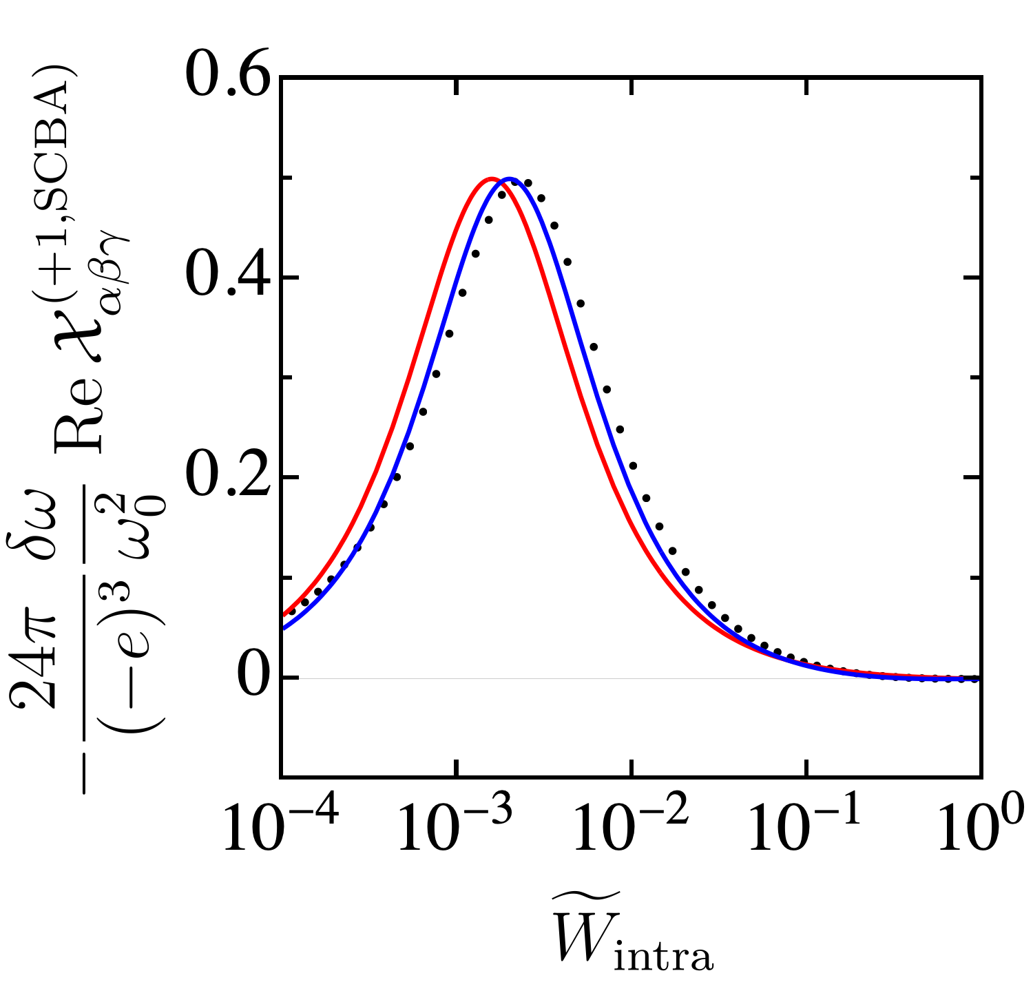
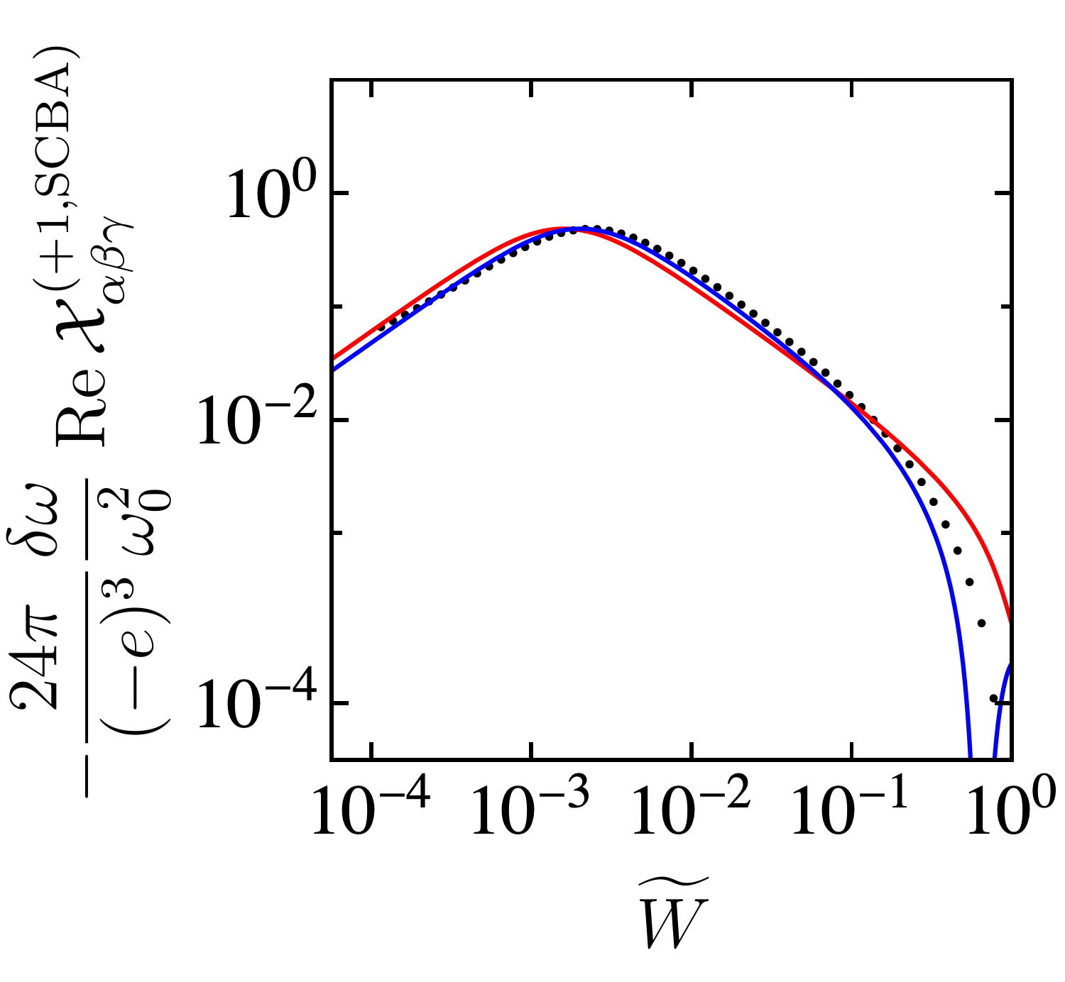
(a)     (b)
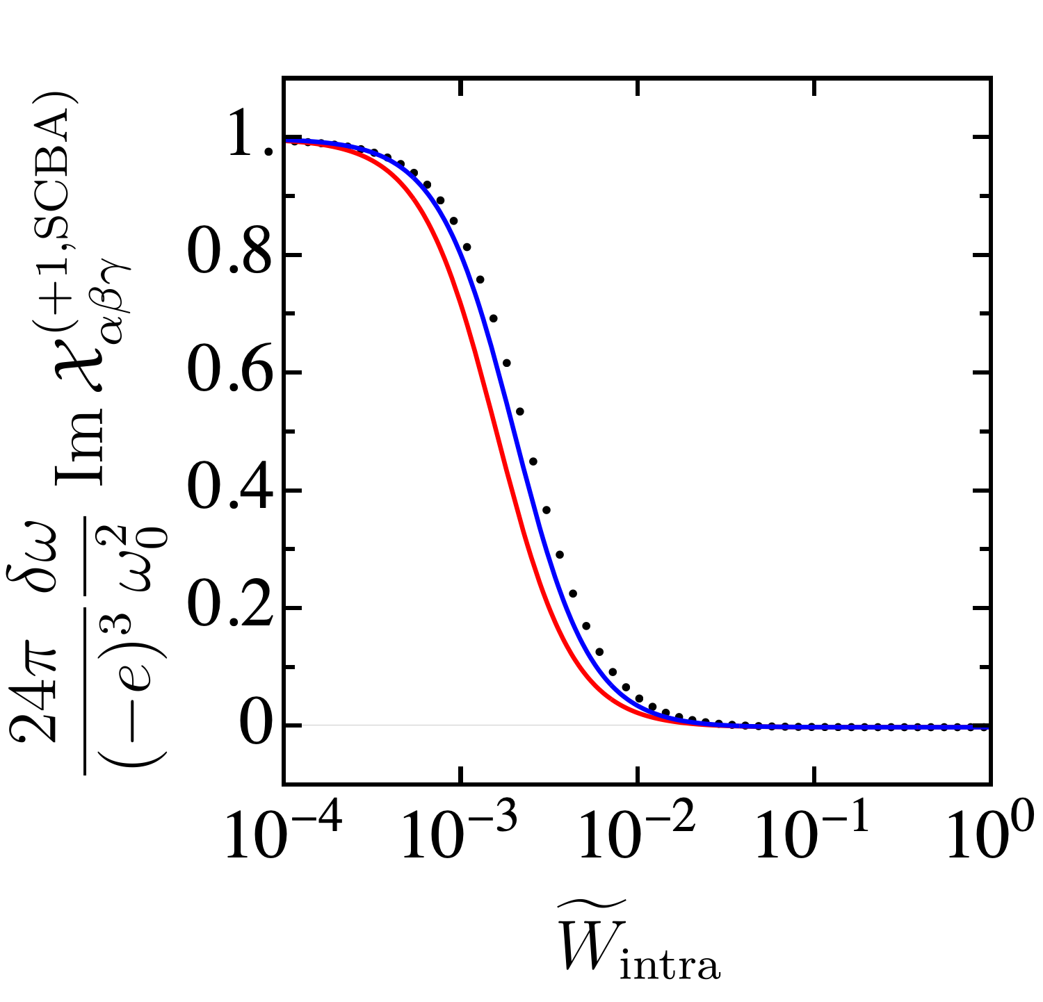
(c)     (d)

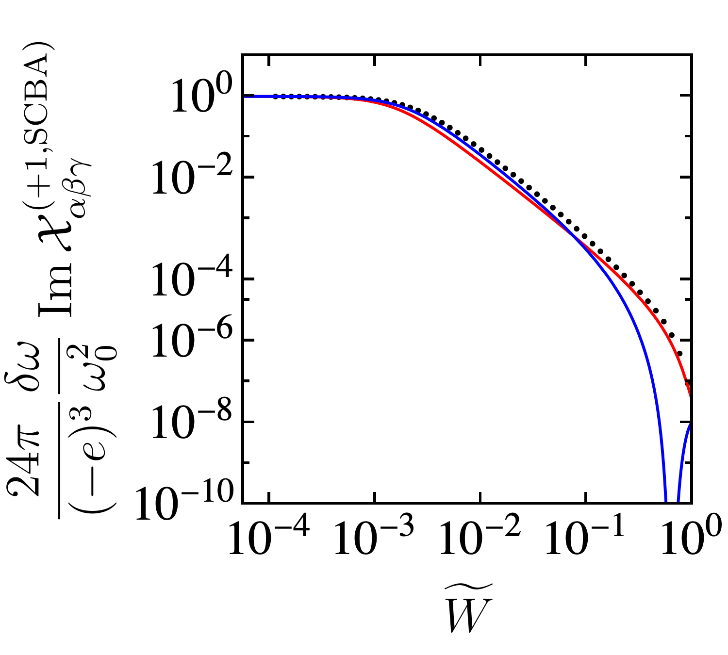
Figure 4: Panels (a) and (b) show the normalized real and imaginary parts of the response function $\mathcal{X}_{\alpha\beta\gamma}^{(+1,\text{SCBA})}\equiv\left.{\mathcal{X}}_{\alpha\beta\gamma}^{(+1,\text{SCBA})}(0,0;\omega_{0},-\omega_{0}+\delta\omega)\right|_{\widetilde{W}_{\text{inter}}=0}$ presented in Eq. (15) on linear scale as a function of the dimensionless intranode scattering strength $\widetilde{W}_{\text{intra}}$ in the absence of internode scattering. Panels (c) and (d) show the same data as (a) and (b) but on logarithmic scale. The black dots show the numerical evaluation of Eq. (15) with the replacements $i\Omega_{j}\to\omega_{j}+i\,\eta_{j}$, $\omega_{1}=\omega_{0}$, $\omega_{2}=-\omega_{0}+\delta\omega$, $\omega_{0}=3$, $\delta\omega=10^{-3}$, $\mu=1$, $v_{F}=1$, $\Lambda=25$, $\eta_{1}=1.05\cdot 10^{-5}$, $\eta_{2}=0.95\cdot 10^{-5}$, and $\eta=0.9\cdot 10^{-6}$. The red and blue lines depict the effective Drude-like expression in Eq. (17) when setting $\Gamma=-\text{Im}\,\Sigma^{(+1)}_{\text{SCBA, approx.}}$ and $\Gamma=\pi\,\widetilde{W}_{\text{intra}}\,\omega^{2}/2v_{F}\Lambda(1-\widetilde{W}_{\text{intra}})^{3}$ respectively.

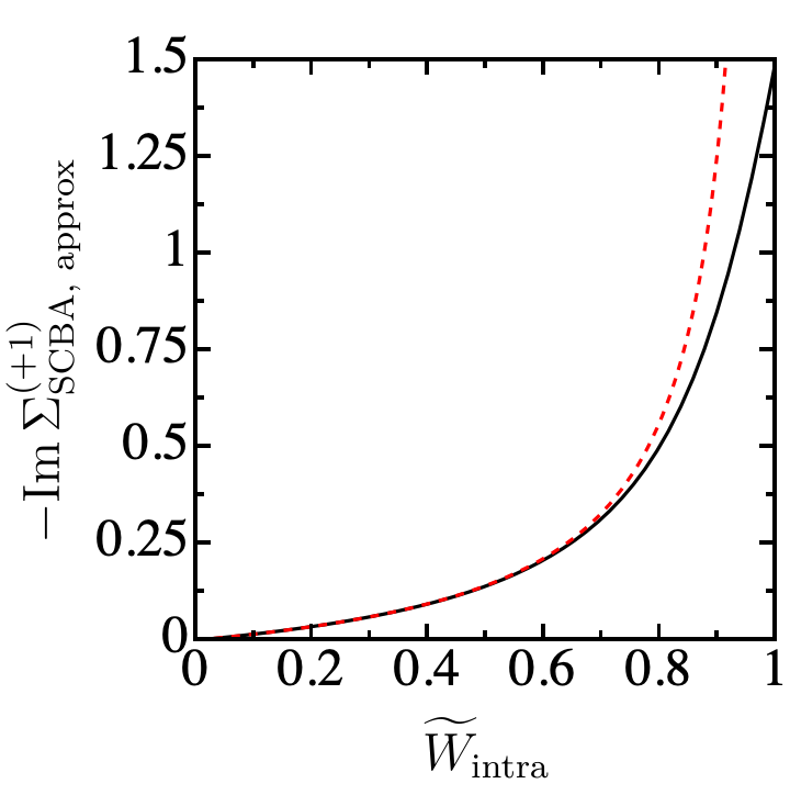
Figure 5: The black solid line represents the effective scattering strength $\Gamma=-\text{Im}\,\Sigma^{(\chi)}_{\text{SCBA, approx.}}$ evaluated at the frequency satisfying $\omega-\text{Re}\,\Sigma^{(\chi)}_{\text{SCBA, approx.}}(\omega)=\omega_{0}/2$ as a function of the dimensionless scattering strength $\widetilde{W}_{\text{intra}}$. The red dashed line shows the estimation from the approximate expression $\Gamma=\pi\,\widetilde{W}_{\text{intra}}\,\omega^{2}/2v_{F}\Lambda(1-\widetilde{W}_{\text{intra}})^{3}$ with $\omega=(1-\widetilde{W}_{\text{intra}})\omega_{0}/2$. The numerical parameters used are $v_{F}=1$, $\Lambda=25$, $\omega_{0}=3$.

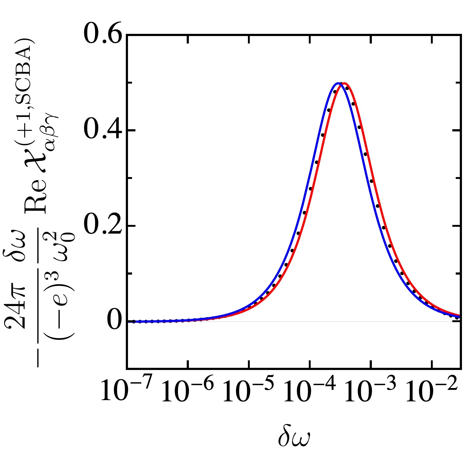
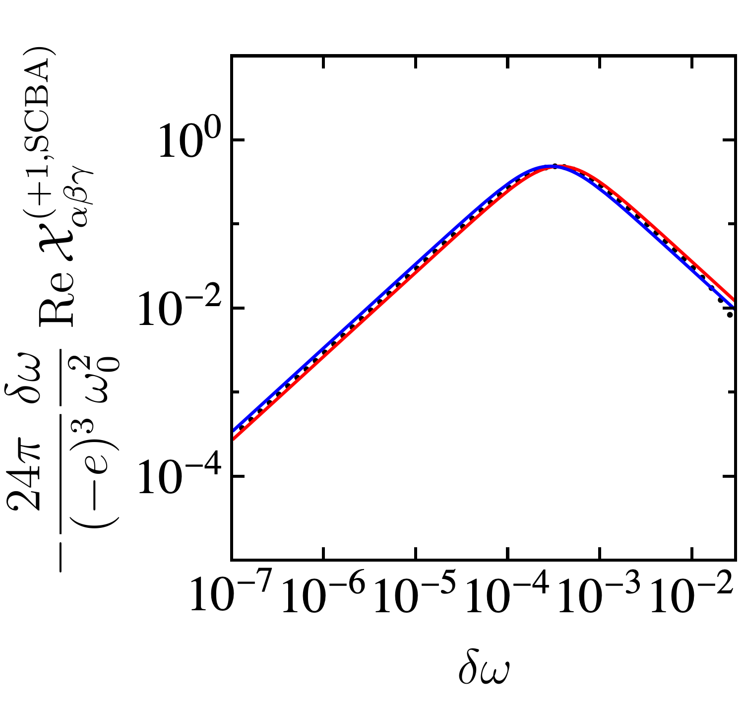
(a)     (b)
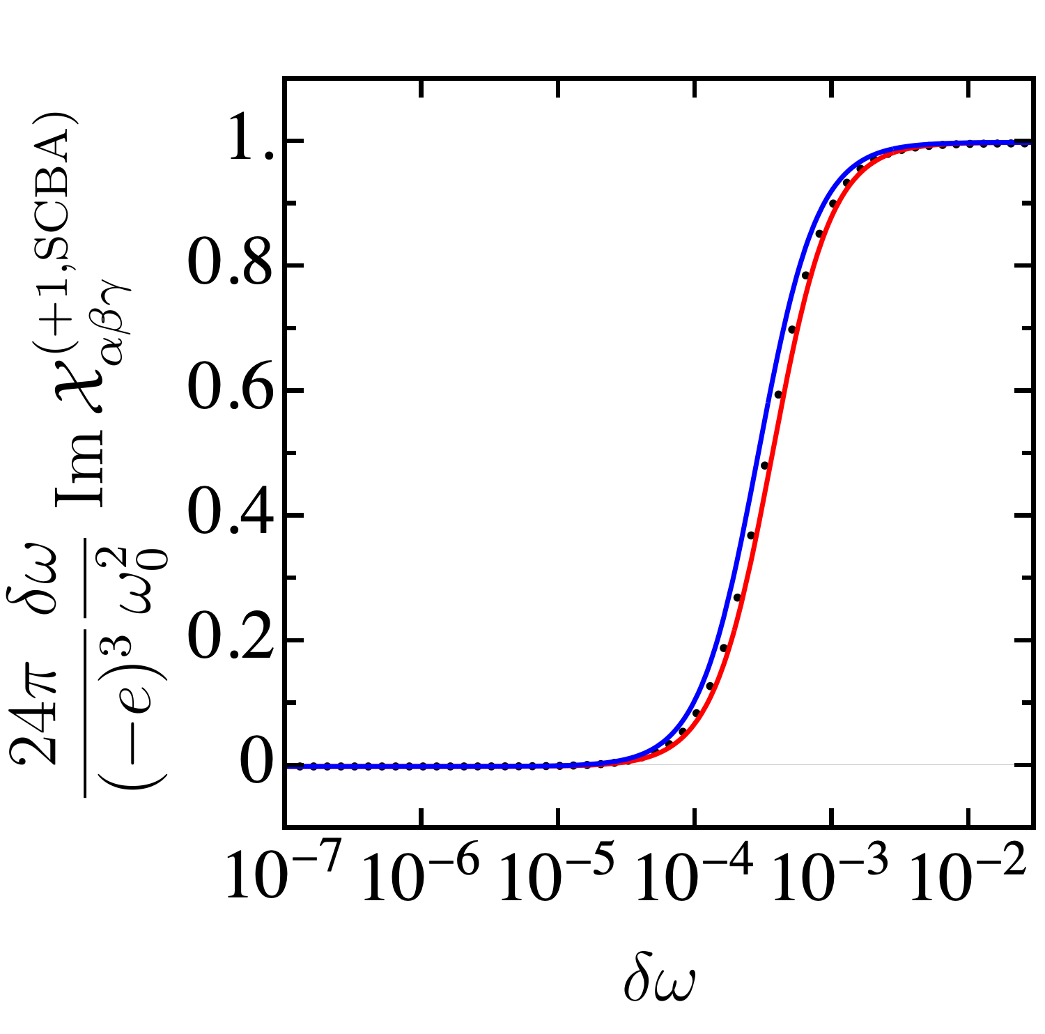
(c)     (d)

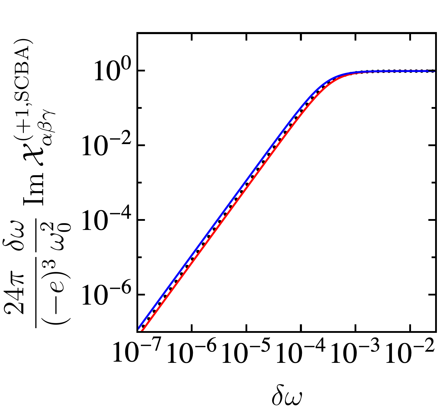
Figure 6: Panels (a) and (b) show the normalized real and imaginary parts of the response function $\mathcal{X}_{\alpha\beta\gamma}^{(+1,\text{SCBA})}\equiv\left.{\mathcal{X}}_{\alpha\beta\gamma}^{(+1,\text{SCBA})}(0,0;\omega_{0},-\omega_{0}+\delta\omega)\right|_{\widetilde{W}_{\text{inter}}=0}$ presented in Eq. (15) on linear scale as a function of the frequency detuning $\delta\omega$ in the absence of internode scattering. Panels (c) and (d) show the same data as (a) and (b) but on logarithmic scale. The black dots show the numerical evaluation of Eq. (15) with the replacements $i\Omega_{j}\to\omega_{j}+i\,\eta_{j}$, $\omega_{0}=3$, $\widetilde{W}_{\text{intra}}=10^{-3}$, $\mu_{1}=-1$, $v_{F}=1$, $\Lambda=25$, $\eta_{1}=1.05\cdot 10^{-5}$, $\eta_{2}=0.95\cdot 10^{-5}$, and $\eta=0.9\cdot 10^{-6}$. The red and blue lines depict the effective Drude-like expression in Eq. (17) when setting $\Gamma=-\text{Im}\,\Sigma^{(+1)}_{\text{SCBA, approx.}}$ and $\Gamma=\pi\,\widetilde{W}_{\text{intra}}\,\omega^{2}/2v_{F}\Lambda(1-\widetilde{W}_{\text{intra}})^{3}$ respectively.

VII Effect of internode scattering

In the presence of internode scattering, the numerical evaluation of Eq. (15) is performed similarly to the way outlined in Sec. VI, but with $\widetilde{W}_{\text{inter}}\neq 0$. We enforce Pauli-blocking at the Weyl node with $\chi=-1$ [17] by assuming that the corresponding energy offset $\mu_{-1}$ is sufficiently large compared to $\omega_{0}/2$, since impurity scattering tends to smear out (and thus modify) the current response around the onset in some frequency range around $2|\mu_{-1}|$. This would mix in an additional effect that would render the interpretation of our data less transparent. Figure  7 shows the effect of internode scattering on the optical response as defined in Eq. (15) as a function of $\widetilde{W}_{\text{intra}}$ for fixed ratios $\widetilde{W}_{\text{intra}}/\widetilde{W}_{\text{inter}}$. We find that due to the constant ratio of intra- and internode scattering, the value of $\widetilde{W}_{\text{intra}}$ can be viewed as a proxy for an effective larger scattering amplitude comprising the effects of $\widetilde{W}_{\text{intra}}$ and $\widetilde{W}_{\text{inter}}$. This scenario is thus in many ways similar to an effective intranode case with a rescaled scattering strength. We find that the entire optical response preserves many qualitative features of the Drude-like behavior even for strong internode scattering: the increased scattering leads to suppressed peak heights and broadened bandwidths for $\text{Re}\,\mathcal{X}$, and shifts of the entire response towards smaller scattering strengths. An interesting feature of Fig. 7 is the non-equidistant spacing between data points of different ratios $\widetilde{W}_{\text{intra}}/\widetilde{W}_{\text{inter}}$ indicating a non-linear scaling of $\mathcal{X}_{\alpha\beta\gamma}^{(+1,\text{SCBA})}$ as a function of the internode scattering strength. At fixed ratio $\widetilde{W}_{\text{inter}}/\widetilde{W}_{\text{intra}}=0.125$ but for varied energy offset $\mu_{-1}$ of the photo-idle Weyl node, Fig. 8 shows the entire optical response to be shifted towards smaller scattering strengths as the energy difference between the Weyl nodes grows, with Re$\mathcal{X}$ slightly distorted. In general, however, $\mathcal{X}_{\alpha\beta\gamma}^{(+1,\text{SCBA})}$ shows strong non-linear dependence on the energy difference between the Weyl nodes.

Figure  9 shows that when $\widetilde{W}_{\text{inter}}$ is fixed while $\widetilde{W}_{\text{intra}}$ is varied, the response function $\mathcal{X}_{\alpha\beta\gamma}^{(+1,\text{SCBA})}$ is reaching a non-zero plateau value depending on the strength of internode scattering when $\widetilde{W}_{\text{intra}}<\widetilde{W}_{\text{inter}}$. As far as $\text{Im}\,\mathcal{X}$ is concerned, the response and its plateau value depend more strongly on the strength of internode scattering compared to $\text{Re}\,\mathcal{X}$. This means that a regime with important internode scattering cannot be described in terms of our simple Drude-like behavior Eq. (17), which was derived in the absence of internode scattering. Moreover, Fig. 10 shows that non-zero plateau values for $\mathcal{X}_{\alpha\beta\gamma}^{(+1,\text{SCBA})}$ are also reached at small $\widetilde{W}_{\text{intra}}$ for varied $\mu_{-1}$ (at fixed $\widetilde{W}_{\text{inter}}$) and the suppression of the entire response due to increasing energy difference between the Weyl nodes is stronger compared to Fig. 9. Finally, we present Figs. 11 and 12 indicating that the increase of detuning frequency $\delta\omega$ tends to recover the quantized value for $\text{Im}\,\mathcal{X}$ (“CPGE-like quantization” – NB: the current in our case always oscillates periodically in time due to the finite detuning). However, similar to the discussion in Sec. VI, we expect that the impact of tuning $\delta\omega$ on the response function should depend on the optical frequency, and possibly also on other relevant system parameters such as the intra- and internode scattering strength and the energy difference between the Weyl nodes.

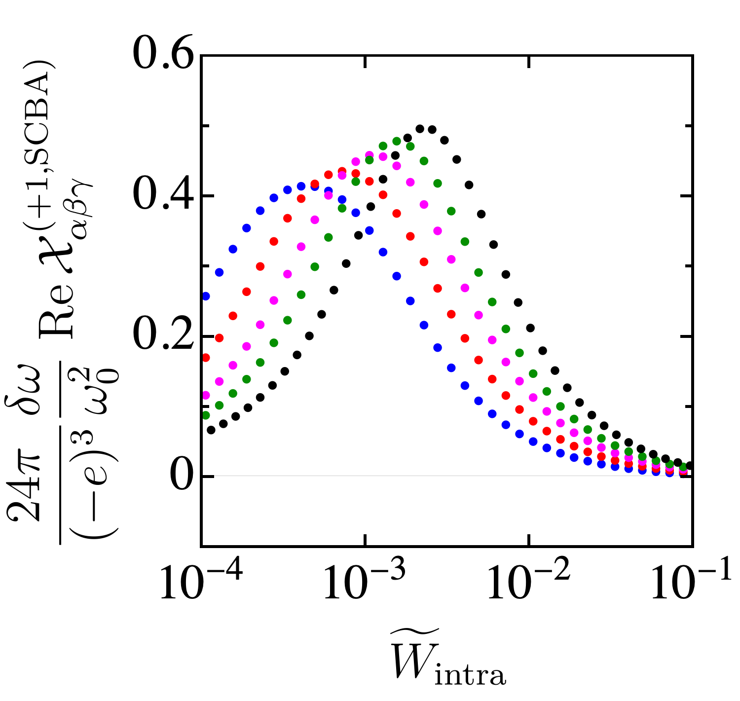
(a)     (b)

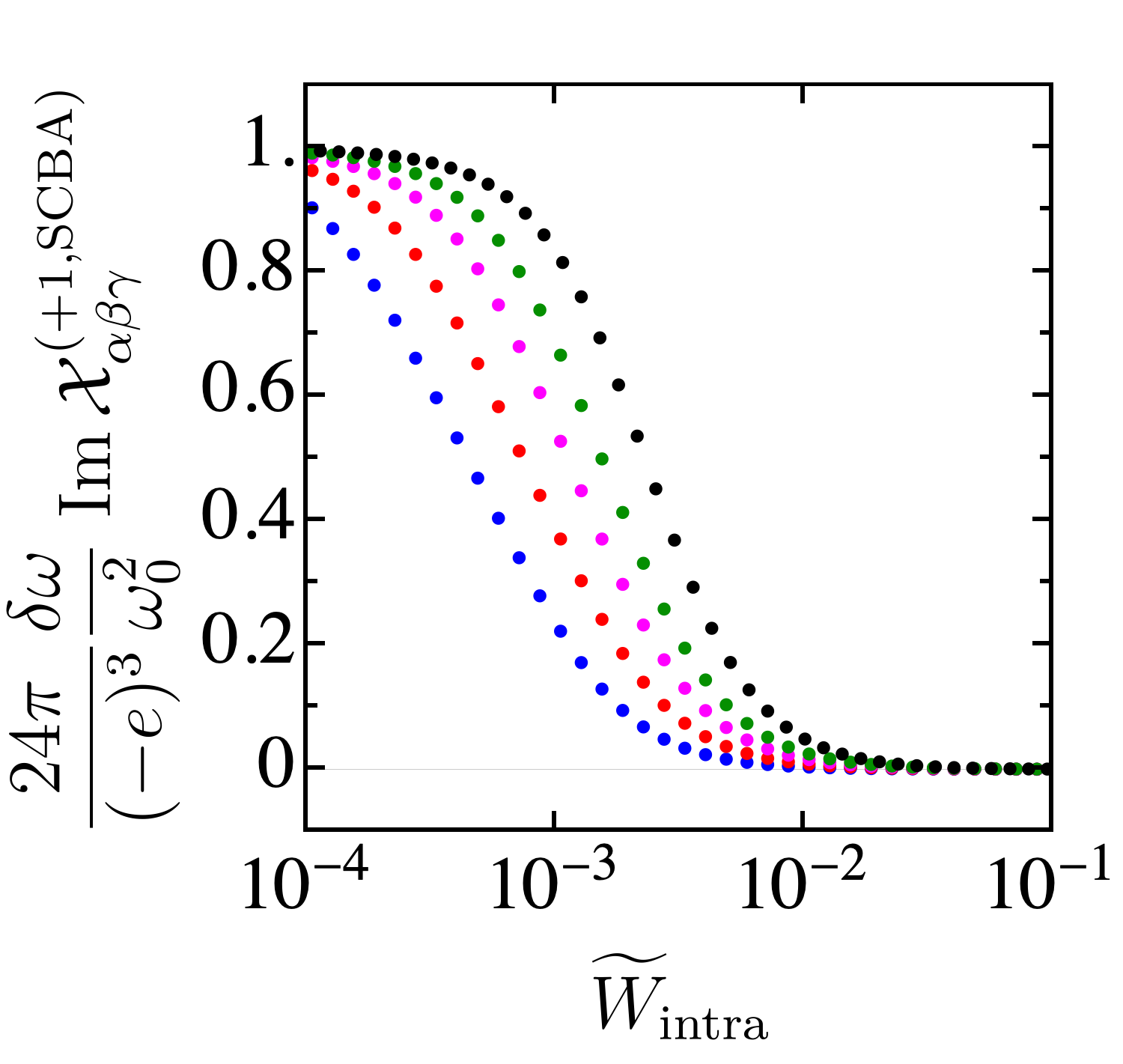
Figure 7: Panels (a) and (b) show the normalized real and imaginary parts of the response function $\mathcal{X}_{\alpha\beta\gamma}^{(+1,\text{SCBA})}\equiv{\mathcal{X}}_{\alpha\beta\gamma}^{(+1,\text{SCBA})}(0,0;\omega_{0},-\omega_{0}+\delta\omega)$ presented in Eq. (15) as a function of the dimensionless intranode scattering strength $\widetilde{W}_{\text{intra}}$ for four different scenarios for the ratio $x=\widetilde{W}_{\text{inter}}/\widetilde{W}_{\text{intra}}$: $x=1$ (blue dots), $x=0.5$ (red dots), $x=0.25$ (magenta dots) and $x=0.125$ (green dots). The black dos are the numerical data from Fig. 4 in the absence of internode scattering. For the numerical evaluation, we used in Eq. (15) the replacements $i\Omega_{j}\to\omega_{j}+i\,\eta_{j}$, $\omega_{1}=\omega_{0}$, $\omega_{2}=-\omega_{0}+\delta\omega$, $\omega_{0}=3$, $\mu_{1}=-1$, $v_{F}=1$, $\Lambda=25$, $\eta_{1}=1.05\cdot 10^{-5}$, $\eta_{2}=0.95\cdot 10^{-5}$, $\mu_{-1}=3$, $\eta=0.9\cdot 10^{-6}$ and $\delta\omega=10^{-3}$.

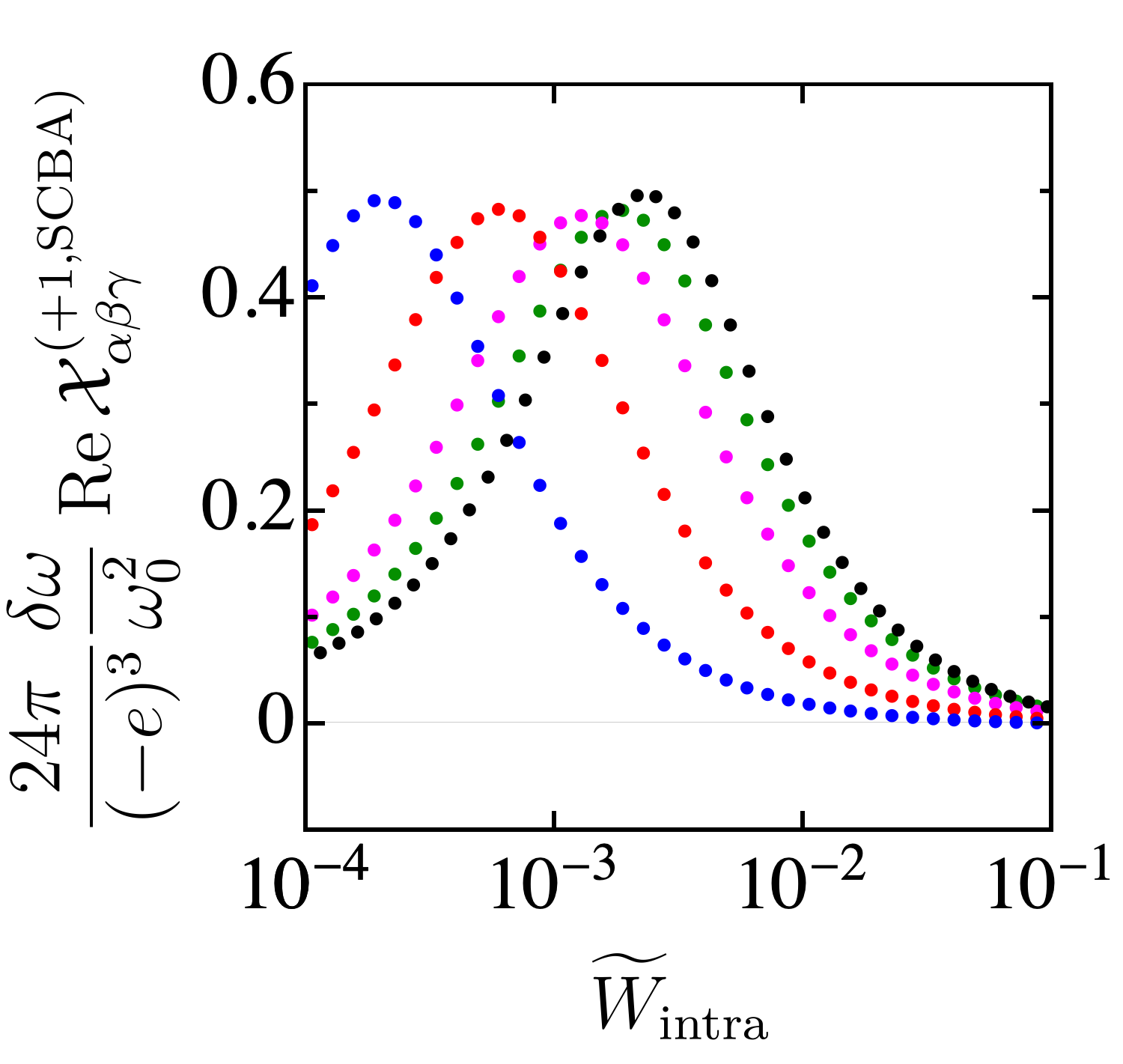
(a)     (b)

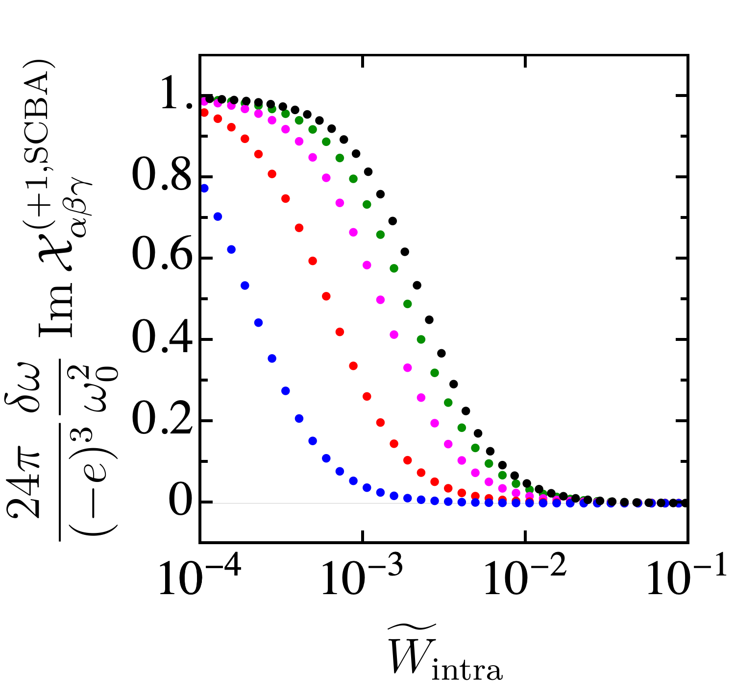
Figure 8: Panels (a) and (b) show the normalized real and imaginary parts of the response function $\mathcal{X}_{\alpha\beta\gamma}^{(+1,\text{SCBA})}\equiv{\mathcal{X}}_{\alpha\beta\gamma}^{(+1,\text{SCBA})}(0,0;\omega_{0},-\omega_{0}+\delta\omega)$ presented in Eq. (15) as a function of the dimensionless intranode scattering strength $\widetilde{W}_{\text{intra}}$ at fixed ratio $\widetilde{W}_{\text{inter}}/\widetilde{W}_{\text{intra}}=0.125$ for four different scenarios for the energy offset of the second Weyl node from the chemical potential: $\mu_{-1}=2$ (green dots), $\mu_{-1}=4$ (magenta dots), $\mu_{-1}=8$ (red dots) and $\mu_{-1}=16$ (blue dots). The black dots are the numerical data from Fig. 4 in the absence of internode scattering. The numerical evaluation is done using the same rest of parameters as Fig. 7.

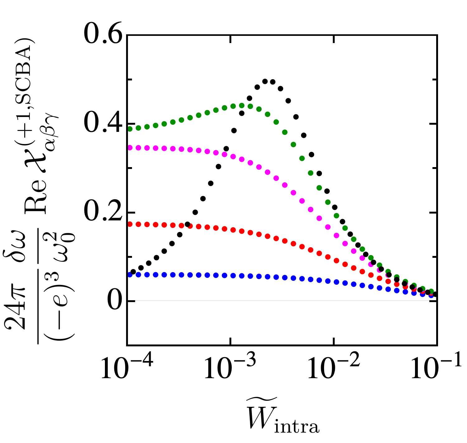
(a)     (b)

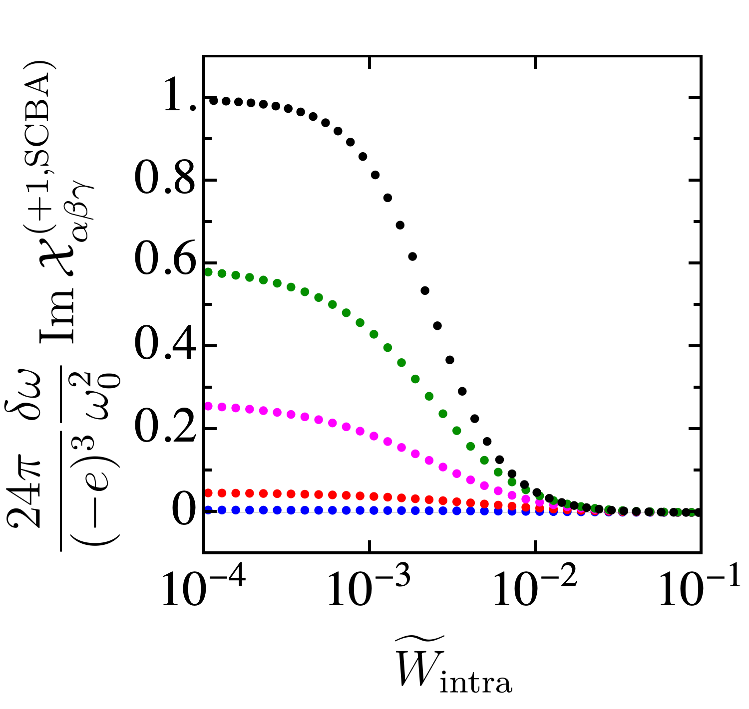
Figure 9: Panels (a) and (b) show the normalized real and imaginary parts of the response function $\mathcal{X}_{\alpha\beta\gamma}^{(+1,\text{SCBA})}\equiv{\mathcal{X}}_{\alpha\beta\gamma}^{(+1,\text{SCBA})}(0,0;\omega_{0},-\omega_{0}+\delta\omega)$ presented in Eq. (15) as a function of the dimensionless intranode scattering strength $\widetilde{W}_{\text{intra}}$ for four different scenarios of internode scattering strength $\widetilde{W}_{\text{inter}}$ at fixed $\mu_{-1}=3$: $\widetilde{W}_{\text{inter}}=10^{-3.5}$ (green dots), $\widetilde{W}_{\text{inter}}=10^{-3}$ (magenta dots), $\widetilde{W}_{\text{inter}}=10^{-2.5}$ (red dots) and $\widetilde{W}_{\text{inter}}=10^{-2}$ (blue dots). The black dots are the numerical data from Fig. 4 in the absence of internode scattering. The numerical evaluation is done using the same values as the plots in the first row in Fig. 7 for all remaining parameters.

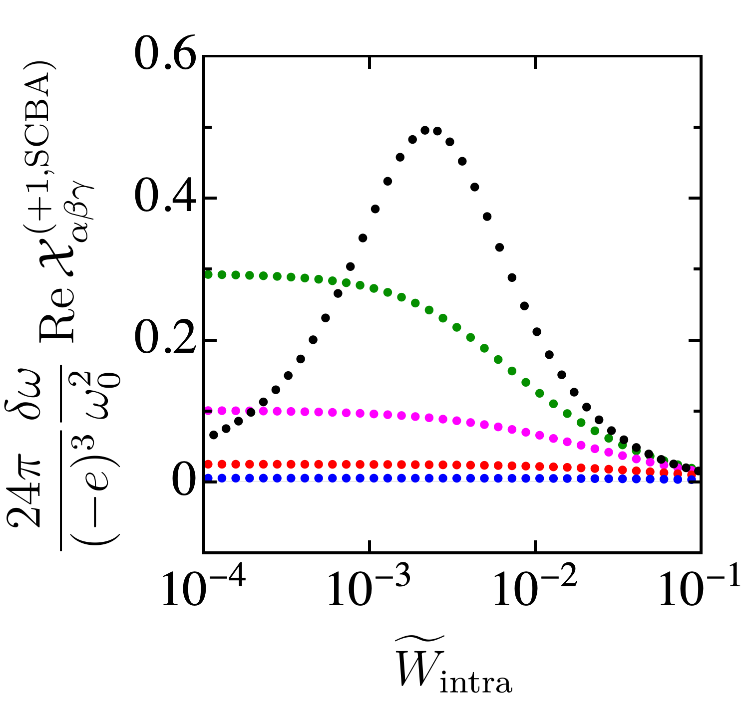
(a)     (b)

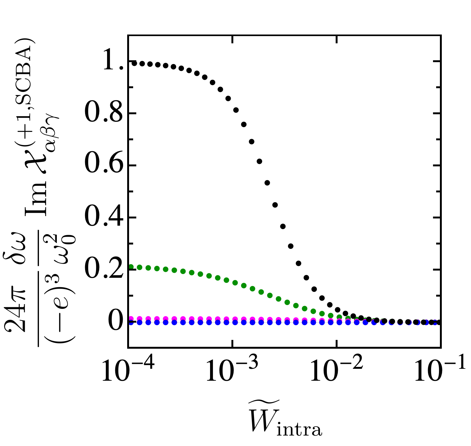
Figure 10: Panels (a) and (b) show the normalized real and imaginary parts of the response function $\mathcal{X}_{\alpha\beta\gamma}^{(+1,\text{SCBA})}\equiv{\mathcal{X}}_{\alpha\beta\gamma}^{(+1,\text{SCBA})}(0,0;\omega_{0},-\omega_{0}+\delta\omega)$ presented in Eq. (15) as a function of the dimensionless intranode scattering strength $\widetilde{W}_{\text{intra}}$ for four different scenarios for the energy offset of the second Weyl node from the chemical potential at fixed internode scattering strength $\widetilde{W}_{\text{inter}}=10^{-3}$: $\mu_{-1}=2$ (green dots), $\mu_{-1}=4$ (magenta dots), $\mu_{-1}=8$ (red dots) and $\mu_{-1}=16$ (blue dots). The black dots are the numerical data from Fig. 4 in the absence of internode scattering. The numerical evaluation is done using the same values as the plots in the first row in Fig. 7 for all remaining parameters.

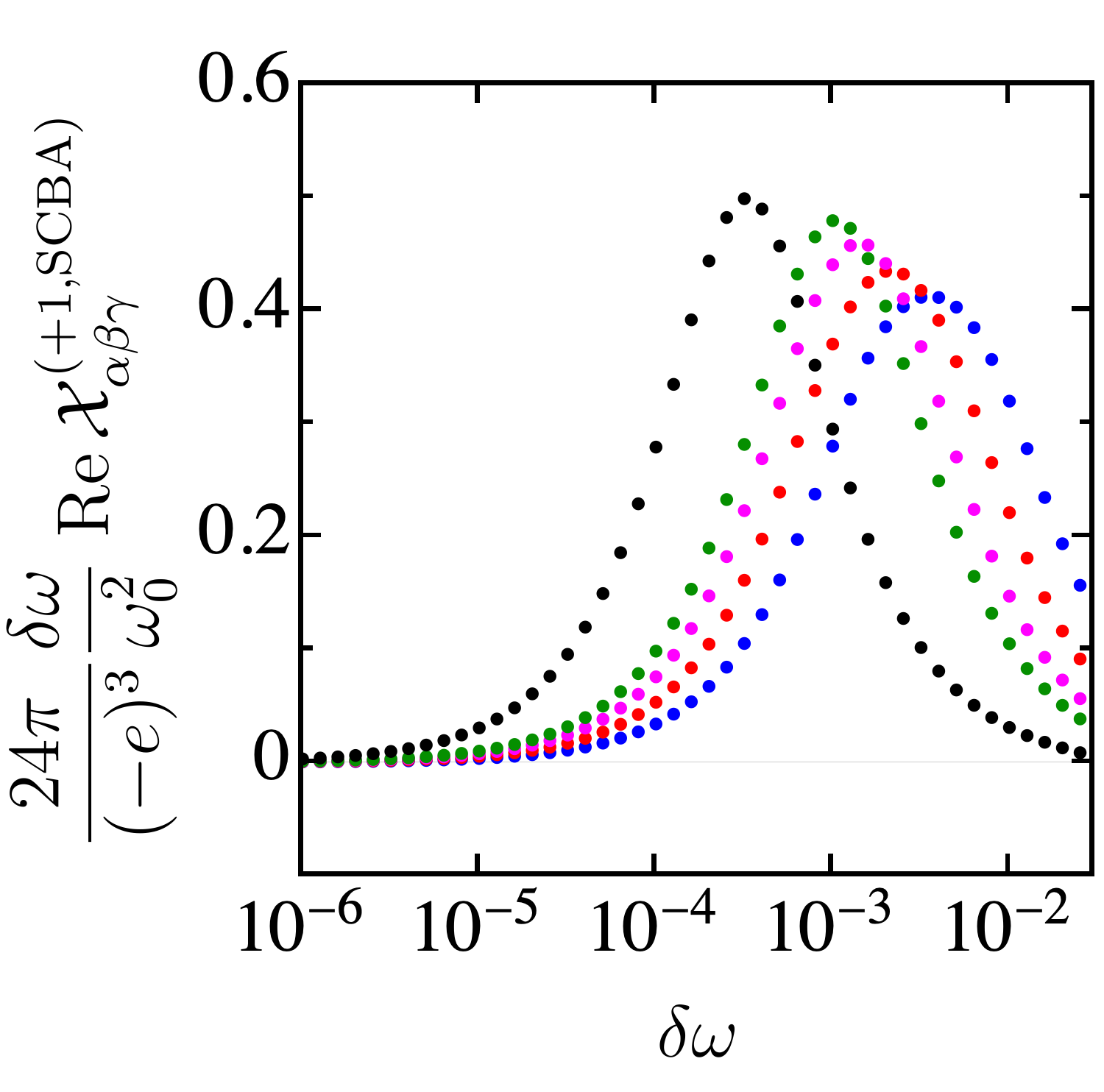
(a)     (b)

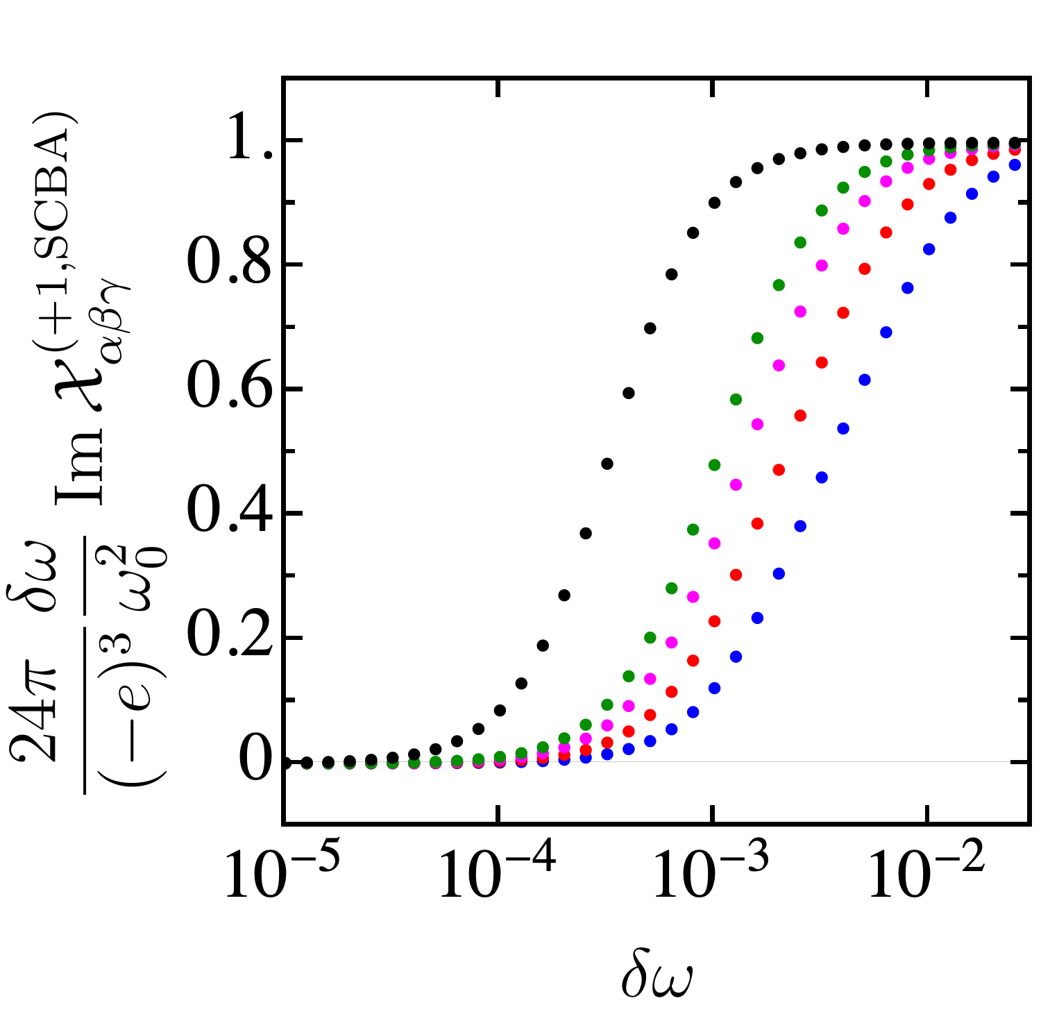
Figure 11: Panels (a) and (b) show the normalized real and imaginary parts of the response function $\mathcal{X}_{\alpha\beta\gamma}^{(+1,\text{SCBA})}\equiv{\mathcal{X}}_{\alpha\beta\gamma}^{(+1,\text{SCBA})}(0,0;\omega_{0},-\omega_{0}+\delta\omega)$ presented in Eq. (15) as a function of the frequency detuning $\delta\omega$ at $\mu_{-1}=3$ for four different scenarios for the ratio $x=\widetilde{W}_{\text{inter}}/\widetilde{W}_{\text{intra}}$: $x=1$ (blue dots), $x=0.5$ (red dots), $x=0.25$ (magenta dots) and $x=0.125$ (green dots). The black dots are the numerical data from Fig. 4 in the absence of internode scattering.For the numerical evaluation, we used in Eq. (15) the replacements $i\Omega_{j}\to\omega_{j}+i\,\eta_{j}$, $\omega_{1}=\omega_{0}$, $\omega_{2}=-\omega_{0}+\delta\omega$, $\omega_{0}=3$, $\mu_{1}=-1$, $v_{F}=1$, $\Lambda=25$, $\eta_{1}=1.05\cdot 10^{-5}$, $\eta_{2}=0.95\cdot 10^{-5}$, $\eta=0.9\cdot 10^{-6}$ and $\widetilde{W}_{\text{intra}}=10^{-3}$.

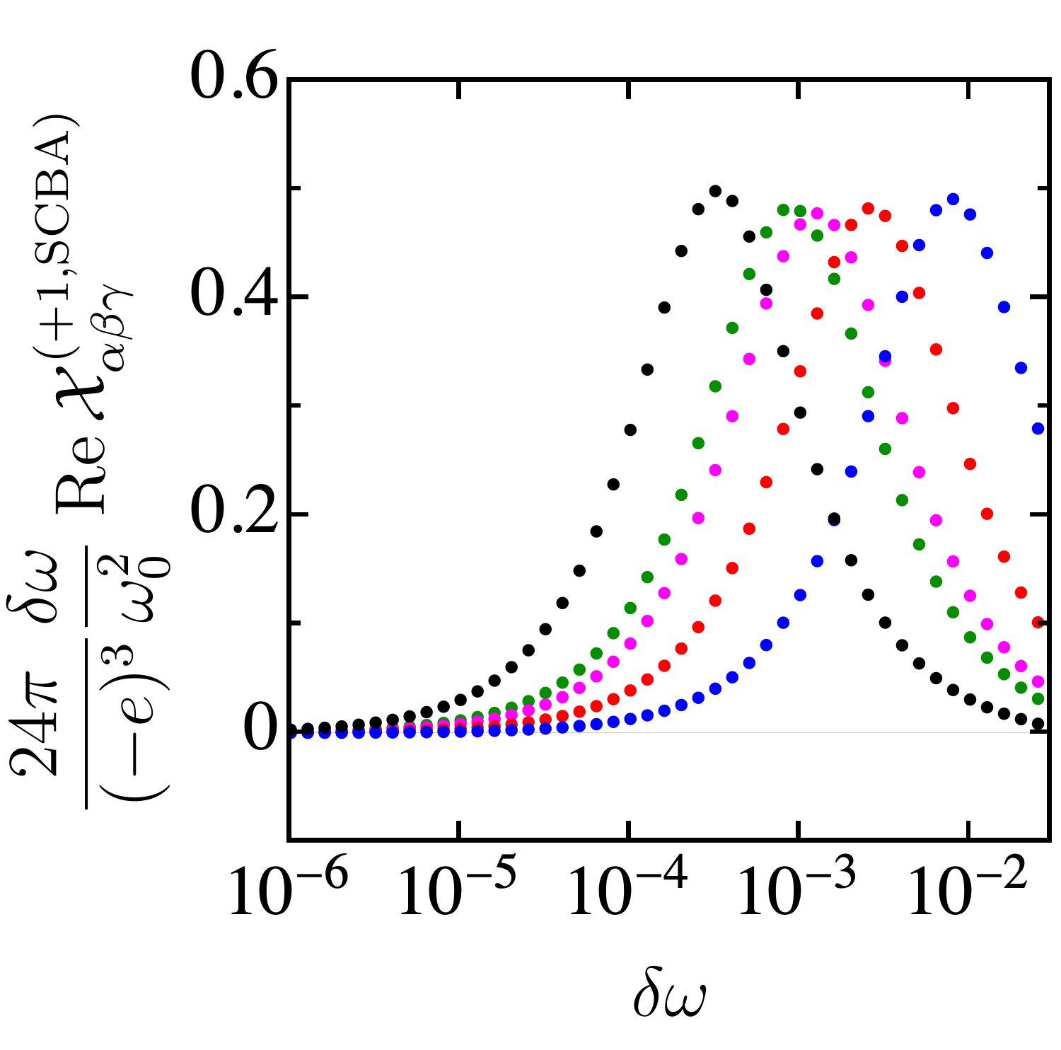
(a)     (b)

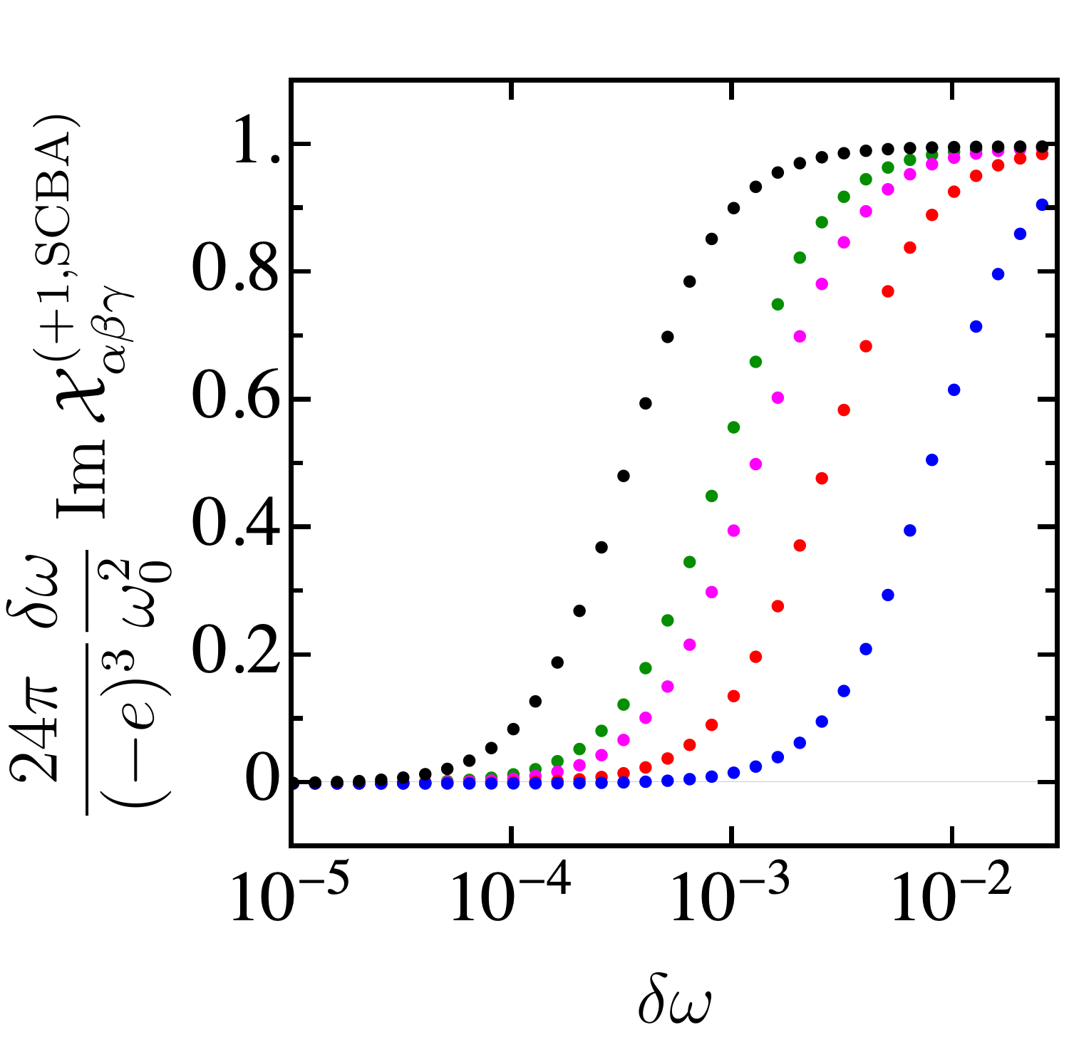
Figure 12: Panels (a) and (b) show the normalized real and imaginary parts of the response function $\mathcal{X}_{\alpha\beta\gamma}^{(+1,\text{SCBA})}\equiv{\mathcal{X}}_{\alpha\beta\gamma}^{(+1,\text{SCBA})}(0,0;\omega_{0},-\omega_{0}+\delta\omega)$ presented in Eq. (15) as a function of the detuning frequency $\delta\omega$ for fixed ratio $\widetilde{W}_{\text{inter}}/\widetilde{W}_{\text{intra}}=0.125$ for four different scenarios for the energy offset of the second Weyl node from the chemical potential: $\mu_{-1}=2$ (green dots), $\mu_{-1}=4$ (magenta dots), $\mu_{-1}=8$ (red dots) and $\mu_{-1}=16$ (blue dots). The black dots are the numerical data from Fig. 4 in the absence of internode scattering. The numerical evaluation is done using the same values as the plots in the first row in Fig. 11 for all remaining parameters.

VIII Summary and outlook

In summary, we have generalized the second-order optical response of CPGE in the presence of finite frequency detuning on a system with two Weyl nodes located at different energies. We considered the behavior of the real and imaginary parts of the corresponding correlation function in terms of elastic impurity intra- and internode scattering processes, frequency detuning, and energy difference between the two Weyl nodes. We have presented numerical data in Figs. (4)-(5) substantiated by the effective model for the scattering strength defined in Eq. (17) suggesting that the optical response as function of intranode scattering is qualitatively similar to the Drude-like behavior of the AC linear optical conductivity in metals. As long as intra- and internode scattering strengths have a fixed ratio, the Drude-like characteristics of the optical response are preserved, see Figs. (7) and (8). However, when the internode scattering strength is kept fixed while the intranode scattering strength varies, the response function deviates strongly from the Drude-like behavior and shows non-zero plateau values for both real and imaginary parts in the limit of weak intranode scattering, see Figs. (9)-(10). We have also presented data in Figs. (6), (11) and (12) suggesting that the imaginary part of the response function can reach a “quantized” value when the frequency detuning is properly adjusted.

We conclude the present paper with an outlook on the experimental relevance of our findings. First of all, the decisive qualitative and quantitative consequences of finite frequency detuning on the second-order CPGE optical response make the case that non-trivial dependence can be probed by all externally controlled parameters, namely frequency detuning, optical frequency, energy difference between the Weyl nodes and doping. Moreover, measuring the amplitude and phase shift of the current density with respect to the applied electric field, one can determine the real and imaginary parts of the response, and hence by comparing to our results the effective scattering strength $\Gamma$ - at least in a regime where Eq. (17) is valid. Candidate materials where such experimental probes can be implemented are transition metal monopnictides (TMMPs) such as TaAs, TaP and NbAs. TMMPs have already been used to identify the existence of CPGE in Weyl semimetals (TaAs) through the measurement of the helicity-dependent generated voltage [24], to probe the giant nonlinear response associated to the second harmonic generation (SHG) [33], and to detect the chirality of Weyl fermions through the CPGE response using mid-infrared optical frequency [23]. Furthermore, it would be interesting to see the features of the generalized CPGE optical response we have predicted to get tested in other materials as well, such as heterostructures [34], alloys [35] and half-Heusler compounds [36], in which a minimal model of a pair of Weyl nodes has been theoretically proposed. However, we expect our findings to be applicable also to materials with multiple pairs of Weyl nodes, provided they are well separated in momentum space.

Appendix A Summary of quadratic response theory

We here provide a short review of how the second-order generalization of the optical conductivity can be derived. One begins by expanding the electric current operator $\bm{j}$ in orders of the applied electromagnetic fields [37, 38]. When the velocity gauge is used [39], the expansion yields $\bm{j}=\sum_{n}\bm{j}^{(n)}$ with $\bm{j}^{(n)}=(e/\hbar n!)\widehat{D}^{\alpha_{0}}\prod_{i=1}^{n}(eA^{\alpha_{i}}\widehat{D}^{\alpha_{i}}/\hbar)$ being the $n$th order current density operator defined in terms of the electromagnetic vector potential $A^{\alpha_{i}}$ and covariant derivative $\widehat{D}^{\alpha_{i}}$, where $\alpha_{i}\in\{x,y,z\}$ is a spatial index. While the diamagnetic term in the current density of a free electron gas is a well-known example for $\bm{j}^{(1)}$, lattice Hamiltonians generically feature contributions at all orders $n$. Suppressing integrations, prefactors, spacetime-arguments, and indices for simplicity, the total “second order current” can schematically be expressed as

$$\begin{split}\langle\bm{j}(\bm{r},t)\rangle_{\text{quadr.}}=&\langle\bm{j}^{(2)}\rangle_{0}+\langle[\bm{j}^{(1)},H_{\rm pert}^{(1)}]\rangle_{0}+\langle[\bm{j}^{(0)},H_{\rm pert}^{(2)}]\rangle_{0}\\ &+\langle[\bm{j}^{(0)},[H_{\rm pert}^{(1)},H_{\rm pert}^{(1)}]]\rangle_{0},\end{split}$$ (20)

where $\langle\cdot\rangle_{0}$ denotes an expectation value with respect to $H_{0}$, the time-independent Hamiltonian in the absence of electromagnetic fields, and where $H_{\rm pert}^{(n)}=-\bm{j}^{(n-1)}\cdot\bm{A}$. The term $\langle\bm{j}^{(2)}\rangle_{0}$ is called ”Drude weight dipole” whereas the rest of terms correspond to one- and two-photon resonances. The CPGE of a Weyl semimetal is a part of the current deriving from the term $\langle[\bm{j}^{(0)},[H_{\rm pert}^{(1)},H_{\rm pert}^{(1)}]]\rangle_{0}$ [39].

Similarly to linear response theory, quadratic response can also be understood as describing the temporal dynamics of equilibrium systems in the presence of weak, time-dependent external fields long after the perturbation has been switched on. One can therefore conveniently connect the response function underlying the CPGE to equilibrium Matsubara Green’s functions. Restoring all notational details, and adopting the velocity gauge after approximating the model to its low-energy form, the response containing the CPGE alongside other quadratic responses such as second harmonic generation can be written as [40]

$$\langle j_{\alpha}(\bm{r},t)\rangle^{\text{(CPGE+other)}}=\int_{-\infty}^{\infty}dt^{\prime}\int d^{3}r^{\prime}\int_{-\infty}^{\infty}dt\int d^{3}r^{\prime\prime}\,\sum_{\beta,\gamma}\,X_{\alpha\beta\gamma}(\bm{r}-\bm{r^{\prime}},\bm{r}-\bm{r}^{\prime\prime};t-t^{\prime},t-t^{\prime\prime})\,A_{\beta}(\bm{r}^{\prime},t^{\prime})\,A_{\gamma}(\bm{r}^{\prime\prime},t^{\prime\prime}),$$ (21)

where $\alpha,\beta,\gamma\in\{x,y,z\}$, and

$$X_{\alpha\beta\gamma}(\bm{r}-\bm{r^{\prime}},\bm{r}-\bm{r}^{\prime\prime};t-t^{\prime},t-t^{\prime\prime}) =-\theta(t-t^{\prime})\theta(t^{\prime}-t^{\prime\prime})\,\langle\left[\left[j_{\alpha}(\bm{r},t),j_{\beta}(\bm{r}^{\prime},t^{\prime})\right],j_{\gamma}(\bm{r}^{\prime\prime},t^{\prime\prime})\right]\rangle_{0}.$$ (22)

The response function $X_{\alpha\beta\gamma}$ can be symmetrized by relabeling $\beta\leftrightarrow\gamma$, $t^{\prime}\leftrightarrow t^{\prime\prime}$ and $\bm{r}^{\prime}\leftrightarrow\bm{r}^{\prime\prime}$, and averaging $X_{\alpha\beta\gamma}$ and the relabeled $X_{\alpha\beta\gamma}$. For spatiotemporally translation-invariant systems, the Fourier transform of the symmetrized response function

$$\mathcal{X}_{\alpha\beta\gamma}(\bm{q}_{1},\bm{q}_{2};\omega_{1},\omega_{2})=\int d^{3}r_{1}\int dt_{1}\int d^{3}r_{2}\int dt_{2}\,e^{-i(\bm{q}_{1}\cdot\bm{r}_{1}-\omega_{1}t_{1})}e^{-i(\bm{q}_{2}\cdot\bm{r}_{2}-\omega_{2}t_{2})}\,\frac{X_{\alpha\beta\gamma}(\bm{r}_{1},\bm{r}_{2};t_{1},t_{2})+X_{\alpha\gamma\beta}(\bm{r}_{2},\bm{r}_{1};t_{2},t_{1})}{2}$$ (23)

can via Lehmann representation be connected to

$$\mathcal{X}_{\alpha\beta\gamma}(\bm{q}_{1},\bm{q}_{2};\omega_{1},\omega_{2})=\frac{1}{2}\,\left.\tilde{\mathcal{X}}_{\alpha\beta\gamma}(\bm{q}_{1},\bm{q}_{2};i\Omega_{1},i\Omega_{2})\right|_{i\Omega_{j}\to\omega_{j}+i\,\eta_{j}},$$ (24)

where $\Omega_{j}$ are (bosonic) Matsubara frequencies and $\eta_{j}\to 0^{+}$, while $\tilde{\mathcal{X}}_{\alpha\beta\gamma}$ is defined as

$$\tilde{\mathcal{X}}_{\alpha\beta\gamma}(\bm{q}_{1},\bm{q}_{2};i\Omega_{1},i\Omega_{2}) =\int d^{3}r_{1}\int_{0}^{\beta}d\tau_{1}\int d^{3}r_{2}\int_{0}^{\beta}d\tau_{2}\,e^{-i(\bm{q}_{1}\cdot\bm{r}_{1}-\Omega_{1}\tau_{1})}e^{-i(\bm{q}_{2}\cdot\bm{r}_{2}-\Omega_{2}\tau_{2})}\,\tilde{X}_{\alpha\beta\gamma}(\bm{r}_{1},\bm{r}_{2};\tau_{1},\tau_{2}),$$ (25)

$$\tilde{X}_{\alpha\beta\gamma}(\bm{r}_{1},\bm{r}_{2};\tau_{1},\tau_{2}) =\langle T_{\tau}\,\tilde{j}_{\alpha}(0,0)\,\tilde{j}_{\beta}(-\bm{r}_{1},-\tau_{1})\,\tilde{j}_{\gamma}(-\bm{r}_{2},-\tau_{2})\rangle.$$ (26)

Here, tildes indicate quantities depending on imaginary time or Matsubara frequencies with the Heisenberg picture implying $\tilde{j}_{\alpha}(\bm{r},\tau=0)={j}_{\alpha}(\bm{r},t=0)={j}_{\alpha}(\bm{r})$. Finally, we specialize to a situation in which the electromagnetic field corresponds to a collection of spatially homogeneous electric fields at frequencies $\nu_{j}$, i.e. $\bm{E}(t)=\sum_{j}\bm{E}_{j}\,e^{-i\nu_{j}t}$. In the velocity gauge, we then find

$$\langle j_{\alpha}(\bm{r},t)\rangle^{\text{(CPGE+other)}}=-\sum_{j,k}\sum_{\beta,\gamma}\,\frac{1}{\nu_{j}\,\nu_{k}}\mathcal{X}_{\alpha\beta\gamma}(0,0;\nu_{j},\nu_{k})\,E_{j,\beta}\,E_{k,\gamma}\,e^{i(\nu_{j}+\nu_{k})t}.$$ (27)

Note that $X_{\alpha\beta\gamma}(\bm{r}_{1},\bm{r}_{2};t_{1},t_{2})$ is a real-valued function, such that $\mathcal{X}_{\alpha\beta\gamma}(0,0;\nu_{j},\nu_{k})=\mathcal{X}_{\alpha\beta\gamma}(0,0;-\nu_{j},-\nu_{k})^{*}$. In addition, in the low-energy regime of a Weyl semimetal described by purely linearly dispersing bands, the current density operator is $\bm{j}=\bm{j}^{(0)}$, such that all other contributions in to the quadratic response $\langle j_{\alpha}(\bm{r},t)\rangle^{\text{(quad.)}}$ vanish. Therefore, in the main text we use $\langle j_{\alpha}(\bm{r},t)\rangle^{\text{(quad.)}}=\langle j_{\alpha}(\bm{r},t)\rangle^{\text{(CPGE+other)}}$.

Appendix B Intermediate results for the Drude-like form of the response function

Our starting point is the expression of ${\mathcal{X}}_{\alpha\beta\gamma}^{(\chi,\text{SCBA})}$ in Eq. (15) after approximating self-energies and vertex corrections as described in the main text. We then approximate factors of Lorentzian spectral density of states by delta-peaks, $\rho(\omega)=\Gamma/(\pi(\omega^{2}+\Gamma^{2}))\to\delta(\omega)$, which allows us to perform the frequency integration. This yields

$$\left.{\mathcal{X}}_{\alpha\beta\gamma}^{(\chi,\text{SCBA})}(0,0;\omega_{1},\omega_{2})\right|_{\widetilde{W}_{\text{inter}}=0}\approx\frac{i}{12\,\pi^{2}}\chi\epsilon^{\alpha\beta\gamma}(-e)^{3}v_{F}^{3}\int_{0}^{\Lambda}dkk^{2}\sum_{b_{1},b_{2},b_{3}=\pm 1}\tilde{\delta}_{b_{1},b_{2},b_{3}}$$

$$\times\Biggl{(}\frac{n_{F}(b_{3}v_{F}k+|\mu_{\chi}|)}{\omega_{1}+\omega_{2}+(b_{3}-b_{1})v_{F}k+i\,\Gamma}\,\frac{1}{\omega_{2}+(b_{3}-b_{2})v_{F}k+i\,\Gamma}+\frac{n_{F}(b_{2}v_{F}k+|\mu_{\chi}|)}{\omega_{1}+(b_{2}-b_{1})v_{F}k+i\,\Gamma}\,\frac{1}{-\omega_{2}+(b_{2}-b_{3})v_{F}k-i\,\Gamma}$$

$$+\frac{n_{F}(b_{1}v_{F}k+|\mu_{\chi}|)}{-\omega_{1}+(b_{1}-b_{2})v_{F}k-i\,\Gamma}\,\frac{1}{-\omega_{1}-\omega_{2}+(b_{1}-b_{3})v_{F}k-i\,\Gamma}\Biggr{)}+(\beta\leftrightarrow\gamma,\omega_{1}\leftrightarrow\omega_{2}).$$ (28)

We then take the limit of zero temperature, and introduce $Q=2v_{F}k$ and $\tilde{\Lambda}=2v_{F}\Lambda$. Then performing the sum over $b_{j}$’s and regrouping terms yields

$$\left.{\mathcal{X}}_{\alpha\beta\gamma}^{(\chi,\text{SCBA})}(0,0;\omega_{1},\omega_{2})\right|_{\widetilde{W}_{\text{inter}}=0}\approx\frac{i}{96\,\pi^{2}}\chi\epsilon^{\alpha\beta\gamma}(-e)^{3}\int_{2|\mu_{\chi}|}^{\tilde{\Lambda}}dQ\,Q^{2}$$

$$\times\Biggl{(}\frac{1}{Q-(\omega_{1}+\omega_{2}+i\Gamma)}\,\frac{1}{Q-(\omega_{2}+i\Gamma)}-\left(1-\frac{i\Gamma}{\omega_{1}+i\Gamma}\right)\,\frac{1}{Q+(\omega_{1}+\omega_{2}+i\Gamma)}\,\frac{1}{Q+(\omega_{2}+i\Gamma)}$$

$$+\frac{1}{Q-(\omega_{1}+i\Gamma)}\,\frac{1}{Q+(\omega_{2}+i\Gamma)}-\left(1+\frac{i\Gamma}{\omega_{1}+\omega_{2}+i\Gamma}\right)\,\frac{1}{Q+(\omega_{1}+i\Gamma)}\,\frac{1}{Q-(\omega_{2}+i\Gamma)}$$

$$+\frac{1}{Q+(\omega_{1}+\omega_{2}+i\Gamma)}\,\frac{1}{Q-(\omega_{1}+i\Gamma)}-\left(1-\frac{i\Gamma}{\omega_{2}+i\Gamma}\right)\,\frac{1}{Q-(\omega_{1}+\omega_{2}+i\Gamma)}\,\frac{1}{Q-(\omega_{1}+i\Gamma)}\Biggr{)}+(\beta\leftrightarrow\gamma,\omega_{1}\leftrightarrow\omega_{2}).$$ (29)

We simplify this expression assuming that $\Gamma\ll|\omega_{1}|$, $|\omega_{2}|$, $|\omega_{1}+\omega_{2}|$. We can then drop the fractions in the brackets. In addition, we assume that the cutoff is large such that $\tilde{\Lambda}\gg|\omega_{1}|$, $|\omega_{2}|$, $|\omega_{1}+\omega_{2}|$. We then find

$$\left.{\mathcal{X}}_{\alpha\beta\gamma}^{(\chi,\text{SCBA})}(0,0;\omega_{1},\omega_{2})\right|_{\widetilde{W}_{\text{inter}}=0}\approx\frac{i}{96\,\pi^{2}}\chi\epsilon^{\alpha\beta\gamma}(-e)^{3}$$

$$\times\Biggl{(}\frac{(\omega_{1}+\omega_{2}+i\Gamma)^{2}}{\omega_{2}}\ln\left(4|\mu_{\chi}|^{2}-(\omega_{1}+\omega_{2}+i\Gamma)^{2}\right)-\frac{(\omega_{1}+\omega_{2}+i\Gamma)^{2}}{\omega_{1}}\ln\left(4|\mu_{\chi}|^{2}-(\omega_{1}+\omega_{2}+i\Gamma)^{2}\right)$$

$$+\frac{(\omega_{2}+i\Gamma)^{2}}{\omega_{1}+\omega_{2}+2i\Gamma}\ln\left(4|\mu_{\chi}|^{2}-(\omega_{2}+i\Gamma)^{2}\right)-\frac{(\omega_{1}+i\Gamma)^{2}}{\omega_{1}+\omega_{2}+2i\Gamma}\ln\left(4|\mu_{\chi}|^{2}-(\omega_{1}+i\Gamma)^{2}\right)$$

$$+\frac{(\omega_{2}+i\Gamma)^{2}}{\omega_{1}}\ln\left(4|\mu_{\chi}|^{2}-(\omega_{2}+i\Gamma)^{2}\right)-\frac{(\omega_{1}+i\Gamma)^{2}}{\omega_{2}}\ln\left(4|\mu_{\chi}|^{2}-(\omega_{1}+i\Gamma)^{2}\right)\Biggr{)}+(\beta\leftrightarrow\gamma,\omega_{1}\leftrightarrow\omega_{2}).$$ (30)

It is now obvious that the term $(\beta\leftrightarrow\gamma,\omega_{1}\leftrightarrow\omega_{2})$ simply corresponds to a factor of two. We specify $\omega_{1}=\omega_{0}$, $\omega_{2}=-\omega_{0}+\delta\omega$, and assume $|\delta\omega|\ll|\omega_{0}|$. We furthermore recall the assumption $\Gamma\ll|\delta\omega|$. The response function is therefore dominated by the terms $\sim(\omega_{1}+\omega_{2}+i\Gamma)^{-1}$. Furthermore approximating $\omega_{0}\pm i\Gamma\approx\omega_{0}$ in the prefactors of the logarithm yields

$$\left.{\mathcal{X}}_{\alpha\beta\gamma}^{(\chi,\text{SCBA})}(0,0;\omega_{0},-\omega_{0}+\delta\omega)\right|_{\widetilde{W}_{\text{inter}}=0}\approx\chi\frac{(-e)^{3}}{24\,\pi}\epsilon^{\alpha\beta\gamma}\,\frac{\omega_{0}^{2}}{\delta\omega+2i\Gamma}\,\frac{1}{\pi}\,\text{Im}\bigg{[}\ln\left(4|\mu_{\chi}|^{2}-(\omega_{0}+i\Gamma)^{2}\right)\bigg{]}.$$ (31)

References

- Sturman and Fridkin [2021] B. I. Sturman and V. M. Fridkin, The Photovoltaic and Photorefractive Effects in Noncentrosymmetric Materials (Routledge, 2021).
- Ivchenko [2005] E. L. Ivchenko, Optical spectroscopy of semiconductor nanostructures (Alpha Science Int’l Ltd., 2005).
- Tsen [2001] K.-T. Tsen, ed., Ultrafast Phenomena in Semiconductors (Springer New York, 2001).
- Belinicher and Sturman [1980] V. Belinicher and B. Sturman, The photogalvanic effect in media lacking a center of symmetry, Uspekhi Fizicheskih Nauk 130, 415 (1980).
- Sipe and Shkrebtii [2000] J. E. Sipe and A. I. Shkrebtii, Second-order optical response in semiconductors, Phys. Rev. B 61, 5337 (2000).
- Aversa and Sipe [1996] C. Aversa and J. Sipe, Coherent current control in semiconductors: a susceptibility perspective, IEEE Journal of Quantum Electronics 32, 1570 (1996).
- Olbrich et al. [2009] P. Olbrich, S. A. Tarasenko, C. Reitmaier, J. Karch, D. Plohmann, Z. D. Kvon, and S. D. Ganichev, Observation of the orbital circular photogalvanic effect, Phys. Rev. B 79, 121302 (2009).
- Yuan et al. [2014] H. Yuan, X. Wang, B. Lian, H. Zhang, X. Fang, B. Shen, G. Xu, Y. Xu, S.-C. Zhang, H. Y. Hwang, and Y. Cui, Generation and electric control of spin–valley-coupled circular photogalvanic current in WSe2, Nature Nanotechnology 9, 851 (2014).
- Qi and Zhang [2011] X.-L. Qi and S.-C. Zhang, Topological insulators and superconductors, Rev. Mod. Phys. 83, 1057 (2011).
- Hasan and Kane [2010] M. Z. Hasan and C. L. Kane, Colloquium: Topological insulators, Rev. Mod. Phys. 82, 3045 (2010).
- Gao et al. [2019] H. Gao, J. W. Venderbos, Y. Kim, and A. M. Rappe, Topological semimetals from first principles, Annual Review of Materials Research 49, 153 (2019).
- Armitage et al. [2018] N. P. Armitage, E. J. Mele, and A. Vishwanath, Weyl and dirac semimetals in three-dimensional solids, Rev. Mod. Phys. 90, 015001 (2018).
- Morimoto and Nagaosa [2016] T. Morimoto and N. Nagaosa, Topological nature of nonlinear optical effects in solids, Science Advances 2, 10.1126/sciadv.1501524 (2016).
- Deyo et al. [2009] E. Deyo, L. E. Golub, E. L. Ivchenko, and B. Spivak, Semiclassical theory of the photogalvanic effect in non-centrosymmetric systems 10.48550/ARXIV.0904.1917 (2009).
- Moore and Orenstein [2010] J. E. Moore and J. Orenstein, Confinement-induced berry phase and helicity-dependent photocurrents, Phys. Rev. Lett. 105, 026805 (2010).
- Sodemann and Fu [2015] I. Sodemann and L. Fu, Quantum nonlinear hall effect induced by berry curvature dipole in time-reversal invariant materials, Phys. Rev. Lett. 115, 216806 (2015).
- de Juan et al. [2017] F. de Juan, A. G. Grushin, T. Morimoto, and J. E. Moore, Quantized circular photogalvanic effect in Weyl semimetals, Nat. Commun. 8, 15995 (2017).
- Avdoshkin et al. [2020] A. Avdoshkin, V. Kozii, and J. E. Moore, Interactions Remove the Quantization of the Chiral Photocurrent at Weyl Points, Phys. Rev. Lett. 124, 196603 (2020).
- Chan et al. [2017] C.-K. Chan, N. H. Lindner, G. Refael, and P. A. Lee, Photocurrents in weyl semimetals, Phys. Rev. B 95, 041104 (2017).
- Raj et al. [2023] A. Raj, S. Chaudhary, and G. A. Fiete, Photogalvanic response in multi-weyl semimetals (2023), arXiv:2303.12836 [cond-mat.mes-hall] .
- Taguchi et al. [2016] K. Taguchi, T. Imaeda, M. Sato, and Y. Tanaka, Photovoltaic chiral magnetic effect in weyl semimetals, Phys. Rev. B 93, 201202 (2016).
- Ishizuka et al. [2016] H. Ishizuka, T. Hayata, M. Ueda, and N. Nagaosa, Emergent electromagnetic induction and adiabatic charge pumping in noncentrosymmetric weyl semimetals, Phys. Rev. Lett. 117, 216601 (2016).
- Ma et al. [2017] Q. Ma, S.-Y. Xu, C.-K. Chan, C.-L. Zhang, G. Chang, Y. Lin, W. Xie, T. Palacios, H. Lin, S. Jia, P. A. Lee, P. Jarillo-Herrero, and N. Gedik, Direct optical detection of weyl fermion chirality in a topological semimetal, Nature Physics 13, 842 (2017).
- Sun et al. [2017] K. Sun, S.-S. Sun, L.-L. Wei, C. Guo, H.-F. Tian, G.-F. Chen, H.-X. Yang, and J.-Q. Li, Circular photogalvanic effect in the weyl semimetal taas, Chinese Physics Letters 34, 117203 (2017).
- Rees et al. [2021] D. Rees, B. Lu, Y. Sun, K. Manna, R. Özgür, S. Subedi, H. Borrmann, C. Felser, J. Orenstein, and D. H. Torchinsky, Direct measurement of helicoid surface states in rhsi using nonlinear optics, Phys. Rev. Lett. 127, 157405 (2021).
- Chang et al. [2020] G. Chang, J.-X. Yin, T. Neupert, D. S. Sanchez, I. Belopolski, S. S. Zhang, T. A. Cochran, Z. c. v. b. a. Chéng, M.-C. Hsu, S.-M. Huang, B. Lian, S.-Y. Xu, H. Lin, and M. Z. Hasan, Unconventional photocurrents from surface fermi arcs in topological chiral semimetals, Phys. Rev. Lett. 124, 166404 (2020).
- Steiner et al. [2022] J. F. Steiner, A. V. Andreev, and M. Breitkreiz, Surface photogalvanic effect in weyl semimetals, Phys. Rev. Res. 4, 023021 (2022).
- Cao et al. [2022] J. Cao, M. Wang, Z.-M. Yu, and Y. Yao, Bulk fermi arc transition induced large photogalvanic effect in weyl semimetals, Phys. Rev. B 106, 125416 (2022).
- Ashcroft and Mermin [1976] N. W. Ashcroft and N. D. Mermin, Solid State Physics (Holt-Saunders, 1976).
- Note [1] For a slightly extended discussion, see for example the Supplemental Material of Ref. [18].
- Klier et al. [2019] J. Klier, I. V. Gornyi, and A. D. Mirlin, From weak to strong disorder in Weyl semimetals: Self-consistent Born approximation, Phys. Rev. B 100, 125160 (2019).
- König et al. [2017] E. J. König, H.-Y. Xie, D. A. Pesin, and A. Levchenko, Photogalvanic effect in weyl semimetals, Phys. Rev. B 96, 075123 (2017).
- Wu et al. [2016] L. Wu, S. Patankar, T. Morimoto, N. L. Nair, E. Thewalt, A. Little, J. G. Analytis, J. E. Moore, and J. Orenstein, Giant anisotropic nonlinear optical response in transition metal monopnictide weyl semimetals, Nature Physics 13, 350 (2016).
- Burkov and Balents [2011] A. A. Burkov and L. Balents, Weyl semimetal in a topological insulator multilayer, Phys. Rev. Lett. 107, 127205 (2011).
- Bulmash et al. [2014] D. Bulmash, C.-X. Liu, and X.-L. Qi, Prediction of a weyl semimetal in te, Phys. Rev. B 89, 081106 (2014).
- Wang et al. [2016] Z. Wang, M. G. Vergniory, S. Kushwaha, M. Hirschberger, E. V. Chulkov, A. Ernst, N. P. Ong, R. J. Cava, and B. A. Bernevig, Time-reversal-breaking weyl fermions in magnetic heusler alloys, Phys. Rev. Lett. 117, 236401 (2016).
- Ventura et al. [2017] G. B. Ventura, D. J. Passos, J. M. B. Lopes dos Santos, J. M. Viana Parente Lopes, and N. M. R. Peres, Gauge covariances and nonlinear optical responses, Phys. Rev. B 96, 035431 (2017).
- Passos et al. [2018] D. J. Passos, G. B. Ventura, J. M. V. P. Lopes, J. M. B. L. d. Santos, and N. M. R. Peres, Nonlinear optical responses of crystalline systems: Results from a velocity gauge analysis, Phys. Rev. B 97, 235446 (2018).
- Parker et al. [2019] D. E. Parker, T. Morimoto, J. Orenstein, and J. E. Moore, Diagrammatic approach to nonlinear optical response with application to Weyl semimetals, Phys. Rev. B 99, 045121 (2019).
- Kogan [1963] S. M. Kogan, On the Electrodynamics of Weakly Nonlinear Media, JETP 16, 216 (1963).