The Beyond-Halo Mass Effects of the Cosmic Web Environment on Galaxies
Abstract
Galaxy properties primarily depend on their host halo mass. Halo mass, in turn, depends on the cosmic web environment. We explore if the effect of the cosmic web on galaxy properties is entirely transitive via host halo mass, or if the cosmic web has an effect independent of mass. The secondary galaxy bias, sometimes referred to as “galaxy assembly bias”, is the beyond-mass component of the galaxy-halo connection. We investigate the link between the cosmic web environment and the secondary galaxy bias in simulations. We measure the secondary galaxy bias through the following summary statistics: projected two-point correlation function, , and counts-in-cylinders statistics, . First, we examine the extent to which the secondary galaxy bias can be accounted for with a measure of the environment as a secondary halo property. We find that the total secondary galaxy bias preferentially places galaxies in more strongly clustered haloes. In particular, haloes at fixed mass tend to host more galaxies when they are more strongly associated with nodes or filaments. This tendency accounts for a significant portion, but not the entirety, of the total secondary galaxy bias effect. Second, we quantify how the secondary galaxy bias behaves differently depending on the host halo proximity to nodes and filaments. We find that the total secondary galaxy bias is relatively stronger in haloes more associated with nodes or filaments. We emphasise the importance of removing halo mass effects when considering the cosmic web environment as a factor in the galaxy-halo connection.
keywords:
cosmology: large-scale structure of Universe – galaxies: formation – galaxies: haloes – galaxies: statistics – methods: numerical1 Introduction
Numerical simulations and galaxy surveys have shown that the large-scale structure of the Universe can be described by an intricate network of voids, sheets, filaments, and nodes, which is known as the cosmic web (Jõeveer et al., 1978; de Lapparent et al., 1986; Bond et al., 1996). The cosmic web originates from primordial density fluctuations and evolves under gravitational interactions, creating a variety of cosmic environments (see Bond et al., 2010; Cautun et al., 2014, and references therein). In general, matter tends to flow out of voids and onto surrounding sheets, and accrete through filaments into nodes. On smaller, nonlinear scales, virialised dark matter haloes populate the cosmic web, and galaxies form and evolve in the potential wells of these haloes (see, e.g., Mo et al., 2010). While voids dominate the volume of the Universe, filaments and nodes contain most of the mass, as well as haloes and galaxies (Pimbblet et al., 2004; Aragón-Calvo et al., 2010).
Tidal forces from the environment affect dark matter haloes. Depending on the type of environment, haloes experience different tidal effects and display different assembly characteristics (e.g., Gottlöber et al., 2001; Jing et al., 2007; Hahn et al., 2009; Paranjape et al., 2018). Studies have revealed that the formation time, spin, concentration, and shape of haloes are related to their position in the cosmic web, as measured by their distances to neighbouring structures and / or local densities (e.g., Sheth & Tormen, 2004; Wechsler et al., 2006; Hahn et al., 2007a; Wang et al., 2011). For example, halo shapes tend to align with neighbouring sheets and / or filaments, leading to alignments between haloes, while halo spins have a mass-dependent tendency to be parallel or perpendicular to their parent structure (e.g., Kasun & Evrard, 2005; Hahn et al., 2007b; Zhang et al., 2009; Trowland et al., 2013; Forero-Romero et al., 2014). More recent work (e.g., Borzyszkowski et al., 2017; Tojeiro et al., 2017; Yang et al., 2017; Musso et al., 2018; Ramakrishnan et al., 2019) has also shown that the cosmic web environment has an influence on halo assembly bias, the dependence of halo clustering on halo properties other than mass (Gao et al., 2005; Gao & White, 2007; Li et al., 2008).
Haloes are the main drivers of galaxy formation and evolution (White & Rees, 1978; Blumenthal et al., 1984). By modelling the statistical relationship between galaxy properties and the properties of their host haloes, we can interpret cosmological observations (e.g., Zehavi et al., 2011; Guo et al., 2015; Vakili et al., 2016; Lange et al., 2019; Wechsler & Tinker, 2018). One of the simplest forms of this galaxy-halo connection assumes that the mass of a halo completely determines the characteristics of the galaxies it contains (e.g., Zheng et al., 2007). However, this mass-only assumption is insufficient for precision cosmology (e.g., Wu et al., 2008; Zentner et al., 2014; McCarthy et al., 2019). Subsequently, more recent galaxy-halo models include an additional dependence of galaxy properties on secondary halo properties at a fixed halo mass (e.g., Hearin et al., 2016; Lehmann et al., 2017).
We can differentiate between the internal and environmental halo properties. The connection between galaxy properties and internal halo properties, such as halo concentration, is known as galaxy assembly bias (e.g., Croton et al., 2007). Galaxy assembly bias has an effect on galaxy clustering, which can be detected in observations (e.g., Cooper et al., 2010; Wang et al., 2013; Zentner et al., 2019). On the other hand, environmental halo properties, such as matter density on intermediate scales, are naturally linked to halo clustering. Any dependence of galaxy properties on these environmental halo properties will be reflected in galaxy clustering as well (e.g., Artale et al., 2018; Zehavi et al., 2018; Xu et al., 2021). Since internal and environmental halo properties are usually correlated, these two types of dependencies are also connected. Following the ideas of Mao et al. (2018), we suggest the use of the term secondary galaxy bias (SGB) to refer to all dependencies of galaxy properties on internal or environmental halo properties at a fixed halo mass.
Since the cosmic web has a major impact on dark matter haloes, it is reasonable to expect that the cosmic web also plays a role in shaping galaxy properties. In fact, studies have demonstrated that star formation, colour, morphology, and stellar mass are all strongly and non-trivially dependent on the type and density of the environment (e.g., Dressler, 1980; Kodama et al., 2001; Blanton et al., 2005; González & Padilla, 2009; Sobral et al., 2011; Eardley et al., 2015; Kraljic et al., 2018; Alam et al., 2019; Aragon Calvo et al., 2019). Additionally, there is evidence of statistical alignments between galaxies and their large-scale environment (e.g., Sales & Lambas, 2004; Azzaro et al., 2007; Faltenbacher et al., 2009; Hahn et al., 2010; Zhang et al., 2013). Furthermore, both numerical and observational studies have confirmed the correlation between galaxy spins and the environment (Navarro et al., 2004; Paz et al., 2008; Tempel et al., 2013; Tempel & Libeskind, 2013), which is caused by tidal torques (Efstathiou & Jones, 1979; White, 1984).
We note that the majority of research on the relationship between galaxies and their environment does not differentiate between the environmental effect and the halo mass effect. This leads us to ask: Does the galaxy-halo connection have a component driven by the cosmic web independent of halo mass? We consider two aspects: (i) how much of the total SGB can be attributed to the cosmic web environment as a secondary halo property; and (ii) whether the SGB effect behaves differently in different cosmic web environments.
In this paper, we utilise the IllustrisTNG hydrodynamical simulation (e.g., Pillepich et al., 2018; Nelson et al., 2019) to explore the connection between the SGB and the cosmic web. We quantify the environment of galaxies by measuring their proximity to nodes or filaments in the cosmic web, identified using the DisPerSE cosmic web finder (Sousbie, 2011; Sousbie et al., 2011). We measure the strength of the SGB effect using the shuffling procedure developed in Croton et al. (2007) (see also McCarthy et al., 2019; Xu et al., 2021; Yuan et al., 2022, for recent applications of this technique). Our findings shed light on the relationship between the secondary galaxy bias and the cosmic web environment, thereby helping to elucidate the physics of galaxy formation and evolution in the context of the large-scale structure.
This paper is organised as follows. In Section 2, we introduce the data set and methods that we use in our analyses. In Section 3, we examine the dependence of the directly measured halo occupation distribution on different cosmic environments. In Section 4, we treat the cosmic web environment as a secondary halo property, and study its contribution to the total secondary galaxy bias. In Section 5, we study how the secondary galaxy bias differs in different cosmic web environments. We discuss our findings in Section 6 and draw conclusions in Section 7. Appendix A and Appendix B describe additional tests.
2 Data and Methods
2.1 IllustrisTNG simulation
This work utilises the TNG300-1 run of the IllustrisTNG simulation suite (Marinacci et al., 2018; Naiman et al., 2018; Nelson et al., 2018; Pillepich et al., 2018; Springel et al., 2018; Nelson et al., 2019), which is a set of large-scale, cosmological, gravo-magnetohydrodynamical simulations conducted with the AREPO code (Springel, 2010). The simulations are based on the Planck 2015 cosmology (Planck Collaboration et al., 2016), with , , , , and . The TNG300-1 run is the high-resolution full-physics run with the largest volume, having a box size of and dark matter and baryon mass resolution of and , respectively.
In the TNG simulation, the haloes are identified using the standard friends-of-friends (FoF) algorithm (e.g., Davis et al., 1985), and the virial masses of the haloes are taken from the group catalogue. Subhaloes, which contain individual galaxies, are identified with the Subfind algorithm (Springel et al., 2001). The stellar masses and positions of the galaxies are obtained from Subfind, and we focus on galaxies with stellar masses higher than in this paper, unless otherwise specified.
2.2 Cosmic web classification
We use the DisPerSE cosmic web finder (Sousbie, 2011; Sousbie et al., 2011) to identify structures in the simulation volume. DisPerSE provides automatic identification of topological structures such as nodes, filaments, walls and voids, namely the cosmic web, based on the Discrete Morse theory (e.g., Forman, 2002). DisPerSE uses discrete distributions of particles in simulations or sparse observational catalogues to estimate a density field. Nodes are critical points in the density field, with filaments being the unique integral lines connecting them. Saddle points are minima along filaments. In this study, under the consideration of the mass resolution of the simulation, sample size and be able to compare with the observational data, we choose galaxies with stellar masses above as the input tracers of DisPerSE for the cosmic web searching. Our application of the DisPerSE algorithm is the same as that of Galárraga-Espinosa et al. (2020), setting the signal to noise of as the criterion to identify filaments, and we verify that the results are quite similar to their catalogues. We obtained a total of 11,446 filaments, and the distance of each galaxy to its nearest filament or node is recorded.
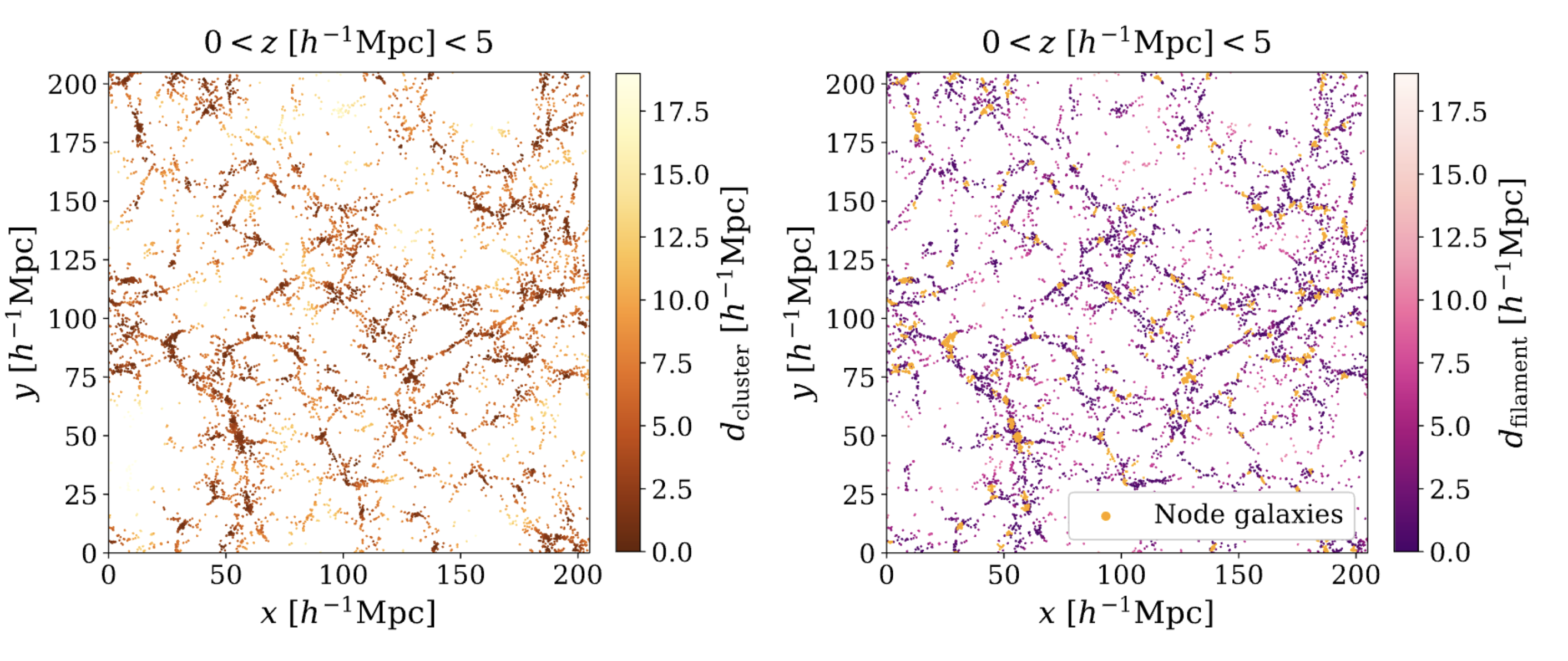
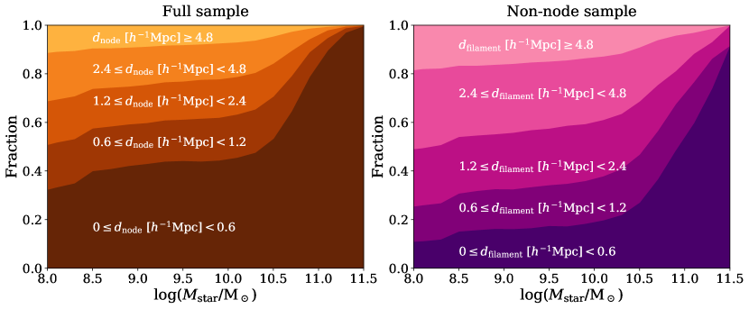
We quantify the cosmic web environment of galaxies in terms of their proximity to nearby dense structures, namely, the distance to the nearest node, , and the nearest filament, . We investigate the effects of nodes and filaments separately. Galaxies that are close to nodes are mainly affected by the node environment and are not as sensitive to the filaments around them, and in our analyses of , we exclude galaxies with . We refer to this sample as the non-node sample, in contrast to the full sample, which includes all galaxies with stellar masses greater than . In Figure 1, we illustrate these distances with a scatter plot of galaxies in a thin slice of the simulation box. We observe that most galaxies are distributed around nodes and along filaments, forming a web-like structure, as expected. In Figure 2, we show the fractions of galaxies with different distances to nodes and filaments, as functions of galaxy stellar mass. It is clear from the figure that more massive, brighter galaxies tend to inhabit node and filament environments. These proxies do not capture all the information from the cosmic web environment, and we will discuss other possibilities in Section 7.
2.3 Statistics
The connection between galaxies and haloes, together with the halo distribution, determines the spatial distribution of galaxies, and we measure galaxy clustering through summary statistics. We select two distinct statistics, the projected two-point correlation function and the counts-in-cylinders statistic , both of which are based on finding pairs of galaxies. We use the real-space positions of galaxies from the simulation, disregarding peculiar velocities. To make it easier to compare our results with those from observations, which will be explored in our future work, we still use projected statistics, which are less affected by redshift space uncertainties. We take the -axis as the line-of-sight direction for our measurements. We use the halotools package (Hearin et al., 2017) to make our measurements.
Two-point correlation functions encode the majority of information in near-Gaussian fields and are used as standard statistics in the literature. We measure the projected two-point correlation function,
| (1) |
where is the excess probability of finding galaxy pairs with projected and line-of-sight separations and , respectively. We choose , and compute in 10 logarithmically spaced radial bins between and .
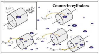
In Wang et al. (2019); Wang et al. (2022), we have demonstrated that the counts-in-cylinders statistics are an informative complement to the two-point statistics, because they encode higher-order information of the galaxy field. We measure the counts-in-cylinders statistic for a sample of galaxies by constructing cylinders of radius and half-length along the line of sight, centring them on each galaxy in the sample. We then count the number of companion galaxies in the sample that fall into each cylinder and use the distribution of this companion count as our summary statistic of the galaxy spatial distribution (illustrated in Figure 3). In real space, we use the same and of to probe sufficiently large scales in the spatial distribution of galaxies, and denote the count statistics with this cylinder size as . We have tested that different cylinder sizes do not affect our qualitative results (see Appendix B).
2.4 Catalogue shuffling
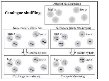
We measure the strength of the SGB with the shuffling technique, first proposed by Croton et al. (2007). Here, we present a detailed description of the shuffling method, which is also illustrated in Figure 4.
2.4.1 Mass shuffling
The SGB is the dependence of galaxy occupation on some secondary halo property (denoted as in Figure 4), which is either internal or environmental. This effect can be detected in galaxy clustering through its combination with the underlying halo clustering. To isolate the SGB, galaxies are randomly shuffled among haloes of the same mass, while preserving the phase-space distribution of satellite galaxies with respect to the central galaxy. This erases any dependence of galaxy occupation on halo properties other than mass. Comparing the shuffled and original clustering provides a quantification of the SGB. If there is no SGB present, the shuffling has no impact on the measured galaxy clustering. However, if there is SGB in the sample, the shuffling alters the galaxy clustering. In practise, galaxies are shuffled among haloes in narrow mass bins of 0.1 dex, over which the scatter introduced by the mass dependence is typically small.
2.4.2 Double shuffling
It is possible to further investigate the origins of the SGB with the double shuffling technique. This technique fixes the halo mass and a secondary halo property when reassigning galaxies among haloes. This eliminates any dependence of galaxy occupation on halo properties other than mass and the fixed secondary halo property. By comparing the mass shuffles, the double shuffles, and the original galaxy distribution, it is possible to determine the portion of the SGB that can be attributed to the secondary halo property, such as or , and the portion that cannot, thus indicating its relative importance in determining galaxy occupation.
2.5 Secondary galaxy bias strength
2.5.1 Ratio measurement
We measure the strength of the secondary galaxy bias (SGB) by comparing the statistics of the original and shuffled galaxy distributions, , where is the data vector. The deviation of these ratios from 1 can be used to detect the SGB, as the difference reflects the effect of the SGB on the statistics. For instance, ratios greater than 1 indicate that the SGB present in the original sample increases the value of the statistics, and vice versa. When and are measured from the original sample and mass shuffle, respectively, reveals the full extent of SGB from all sources; when and are measured from the double shuffle and the mass shuffle, respectively, indicates the SGB that can be attributed to the second halo property.
2.5.2 Uncertainty estimation
We provide an estimate of the statistical significance of our SGB signal by computing jackknife uncertainties of the ratios, as was done in Hadzhiyska et al. (2021). We divide the original simulation box and the shuffled simulation box into cuboid cells, each of size . The long axis of each cuboid is the same as the length of the simulation box and is assumed to lie along the line of sight. We calculate the data vector for the jackknife subsamples, excluding one cuboid at a time. The jackknifed ratios are calculated between pairs of jackknife subsamples that exclude the same cuboid, so that the ratios are only dependent on the changes in the galaxy occupation of haloes, not differences in host haloes themselves. We use the jackknife errors from these ratios to represent the uncertainty.
3 Measured Halo Occupation Distribution
The Halo Occupation Distribution (HOD) (e.g., Berlind & Weinberg, 2002; Kravtsov et al., 2004; Zheng et al., 2007) is a commonly used technique for modelling the relationship between galaxies and haloes. In its simplest form, the HOD assumes that the number of galaxies in a halo is determined solely by the halo mass. Secondary galaxy bias, however, implies a violation of this assumption. The HOD depends on the selection of the galaxy sample, as galaxies of different properties inhabit haloes in different ways. In this section, we will look at the HODs measured from the galaxy samples in IllustrisTNG and investigate whether and how they vary depending on the environment.
3.1 HODs of the entire samples
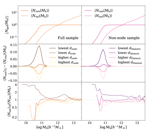
The HODs of central and satellite galaxies are usually modelled separately since dark matter haloes acquire them in distinct ways. In the top row of Figure 5, we display the central and satellite occupation as a function of halo mass, for both the full sample and the non-node sample. These are calculated from the ratio of galaxy number to halo number within each narrow halo mass bin, in a nonparametric form. The measured HODs are in agreement with expectations. Each halo can have either 0 or 1 central galaxy, but any number of satellite galaxies, and more massive haloes host more galaxies. The occupation for the non-node sample is limited to lower halo masses, since the most massive haloes and their galaxies are excluded.
3.2 Environmental dependence of the HOD
If the properties of galaxies depend not only on the mass of the halo, but also on a secondary halo property, (in this case, or ), haloes of the same mass with different values of will have different numbers of galaxies in a given sample. We divide the haloes in each narrow mass bin into four quartiles of (), and by comparing the HODs of the quartiles, the SGB associated with () can be determined.
We compare the occupation of the central galaxy for each quartile with respect to the entire sample in the middle row of Figure 5. We find that haloes closer to dense structures are more likely to host a central galaxy, with the preference being stronger for the full sample with nodes. The mean central number transitions from 0 at low halo masses to 1 at high halo masses, and the difference between quartiles is most prominent at masses slightly below . Furthermore, the dependence on node (filament) proximity is stronger at lower (), indicating that nodes and filaments mostly affect their immediate surroundings, and environments become less distinct from each other when they are far from these dense structures.
In the bottom row of Figure 5, we compare the mean satellite occupation of each quartile to that of the entire sample, , as a function of the halo mass, . The satellite statistics are noisy due to the low number densities of massive objects at the high mass end and the incomplete halo sample at the low mass end, caused by the finite-mass resolution of the simulation. Nevertheless, we still observe a trend similar to the central occupation, where haloes closer to nodes or filaments tend to host more satellite haloes, with the dependence weakening as the distance increases. This measurement suggests that the effects of nodes and filaments on satellite occupation are comparable.
In conclusion, we have demonstrated that there is a greater presence of node-related SGB than filament-related SGB in the central galaxy component of the TNG galaxy sample. Nevertheless, this method is restricted to individual secondary halo properties and cannot measure the total SGB from all sources. To address this, we will use the shuffling technique to determine the relative contribution of the environment-related SGB to the total SGB in the following sections.
4 Environment as Secondary Halo Property
We seek to answer two questions in this section: (i) what is the total amount of secondary galaxy bias (SGB) present in the IllustrisTNG galaxy sample, and (ii) how much of the total SGB can be attributed to the environmental properties, as quantified by the distances to nodes and filaments, and . To answer the first question, we compare and measurements between the original galaxy sample and the mass shuffled sample. To answer the second question, we compare measurements from the sample shuffled by both halo mass and the environment property, or , and the sample shuffled by halo mass alone.
4.1 Original measurements
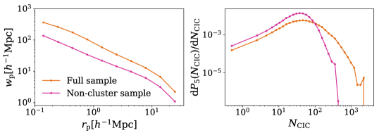
We first measure the statistics of the original galaxy sample from TNG300-1. In Figure 6, we show the measurements for both the full and non-node samples, with in the left panel and in the right panel. The two-point clustering is significantly reduced when node galaxies are excluded, and the fraction of groups with higher companion counts also decreases, resulting in a higher probability of having fewer companion galaxies in a cylinder, which is in line with our expectation, as node galaxies are a major contributor to the abundance of pairs and neighbours.
4.2 Secondary galaxy bias signal
We now repeat the measurements for different galaxy catalogues and compare the results between the original and shuffled samples. We make four sets of comparisons:
-
1.
The original full sample versus the full sample shuffled by mass;
-
2.
The full sample shuffled by mass and versus the full sample shuffled by mass;
-
3.
The original non-node sample versus the non-node sample shuffled by mass;
-
4.
The non-node sample shuffled by mass and versus the non-node sample shuffled by mass.
For the full sample, (i) evaluates the total SGB and (ii) evaluates the SGB that can be attributed to . For the non-node sample, (iii) evaluates the total SGB, and (iv) assesses the SGB that can be attributed to .
The results are shown in terms of the ratio between the statistics taken from the samples we are comparing. As we have discussed in Section 2.5, any difference from unity in the ratio can be seen as a sign of SGB in the sample, and the errors are determined from jackknife subsamples of the simulation box, providing an estimate of the statistical importance of the signal. Although the results here are based on one random shuffle of each type, we have tested that our results are consistent regardless of the random seed used in the shuffling process.
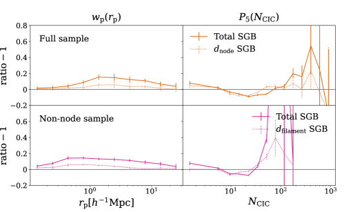
4.2.1 Full sample and effect
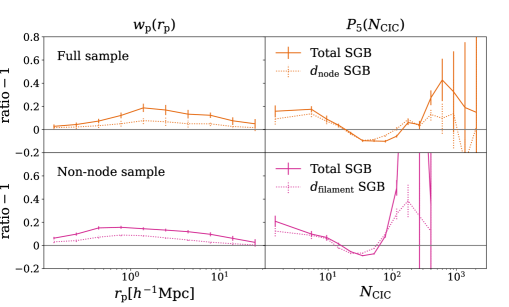
We first examine the SGB in the full sample, along with the contribution of . In the top row of Figure 7, we show the results of comparisons (i) and (ii), which indicate the strength of the total SGB present in the full sample. The solid curves with error bars represent comparison (i), the total SGB. We observe considerable SGB in the sample, as indicated by both and . The results demonstrate that SGB increases clustering in the range of scales that we investigate. The most prominent effect is seen at intermediate scales, since the shuffling process preserves the 1-halo term in the clustering, diminishing the difference at small scales, while the underlying secondary halo bias weakens at large scales.
The results show that SGB increases the likelihood of having a large and a small number of companion galaxies, while reducing the proportion of intermediate companion counts. This suggests that the overall effect of SGB is that the more clustered haloes tend to host more galaxies, adding to the large groups of galaxies in the distribution. At the same time, the less clustered haloes host fewer galaxies, resulting in more empty space in the galaxy distribution, which is reflected in the increased probability of low .
The dotted lines with error bars represent the SGB associated with . The comparison between the dotted and solid lines shows that has an effect on galaxy occupation in the same way as the total effect, namely, haloes with lower values of (which are closer to their neighbouring nodes) tend to host more galaxies at the same mass. This is in agreement with the results from Section 3. Although contributes significantly to the total SGB, it is not the only factor. It is not possible to determine the exact amount of contribution from due to scale dependences and the fact that the ratios do not translate directly to a physical fraction.
4.2.2 Non-node sample and effect
We investigate the SGB in the non-node sample, from which node galaxies are excluded, and the contribution from . The bottom row of Figure 7 displays the results. The solid curves with error bars represent comparison (iii), the total SGB, and the dotted curves correspond to comparison (iv), the -related SGB. The signals we detect are similar to those in Section 4.2.1, with enhanced on all scales and increased for small and large companion counts. This implies that even when node galaxies are excluded, haloes that are more clustered tend to host more galaxies. For in particular, more galaxies are found in haloes closer to the filaments, which is consistent with Section 3. The effect of can explain a significant part of the total secondary bias, but not all of it.
The discrepancies between the full sample and the non-node sample are evident. The uncertainties in the ratios are lower for the latter, suggesting that the effect of SGB is less reliant on the environment when nodes are excluded, implying that in the extreme environment of nodes, galaxy occupation has more varied behaviour. The peak of the difference in is on a slightly smaller scale than for the full sample, which is likely due to the smaller radii of haloes farther away from the nodes, and thus the earlier emergence of the 2-halo term. The effect of SGB on the small scale is reduced by the exclusion of node regions, which is likely the cause of the small discontinuity at a few . The measurements are cut off at a smaller (around ) for the non-node sample, due to the reduced group sizes without the node galaxies.
5 Dependence of Secondary Galaxy Bias on Environment
In the preceding section, we have studied the relative contribution of environmental measures as secondary halo properties to the total SGB in a galaxy sample. In this section, we explore the role of the cosmic web environment in the SGB from a different angle: whether galaxy samples with similar halo mass distributions but different environments display different levels of SGB. It is well known that both the secondary halo bias and the secondary galaxy bias are sensitive to halo mass (e.g., Wechsler et al., 2006; Wang et al., 2022). This, combined with the fact that halo masses are strongly correlated with the environment, presents a challenge for our analysis. Therefore, when comparing the SGB in different cosmic web environments, we need to separate the effect of or from the effect of the halo mass. To accomplish this, we divide the galaxy sample at the 50th percentile of the host or within each narrow bin of host halo masses, instead of percentiles in the entire sample. This approach ensures that the split subsamples have similar distributions of halo masses and prevents the halo mass dependence of SGB from masquerading as a dependence on or .
5.1 Secondary galaxy bias at different
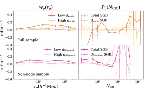
We investigate the dependence of SGB on the node environment by comparing the SGB signals in the two galaxy subsamples with low and high . The upper row of Figure 8 shows our measurements of the SGB effect of both statistics. The two subsamples with low and high are represented by different colours, as labelled in the top left panel. The solid curves and the dotted curves correspond to the total SGB and the -related SGB, respectively, as labelled in the top right panel, similar to Figure 7. We can see that the SGB signal is stronger in the high subsample than in the low subsample.
We find that for both subsamples, the total SGB increases the two-point clustering in the range of scales we investigate, and shifts companion counts in cylinders towards more extreme values111The only exception is in the lowest bin for the subsample closer to nodes, where the effect of the SGB reduces the probability, suggesting that the SGB in dense environments disfavours extreme isolation of galaxies., similar to the results from the entire sample. This can be interpreted as a positive correlation between halo clustering and galaxy occupation. In other words, in both subsamples, the haloes that are more strongly clustered also contain more galaxies.
By comparing the two subsamples, it is evident that the total SGB is significantly stronger at lower . The contrast in between the two subsamples is most noticeable at small scales, where the low subsample shows a positive signal, while the high curve is consistent with zero. This can be explained by the shuffling procedure, which preserves the 1-halo term and the larger separations between haloes in environments farther away from nodes, resulting in the 2-halo term appearing at larger scales. For , there is an overall decrease in counts in the high subsample compared to the low subsample, due to the lower number density of galaxies away from nodes, as well as the weakening of the SGB signal.
We now investigate the -related SGB, which is represented by the dotted lines. In the low subsample, there is a weak -related SGB signal, while the high subsample shows little evidence of -related SGB. This is in agreement with our findings in Section 3, which suggest that the HODs of samples further away from the nodes are less distinct from each other. Additionally, for both subsamples, the proportion of -related SGB to the total SGB in the subsamples is lower than in the entire sample, indicating that the dependence of galaxy occupation on is largely explained by the coarse division of galaxies into low and high subsamples. This also shows that the signal of and -related in Figure 7 can be largely ascribed to galaxy pairs across different environments.
5.2 Secondary galaxy bias at different
We investigate the dependence of the SGB on in the non-node sample. The bottom row of Figure 8 displays the results. The -related SGB effect is similar to the effect discussed in Section 5.1, with the total SGB being stronger at lower than higher , although the difference is not as pronounced as in the case. The statistic reveals a weak signal of -related SGB in the low subsample, while hardly shows a signal. In contrast, neither statistic detects a strong -related SGB in the high subsample.
In summary, regardless of whether the sample is divided into low or high , it is evident that more clustered haloes contain more galaxies. However, the preference is more pronounced in the low subsample. Furthermore, the amount of -related SGB is significantly reduced in both subsamples after the splitting, implying that the number of galaxies is mainly determined by the general type of environment in relation to nearby filaments, rather than by minor variations.
6 Discussion
In this study, we investigated the impact of the cosmic web on the SGB by examining its effect on galaxy clustering measurements. We will now discuss the implications of our findings, as well as some of the restrictions of this study.
In Section 3, we compared the halo occupation distribution in different environments. We found that at fixed halo mass, haloes close to nodes and filaments host more galaxies. Rather than parametrised fits, this halo occupation distribution measurement is a direct measurement of the SGB attributable to the distance between the host halo and dense cosmic web structures. Previous studies, for example, Croft et al. (2012); Zehavi et al. (2018) and Bose et al. (2019), have also found that the halo occupation distribution is higher for haloes in environments with higher intermediate-scale overdensities. Their findings are broadly consistent with ours, although we use different proxies for the environment compared to the overdensity criteria used in these works: haloes located near nodes and filaments tend to have surrounding overdensities higher than those of other haloes.
Our research is one of the first to investigate the role of the cosmic web in the secondary galaxy bias effect. Hadzhiyska et al. (2020) used the IllustrisTNG simulation to explore the effect of local environment by employing a proxy of the local mass density and found that galaxies in similar environments tend to cluster together, which is in line with our results that the coarse division of the galaxy sample by types largely explains the environment-related secondary galaxy bias. Xu et al. (2021) studied the relative contribution of cosmic web environment types to the total secondary galaxy bias using the Millenium simulation and concluded that the environment type measured on scales of constitutes a considerable portion of the total secondary bias signature. This is in agreement with our findings from Section 4, although we use different indicators of the environment. As we were completing this manuscript, we became aware of an independent analysis by Montero-Dorta & Rodriguez (2023), who also used distances from cosmic web structures to describe the environment. They found that at fixed halo mass, objects closer to dense structures cluster more strongly, which accounts for a significant portion of the dependence of galaxy clustering on halo formation time, also in qualitatively agreement with our findings.
In Section 5, we present a novel element in the relation between the cosmic web and the SGB: to what extent haloes in different cosmic web environments exhibit different SGB behaviours. We find that haloes close to nodes and filaments are subject to stronger SGB. We argue that this is an important component of the cosmic web effect, as it sheds light on fundamental differences in the physics of galaxy formation and evolution between different environments.
In this work, we have focused on the connection between the cosmic web and the SGB, in other words, the response of the galaxy–halo connection to the environment. We note that there is a relatively larger volume of work on the influence of the environment on the halo bias. For example, Pujol et al. (2017) and Shi & Sheth (2018) claimed that halo clustering is completely determined by the local environment. Paranjape et al. (2018) found that haloes in isotropic and anisotropic environments show different halo assembly biases, Ramakrishnan et al. (2019) showed that halo clustering depends on internal halo properties only through tidal anisotropy, and Mansfield & Kravtsov (2020) proposed the tidal and gravitational effects of the surrounding large-scale structure as main causes of low-mass halo assembly bias. These results indicate that the environments of haloes play a physically fundamental role in determining the halo clustering, which is connected to the traditionally studied halo assembly bias.
We discuss how the cosmic web effect on SGB connects to some of the more commonly studied secondary halo properties. In particular, studies have extensively examined the secondary galaxy bias associated with halo concentration, formation time, spin, etc. Each of these halo properties affects the galaxy occupation beyond halo mass (see, e.g., Xu et al., 2021, for a systematic study). Haloes in different cosmic web environments have systematically different assembly histories that are reflected in their secondary properties. For example, haloes that frequently merge are likely to have later formation times and lower concentrations. It has also been shown that low-concentration haloes tend to host more satellite galaxies (e.g., Wang et al., 2022), consistent with late formers having more frequent recent mergers. Although the cosmic web and traditional secondary properties are connected, we argue that the cosmic web environment provides a more fundamental view of the factors that affect galaxy formation and evolution.
The cosmic web descriptors are linked to the causal elements of the assembly histories. For instance, node haloes often experience frequent mergers, which are supplied by the filaments that connect them. Moreover, haloes in different cosmic web environments experience different tidal fields. At the most extreme end of the environmental range, massive node haloes have a major influence on their tidal environment and affect nearby haloes through anisotropic tidal forces. These cosmic web descriptors include distances to dense structures, which are used in this work, and measurements of the surrounding density, which are used in other works. By using cosmic web descriptors as a secondary feature, we can investigate their role in the formation of galaxies.
In this work, we study the secondary galaxy bias, which explicitly excludes the effect of halo mass on galaxy properties, and we underline the importance of disentangling the halo mass effect from the contribution of any secondary factor to galaxy formation and evolution. The success of various galaxy–halo connection models (see Wechsler & Tinker, 2018, and references therein) has demonstrated that halo mass (or some mass-like measure) is the predominant determinant of the properties of its galaxies. As halo mass is known to correlate with almost all other halo properties (e.g., Wechsler et al., 2002; Macciò et al., 2007; Knebe & Power, 2008), any apparent sensitivity of galaxy properties to secondary halo properties could, in fact, have a root in the halo mass dependence. It is crucial to always account for halo mass in the theoretical framework, and while it is more challenging to estimate halo masses in observational data, careful considerations of its effect should be made before drawing conclusions on physical factors that impact galaxy formation and evolution.
One might posit that any environmental dependence of galaxy occupation might be due to a halo mass dependence: we expect more massive haloes to prefer overdense regions of our Universe. However, our research has revealed that galaxies prefer to live near nodes and filaments, even when the halo mass is taken into consideration. This preference indicates that the cosmic web has a more complex effect on galaxy physics. These effects could be due to the different halo assembly histories, as well as surrounding tidal anisotropies, which we have discussed above. Galaxies in haloes with different assembly histories will form in different potential wells and have different merger histories, leading to different star formation histories, dynamical states and morphologies. On the other hand, the anisotropic tidal field may strip galaxies of their cold gas, or heat the gas reservoir, thus suppressing star formation as galaxies move through the cosmic web (e.g., Guo et al., 2021, 2023).
Our findings are based on the cosmic web structure identified by the DisPerSE cosmic web finder. Other algorithms, such as those discussed in summarised in Table 1 of Libeskind et al. (2018), may lead to different descriptions of the environment of individual objects. Nevertheless, the general behaviour of these algorithms is in agreement with each other, and we do not anticipate our primary conclusions to be altered by alternative cosmic web identification methods. It is worth noting that our quantification of the environment of haloes and galaxies, i.e., the distance to nearby dense structures, is not a comprehensive description of the environment information. For instance, this metric does not take into account the relative location of an object along a filament, nor does it differentiate between nodes or filaments with different densities and sizes. We do not consider cosmic sheets and voids in this work either. Therefore, we cannot definitively rule out the possibility that the secondary galaxy bias is completely rooted in the cosmic web environment.
Our analysis demonstrates the ability of to investigate the nuances of secondary galaxy bias, with a statistically significant measurement of environmental contributions to the SGB. As argued in Wang et al. (2022), while the two-point correlation function mainly concentrates on the densest parts of the galaxy distribution, the counts-in-cylinders statistic, , is sensitive to all but the most extreme underdensities, and measures higher-order statistics of the galaxy field. In forward modelling approaches, provides additional information on the two-point statistics, and in our shuffling procedure, the changes in also reveal a level of detail that contributes to our understanding of the underlying physics.
7 Conclusions
In this study, we explore a link between the cosmic web environment and the galaxy–halo connection. First, we treat the host halo proximity to nodes and filaments as a secondary halo property, and quantify its relative contribution to the total secondary galaxy bias. Second, we compare the behaviour of the secondary galaxy bias in different environments. Our findings are summarised as follows.
-
•
We identify dense structures in the cosmic web (nodes and filaments) in the TNG300-1 run of the IllustrisTNG simulation, using the DisPerSE algorithm. We use halo distances to these dense structures as an environmental measure. We illustrate general features of the cosmic web with these measures in Figure 1 and Figure 2.
-
•
We directly measure the halo occupation distribution for our galaxy sample with stellar masses above , and find that haloes closer to nodes or filaments tend to host more galaxies at fixed halo mass (Figure 5).
-
•
We compare summary statistics of shuffled and original galaxy samples to quantify the total secondary galaxy bias and the component that can be attributed to our environmental measures (see Figure 4 for a schematic illustration). In addition to the projected two-point correlation function, , we include a novel perspective with the counts-in-cylinders statistics, (see Figure 3 for the definition of ). Figure 6 provides examples of both statistics.
-
•
In our chosen summary statistics, we confirm that the secondary galaxy bias causes an enhancement in the two-point clustering, and we expose a nuanced effect with the counts-in-cylinders statistics, which manifests as a redistribution of galaxies from intermediate sized companion groups into groups with either very large or very small numbers of galaxies (solid curves in Figure 7). We conclude that the total effect of secondary galaxy bias is for galaxies to preferentially reside in more strongly clustered haloes at similar halo masses.
-
•
We find that the host halo distance to nodes or filaments can account for a significant portion of the total secondary galaxy bias, but not the entire effect (see comparison between solid and dotted curves in Figure 7).
-
•
We find that the total effect of secondary galaxy bias is relatively stronger for subsamples that are closer to nodes or filaments (see comparison between different coloured solid curves in Figure 8). Within each subsample, the environmental component of SGB weakens (see reduced deviation of the ratio from unity in dotted curves in Figure 8). This trend indicates that while host haloes closer or further from dense cosmic web structures have different galaxy occupations, the finer details of the environment beyond this qualitative classification is less important in the galaxy–halo connection. We stress the importance of comparing galaxy samples with similar host halo mass distributions to isolate the effects of environment.
This work lays out a framework to comprehensively investigate the role of the cosmic web in the galaxy–halo connection, and constitutes a critical step towards understanding the role of the environment in galaxy formation and evolution. In the future, we will explore alternative descriptions of the cosmic web, and extend the analysis to observational data.
Acknowledgements
We thank Johannes Lange, Risa Wechsler, Andrew Zentner and Qiong Zhang for useful discussions.
KW acknowledges support from the Leinweber Postdoctoral Research Fellowship at the University of Michigan. CA acknowledges support from the Leinweber Center for Theoretical Physics and DOE grant DE- SC009193. HG is supported by the National SKA Program of China (grant No. 2020SKA0110100), National Natural Science Foundation of China (Nos. 11922305, 11833005), the CAS Project for Young Scientists in Basic Research (No. YSBR-092) and the science research grants from the China Manned Space Project with NOs. CMS-CSST-2021-A02. PW is sponsored by Shanghai Pujiang Program(No. 22PJ1415100).
This research made use of Python, along with many community-developed or maintained software packages, including IPython (Pérez & Granger, 2007), Jupyter (jupyter.org), Matplotlib (Hunter, 2007), NumPy (van der Walt et al., 2011), SciPy (Jones et al., 2001), and Astropy (Astropy Collaboration et al., 2013). This research made use of NASA’s Astrophysics Data System for bibliographic information.
Data Availability
The simulation underlying this article were accessed from publicly available sources: https://www.tng-project.org/data/. The catalogues including the cosmic web information will be shared on reasonable request to the corresponding authors. The additional derived data are available in the article.
References
- Alam et al. (2019) Alam S., Zu Y., Peacock J. A., Mandelbaum R., 2019, MNRAS, 483, 4501
- Aragón-Calvo et al. (2010) Aragón-Calvo M. A., van de Weygaert R., Jones B. J. T., 2010, MNRAS, 408, 2163
- Aragon Calvo et al. (2019) Aragon Calvo M. A., Neyrinck M. C., Silk J., 2019, The Open Journal of Astrophysics, 2, 7
- Artale et al. (2018) Artale M. C., Zehavi I., Contreras S., Norberg P., 2018, MNRAS, 480, 3978
- Astropy Collaboration et al. (2013) Astropy Collaboration et al., 2013, A&A, 558, A33
- Azzaro et al. (2007) Azzaro M., Patiri S. G., Prada F., Zentner A. R., 2007, MNRAS, 376, L43
- Berlind & Weinberg (2002) Berlind A. A., Weinberg D. H., 2002, ApJ, 575, 587
- Blanton et al. (2005) Blanton M. R., Eisenstein D., Hogg D. W., Schlegel D. J., Brinkmann J., 2005, ApJ, 629, 143
- Blumenthal et al. (1984) Blumenthal G. R., Faber S. M., Primack J. R., Rees M. J., 1984, Nature, 311, 517
- Bond et al. (1996) Bond J. R., Kofman L., Pogosyan D., 1996, Nature, 380, 603
- Bond et al. (2010) Bond N. A., Strauss M. A., Cen R., 2010, MNRAS, 406, 1609
- Borzyszkowski et al. (2017) Borzyszkowski M., Porciani C., Romano-Díaz E., Garaldi E., 2017, MNRAS, 469, 594
- Bose et al. (2019) Bose S., Eisenstein D. J., Hernquist L., Pillepich A., Nelson D., Marinacci F., Springel V., Vogelsberger M., 2019, MNRAS, 490, 5693
- Cautun et al. (2014) Cautun M., van de Weygaert R., Jones B. J. T., Frenk C. S., 2014, MNRAS, 441, 2923
- Cooper et al. (2010) Cooper M. C., Gallazzi A., Newman J. A., Yan R., 2010, MNRAS, 402, 1942
- Croft et al. (2012) Croft R. A. C., di Matteo T., Khandai N., Springel V., Jana A., Gardner J. P., 2012, MNRAS, 425, 2766
- Croton et al. (2007) Croton D. J., Gao L., White S. D. M., 2007, MNRAS, 374, 1303
- Davis et al. (1985) Davis M., Efstathiou G., Frenk C. S., White S. D. M., 1985, ApJ, 292, 371
- Dressler (1980) Dressler A., 1980, ApJ, 236, 351
- Eardley et al. (2015) Eardley E., et al., 2015, MNRAS, 448, 3665
- Efstathiou & Jones (1979) Efstathiou G., Jones B. J. T., 1979, MNRAS, 186, 133
- Faltenbacher et al. (2009) Faltenbacher A., Li C., White S. D. M., Jing Y.-P., Shu-DeMao Wang J., 2009, Research in Astronomy and Astrophysics, 9, 41
- Forero-Romero et al. (2014) Forero-Romero J. E., Contreras S., Padilla N., 2014, MNRAS, 443, 1090
- Forman (2002) Forman R., 2002, Séminaire Lotharingien de Combinatoire [electronic only], 48, B48c
- Galárraga-Espinosa et al. (2020) Galárraga-Espinosa D., Aghanim N., Langer M., Gouin C., Malavasi N., 2020, A&A, 641, A173
- Gao & White (2007) Gao L., White S. D. M., 2007, MNRAS, 377, L5
- Gao et al. (2005) Gao L., Springel V., White S. D. M., 2005, MNRAS, 363, L66
- González & Padilla (2009) González R. E., Padilla N. D., 2009, MNRAS, 397, 1498
- Gottlöber et al. (2001) Gottlöber S., Klypin A., Kravtsov A. V., 2001, ApJ, 546, 223
- Guo et al. (2015) Guo H., et al., 2015, MNRAS, 453, 4368
- Guo et al. (2021) Guo H., Jones M. G., Wang J., Lin L., 2021, ApJ, 918, 53
- Guo et al. (2023) Guo H., Wang J., Jones M. G., Behroozi P., 2023, arXiv e-prints, p. arXiv:2307.07078
- Hadzhiyska et al. (2020) Hadzhiyska B., Bose S., Eisenstein D., Hernquist L., Spergel D. N., 2020, MNRAS, 493, 5506
- Hadzhiyska et al. (2021) Hadzhiyska B., Liu S., Somerville R. S., Gabrielpillai A., Bose S., Eisenstein D., Hernquist L., 2021, MNRAS, 508, 698
- Hahn et al. (2007a) Hahn O., Porciani C., Carollo C. M., Dekel A., 2007a, MNRAS, 375, 489
- Hahn et al. (2007b) Hahn O., Carollo C. M., Porciani C., Dekel A., 2007b, MNRAS, 381, 41
- Hahn et al. (2009) Hahn O., Porciani C., Dekel A., Carollo C. M., 2009, MNRAS, 398, 1742
- Hahn et al. (2010) Hahn O., Teyssier R., Carollo C. M., 2010, MNRAS, 405, 274
- Hearin et al. (2016) Hearin A. P., Zentner A. R., van den Bosch F. C., Campbell D., Tollerud E., 2016, MNRAS, 460, 2552
- Hearin et al. (2017) Hearin A. P., et al., 2017, AJ, 154, 190
- Hunter (2007) Hunter J. D., 2007, Computing in Science Engineering, 9, 90
- Jõeveer et al. (1978) Jõeveer M., Einasto J., Tago E., 1978, MNRAS, 185, 357
- Jing et al. (2007) Jing Y. P., Suto Y., Mo H. J., 2007, ApJ, 657, 664
- Jones et al. (2001) Jones E., Oliphant T., Peterson P., et al., 2001, SciPy: Open source scientific tools for Python, http://www.scipy.org/
- Kasun & Evrard (2005) Kasun S. F., Evrard A. E., 2005, ApJ, 629, 781
- Knebe & Power (2008) Knebe A., Power C., 2008, ApJ, 678, 621
- Kodama et al. (2001) Kodama T., Smail I., Nakata F., Okamura S., Bower R. G., 2001, ApJ, 562, L9
- Kraljic et al. (2018) Kraljic K., et al., 2018, MNRAS, 474, 547
- Kravtsov et al. (2004) Kravtsov A. V., Berlind A. A., Wechsler R. H., Klypin A. A., Gottlöber S., Allgood B., Primack J. R., 2004, ApJ, 609, 35
- Lange et al. (2019) Lange J. U., van den Bosch F. C., Zentner A. R., Wang K., Villarreal A. S., 2019, MNRAS, 482, 4824
- Lehmann et al. (2017) Lehmann B. V., Mao Y.-Y., Becker M. R., Skillman S. W., Wechsler R. H., 2017, ApJ, 834, 37
- Li et al. (2008) Li Y., Mo H. J., Gao L., 2008, MNRAS, 389, 1419
- Libeskind et al. (2018) Libeskind N. I., et al., 2018, MNRAS, 473, 1195
- Macciò et al. (2007) Macciò A. V., Dutton A. A., van den Bosch F. C., Moore B., Potter D., Stadel J., 2007, MNRAS, 378, 55
- Mansfield & Kravtsov (2020) Mansfield P., Kravtsov A. V., 2020, MNRAS, 493, 4763
- Mao et al. (2018) Mao Y.-Y., Zentner A. R., Wechsler R. H., 2018, MNRAS, 474, 5143
- Marinacci et al. (2018) Marinacci F., et al., 2018, MNRAS, 480, 5113
- McCarthy et al. (2019) McCarthy K. S., Zheng Z., Guo H., 2019, MNRAS, 487, 2424
- Mo et al. (2010) Mo H., van den Bosch F. C., White S., 2010, Galaxy Formation and Evolution. Cambridge University Press
- Montero-Dorta & Rodriguez (2023) Montero-Dorta A. D., Rodriguez F., 2023, arXiv e-prints, p. arXiv:2309.12401
- Musso et al. (2018) Musso M., Cadiou C., Pichon C., Codis S., Kraljic K., Dubois Y., 2018, MNRAS, 476, 4877
- Naiman et al. (2018) Naiman J. P., et al., 2018, MNRAS, 477, 1206
- Navarro et al. (2004) Navarro J. F., Abadi M. G., Steinmetz M., 2004, ApJ, 613, L41
- Nelson et al. (2018) Nelson D., et al., 2018, MNRAS, 475, 624
- Nelson et al. (2019) Nelson D., et al., 2019, Computational Astrophysics and Cosmology, 6, 2
- Paranjape et al. (2018) Paranjape A., Hahn O., Sheth R. K., 2018, MNRAS, 476, 3631
- Paz et al. (2008) Paz D. J., Stasyszyn F., Padilla N. D., 2008, MNRAS, 389, 1127
- Pérez & Granger (2007) Pérez F., Granger B. E., 2007, Computing in Science Engineering, 9, 21
- Pillepich et al. (2018) Pillepich A., et al., 2018, MNRAS, 475, 648
- Pimbblet et al. (2004) Pimbblet K. A., Drinkwater M. J., Hawkrigg M. C., 2004, MNRAS, 354, L61
- Planck Collaboration et al. (2016) Planck Collaboration et al., 2016, A&A, 594, A13
- Pujol et al. (2017) Pujol A., Hoffmann K., Jiménez N., Gaztañaga E., 2017, A&A, 598, A103
- Ramakrishnan et al. (2019) Ramakrishnan S., Paranjape A., Hahn O., Sheth R. K., 2019, MNRAS, 489, 2977
- Sales & Lambas (2004) Sales L., Lambas D. G., 2004, MNRAS, 348, 1236
- Sheth & Tormen (2004) Sheth R. K., Tormen G., 2004, MNRAS, 350, 1385
- Shi & Sheth (2018) Shi J., Sheth R. K., 2018, MNRAS, 473, 2486
- Sobral et al. (2011) Sobral D., Best P. N., Smail I., Geach J. E., Cirasuolo M., Garn T., Dalton G. B., 2011, MNRAS, 411, 675
- Sousbie (2011) Sousbie T., 2011, MNRAS, 414, 350
- Sousbie et al. (2011) Sousbie T., Pichon C., Kawahara H., 2011, MNRAS, 414, 384
- Springel (2010) Springel V., 2010, MNRAS, 401, 791
- Springel et al. (2001) Springel V., White S. D. M., Tormen G., Kauffmann G., 2001, MNRAS, 328, 726
- Springel et al. (2018) Springel V., et al., 2018, MNRAS, 475, 676
- Tempel & Libeskind (2013) Tempel E., Libeskind N. I., 2013, ApJ, 775, L42
- Tempel et al. (2013) Tempel E., Stoica R. S., Saar E., 2013, MNRAS, 428, 1827
- Tojeiro et al. (2017) Tojeiro R., et al., 2017, MNRAS, 470, 3720
- Trowland et al. (2013) Trowland H. E., Lewis G. F., Bland-Hawthorn J., 2013, ApJ, 762, 72
- Vakili et al. (2016) Vakili M., et al., 2016, In Preparation
- Wang et al. (2011) Wang H., Mo H. J., Jing Y. P., Yang X., Wang Y., 2011, MNRAS, 413, 1973
- Wang et al. (2013) Wang L., Weinmann S. M., De Lucia G., Yang X., 2013, MNRAS, 433, 515
- Wang et al. (2019) Wang K., et al., 2019, MNRAS, 488, 3541
- Wang et al. (2022) Wang K., Mao Y.-Y., Zentner A. R., Guo H., Lange J. U., van den Bosch F. C., Mezini L., 2022, MNRAS, 516, 4003
- Wechsler & Tinker (2018) Wechsler R. H., Tinker J. L., 2018, ARA&A, 56, 435
- Wechsler et al. (2002) Wechsler R. H., Bullock J. S., Primack J. R., Kravtsov A. V., Dekel A., 2002, ApJ, 568, 52
- Wechsler et al. (2006) Wechsler R. H., Zentner A. R., Bullock J. S., Kravtsov A. V., Allgood B., 2006, ApJ, 652, 71
- White (1984) White S. D. M., 1984, ApJ, 286, 38
- White & Rees (1978) White S. D. M., Rees M. J., 1978, MNRAS, 183, 341
- Wu et al. (2008) Wu H., Rozo E., Wechsler R. H., 2008, ApJ, 688, 729
- Xu et al. (2021) Xu X., Zehavi I., Contreras S., 2021, MNRAS, 502, 3242
- Yang et al. (2017) Yang X., et al., 2017, ApJ, 848, 60
- Yuan et al. (2022) Yuan S., Hadzhiyska B., Bose S., Eisenstein D. J., 2022, MNRAS, 512, 5793
- Zehavi et al. (2011) Zehavi I., et al., 2011, ApJ, 736, 59
- Zehavi et al. (2018) Zehavi I., Contreras S., Padilla N., Smith N. J., Baugh C. M., Norberg P., 2018, ApJ, 853, 84
- Zentner et al. (2014) Zentner A. R., Hearin A. P., van den Bosch F. C., 2014, MNRAS, 443, 3044
- Zentner et al. (2019) Zentner A. R., Hearin A., van den Bosch F. C., Lange J. U., Villarreal A., 2019, MNRAS, 485, 1196
- Zhang et al. (2009) Zhang Y., Yang X., Faltenbacher A., Springel V., Lin W., Wang H., 2009, ApJ, 706, 747
- Zhang et al. (2013) Zhang Y., Yang X., Wang H., Wang L., Mo H. J., van den Bosch F. C., 2013, ApJ, 779, 160
- Zheng et al. (2007) Zheng Z., Coil A. L., Zehavi I., 2007, ApJ, 667, 760
- de Lapparent et al. (1986) de Lapparent V., Geller M. J., Huchra J. P., 1986, ApJ, 302, L1
- van der Walt et al. (2011) van der Walt S., Colbert S. C., Varoquaux G., 2011, Computing in Science Engineering, 13, 22
Appendix A Alternative Stellar Mass Samples
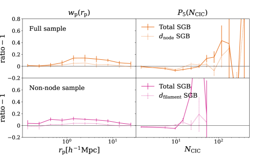
In this appendix, we repeat our analyses for alternative galaxy samples, with stellar mass thresholds of and , instead of in the main text. We limit our tests to these thresholds, because as can be seen in Figure 2, samples with higher stellar masses are predominantly found very close to nodes and filaments, and have less different environments. We show the results for these alternative samples in 1(a) and 1(b). Each figure is analogous to Figure 7, where the two columns show results from and respectively, and the two rows show results for the full and non-node samples respectively. The solid curves indicate the strength of the total SGB from all sources, and the dotted curves are specific to or -related SGB. We find that for the more massive galaxy samples, the same conclusions hold as for the sample. Namely, the effect of the total SGB is a preference of galaxies to populate haloes that are more strongly clustered; for and , galaxies prefer haloes closer to the overdense structures, which effect accounts for a significant fraction of the total SGB, but does not explain all of it. The only notable difference between the samples is that the signals in are shifted towards lower counts as the stellar mass threshold increases, because of the brighter samples have lower number densities and therefore fewer companions. Because of this shift, the increase of at low counts due to SGB disappears in the sample.
Appendix B Alternative Cylinder Sizes
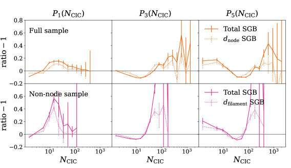
Our main results are based on measured with the cylinder radius and half-length of 5 . In this appendix, we test the robustness of our conclusions by measuring with alternative cylinder sizes. Our test results are shown in Figure B.1. Each column in this figure is analogous to the right column of Figure 7, but shows measurements with cylinder sizes of 1, 3, and 5 respectively, from left to right. As can be naively expected, with smaller cylinder sizes, probes the more immediate surroundings of galaxies, and has generally fewer companions. We observe an overall downscaling of with smaller cylinders compared to the 5 case. For example, in the middle column, the qualitative behaviour of with the cylinder size of 3 is similar to the 5 measurement at , and the signal in the left column is similar to the 5 measurement at . This is consistent with our main conclusions. The effect of the SGB places more galaxies in highly clustered haloes, and leaves the less clustered haloes underpopulated. With the large 5 cylinders, this increases the probability of having cylinders with both high in dense regions and low in underdense regions, as discussed in the main text. However, the haloes in underdense environments that host very few galaxies are not probed by the smaller cylinders, which eliminates the increase of low probabilities. The comparison between different cylinder sizes shows that we need to probe sufficiently large scales in order to fully observe the imprint of the SGB.