Non-standard quantum algebras and finite dimensional -symmetric systems
Abstract
In this work, -symmetric Hamiltonians defined on quantum algebras are presented. We study the spectrum of a family of non-Hermitian Hamiltonians written in terms of the generators of the non-standard Hopf algebra deformation of . By making use of a particular boson representation of the generators of , both the co-product and the commutation relations of the quantum algebra are shown to be invariant under the -transformation. In terms of these operators, we construct several finite dimensional -symmetry Hamiltonians, whose spectrum is analytically obtained for any arbitrary dimension. In particular, we show the appearance of Exceptional Points in the space of model parameters and we discuss the behaviour of the spectrum both in the exact -symmetry and the broken -symmetry dynamical phases. As an application, we show that this non-standard quantum algebra can be used to define an effective model Hamiltonian describing accurately the experimental spectra of three-electron hybrid qubits based on asymmetric double quantum dots. Remarkably enough, in this effective model, the deformation parameter has to be identified with the detuning parameter of the system.
-
September 26
Keywords: non-standard Hopf algebras, -symmetry, spectrum, exceptional points, effective Hamiltonians.
1 Introduction
Since the celebrated work of Bender and Boetcher [1], the study of mathematical properties [2, 3, 4, 5, 6, 7, 8] and physical applications [9, 10] of non-hermitian Hamiltonians has grown exponentially. Among non-hermitian operators, those obeying Parity-Time Reversal symmetry (-symmetry) have received particular attention, due to the rich structure that both its spectrum and dynamics [8] do present. A characteristic feature of these Hamiltonians is that its space of model parameters consists of two regions of well-defined structure: A region with real spectrum, where the eigenvectors of the Hamiltonian are also eigenvectors of the -symmetry operator (the so-called exact -symmetry phase) and another region where the spectrum includes complex pair conjugate eigenvalues (the broken -symmetry phase), where the eigenstates of the Hamiltonian are not eigenstates of the -symmetry operator. The boundary between these two regions is formed by the so-called Exceptional Points (EPs) [11, 12, 13]. At these latter values of the parameters of the model, two or more eigenvalues are degenerated and their eigenstates are coalescent. The consequence of the existence of EPs has been intensively analysed both theoretically [11, 10, 13] and experimentally [12, 10].
In this work, we investigate the features of the spectra of a family of -symmetry Hamiltonians defined on a non-standard Hopf algebra deformation of [14, 15, 16, 17, 18], whose finite-dimensional boson representations were constructed in [15, 16]. By suitably modifying these representations we will be able to establish a -invariant realisation of the Hopf algebra. Therefore, in terms of these operators, we will be able to construct a family of -symmetric Hamiltonians whose spectra will be analysed. Moreover, we shall show that this realisation of the quantum algebra is physically sound since it can be used to define effective Hamiltonians that reproduce the structure of the eigenvalues that have been recently obtained for Hamiltonian models describing realistic systems of semiconductor quantum dots.
The paper is organised as follows. In Section 2 we review the essentials of the non-standard quantum algebra and find a boson representation for which its Hopf algebra structure is fully invariant under -symmetry transformations. In Section 3, we construct two different families of Hamiltonians in terms of the -symmetric generators of . Afterwards, we study their spectra by introducing similarity transformations for them to obtain isospectral Hamiltonians, and we discuss the regions in the space of parameters showing -symmetry and broken -symmetry, as well as the associated sets of EPs. As an application of these non-hermitian Hamiltonians, in Section 4 we introduce a suitable choice of the Hamiltonian and its parameters that reproduces the spectra of a system of three electrons in an asymmetric two-dimensional double well, which has been recently implemented experimentally [19]. Conclusions and outlook are given in Section 5.
2 Formalism
In this section, after reviewing the essentials of the non-standard quantum Hopf algebra [14, 15, 16, 17, 18], we shall introduce a boson realisation of this algebra that is shown to be invariant under the -transformation. This will be the realisation used in the rest of the paper in order to define new non-hermitian and -symmetric Hamiltonian models.
2.1 Dyson’s boson representation of
Let us begin by summarising the properties of the Lie algebra (see, for instance, [20]) whose generators, , obey the well known commutation relations
| (1) |
We point out that -symmetric realisations of can be constructed in terms of boson operators, e.g.
| (2) |
where is the creation operator, the annihilation operator and a free real parameter which is directly related with the eigenvalue of the Casimir operator .
The realisation (2) is a modification of the Gelfan’d-Dyson (GD) one-boson realisation [21, 22]. It can be straightforwardly shown that (2) is invariant under the -transformation, since for . As a consequence, many Hamiltonian systems constructed in terms of the bosonic mapping (2) of the generators of will obey -symmetry.
As an instructive example, we shall study the properties of the spectrum of the linear Hamiltonian
| (3) |
It is straightforward to prove that for real , this Hamiltonian is invariant under a -transformation. Following [23, 24], in order to find the associated spectrum, we can introduce a similarity transformation such that . In the following Proposition, we state the characteristics of the spectrum of depending on the sign of .
Proposition 1. Let .
a) If and , then is hermitian for .
b) For , is a diagonal matrix with complex pair-conjugate eigenvalues.
Proof.
By using the relations presented in A, we have
In the bosonic realisation (2), is the only hermitian generator. Then, to find the isospectral hermitian operator associated with we need to cancel the terms including and . Because of that, we obtain the equations
whose solution is . In that case,
| (4) |
Thus, has real spectrum for and has complex pair-conjugate eigenvalues for . ∎
2.2 The non-standard quantum algebra
Many authors have considered different deformations of the algebra and have applied them in different contexts (see, for instance, [25, 26, 27, 28]). We recall that among all possible deformations of a given Lie algebra, a distinguished class is defined by the Hopf algebra deformations of the Universal Enveloping Algebra (UEA) of such Lie algebra. These deformed Hopf algebras are called Quantum Universal Enveloping Algebras (QUEA) or, in short, quantum algebras, and are defined as simultaneous and compatible deformations of both the commutation rules of the Lie algebra and the coproduct map that defines its tensor product representations [29, 30].
In the case of , we will deal with the so-called non-standard quantum deformation [15, 16] (the standard deformation is the Drinfel’d-Jimbo one [31, 32]). Its generators, named , where is a real deformation parameter, define the quantum algebra relations through the commutation rules
| (5) |
which are just a generalisation of (1), which is smoothly recovered in the limit.
Tensor product representations of the quantum algebra (5) are obtained through the so-called coproduct map
| (6) |
which defines an algebra homomorphism between and . As expected, the limit leads to the usual (undeformed) rule for the construction of tensor product representations.
We are interested in getting the non-standard deformed generalisation of the -symmetric GD realisation (2). Such a result can be obtained by starting from the boson representation obtained in [16, 15], together with the definition of the new set of operators, as
| (7) |
In such a way we obtain
| (8) | |||||
These operators can be straightforwardly shown to be -symmetric, and we stress that the transformation is essential in order to recover the symmetry of this boson representation of the deformed algebra.
The action of the operators on the eigenstates of the usual boson number operator , provides their lower-bounded representation, namely
| (9) |
As it was shown in [16], for values of the parameter , this representation becomes reducible and leads to the -symmetric finite-dimensional irreducible representations of dimension of the quantum algebra .
The commutation rules, coproduct (), counit (), and antipode () maps defining the full Hopf algebra structure of in terms of the -symmetric generators indeed have the same structure as those of (see B). Namely,
| (10) | |||||
| (11) | |||||
| (12) | |||||
| (13) | |||||
Moreover, the deformed Casimir operator is given by:
| (14) |
and its eigenvalues are expressed in terms of as .
Finally, it can be easily proved (see B) that both the commutation relations given in (5) and the coproduct map are preserved under symmetry transformations, which means that
| (15) |
In the rest of the paper, we shall apply the previous results to the study of a -symmetric family of Hamiltonians obtained from the finite-dimensional irreducible representation of the -invariant generators (8) of the non-standard Hopf algebra.
3 Results and discussion
In this Section, we present a large family of -symmetric Hamiltonians defined as functions of the operators (7) under the realisation (8). We will show the appearance of Exceptional Points in the space of model parameters and we will discuss the behaviour of the spectrum both in the exact -symmetric and the broken -symmetric dynamical phases.
As an initial step in the understanding of the problem, we shall study the natural deformed generalisation of the Hamiltonian of (3), namely the operator
| (16) |
If we consider the representation of dimension 2 of the generators (this means (9) with ), given by
| (23) |
the Hamiltonian of (16) reads
| (26) |
Indeed, in this case, analytical results can be obtained: As the Hamiltonian of (16) obeys -symmetry, we can construct an operator such as . For instance
| (29) |
where the operator is self-adjoint and for is positive definite. It is now possible to construct a self-adjoint Hamiltonian through the similarity transformation , where
| (32) |
For , the operator is isospectral with respect to but it is not hermitian. Due to the fact that and are similar operators, their spectrum is either real or contains complex pair conjugate eigenvalues. In this example, the eigenvalues take the form
| (33) |
We also recall that in the treatment of Hamiltonians with -symmetry, a similar transformation between and its adjoint can be obtained by constructing a bi-orthogonal basis [33]. In fact, following [33], let the eigenvectors of a non-hermitian operator , i.e . In the same way we denote as the eigenvectors of , and therefore . If H is diagonalisable, the sets and form a bi-orthonormal set of , i.e. and . Following [33], for a pseudo-hermitian diagonalisable Hamiltonian with real spectrum we can define a symmetry operator so that . Moreover, in terms of , the operator is given by
| (34) |
When this operator is self-adjoint and positive definite, an inner product can be implemented as . If is not positive definite we are then forced to work within the framework of the formalism of Krein spaces, as it has been described in detail in [33].
It is also worth mentioning that, in general, the constant generates only a scalar distortion in the spectrum of the Hamiltonian (16). Therefore, according to the sign of the coupling constant , we can make a change of variables that allow us to restrict our study to the two Hamiltonians and .
Proposition 2. Hamiltonians can be mapped into and for and , respectively.
Proof.
If
Through the change of parameters
we find a new bosonic representation given by and a rescaled deformation parameter called such that is rewritten as
In the same way, if , we take and
With the new parameters
| (35) |
again the equivalence between and can be established. ∎
As it could be expected, difficulties in finding an analytical expression for increase when we consider higher dimensional representations. In fact, the exact form of the spectrum of the Hamiltonian (16) for an arbitrary finite-dimensional irreducible representation is not known. Nevertheless, the aim of this paper consists in presenting other families of Hamiltonians defined on that can be exactly solved.
In particular, let us consider the family of Hamiltonians given by
| (36) |
with parameters and the commutator given in (5). Following [23], in order to characterise the spectrum we shall work with Hamiltonians which are isospectral partners of . Therefore, let us introduce the similarity transformations given by
| (37) |
The transformed Hamiltonians can be obtained by using the expressions provided in A, namely
| (38) |
For any value of the parameters , the Hamiltonian of (38) in the limit reads
| (39) |
and any finite dimensional irreducible representation of of (39), is given by a triangular matrix of dimension . Then the following proposition can be proven through a straightforward computation:
Proposition 3. The Hamiltonians , and of (39) are isospectral operators, and their spectrum is given by
| (40) |
As can be observed from (40),
when , the spectrum of is real (i.e., we are in the exact -symmetry phase).
On the other hand, if , the spectrum consists of complex pair conjugate eigenvalues, thus indicating a broken -symmetry phase. In the model space of parameters, the points at which are EPs. These points provide the boundary between the two dynamical phases of the system.
It is worth noting that the Hamiltonian in (36) may initially seem much more intricate compared to the Hamiltonian given in (16), given that the commutator involves the exponential of the operator . Nevertheless, it turns out that for this particular group of operators, it is possible to determine the spectrum explicitly by using similarity transformations, in contradistinction to what happens with the Hamiltonian . Moreover, the very same spectral analysis can be straightforwardly generalised to the family of operators
| (41) |
with being a generic function of .
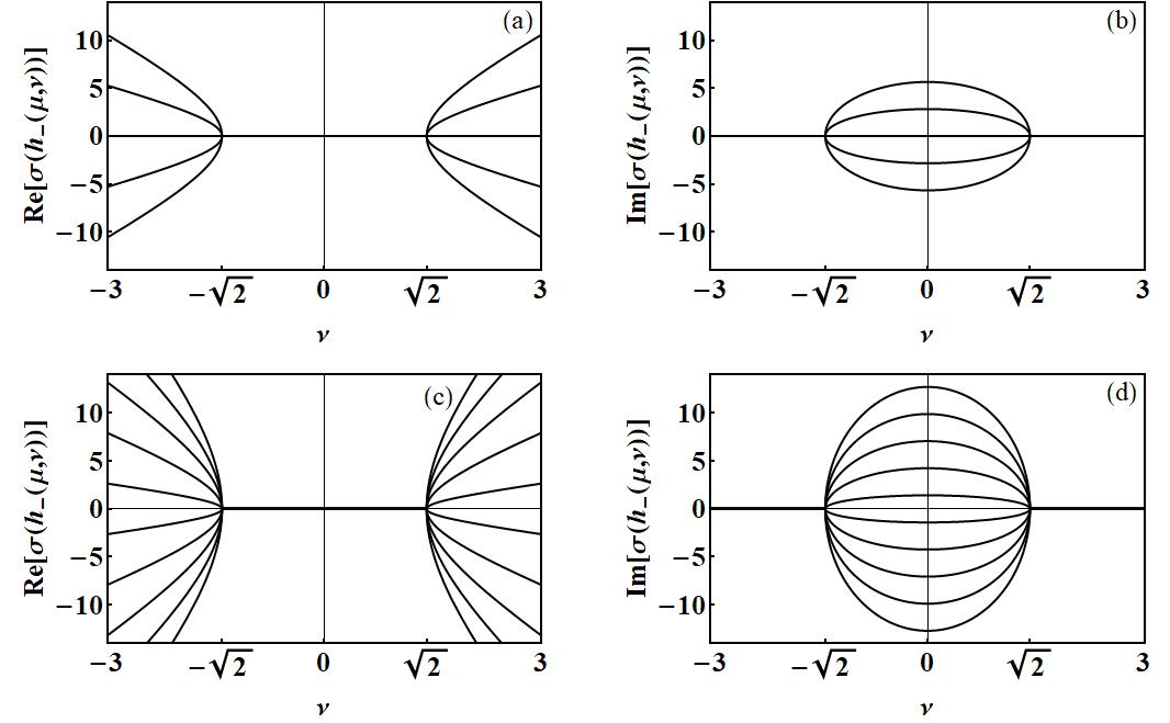
In the following, we analyse the phase structure of the spectrum of the Hamiltonian (39). As a first step, in order to discuss the appearance of EPs in the present model, let us take and . In this manner we get
| (42) |
In Figure 1, we show the behaviour of its spectrum as a function of , for the undeformed Hamiltonian with . Panels (a) and (b) correspond to values of (dimension ), and Panels (c) and (d) correspond to values of (dimension ). In Panels (a) and (c) we display the behaviour of the real part of the eigenvalues. In Panels (b) and (d), the imaginary part of the eigenvalues is depicted. It can be seen the presence of EPs of order 2 and 5 at , for the and cases, respectively.
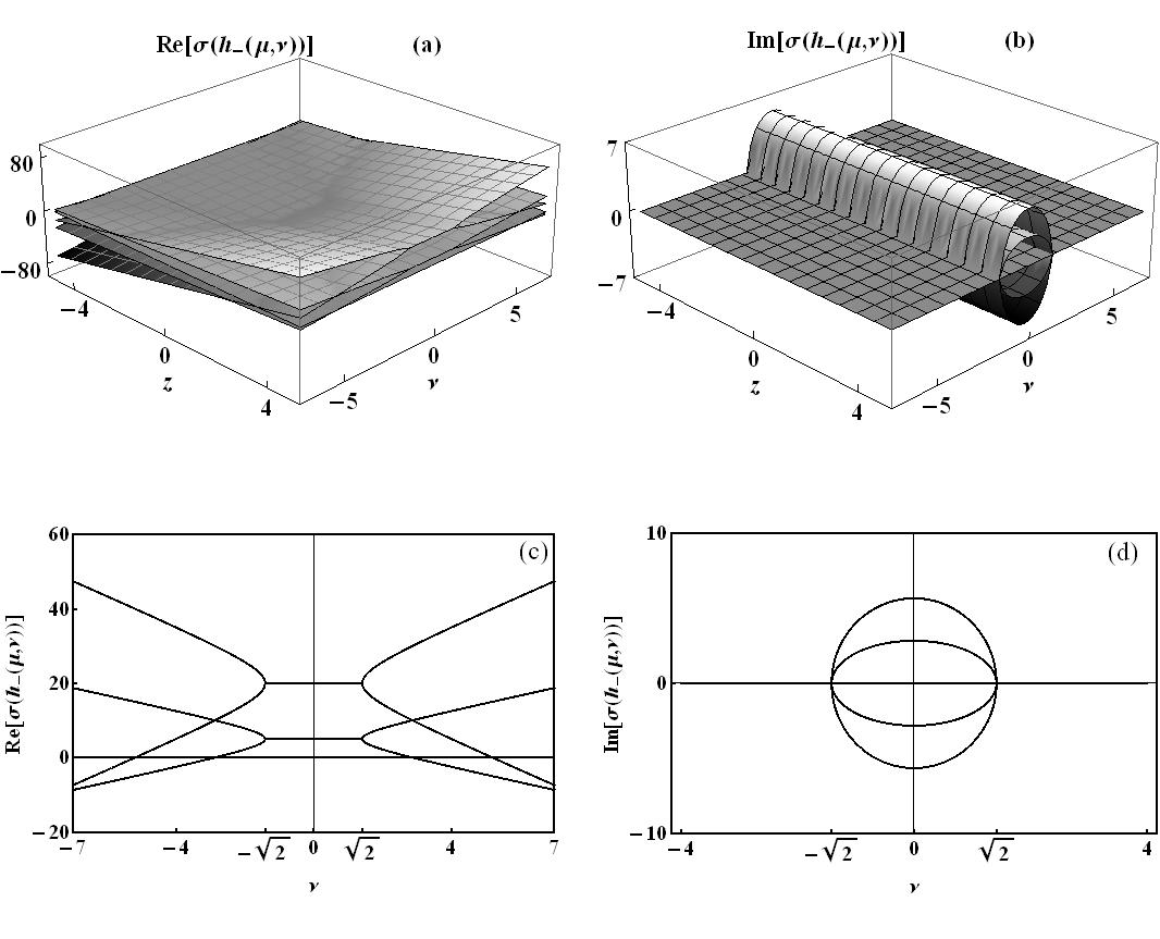
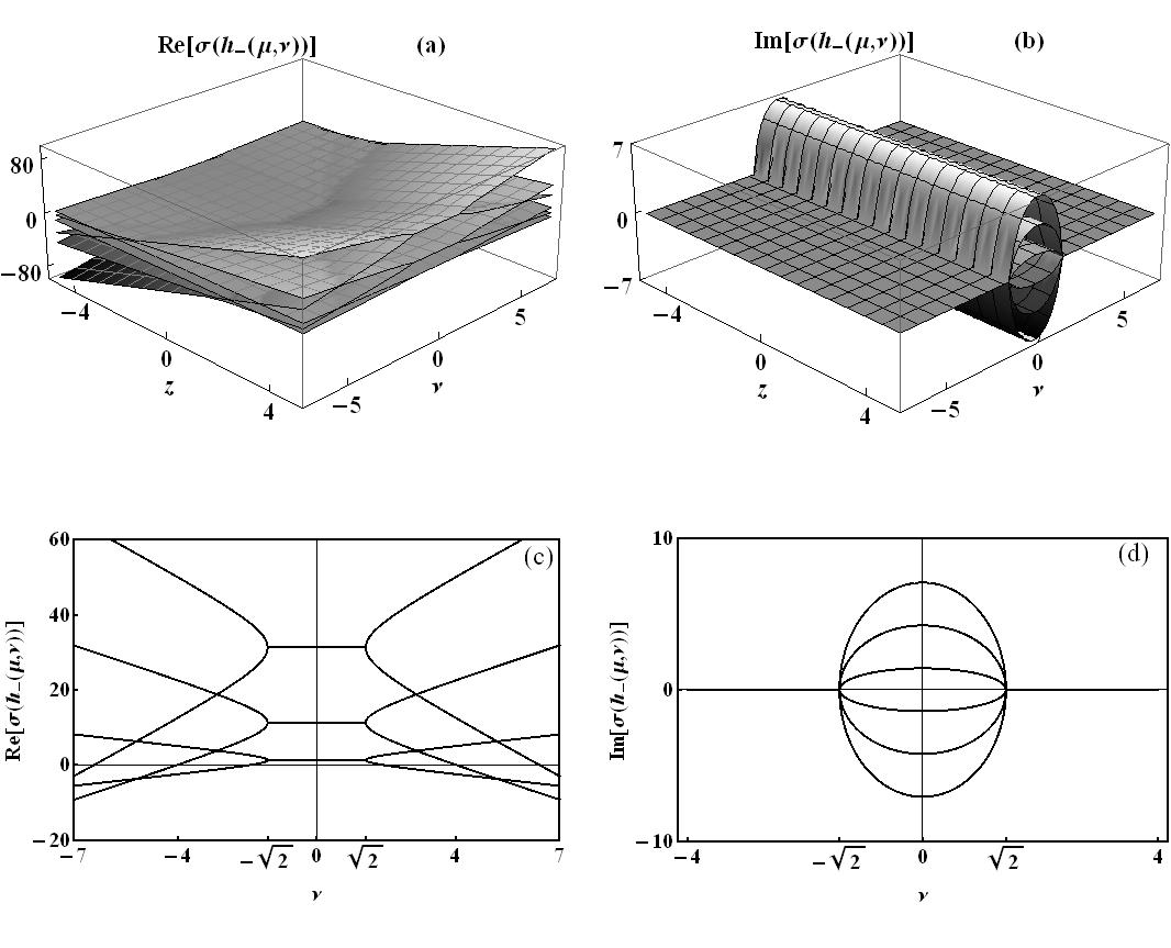
In Figures 2 and 3, we display the spectrum of the deformed Hamiltonian in units of , as a function of both and the deformation parameter
, for dimensions and . In Panels (a) and (b) we plot the real and the imaginary part of the eigenvalues, respectively.
In Panels (c) and (d), we present the projection for the case . The real and imaginary parts of the eigenvalues are presented in (c) and (d), respectively. The EPs occur at values of .
For the Hamiltonian of (42), , the EPs lie between the region with exact symmetry (real spectrum) and the
region of broken -symmetry, with pairs of complex conjugate energies.
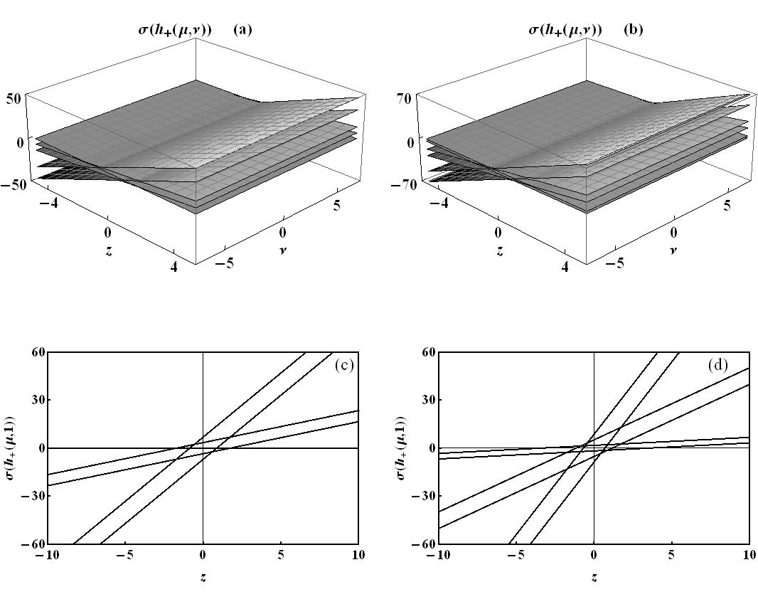
As a second example, let us consider and :
| (43) |
In this case, the spectrum of , , takes real values.
In Figure 4, we plot the spectrum of in units of , as a function of and . Panels (a) and (c) correspond to the results obtained for dimension , while Panels (b) and (d) correspond to the results for dimension . In Panels (c) and (d) we present the projections of the graphs at , as a function of z.
It is important to emphasise that, as a function of , eigenvalues form ‘bands’ composed of two energies. The distance between consecutive bands is governed by the second term of (40). This will be of the outmost relevance when dealing with the applications presented in the next Section.
Finally, we shall consider another family of exactly solvable Hamiltonians written in terms of the generators of , namely
| (44) |
where .
As in the previous cases, by using the similarity transformation given now by the operator (see A for computations) and afterwards by taking the limit , we can map into a Hamiltonian , such that its matrix representation is given in terms of triangular matrices:
| (45) |
As a consequence, we can state the following
Proposition 4. The spectrum of is given by
| (46) |
where
Clearly, for the eigenvalues of of (44) belong to . It can be observed from (46) that for , the characteristic degeneracy of the spectrum of the operator is broken, giving rise again to bands of pairs of parallel lines separated by a controlled gap. Note that the gap is symmetric when resp. , i.e when , for even (odd) dimension. When odd coefficients are zero, i.e. all , we have (resp. ) for even (odd) dimension, thus resulting in a Hamiltonian with degenerate spectrum.
As an specific example, we can consider the Hamiltonians
| (47) |
| (48) |
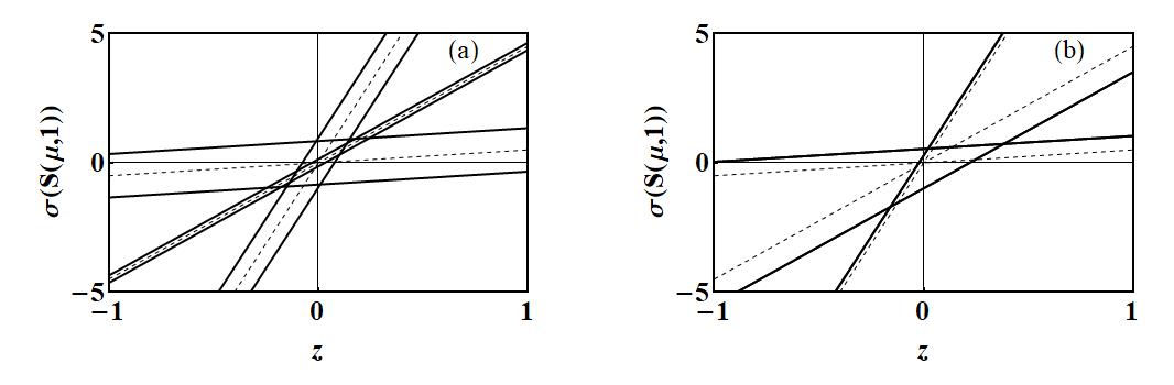
The operators and aare defined by power series with particular values of , with even and odd null coefficients, respectively. In Figure 5 we represent, with solid lines, the spectrum of Hamiltonians of (47) and (48). We have plotted the case for dimension . As a guide, with dashed lines, we plot the spectrum of the Hamiltonian of (44) when . It can be seen from Panel (a) that, the spectrum of has pairs of parallel lines symmetrically separated with respect to the spectrum of by a controlled gap given by , respectively. For we can see in Panel (b) that the degeneracy of is preserved, albeit displaced into a new double degenerate spectrum given by , due to the parity of the function.
4 Applications
It is worth stressing that, recently, the separation in bands of parallel lines has been observed in the spectra of three electrons confined in an asymmetric two-dimensional double well, implemented by a two-centre-oscillator potential. This system turns out to be the cornerstone of two-dimensional (2D) semiconductor-based three-electron hybrid- double-quantum-dot (HDQD) qubits (see [34, 19] and references therein). In the literature, theoretical model Hamiltonians have been developed to reproduce these experimental results [35, 36].
The results presented in the previous Section strongly suggest the possibility of making use of specific -symmetric Hamiltonians defined on the non-standard quantum algebra in order to model these relevant systems. We show in the following that this will be indeed the case.
Let us consider the effective Hamiltonian of [34] given by the equivalent form
| (53) |
where the parameter models the detuning of three-electron hybrid qubits based on GaAs asymmetric double quantum dots, and with coupling constants (in units of [GHz]) [19]. The eigenvalues of the Hamiltonian of (53) can be obtained analytically as the roots of a fourth-degree polynomial:
| (54) |
The explicit form of the coefficients is given in C. For sufficiently large the eigenvalues of the Hamiltonian (53) can be approximated by two sets of eigenvalues:
| (55) |
An effective non-standard quantum algebra Hamiltonian reproducing the behaviour of the spectrum of (53) an be obtained through
| (60) |
with
| (61) |
by identifying the deformation parameter with the detuning, therefore , and by making use of the two-dimensional irreducible representation of the quantum algebra (23) obtained from (9) with .
To obtain an isospectral Hamiltonian to , we construct the symmetry operator of (34), and from it the similarity transformation given by its square root :
| (64) | |||||
being
| (67) |
with
| (70) | |||||
| (73) |
In this way we obtain that
| (76) | |||||
| (79) |
It is straightforward to prove that the eigenvalues of and are just and , respectively.
Moreover, by making use of a second similarity transformation , the Hamiltonian can be arranged as
| (84) | |||||
where
| (87) |
is given by
| (90) | |||||
| (93) |
Figure 6 depicts the spectrum of and as a function of . In Panel (a), the exact eigenvalues of and their approximate values computed from (55) are displayed as a function of with solid and dashed lines, respectively. Panel (b) is devoted to analyse the differences between the energies deduced from the two models, which turn out to be very small under the identification between and the deformation parameter .
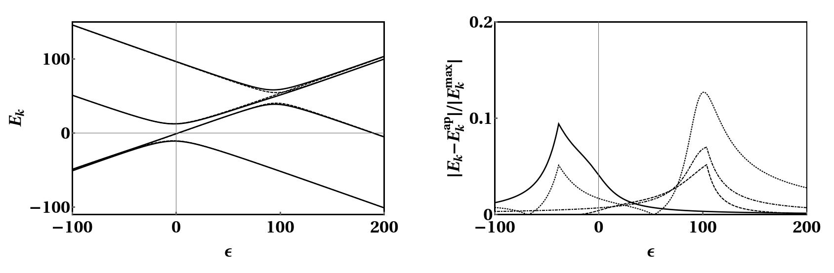
Therefore the previous example shows that realistic physical systems can be modeled by effective -symmetry Hamiltonians constructed from the non-standard algebra, and provided that the model parameters are chosen appropriately.
5 Conclusions and outlook
In this work, we have obtained the analytical expression for the spectrum of a family of -symmetric Hamiltonians defined in terms of the generators of the non-standard quantum algebra under a generic finite-dimensional irreducible representation of the latter [14, 37, 15, 16]. By generalising [16], we have presented a boson realisation of the generators of the algebra such that the co-product map and the commutation relations become invariant under the -transformation. In terms of these operators, we have introduced two families of -symmetry Hamiltonians, given by (36) and (44).
We have shown that the spectrum of the Hamiltonian in (36) exhibits different properties depending on the relative signs of the parameters . When the spectrum of of (36) is real. Nevertheless, when , the spectrum of can include complex conjugate pairs of eigenvalues. Thus, we have two different dynamical phases, the exact -symmetry phase for with real energies, and the one for the broken -symmetry phase for consisting in pairs of complex conjugate eigenvalues. The boundary between these phases, given by , is formed by EPs. At these points, two or more eigenvalues are degenerated and their eigenvectors are coalescent.
On the other hand, the spectrum of the Hamiltonian defined in (44) has been shown to consist, for real parameters, of real eigenvalues. As a characteristic feature of this spectrum, we have illustrated the appearance of bands consisting of pairs of eigenvalues, and we have studied the relation of the parameters of the model with the gap between such bands.
Remarkably enough, this particular band structure has suggested the definition of a non-standard quantum algebra effective model for the spectrum of a realistic system of three-electron hybrid qubits based on GaAs asymmetric double quantum dots [19]. In fact, by identifying the deformation parameter with the detuning of the system, the spectrum of the effective Hamiltonian (61) provides an excellent approximation to the energies of the actual physical system.
Work is in progress concerning the analytical spectra for more general -symmetric Hamiltonians written in terms of the generators of the algebra. Also, their possible role as effective models for other quantum systems beyond the one here presented where the Hopf algebra deformation parameter had a neat physical interpretation.
Appendix A
Appendix B
We shall prove that the coproduct (), the counit (), antipode ( ) maps and the commutation rules amongst the operators have the same structure as those of .
Let us start with the Hopf structure of the operators :
| (97) |
we shall write the maps for in terms of :
| (98) | |||||
For the commutation relations, we have:
| (99) | |||||
Next, we shall prove the invariance of the coproduct and the commutation relations under a symmetry transformation. Let us summarise the transformation properties of the different operators and scalars under -symmetry:
| (100) |
Therefore we have:
In a similar way, we can show that the commutation relations are also invariant under -symmetry transformations:
| (102) | |||||
Appendix C
Acknowledgements
A.B. has been partially supported by Agencia Estatal de Investigación (Spain) under grant PID2019-106802GB-I00/AEI/10.13039/501100011033, and by the Q-CAYLE Project funded by the Regional Government of Castilla y León (Junta de Castilla y León) and by the Ministry of Science and Innovation MICIN through the European Union funds NextGenerationEU (PRTR C17.I1). M.R. is grateful to the Universidad de Burgos for its hospitality. M.R. and R.R. have been partially supported by the grant 11/X982 of the University of La Plata (Argentine).
References
References
- [1] Bender, C. & Boettcher, S. Real Spectra in Non-Hermitian Hamiltonians Having PT Symmetry. Phys. Rev. Lett.. 80, 5243-5246 (1998,6), https://link.aps.org/doi/10.1103/PhysRevLett.80.5243
- [2] Bender, C., Berry, M. & Mandilara, A. Generalized PT symmetry and real spectra. Journal Of Physics A: Mathematical And General.. 35, L467 (2002,7), https://dx.doi.org/10.1088/0305-4470/35/31/101
- [3] Brody, D. Biorthogonal quantum mechanics. Journal Of Physics A: Mathematical And Theoretical.. 47, 035305 (2013,12), https://dx.doi.org/10.1088/1751-8113/47/3/035305
- [4] Bender, C., Gianfreda, M., Özdemir, ,̇ Peng, B. & Yang, L. Twofold transition in PT-symmetric coupled oscillators. Phys. Rev. A. 88, 062111 (2013,12), https://link.aps.org/doi/10.1103/PhysRevA.88.062111
- [5] Beygi, A., Klevansky, S. & Bender, C. Coupled oscillator systems having partial PT symmetry. Phys. Rev. A. 91, 062101 (2015,6), https://link.aps.org/doi/10.1103/PhysRevA.91.062101
- [6] Wen, Z. & Bender, C. -symmetric potentials having continuous spectra. Journal Of Physics A: Mathematical And Theoretical.. 53, 375302 (2020,8), https://dx.doi.org/10.1088/1751-8121/aba468
- [7] Bender, C. & Jones, H. Interactions of Hermitian and non-Hermitian Hamiltonians. Journal Of Physics A: Mathematical And Theoretical.. 41, 244006 (2008,6), https://dx.doi.org/10.1088/1751-8113/41/24/244006
- [8] Mostafazadeh, A. Pseudo Hermitian Representation of Quantum Mechanics. International Journal Of Geometric Methods In Modern Physics. 7, 1191-1306 (2010), https://doi.org/10.1142/S0219887810004816
- [9] Soley, M., Bender, C. & Stone, A. Experimentally Realizable PT Phase Transitions in Reflectionless Quantum Scattering. Phys. Rev. Lett.. 130, 250404 (2023,6), https://link.aps.org/doi/10.1103/PhysRevLett.130.250404
- [10] Ramy, E., Makris, K., Khajavikhan, M., Musslimani, Z., Rotter, S. & Demetrios N. Christodoulides Non-Hermitian physics and PT symmetry. Nature Physics. 14, 11-19 (2018), https://doi.org/10.1038/nphys4323
- [11] Berry, M. Physics of Nonhermitian Degeneracies. Czechoslovak Journal Of Physics. 54, 1039-1047 (2004), https://doi.org/10.1023/B:CJOP.0000044002.05657.04
- [12] Miri, M. & Andrea Alù Exceptional points in optics and photonics. Science. 363, 7709 (2019), https://www.science.org/doi/abs/10.1126/science.aar7709
- [13] Znojil, M. Exceptional points and domains of unitarity for a class of strongly non-Hermitian real-matrix Hamiltonians. Journal Of Mathematical Physics. 62, 052103 (2021,5), https://doi.org/10.1063/5.0041185
- [14] Demidov, E., Manin, Y., Mukhin, E. & Zhdanovich, D. Non-Standard Quantum Deformations of GL(n) and Constant Solutions of the Yang-Baxter Equation. Progress Of Theoretical Physics Supplement. 102 pp. 203-218 (1990,3), https://doi.org/10.1143/PTPS.102.203
- [15] Ballesteros, A. & Herranz, F. Universal R-matrix for non-standard quantum. Journal Of Physics A: Mathematical And General. 29, L311 (1996,7), https://dx.doi.org/10.1088/0305-4470/29/13/001
- [16] Ballesteros, A., Herranz, F. & Negro, J. Boson representations, non-standard quantum algebras and contractions. Journal Of Physics A: Mathematical And General. 30, 6797 (1997)
- [17] Ballesteros, A., Herranz, F., Negro, J. & Nieto, L. Twist maps for non-standard quantum algebras and discrete Schrödinger symmetries. Journal Of Physics A: Mathematical And General. 33, 4859 (2000,7), https://dx.doi.org/10.1088/0305-4470/33/27/303
- [18] Ballesteros, A. & Herranz, F. Lie bialgebra quantizations of the oscillator algebra and their universal R-matrices. Journal Of Physics A: Mathematical And General. 29, 4307 (1996)
- [19] Jang, W., Cho, M., Jang, H., Kim, J., Park, J., Kim, G., Kang, B., Jung, H., Umansky, V. & Kim, D. Single-Shot Readout of a Driven Hybrid Qubit in a GaAs Double Quantum Dot. Nano Letters. 21, 4999-5005 (2021),
- [20] Gilmore, R. Lie Groups, Lie Algebras, and Some of Their Applications. (Dover Publications, Inc. New York,2005)
- [21] Dyson, F. General Theory of Spin-Wave Interactions. Phys. Rev.. 102, 1217-1230 (1956,6), https://link.aps.org/doi/10.1103/PhysRev.102.1217
- [22] Klein, A. & Marshalek, E. Boson realizations of Lie algebras with applications to nuclear physics. Rev. Mod. Phys.. 63, 375-558 (1991,4), https://link.aps.org/doi/10.1103/RevModPhys.63.375
- [23] Assis, P. & Fring, A. Non-Hermitian Hamiltonians of Lie algebraic type. Journal Of Physics A: Mathematical And Theoretical.. 42, 015203 (2008,11), https://dx.doi.org/10.1088/1751-8113/42/1/015203
- [24] Assis, P. & Fring, A. Metrics and isospectral partners for the most generic cubic -symmetric non-Hermitian Hamiltonian. Journal Of Physics A: Mathematical And Theoretical. 41 pp. 244001 (2007), https://api.semanticscholar.org/CorpusID:17965936.
- [25] Higgs, P. Dynamical symmetries in a spherical geometry. I. Journal Of Physics A: Mathematical And General.. 12, 309 (1979,3), https://dx.doi.org/10.1088/0305-4470/12/3/006
- [26] Debergh, N. The relation between polynomial deformations of sl(2,R) and quasi-exact solvability. Journal Of Physics A: Mathematical And General.. 33, 7109 (2000,10), https://dx.doi.org/10.1088/0305-4470/33/40/308
- [27] Debergh, J. & Bossche, B. Polynomial Deformations of sl(2, ) in a three-dimensional invariant subspace of monomials. Modern Physics Letters A.. 18, 1013-1022 (2003)
- [28] Ballesteros, A., Civitarese, O., Herranz, F. & Reboiro, M. Generalized rotational Hamiltonians from nonlinear angular momentum algebras. Phys. Rev. C. 75, 044316 (2007,4), https://link.aps.org/doi/10.1103/PhysRevC.75.044316
- [29] Chari, V. & Pressley, A. A guide to quantum groups. (Cambridge University Press, Cambridge,1994)
- [30] Majid, S. Foundations of quantum group theory. (Cambridge University Press, Cambridge,1995)
- [31] Drinfel’d, V. Quantum Groups. (American Mathematical Society,1987)
- [32] Jimbo, M. A q-difference analogue of U(g) and the Yang-Baxter equation. Letters In Mathematical Physics. 10, 63-69 (1985), http://dx.doi.org/10.1007/BF00704588
- [33] Ramirez, R. & Reboiro, M. Dynamics of finite dimensional non-hermitian systems with indefinite metric. Journal Of Mathematical Physics. 60, 012106 (2019)
- [34] Shi, Z., Simmons, C., Ward, D., Prance, J., Wu, X., Koh, T., Gamble, J., Savage, D., Lagally, M., Friesen, M., Coppersmith, S. & Eriksson, M. Fast coherent manipulation of three-electron states in a double quantum dot. Nature Communications., 3020 (2014)
- [35] Yannouleas, C. & Landman, U. Wigner molecules and hybrid qubits. Journal Of Physics: Condensed Matter.. 34, 21LT01 (2022,3), https://dx.doi.org/10.1088/1361-648X/ac5c28
- [36] Lemaalem, B., Zahidi, Y. & Jellal, A. Band structures of hybrid graphene quantum dots with magnetic flux. Physics Letters A. 426 pp. 127898 (2022), https://www.sciencedirect.com/science/article/pii/S0375960121007635
- [37] Abdesselam, B., Chakrabarty, A. & Chakrabarty, R. Irreducible representations of the Jordian Quantum Algebra Uh(sl(2)) via a nonlinear map VIA A. Modern Physics Letters A. 11, 2883-2891 (1996), https://doi.org/10.1142/S0217732396002861
- [38] Abramowitz, M. & Stegun Handbook of Mathematical Functions with Formulas, Graphs, and Mathematical Tables. (I. A. (Eds.). new York,1972)