ParamANN: A Neural Network to Estimate Cosmological Parameters for $\Lambda$CDM Universe using Hubble Measurements

Abstract

In this article, we employ a machine learning (ML) approach for the estimations of four fundamental parameters, namely, the Hubble constant ($H_{0}$), matter ($\Omega_{0m}$), curvature ($\Omega_{0k}$) and vacuum ($\Omega_{0\Lambda}$) densities of non-flat $\Lambda$CDM model. We use $53$ Hubble parameter values measured by differential ages (DA) and baryon acoustic oscillations (BAO) techniques in the redshift interval $0.07\leq z\leq 2.36$. We create an artificial neural network (called ParamANN) and train it with simulated values of $H(z)$ using various sets of $H_{0}$, $\Omega_{0m}$, $\Omega_{0k}$, $\Omega_{0\Lambda}$ parameters chosen from different and sufficiently wide prior intervals. We use a correlated noise model in the analysis. We demonstrate accurate validation and prediction by ParamANN. ParamANN provides an excellent cross-check for the validity of the $\Lambda$CDM model and alleviates the Hubble tension problem which has been reported earlier in the literature. We obtain $H_{0}=66.11\pm 2.59$ $\rm{kmMpc^{-1}sec^{-1}}$, $\Omega_{0m}=0.3359\pm 0.0814$, $\Omega_{0k}=0.0237\pm 0.1248$ and $\Omega_{0\Lambda}=0.6405\pm 0.0861$ by using the trained network. These parameter values agree very well with the results of global CMB observations of Planck collaboration.

Keywords: Hubble parameter - Cosmological density parameters - Machine learning

1 Introduction

Our universe consists of visible matter, radiation as well as two mysterious components, i.e., dark matter (Zwicky, 2017; Freeman, 1970; Lacki & Beacom, 2010) and dark energy (Riess et al., 1998; Perlmutter et al., 1999). Although, the properties of both visible and dark matters are similar to each other, the latter does not interact with anything except gravitation. Moreover, dark energy, which explains the accelerated expansion of the universe, follows the property of negative pressure. The simplest cosmological model to express our universe is $\Lambda$ cold dark matter ($\Lambda$CDM) model, where $\Lambda$ defines the cosmological constant which was first envisioned by Albert Einstein (1917). This cosmological constant or vacuum is the simplest form of dark energy. Following this $\Lambda$CDM model, recent observations (Planck collaboration VI, 2020) of cosmic microwave background (CMB) radiation reveal spatially flatness of our present universe and measure the rediation density of the present universe which is of the order of $10^{-4}$. Therefore, our present universe shows that the matter (specifically dark matter) and vacuum densities are the major components of the universe (Planck collaboration VI, 2020).

Recent observations of CMB data agree well with the flat $\Lambda$CDM universe. According to CMB observations, our present universe comprises $4.6\%$ visible matter, $24\%$ dark matter, and $71.4\%$ vacuum energy approximately. However, researchers raise their concerns with $\Lambda$CDM model for the final interpretation of the universe. Zunckel & Clarkson (2008) verify the acceptance of $\Lambda$CDM model using ‘litmus test’. Their results show the disagreement with $\Lambda$ as the dark energy component of the universe as well as prevent other dark energy models used in their analysis. Measurements of Canada-France-Hawaii-Telescope Lensing Survey (Macaulay et al., 2013; Raveri, 2016) raise a tension with the estimations of Planck collaboration VI (2020). Testing of Copernican principle (Uzan et al., 2008; Valkenburg et al., 2014) is also a well-known procedure to examine the existence and evolution of dark energy. For the null test of flat $\Lambda$CDM universe, $Om(z_{i},z_{j})$ and $Omh^{2}(z_{i},z_{j})$ diagnostics (Sahni et al., 2008; Shafieloo et al., 2012; Sahni et al., 2014) can be probed by using Hubble measurements directly. Zheng et al. (2016) use $Om(z_{i},z_{j})$ and $Omh^{2}(z_{i},z_{j})$ to estimate the matter density by using observed $H(z)$ values as well as assuming the prior value of Hubble constant for three cosmological models (i.e., $\Lambda$CDM, wCDM, CPL (Chevalier & Polarski, 2001; Linder, 2003)) of flat universe. Shahalam et al. (2015) apply the $Om$ diagnostic in scalar field models as well as distinguish the $\Lambda$CDM model from non-minimally coupled scalar field, phantom field, and quintessence models. Leaf & Melia (2017) analyze only differential ages (DA) Hubble measurements using a two-point diagnostic for model comparison since the measurements of $H(z)$ from cosmic chronometers are model independent. Geng et al. (2018) use $H(z)$ data measured by DA and baryon acoustic oscillation (BAO) techniques to constrain the cosmological parameters as well as quantify the impact of future $H(z)$ measurements in the estimation of these parameters. The recent literatures, e.g., (Gómez-Valent & Amendola, 2018; Ryan et al., 2018, 2019; Cao et al., 2021; Cao & Ratra, 2022), effectively use the low redshift data (i.e., DA+BAO Hubble data, QSO angular size, Pantheon, DES supernova etc.) to analyse the various cosmological models.

In spite of excellent agreement of the $\Lambda$CDM model with the observations as discussed above, there are still some indications that the $\Lambda$CDM model may not be entirely consistent with the observations. One such area of incompatibility is known as the so-called problem of ‘Hubble tension’. The tension was reported since $H_{0}$ values estimated by local and global observations do not agree with each other. The value of $H_{0}$ constrained by Planck collaboration VI (2020) shows $\sim 3.6\sigma$ tension with the same measured by local observational data, in which local measurements of $H_{0}$ demand the higher value of this parameter. Recent local observations of Hubble Space Telescope (HST) (Riess et al., 2018, 2019; Riess, 2020; Riess et al., 2021, 2022) estimate the value of Hubble constant which shows approximately $4$-$5\sigma$ tension with Planck’s estimation of $H_{0}$. Local measurement of $H_{0}$ by using gravitationally lensed quasars (i.e., H0LiCOW (Wong et al., 2019)) shows $\sim 5.3\sigma$ tension with Planck’s $H_{0}$ value. Di Valentino (2021) estimated the value of $H_{0}$ by combining 23 local measurements of this parameter and this estimation shows $5.9\sigma$ tension with $H_{0}$ constrained by CMB observations (Planck collaboration VI, 2020). An alternative method to estimate of $H_{0}$ value (along with other cosmological parameters) as is done in this work is of utmost importance in the contemporary cosmological analysis.

It is worth mentioning that the problem of Hubble tension seems to be somewhat perplexing in nature. On one hand, some observations (de Jaeger et al., 2022) indicate a high value of $H_{0}$. Riess et al. (2022) constrain $H_{0}=73.04$ $\rm{kmMpc^{-1}sec^{-1}}$ with a uncertainty of 1.04 $\rm{kmMpc^{-1}sec^{-1}}$ using Cepheid-SNe samples for their baseline redshift range $0.0233<z<0.15$. The Pantheon+ analysis (Brout et al., 2022) use 1550 distinct type Ia Supernovae in the redshift interval 0.001 to 2.26 and report the $H_{0}=73.5\pm 1.1$ $\rm{kmMpc^{-1}sec^{-1}}$. Thus it appears that the Hubble tension extends up to a redshift of 2.26 if Supernovae data is used. Interestingly, using the red giant branch (TRGB) calibration to a sample of Type Ia Supernovae, Freedman (2021) reports $H_{0}=69.8\pm 0.6$ (stat) $\pm 1.6$ (sys) $\rm{kmMpc^{-1}sec^{-1}}$ which is consistent with the $H_{0}$ value estimated by Planck collaboration VI (2020). Kelly et al. (2023) obtain $H_{0}=64.8^{+4.4}_{-4.3}$ $\rm{kmMpc^{-1}sec^{-1}}$ by using eight lens models and $66.6^{+4.1}_{-3.3}$ $\rm{kmMpc^{-1}sec^{-1}}$ from two preferred models. A recent article (Mukherjee et al., 2020) report $H_{0}=67.6^{+4.3}_{-4.2}$ $\rm{kmMpc^{-1}sec^{-1}}$ using VLBI and gravitational wave observations from bright binary black hole GW190521 and conclude that the value is consistent with the Planck observations. These relax the tension. At the backdrop of such diverse indications from the observations it is a very important task to measure the cosmological parameters in an as much general framework (i.e., measuring all the independent cosmological parameters) as possible using the favoured $\Lambda$CDM model and new observational data. In this article, we use $H(z)$ observations alone to constrain the parameters using the artificial intelligence (AI) as the driving engine.

We use AI to estimate the Hubble constant ($H_{0}$) and today’s density parameters (i.e., matter ($\Omega_{0m}$), curvature ($\Omega_{0k}$), vacuum ($\Omega_{0\Lambda}$)) for $\Lambda$CDM universe from the $H(z)$ values measured by DA and BAO techniques. We create an ANN (hereafter ParamANN) for modelling a direct mapping function between the observed $H(z)$ and corresponding four parameters of the $\Lambda$CDM universe. The density parameters estimated by ParamANN indicate the spatially flat $\Lambda$CDM universe which is consistent with the results of Planck collaboration VI (2020). Moreover, Hubble constant predicted by ParamANN agrees excellently with the Planck’s estimation of the same. Therefore, we do not see the problem of Hubble tension in the Hubble data.

Primary motivations of our current article stem from the perspective of both theoretical and observational fronts. From the observational side, the problem like Hubble tension (Planck collaboration VI, 2020; Riess et al., 2018, 2019; Riess, 2020; Riess et al., 2021, 2022; Wong et al., 2019; Di Valentino, 2021; de Jaeger et al., 2022; Brout et al., 2022) exists and needs further understanding using various types of available data. AI has become one of the promising tool to investigate the observed data since an ML model can predict (in principle) a complicated function once it has been trained successfully. Moreover, there are several articles in the literature, e.g. (Macaulay et al., 2013; Raveri, 2016; Shafieloo et al., 2012; Sahni et al., 2014; Zheng et al., 2016; Linder, 2003; Shahalam et al., 2015; Leaf & Melia, 2017; Geng et al., 2018; Gómez-Valent & Amendola, 2018; Bengaly et al., 2023; Liu et al., 2019; Arjona & Nesseris, 2020; Mukherjee et al., 2022; Garcia et al., 2023), which try to measure the cosmological parameters assuming flat spatial curvature of our universe. However, it is also important to ask whether we can estimate these cosmological parameters by relaxing the assumption of the flatness of the universe. In this article, we motivate ourselves to estimate cosmological density parameters along with today’s Hubble parameter value for a general non-flat $\Lambda$CDM universe. From the observational perspective, many new experiments are being proposed (e.g., Echo (aka CMB-Bharat), CCAT-prime (Stacey et al., 2018), PICO (Hanany et al., 2019), Lite-Bird (Hazumi et al., 2020), SKA (Dewdney et al., 2009)) which has lower noise level implying the model parameters of a theory can be measured with higher accuracy. The higher accuracy of the future generation observations demand accurate constraining of cosmological parameters to distinguish between different models of the universe which is a major step to find a better and more accurate theoretical understanding of the physics of the universe.

In the modern era, ML techniques are utilized as the powerful tools to analyze the observational data of the several fields in cosmology (Olvera et al., 2022). Instead of Metropolis-Hastings algorithm, artificial neural network (ANN) can be used as an alternative approach for the Bayesian inference in cosmology effectively reducing the computational time (Graff et al., 2012; Moss, 2020; Hortua et al., 2020; Gómez-Vargas et al., 2021). Moreover, ANNs can be performed for the non-parametric reconstructions of cosmological functions (Escamilla-Rivera et al., 2020; Wang et al., 2020a; Dialektopoulos et al., 2022; Gómez-Vargas et al., 2023). For the estimations of cosmological parameters by using CMB data, Mancini et al. (2022) implement several types of ANN and show the less computational time in the Bayesian process by using these ANNs. Baccigalupi et al. (2000) utilize ANN to separate different types of foregrounds (e.g., thermal dust emissions, galactic synchrotron, and radiation emitted by galaxy clusters) from CMB signal. Petroff et al. (2020) develop a Bayesian spherical convolutional neural network (CNN) to recover the CMB anisotropies from the foreground contaminations. Using a CNN, Shallue & Eisenstein (2023) reconstruct the cosmological initial conditions from the late-time and non-linearly evolved density fields. ML can be used to reconstruct full sky CMB temperature anisotropies from the partial sky maps (Chanda & Saha, 2021; Pal et al., 2023). Khan & Saha (2023) develop an ANN to estimate the dipole modulation from the foreground cleaned CMB temperature anisotropies. In our previous article (Pal & Saha, 2023), we use a CNN to recover full sky $E$- and $B$-modes polarizations from the partial sky maps avoiding the so-called $E$-to-$B$ leakage. Wang et al. (2020b) use ANN to estimate cosmological parameters from the temperature power spectrum of CMB. Bengaly et al. (2023) employ ML algorithm to constrain the Hubble constant ($H_{0}$) by using DA Hubble measurements. Moreover, the recent literature, e.g. (Liu et al., 2019; Arjona & Nesseris, 2020; Mukherjee et al., 2022; Garcia et al., 2023; Wang et al., 2021; Liu et al., 2021), also perform the ML techniques to analyze the low redshift data (i.e., Hubble measurements (DA+BAO), Type Ia Supernovae etc.) for constraining the cosmological parameters of present universe.

We organize our article as the following. In section 2, we describe the fundamental relation between Hubble parameter and redshift for $\Lambda$CDM universe. We discuss the methodology of our analysis in section 3. In section 3.1, we present the Hubble parameters measured by DA and BAO techniques. In section 3.2, we discuss the procedure to generate the samples of four fundamental parameters (i.e., $H_{0}$ ,$\Omega_{0m}$ ,$\Omega_{0k}$, $\Omega_{0\Lambda}$) and the corresponding mock values of $H(z)$. In section 3.3, we describe the addition of noises to these mock $H(z)$ values. We express the deep learning procedure of ParamANN in section 3.4. In section 3.4.1, we discuss about the architecture of ParamANN. In section 3.4.2, we describe the preprocessing of input data for ParamANN. In section 3.4.3, we present the loss function employed in the ParamANN. After that, in section 3.4.4, we provide the detailed descriptions about the training and prediction processes of ParamANN. We show the results, predicted by ParamANN, with detailed analysis in section 4. We present the predictions of ParamANN for the test set in section 4.1. We show the results predicted by ParamANN for observed Hubble data in section 4.2. In section 4.2.1, we present the values of Hubble constant and the density parameters with their corresponding uncertainties which are obtained by trained ParamANN for observed $H(z)$ data as well as in section 4.2.2 we present the Hubble parameter curve using these estimated parameter values comparing with the same obtained by using the results of Planck collaboration VI (2020). Finally, in section 5, we conclude our current analysis with the beneficial discussions of this new work.

2 Formalism

Einstein’s equations which can be encapsulated into a compact form using tensor notations follow

$$G_{\mu\nu} = -\frac{8\pi G}{c^{4}}T_{\mu\nu},$$ (1)

where Einstein’s tensor $G_{\mu\nu}$ is determined by some suitable second order derivative functions of the metric tensor $g_{\mu\nu}$ with respect to the coordinates. In equation 1, $G$ denotes the universal gravitational constant, $c$ is the velocity of light in vacuum, and $T_{\mu\nu}$ defines the energy-momentum tensor.

In spherical coordinates, the Friedmann-Robertson-Walker (FRW) line element can be written as

$$\differential s^{2} = c^{2}\differential t^{2}-a^{2}(t)\left[\frac{\differential r^{2}}{1-kr^{2}}+r^{2}\left(\differential r^{2}+\sin^{2}\theta\differential\phi^{2}\right)\right],$$ (2)

where $r,\theta$, and $\phi$ are the comoving coordinates of the spherical space of the universe. In equation 2, $a(t)$ and $k$ define the cosmological scale factor and the curvature constant of the universe respectively. Moreover, positive, negative, and zero values of $k$ indicate spatially closed, open, and flat universes respectively.

Using equations 1 and 2, we obtain two well-known Friedmann equations which are expressed as

$$\frac{1}{a^{2}(t)}\left[\left(\derivative{a}{t}\right)^{2}+kc^{2}\right] = \frac{8\pi G}{3}\rho(t),$$ (3)

$$\frac{2}{a(t)}\derivative[2]{a}{t}+\frac{1}{a^{2}(t)}\left[\left(\derivative{a}{t}\right)^{2}+kc^{2}\right] = -\frac{8\pi G}{c^{2}}P(t),$$ (4)

where $\rho(t)$ and $P(t)$ denote the density and gravitational pressure of the universe respectively.

Using equations 3 and 4 as well as the equation of state $P(t)=\omega c^{2}\rho(t)$, we obtain the energy-momentum conservation law which is given by

$$\partialderivative{\rho}{t}+3\left(1+\omega\right)H(t)\rho(t) = 0,$$ (5)

where $\omega$ denotes the equation of state parameter and $H(t)$ represents the Hubble parameter which is defined by $\frac{1}{a(t)}\derivative{a}{t}$. We note that $\omega=0,\frac{1}{3}$, and $-1$ represent the equation of state for matter, radiation and vacuum densities of the universe respectively. Using equation 5, the density components of the universe can be expressed as

$$\rho_{m} = \rho_{0m}\left(1+z\right)^{3},$$ (6)

$$\rho_{r} = \rho_{0r}\left(1+z\right)^{4},$$ (7)

$$\rho_{\Lambda} = \rho_{0\Lambda},$$ (8)

where $z$ denotes the redshift and ‘0’ stands for present universe (i.e., $z=0$). In equations 6, 7 and 8, subscript notations $m,r$ and $\Lambda$ define the matter, radiation and vacuum densities. Moreover, redshift is related to scale factor as $(1+z)=a_{0}/a$.

Neglecting the radiation density for late time universe, equation 3 can be written as

$$\Omega_{m}+\Omega_{k}+\Omega_{\Lambda} = 1.$$ (9)

In equation 9, $\Omega$ denotes the density parameter which is defined by $\rho/\rho_{c}$ for matter and vacuum densities, where $\rho_{c}$ is called the critical density which is expressed as $3H^{2}/8\pi G$. However, the curvature density parameter ($\Omega_{k}$) is defined by $-kc^{2}/a^{2}H^{2}$.

Using equations 6 and 7 in equation 9, the Hubble parameter for $\Lambda$CDM universe is expressed by

$$H^{2}(z) = H^{2}_{0}\left[\Omega_{0m}\left(1+z\right)^{3}+\Omega_{0k}\left(1+z\right)^{2}+\Omega_{0\Lambda}\right],$$ (10)

where $\Omega_{0m}$ and $\Omega_{0\Lambda}$ are the matter and vacuum density parameters in the present universe respectively. Moreover, $\Omega_{0k}$ is today’s curvature density parameter which is specified as $-kc^{2}/a^{2}_{0}H_{0}^{2}$. Zero value of $\Omega_{0k}$ specifies a spatially flat universe. Positive and negative values of $\Omega_{0k}$ define the open and closed universes respectively. At present universe, i.e. $z=0$, equation 10 provides

$$\Omega_{0m}+\Omega_{0k}+\Omega_{0\Lambda} = 1.$$ (11)

Using equation 11, to apply the condition of present universe on the curvature density parameter, equation 10 can be written as

$$H^{2}(z) = H^{2}_{0}\left[\Omega_{0m}\left(1+z\right)^{3}+\left(1-\Omega_{0m}-\Omega_{0\Lambda}\right)\left(1+z\right)^{2}+\Omega_{0\Lambda}\right].$$ (12)

Equation 12 contains three independent parameters $H_{0}$, $\Omega_{0m}$, and $\Omega_{0\Lambda}$. However, the curvature density parameter $\Omega_{0k}$ depends on $\Omega_{0m}$ and $\Omega_{0\Lambda}$ by equation 11. This equation 11 represents the theoretical model of Hubble parameters at different redshifts for a given set of values of $H_{0}$, $\Omega_{0m}$, and $\Omega_{0\Lambda}$.

3 Methodology

In this section, firstly we discuss about the observed Hubble data (available in the range $0.07\leq z\leq 2.36$). Then, we describe the procedure to simulate the mock values of H(z) as well as the noise addition to these mock H(z) data. Thereafter, we provide the descriptions about the deep learning of neural network used in our analysis.

Table 1: Table shows the Hubble parameters ($H(z)$) and corresponding uncertainties ($\sigma_{H(z)}$) in $\rm{kmMpc^{-1}sec^{-1}}$ at different redshifts measured by DA and BAO techniques. We consider the covariances for the Hubble data which are shown with bold fonts in this table. We refer the section 3.3 for the detailed discussions regarding covariances between $H(z)$ data.

DA technique BAO technique $z$ $H(z)$ $\sigma_{H(z)}$ Reference $z$ $H(z)$ $\sigma_{H(z)}$ Reference $0.07$ $69$ $19.6$  Zhang et al. (2014) $0.24$ $79.69$ $2.99$  Gaztañaga et al. (2009) $0.09$ $69$ $12$  Jimenez et al. (2003) $0.30$ $81.7$ $6.22$  Oka et al. (2014) $0.12$ $68.6$ $26.2$  Zhang et al. (2014) $0.31$ $78.18$ $4.74$  Wang et al. (2017) $0.17$ $83$ $8$  Simon et al. (2005) $0.34$ $83.8$ $3.66$  Gaztañaga et al. (2009) $\bf{0.1791}$ $\bf{75}$ $\bf{4}$  Moresco et al. (2012) $0.35$ $82.7$ $8.4$  Chuang & Wang (2013) $\bf{0.1993}$ $\bf{75}$ $\bf{5}$  Moresco et al. (2012) $0.36$ $79.94$ $3.38$  Wang et al. (2017) $0.2$ $72.9$ $29.6$  Zhang et al. (2014) $\bf{0.38}$ $\bf{81.5}$ $\bf{1.9}$  Alam et al. (2017) $0.27$ $77$ $14$  Simon et al. (2005) $0.4$ $82.04$ $2.03$  Wang et al. (2017) $0.28$ $88.8$ $36.64$  Zhang et al. (2014) $0.43$ $86.45$ $3.97$  Gaztañaga et al. (2009) $\bf{0.3519}$ $\bf{83}$ $\bf{14}$  Moresco et al. (2012) $0.44$ $84.81$ $1.83$  Wang et al. (2017) $\bf{0.3802}$ $\bf{83}$ $\bf{13.5}$  Moresco et al. (2016) $0.48$ $87.79$ $2.03$  Wang et al. (2017) $\bf{0.4004}$ $\bf{77}$ $\bf{10.2}$  Moresco et al. (2016) $\bf{0.51}$ $\bf{90.4}$ $\bf{1.9}$  Alam et al. (2017) $\bf{0.4247}$ $\bf{87.1}$ $\bf{11.2}$  Moresco et al. (2016) $0.52$ $94.35$ $2.64$  Wang et al. (2017) $\bf{0.4497}$ $\bf{92.8}$ $\bf{12.9}$  Moresco et al. (2016) $0.56$ $93.34$ $2.3$  Wang et al. (2017) $0.47$ $89$ $34$  Ratsimbazafy et al. (2017) $0.57$ $96.8$ $3.4$  Anderson et al. (2014) $\bf{0.4783}$ $\bf{80.9}$ $\bf{9}$  Moresco et al. (2016) $0.59$ $98.48$ $3.18$  Wang et al. (2017) $\bf{0.5929}$ $\bf{104}$ $\bf{13}$  Moresco et al. (2012) $0.6$ $87.9$ $6.1$  Blake et al. (2012) $\bf{0.6797}$ $\bf{92}$ $\bf{8}$  Moresco et al. (2012) $\bf{0.61}$ $\bf{97.3}$ $\bf{2.1}$  Alam et al. (2017) $\bf{0.7812}$ $\bf{105}$ $\bf{12}$  Moresco et al. (2012) $0.64$ $98.82$ $2.98$  Wang et al. (2017) $\bf{0.8754}$ $\bf{125}$ $\bf{17}$  Moresco et al. (2012) $0.73$ $97.3$ $7$  Blake et al. (2012) $0.88$ $90$ $40$  Stern et al. (2010) $2.3$ $224$ $8$  Busca et al. (2013) $0.9$ $117$ $23$  Simon et al. (2005) $2.33$ $224$ $8$  Bautista et al. (2017) $\bf{1.037}$ $\bf{154}$ $\bf{20}$  Moresco et al. (2012) $2.34$ $222$ $7$  Delubac et al. (2015) $1.3$ $168$ $17$  Simon et al. (2005) $2.36$ $226$ $8$  Font-Ribera et al. (2014) $\bf{1.363}$ $\bf{160}$ $\bf{33.6}$  Moresco (2015) $1.43$ $177$ $18$  Simon et al. (2005) $1.53$ $140$ $14$  Simon et al. (2005) $1.75$ $202$ $40$  Simon et al. (2005) $\bf{1.965}$ $\bf{186.5}$ $\bf{50.4}$  Moresco (2015)

3.1 Hubble measurements

In our analysis, we create an ANN method to estimate Hubble constant ($H_{0}$) and density parameters (i.e., $\Omega_{0m}$, $\Omega_{0k}$, $\Omega_{0\Lambda}$) focussing on 53 available Hubble measurements. These $H(z)$ are measured by using DA (Jimenez & Loeb, 2002) and BAO (Blake & Glazebrook, 2003; Seo & Eisenstein, 2003) techniques. In case of DA technique, 29 $H(z)$ values are observed in the redshift range $0.07\leq z\leq 1.965$ without assuming any cosmological model. BAO technique measures 24 $H(z)$ values in the redshift interval $0.24\leq z\leq 2.36$ assuming $\Lambda$CDM universe to measure sound horizon. In the left panel of table 1, we show the observed $H(z)$ and corresponding uncertainties measured by DA technique and the right panel of this table represents $H(z)$ measurements with their uncertainties for BAO technique. We consider the redshift points (in ascending order for the range $0.07\leq z\leq 2.36$) of these observed $H(z)$ data to generate the mock values of $H(z)$ for our analysis.

3.2 Signal model

We use random.uniform function of the python library numpy to simulate the values of Hubble constant ($H_{0}$), matter density ($\Omega_{0m}$), and vacuum density ($\Omega_{0\Lambda}$) of the universe in the suitable ranges. To keep our analysis free from any prejudice that may stem from restricted choice of priors, we use wide prior ranges for each independent parameters. We consider the uniform range $\{60,80\}$ $\rm{kmMpc^{-1}sec^{-1}}$ for $H_{0}$. Similarly, we utilize the uniform ranges $\{0.2,0.5\}$ and $\{0.5,0.8\}$ for $\Omega_{0m}$ and $\Omega_{0\Lambda}$ respectively. We generate $1.2\times 10^{5}$ random values for each of these three parameters in their corresponding uniform ranges. Then, we use equation 11 to obtain the values of $\Omega_{0k}$ by using the simulated values of $\Omega_{0m}$ and $\Omega_{0\Lambda}$. After simulating the values of $H_{0}$, $\Omega_{0m}$ and $\Omega_{0\Lambda}$, we use the equation 12 to generate the values of $H(z)$ at 53 observed redshift points (i.e., $0.07\leq z\leq 2.36$) for a given set of the simulated values of these cosmological parameters. Finally, we obtain $1.2\times 10^{5}$ number of realizations of $H(z)$, where each realization contains 53 H(z) values corresponding to the observed redshift range $0.07\leq z\leq 2.36$.

3.3 Noise model

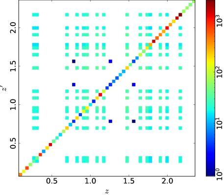
Figure 1: Figure shows the full covariance matrix of the observed Hubble parameters in the redshift interval $0.07\leq z\leq 2.36$. Colorbar represents the non-zero covariances between Hubble measurements in $\log$ scale. White pixels in the covariance plot represent redshift pairs for which covariance informations are not available.

We incorporate correlated Gaussian noises in the simulated $H(z)$ data for accounting the inherent noises of the Hubble measurements. We generate full covariance matrix corresponding to the Hubble measurements following the procedure of Moresco et al. (2020) as well as including the covariances given by Alam et al. (2017). In figure 1, we show this full covariance matrix which is used to generate the correlated Gaussian noises. We utilize the openly available code (Moresco et al., 2020) to estimate the covariances between Hubble parameters measured by Moresco et al. (2012, 2016) and Moresco (2015). Moreover, following the suggestion made by Moresco et al. (2020), we consider the bias calculations for the systematic contributions due to initial mass function (IMF) and stellar population synthesis (SPS) model (odd one out) for the estimation of the covariances corresponding to these Hubble measurements (i.e., Moresco et al. (2012, 2016); Moresco (2015)). We refer the literature (e.g., Moresco et al. (2012, 2016); Moresco (2015); Moresco et al. (2020)) for the details about the systematic contributions in the Hubble parameters measured by DA technique. For BAO $H(z)$ measurements, we use the covariances between three Hubble parameters measured by Alam et al. (2017) along with their measured variances. For the rest (Zhang et al., 2014; Jimenez et al., 2003; Simon et al., 2005; Ratsimbazafy et al., 2017; Stern et al., 2010; Gaztañaga et al., 2009; Oka et al., 2014; Wang et al., 2017; Chuang & Wang, 2013; Anderson et al., 2014; Blake et al., 2012; Busca et al., 2013; Bautista et al., 2017; Delubac et al., 2015; Font-Ribera et al., 2014) of the observed Hubble data, we utilize only corresponding variances in the diagonal of the full covariance matrix. We consider the noise distributions around $0$ mean, which are bounded by the full covariance matrix (shown in figure 1) corresponding to 53 Hubble measurements. Using random.multivariate_normal function of numpy library, we generate $1.2\times 10^{5}$ realizations of correlated Gaussian noises by using different seed values. Each of these noise realizations contains 53 values corresponding to the observed redshift points (shown in table 1). We add these correlated noises to the simulated $H(z)$ data. These noise-included realizations of $H(z)$ are used as the input of ParamANN and the corresponding values of $H_{0}$, $\Omega_{0m}$, $\Omega_{0k}$, $\Omega_{0\Lambda}$ are provided as the targets in the output layer of ParamANN.

3.4 Deep learning of ParamANN

We use open-source ML platform TensorFlow (Abadi et al., 2015), using python programming language, to create the architecture of ParamANN as well as for deep learning of this neural network.

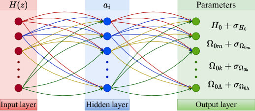
Figure 2: Figure shows the architecture of ParamANN, which contains one hidden layer in between input and output layers. Input layer contains 53 neurons representing 53 noise-included $H(z)$ values in the range $0.07\leq z\leq 2.36$, and hidden layer contains 30 neurons with ReLU activation (i.e., $\{a_{i}:i\in\{0,1,...,29\}\}$). Output layer contains 8 neurons in which first four neurons represent the predicted parameters (i.e., $H_{0}$, $\Omega_{0m}$, $\Omega_{0k}$ and $\Omega_{0\Lambda}$) and last four neurons predict the uncertainties corresponding to these parameters.

3.4.1 ParamANN

We construct ParamANN with one hidden layer for the direct mapping between noise-included H(z) and four fundamental parameters (i.e., $H_{0}$, $\Omega_{0m}$, $\Omega_{0k}$, $\Omega_{0\Lambda}$) of $\Lambda$CDM universe. In figure 2, we present the architecture of ParamANN. In ParamANN, input layer contains fifty three neurons, hidden layer consists of thirty neurons and the output layer comprises eight neurons. Neurons of each layer are densely connected (by weights and biases) to each neurons of the previous layer. We note that first half of the output layer shows the predictions and second half of the same provides the uncertainties corresponding to these predictions. To train the ParamANN, we use the noise-included $H(z)$ as input and the corresponding parameter values (i.e., $\hat{H}_{0}$, $\hat{\Omega}_{0m}$, $\hat{\Omega}_{0k}$, $\hat{\Omega}_{0\Lambda}$) are used as targets, where the ‘hat’ notation is used to define the target parameters. We use ReLU (Agarap, 2019) activation function in the hidden layer to learn the non-linearity of the direct mapping between input and targets. For the optimization process using mini-batch algorithm (Ruder, 2016; Sun et al., 2020), we utilize adaptive moment estimation (ADAM) (Kingma & Ba, 2014) optimizer with learning rate $5\times 10^{-4}$ to update weights and biases in the backward propagation (Hecht-Nielsen, 1992) of the training process of ParamANN.

3.4.2 Preprocessing of data

Preprocessing is widely known procedure to normalize the input data (generally distributing the values in the lower range) for the better performance of supervised learning of ANN. Moreover, normalized input data can speed up the training process of neural network. The familiar techniques for the preprocessing are min-max normalization, z-score normalization (i.e., standardization) etc. (Kotsiantis et al., 2007). We use the standardization method to normalize the noise-included $H(z)$ data which are used as input in ParamANN. Four fundamental parameters (i.e., $\hat{H}_{0}$, $\hat{\Omega}_{0m}$, $\hat{\Omega}_{0k}$, $\hat{\Omega}_{0\Lambda}$) corresponding to these input are used as targets without any scaling. After random shuffling of the entire data, we split these data in three sets (i.e., training, validation and test sets). We use $10^{5}$ data for training, $1.5\times 10^{4}$ data for validation and $5\times 10^{3}$ data for testing the predictions of ParamANN. To perform the standardization in input, at first we obtain mean and standard deviation of noise-included $H(z)$ data of training set. Then, each sample of these three sets is subtracted by this mean and divided by this standard deviation. We use the mean and standard deviation of training set even in the validation and test sets, which helps to pass the informations about the training of ParamANN into these data sets effectively. After normalizing the noise-included $H(z)$ of these three sets by using the standardization method, we use these standardized $H(z)$ data as normalized input in ParamANN.

3.4.3 Loss function

In our analysis, we use heteroscedastic (HS) loss function (Kendall & Gal, 2017) which is given by

$$L^{HS}=\frac{1}{2n}\sum_{q=0}^{n}\left[\exp(-s_{q})\left(y_{q}-\hat{y}_{q}\right)^{2}+s_{q}\right],$$ (13)

where $n$ defines the number of targets which is four in our analysis. In equation 13, $y_{q}$ and $\hat{y}_{q}$ represent the predictions and targets respectively. Moreover, in this equation, $s_{q}$ is the log variances (i.e., $\ln\sigma_{q}^{2}$) corresponding to the predictions, where $\sigma_{q}$ denotes the aleatoric uncertainty of prediction. Using this special type of loss function, we obtain the uncertainties (i.e., aleatoric uncertainty) corresponding to each predictions. Therefore, the output layer of ParamANN contains eight neurons, in which first four neurons estimate the values of the cosmological parameters and rest of them evaluate the uncertainties corresponding to these parameters.

This HS loss function is equivalent to the negative log-likelihood function which is commonly utilized in the traditional approaches for cosmological analysis. Similar to the usual likelihood method, ParamANN minimizes the HS loss function by comparing the predictions with targets. Therefore, the uncertainty measurements of predicted parameters provided by this loss function are equivalent to the maximum-likelihood estimates of the cosmological parameters in the case of a traditional method.

3.4.4 Training and prediction

We train ParamANN by using $10^{5}$ realizations of standardized $H(z)$ data (in the range $0.07\leq z\leq 2.36$) and corresponding target parameters (i.e., $\hat{H}_{0}$, $\hat{\Omega}_{0m}$, $\hat{\Omega}_{0k}$, $\hat{\Omega}_{0\Lambda}$). Training process continues in an iterative way by minimizing HS loss function used in the neural network. We use 100 epochs to decide how many times the optimization process should continue. Moreover, each epoch completes with a fixed number of iterations since we choose the mini-batch size of 128. Depending upon the mini-batch size, each iteration takes a subset from the entire training set to minimize the HS loss function (equation 13). Therefore, one can estimate the number of iterations in each epoch by taking the ratio between the number of training samples and the mini-batch size. In our analysis, the number of iterations in each epoch is 782. We use model averaging ensemble (MAE) method (Lai et al., 2022) to reduce the epistemic uncertainties in the predicted parameters. For MAE method, we perform the training of ParamANN 100 times (with the same data and the same tuning of hyperparameters) by varying the initialization of weights using 100 randomly selected seed values. The entire training process of these 100 ensembles takes approximately 85 minutes to execute in a Intel(R) Core(TM) i7-10700 CPU system (contains two threads in each of eight cores) with 2.9 GHz processor speed. We also use $1.5\times 10^{4}$ number of validation data at the time of training process to check any kind of overfitting or underfitting in the minimization of HS loss function and notice no overfitting or underfitting in the training of ParamANN.

After completion of the entire training process, we predict the values of parameters (i.e., $H_{0}$, $\Omega_{0m}$, $\Omega_{0k}$, $\Omega_{0\Lambda}$) with corresponding log variances by using $5\times 10^{3}$ number (i.e., test set) of standardized $H(z)$ data in 100 ensembles of trained ParamANN. We estimate the final predictions of these parameters by taking the mean of 100 ensembles of the predicted parameter values for each realization of the test set. To calculate the uncertainties corresponding to these final predictions, at first we take the exponential of the log variances to obtain the variances corresponding to 100 ensembles of these parameters for each realization of test set. Then, we estimate the mean of 100 ensembles of variances and take the square root of these averaged variances to obtain the uncertainties corresponding to the final predictions of these parameters for each realization of test set.

4 Results and analysis

In this section, at first we show the predicted results for test set. Then, we present the predictions of ParamANN for Hubble measurements (DA+BAO) and compare these predictions with the results estimated by Planck collaboration VI (2020).

4.1 Predictions for test set

We predict the Hubble constant ($H_{0}$) and the density parameters (i.e., $\Omega_{0m}$, $\Omega_{0k}$, $\Omega_{0\Lambda}$) of $\Lambda$CDM universe with their corresponding uncertainties (i.e., $\sigma_{H_{0}}$, $\sigma_{\Omega_{0m}}$, $\sigma_{\Omega_{0k}}$, $\sigma_{\Omega_{0\Lambda}}$) by using the noise-included $H(z)$ data of test set in trained ParamANN. We compare these predictions with the corresponding targets (i.e., $\hat{H}_{0}$, $\hat{\Omega}_{0m}$, $\hat{\Omega}_{0k}$, $\hat{\Omega}_{0\Lambda}$) to show the accuracy of the predictions of ParamANN. We estimate the differences between the targets and predictions of the test set by using the equation which is given by

$$\Delta_{y} = \hat{y}-y,$$ (14)

where $y$ represents the predicted parameters, i.e., $H_{0}$, $\Omega_{0m}$, $\Omega_{0k}$, $\Omega_{0\Lambda}$, and $\hat{y}$ defines the corresponding target parameters, i.e., $\hat{H}_{0}$, $\hat{\Omega}_{0m}$, $\hat{\Omega}_{0k}$, $\hat{\Omega}_{0\Lambda}$.

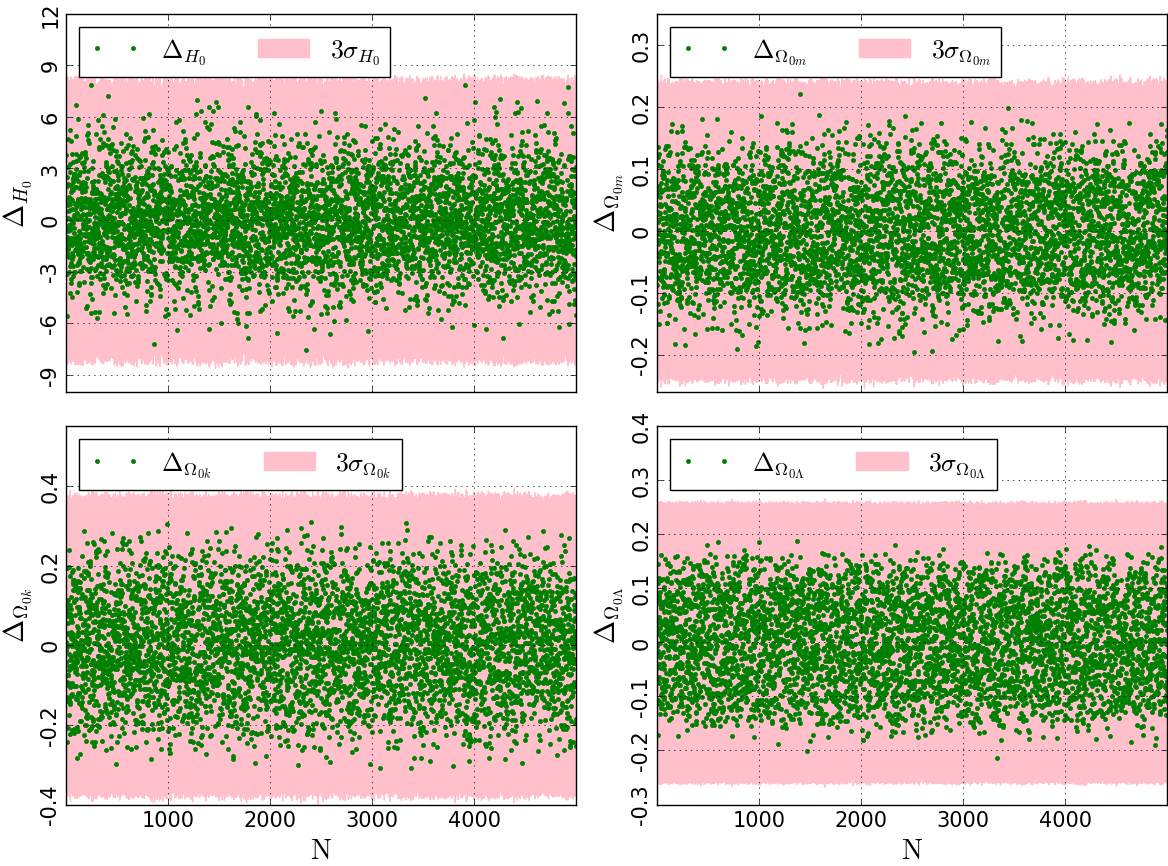
Figure 3: Top left subfigure shows the differences between target and predicted Hubble constant. In top right subfigure, we show the differences between target and predicted matter density. Similarly, in bottom left and bottom right subfigures, we present the differences between target and prediction for curvature and vacuum density parameters respectively. Moreover, in each of these subfigures, we show three times uncertainties of the corresponding predictions. Horizontal axis of each subfigure represents the index number of test samples.

In the top left subfigure of figure 3, we present the differences between target and predictions for Hubble constant. In the same figure, we show the similar differences for matter, curvature and vacuum density parameters in top right, bottom left and bottom right subfigures respectively. In each of these subfigures of figure 3, we also present three times predicted uncertainties of the corresponding predicted parameters for test set. We note that the differences corresponding to each of these parameters dominantly lie within their three times uncertainty ranges. Therefore, we conclude that the predictions of test set agree well with the corresponding targets within the corresponding predicted uncertainties.

4.2 Predictions for Hubble measurements

We train the ParamANN by using mock $H(z)$ values (for the range $0.07\leq z\leq 2.36$) as input. Moreover, these mock $H(z)$ values contain the correlated noises compatible with observed Hubble parameters. Therefore, we can use the observed $H(z)$ values (shown in table 1) directly to the trained ParamANN (after performing the standardization method) to extract the values of Hubble constant, matter, curvature, and vacuum density parameters with their corresponding uncertainties for the present $\Lambda$CDM universe.

4.2.1 Hubble constant and density parameters

In table 2, we show the present values of Hubble parameter ($H_{0}$) and three density parameters (i.e., $\Omega_{0m}$, $\Omega_{0k}$, $\Omega_{0\Lambda}$) with their corresponding uncertainties which are estimated from the trained ParamANN by using the observed Hubble data (DA+BAO). We compare our estimated values of these four parameters with the values of these same parameters obtained by Planck collaboration VI (2020).

Table 2: Table shows the values of Hubble constant ($H_{0}$ in $\rm{kmMpc^{-1}sec^{-1}}$) and three density parameters (i.e., $\Omega_{0m}$, $\Omega_{0k}$, $\Omega_{0\Lambda}$) predicted by ParamANN from the observed $H(z)$ parameter values. Third column of this table represents the significance of these predictions with respect to the results (shown in table 3) obtained by Planck collaboration VI (2020).

Parameter	Value	Significance
$H_{0}$	$66.11\pm 2.59$	$0.6\sigma$
$\Omega_{0m}$	$0.3359\pm 0.0814$	$0.3\sigma$
$\Omega_{0k}$	$0.0237\pm 0.1248$	$0.18\sigma$
$\Omega_{0\Lambda}$	$0.6405\pm 0.0861$	$0.56\sigma$

Table 3: Table shows the values of Hubble constant ($H_{0}$ in $\rm{kmMpc^{-1}sec^{-1}}$), matter ($\Omega_{0m}$), curvature ($\Omega_{0k}$) and vacuum ($\Omega_{0\Lambda}$) density parameters estimated by Planck collaboration VI (2020).

Parameter	Value
$H_{0}$	$67.66\pm 0.42$
$\Omega_{0m}$	$0.3111\pm 0.0056$
$\Omega_{0k}$	$0.001\pm 0.002$
$\Omega_{0\Lambda}$	$0.6889\pm 0.0056$

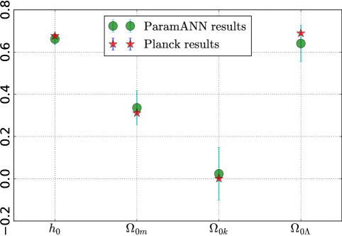
Figure 4: Figure represents the values of parameters (i.e., $h_{0}$, $\Omega_{0m}$, $\Omega_{0k}$, $\Omega_{0\Lambda}$) with corresponding error bars obtained by ParamANN as well as estimated by Planck collaboration VI (2020). The Hubble constant ($h_{0}$) is represented in the unit of 100 $\rm{kmMpc^{-1}sec^{-1}}$. Horizontal axis indicates these four parameters and vertical axis represents the values of these parameters.

In table 3, we show the values of these cosmological parameters constrained by Planck collaboration VI (2020) for $\Lambda$CDM universe. We note that the predicted uncertainties corresponding to our estimated parameters are comparably larger than the uncertainties of Planck’s estimated values of these parameters, since the observed Hubble data are lesser numbers than CMB data as well as these $H(z)$ data (specifically DA data) contain larger uncertainties including various systematic effects. We calculate the significances of the parameter values, predicted by ParamANN, with respect to the Planck’s results. We estimate these significances by taking the absolute differences between our estimated parameters and Planck’s results as well as dividing these absolute differences by the corresponding uncertainties predicted by ParamANN. We show these significances in the third column of table 2, where $\sigma$ denotes the uncertainties (predicted by ParamANN) corresponding to the parameters. We notice that our estimation of $H_{0}$ from observed Hubble data shows less deviation (i.e., $0.6\sigma$) from the value of $H_{0}$ obtained by Planck collaboration VI (2020). Less deviation of our estimated $H_{0}$ from Planck’s $H_{0}$ value indicates the alleviation of so-called Hubble tension by using observed Hubble data (DA+BAO) alone. Moreover, matter ($\Omega_{0m}$), curvature ($\Omega_{0k}$) and vacuum ($\Omega_{0\Lambda}$) densities predicted by the ParamANN show less deviations (i.e., $0.3\sigma$, $0.18\sigma$ and $0.56\sigma$ respectively) from the values of these parameters constrained by Planck collaboration VI (2020). These low significances (shown in table 2) corresponding to our estimated parameters indicate the better agreement between ours and Planck’s estimates of these four cosmological parameters (i.e., $H_{0}$, $\Omega_{0m}$, $\Omega_{0k}$, $\Omega_{0\Lambda}$). We note that, although the ParamANN is trained for generalized $\Lambda$CDM universe by considering spatial curvature density, this trained ParamANN predict spatially flat $\Lambda$CDM universe and alleviates the so-called Hubble tension by using Hubble measurements (DA+BAO) alone. In figure 4, we demonstrate the estimated values of Hubble constant ($h_{0}$) and three density parameters (i.e., $\Omega_{0m}$, $\Omega_{0k}$, $\Omega_{0\Lambda}$) provided by trained ParamANN as well as the values of these parameters constrained by Planck collaboration VI (2020). In this same figure, we also show the uncertainties corresponding to these parameters. We note that in this figure we present the Hubble constant in unit 100 $\rm{kmMpc^{-1}sec^{-1}}$.

4.2.2 Hubble parameter curve

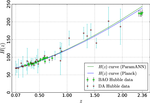
Figure 5: Figure shows the Hubble parameter curve computed by using our estimated parameters in green color and the same is determined by using the Planck’s parameter values in blue color. In the same figure, we also present the Hubble parameters measured by DA and BAO techniques. In this figure, the horizontal axis represents the redshifts and the vertical axis defines the values of the Hubble parameter (in $\rm{kmMpc^{-1}sec^{-1}}$ unit) at these redshifts.

We obtain the Hubble parameter curve (equation 10) using the parameter values (shown in table 2) predicted by trained ParamANN. We also compute the same by using the parameter values (shown in table 3) constrained by Planck collaboration VI (2020). In figure 5, we show these two curves along with the data points (in the range $0.07\leq z\leq 2.36$) measured by DA and BAO techniques. Visually both the curves seem to fit the observations well. To test how these curves fit the observed points, we estimate the reduced-$\chi^{2}$ statistics as defined follow,

$$\textrm{reduced-}\chi^{2} = \frac{1}{dof}\sum_{i,j=0}^{52}\left[H(z_{i})-H_{obs}(z_{i})\right]\left[C^{-1}\right]_{ij}\left[H(z_{j})-H_{obs}(z_{j})\right],$$ (15)

where $i,j$ are the dummy indices and ‘dof’ indicates the number of degrees of freedom, which is 50 in this case since we use 53 Hubble data to estimate three independent parameters. In equation 15, $H_{obs}(z)$ defines 53 observed Hubble data (shown in table 1), $H(z)$ represents the Hubble parameters estimated by using our predicted parameters (or Planck’s results) at observed redshift points, and $C$ denotes the covariance matrix shown in figure 1. The reduced-$\chi^{2}$ value for our analysis is $\sim 0.96$. A similar value (i.e., $\sim 0.78$) was calculated for Planck curve as well. This shows that the predicted parameters by ParamANN fit the observations well. Further improvements of the error bars of the predicted parameters can be achieved once $H(z)$ observations of lower errors become available.

5 Discussions and Conclusions

Recent CMB observations indicate that our universe follows the flat $\Lambda$CDM model dominated by vacuum density (Planck collaboration VI, 2020). This vacuum density (i.e., the simplest form of dark energy) perhaps accelerates the expansion of our universe (Riess et al., 1998; Perlmutter et al., 1999). The expansion rate of the present universe can be measured by estimating the value of Hubble constant ($H_{0}$). Estimation of $H_{0}$ from the CMB observations shows a significant tension, i.e. so-called Hubble tension (Planck collaboration VI, 2020; Riess et al., 2018, 2019; Riess, 2020; Riess et al., 2021, 2022; Wong et al., 2019; Di Valentino, 2021; de Jaeger et al., 2022; Brout et al., 2022), with the value of today’s Hubble parameter constrained by local observational data (e.g., Supernovae type Ia measurements).

In this article, we predict the value of Hubble constant by employing ML algorithm using local measurements (DA+BAO) of Hubble parameter alone. We also measure the cosmological density parameters (i.e., $\Omega_{0m}$, $\Omega_{0k}$, $\Omega_{0\Lambda}$) of $\Lambda$CDM model without assuming the spatially flat curvature of our present universe. Several earlier literature constrain the cosmological parameters under the assumption of a spatially flat universe (Macaulay et al., 2013; Raveri, 2016; Shafieloo et al., 2012; Sahni et al., 2014; Zheng et al., 2016; Linder, 2003; Shahalam et al., 2015; Leaf & Melia, 2017; Geng et al., 2018; Gómez-Valent & Amendola, 2018; Bengaly et al., 2023; Liu et al., 2019; Arjona & Nesseris, 2020; Mukherjee et al., 2022; Garcia et al., 2023). However, the work of this article estimates all relevant cosmological parameters without assuming the spatial flatness of the universe. This work, therefore, provides the generalized investigations of observational data to extract the fundamental informations of our universe. Very interestingly, our measured $H_{0}$ value is in sharp agreement with the Planck collaboration VI (2020). Hence we do not see any evidences of Hubble tension using $H(z)$ data alone. Since these values are in contradiction with the $H_{0}$ value measured by Supernovae data (Riess et al., 2022) and other local measurements of $H_{0}$, further attention may be needed in future article to investigate the nature and the cause of the origin of this tension.

In a classical fitting-the-paremeter approaches (e.g., using a likelihood function), the analyses are performed by estimating the likelihood function of some distribution of observational data as well as initially providing the prior values of all or some of the parameters. The ML approach used by us can be treated as an complementary approach to these and therefore provides a mechanism to test for robustness of the scientific results with respect to various methods of analysis. The ML approaches uncover the direct mapping between input and targets to learn the hidden pattern between them. Therefore, ML can be used to learn the complex function to extract the cosmological parameters from observational data (without even assuming the Gaussian model of the noise). We therefore do not need to use any prior values of the parameters to estimate others. Given the complementarity of ML and maximum-likelihood approach, we note that our estimates of the cosmological parameters possess the properties of maximum-likelihood estimates as well (equation 13).

We create an ANN with one hidden layer containing 30 neurons. We call this ANN by a suitable name of ParamANN. We significantly train the ParamANN using $10^{5}$ samples of mock $H(z)$ values (which contain correlated noises convenient for observed Hubble data) as input and corresponding parameters as targets which are varied uniformly in their specified ranges (i.e.,$\{60,80\}$ $\rm{kmMpc^{-1}sec^{-1}}$, $\{0.2,0.5\}$ and $\{0.5,0.8\}$ for $H_{0}$, $\Omega_{0m}$ and $\Omega_{0\Lambda}$ respectively). We note that the mock values of $\Omega_{0k}$ is calculated by $1-\Omega_{0m}-\Omega_{0\Lambda}$. We use another $1.5\times 10^{4}$ samples of mock data to validate the training of ParamANN and $5\times 10^{3}$ samples to test the performance of trained ParamANN. We note that the differences between targets and predictions for each parameter dominantly lie within three times uncertainties (predicted by ParamANN) corresponding to the predictions of test set. These results (shown in figure 3) of test set show the excellent agreement between targets and predictions of ParamANN (at least within the predicted uncertainties). Finally, we use the trained ParamANN for the predictions of the Hubble constant and the density parameters from the Hubble parameters measured by DA and BAO techniques in the redshift interval $0.07\leq z\leq 2.36$. We obtain $H_{0}=66.11\pm 2.59$ $\rm{kmMpc^{-1}sec^{-1}}$, $\Omega_{0m}=0.3359\pm 0.0814$, $\Omega_{0k}=0.0237\pm 0.1248$ and $\Omega_{0\Lambda}=0.6405\pm 0.0861$. We note that the predicted density parameters show $0.3\sigma$, $0.18\sigma$ and $0.56\sigma$ deviations from Planck’s results for matter, curvature and vacuum respectively. Moreover, our predicted Hubble constant (showing $0.6\sigma$ deviation from Planck’s result) agrees well with Planck’s estimation of $H_{0}$, which indicates the alleviation of the so-called Hubble tension by employing our ML technique.

The current article presents the first attempt to measure the four fundamental parameters (i.e., $H_{0}$, $\Omega_{0m}$, $\Omega_{0k}$, $\Omega_{0\Lambda}$) of $\Lambda$CDM universe from the Hubble measurements (DA+BAO) by using ML algorithm. In this current analysis, we consider spatially non-flat $\Lambda$CDM model to train the ParamANN for the estimates of cosmological density parameters along with Hubble constant. In a future article, we will employ the ML procedure on the different types of dark energy model (i.e., wCDM, CPL, scalar field etc.) regarding the estimations of fundamental cosmological parameters to compare these dark energy models each other.

References

- (1)
- Abadi et al. (2015) Abadi M. et al., TensorFlow: Large-Scale Machine Learning on Heterogeneous Systems, 2015, download.tensorflow.org/paper/whitepaper2015.pdf
- Agarap (2019) Agarap A. F., Deep Learning using Rectified Linear Units (ReLU), 2019, arXiv:1803.08375
- Alam et al. (2017) Alam S. et al., The clustering of galaxies in the completed SDSS-III Baryon Oscillation Spectroscopic Survey: cosmological analysis of the DR12 galaxy sample, 2017, MNRAS, 470, 2617
- Anderson et al. (2014) Anderson L., Aubourg E. et al., The clustering of galaxies in the SDSS-III Baryon Oscillation Spectroscopic Survey: measuring DA and H at from the baryon acoustic peak in the Data Release 9 spectroscopic Galaxy sample, 2014, MNRAS, 439, 83
- Zwicky (2017) Andernach H. and Zwicky F., English and Spanish Translation of Zwicky’s (1933) The Redshift of Extragalactic Nebulae, 2017, arXiv:1711.01693
- Arjona & Nesseris (2020) Arjona R. and Nesseris S., What can machine learning tell us about the background expansion of the Universe?, 2020, Phys. Rev. D, 101, 123525
- Baccigalupi et al. (2000) Baccigalupi C., Bedini L., Burigana C., de Zotti G., Farusi A., Maino D., Maris M., Perrotta F., Salerno E., Toffolatti L. and Tonazzini A., Neural networks and the separation of cosmic microwave background and astrophysical signals in sky maps, 2000, MNRAS, 318, 769
- Bautista et al. (2017) Bautista J. E., Busca N. G. et al., Measurement of baryon acoustic oscillation correlations at with SDSS DR12 Ly-Forests, 2017, A&A, 603, A12
- Bengaly et al. (2023) Bengaly C., Dantas M. A., Casarini L. and Alcaniz J., Measuring the Hubble constant with cosmic chronometers: a machine learning approach, 2023, The European Physical Journal C, 83, 548
- Blake & Glazebrook (2003) Blake C. and Glazebrook K., Probing Dark Energy Using Baryonic Oscillations in the Galaxy Power Spectrum as a Cosmological Ruler, 2003, ApJ, 594, 665
- Blake et al. (2012) Blake C., Brough S., Colless M. et al., The WiggleZ Dark Energy Survey: joint measurements of the expansion and growth history at , 2012, MNRAS, 425, 405
- Brout et al. (2022) Brout D. et al., The Pantheon+ Analysis: Cosmological Constraints, 2022, ApJ, 938, 110
- Busca et al. (2013) Busca N. G., Delubac T., Rich J., Bailey S., Font-Ribera A. et al., Baryon acoustic oscillations in the Ly forest of BOSS quasars, 2013, A&A, 552, A96
- Cao et al. (2021) Cao S., Ryan J. and Ratra B., Using Pantheon and DES supernova, baryon acoustic oscillation, and Hubble parameter data to constrain the Hubble constant, dark energy dynamics, and spatial curvature, 2021, MNRAS, 504, 300
- Cao & Ratra (2022) Cao S. and Ratra B., Using lower redshift, non-CMB, data to constrain the Hubble constant and other cosmological parameters, 2022, MNRAS, 513, 5686
- Chanda & Saha (2021) Chanda P. and Saha R., An unbiased estimator of the full-sky CMB angular power spectrum at large scales using neural networks, 2021, MNRAS, 508, 4600
- Chevalier & Polarski (2001) Chevalier M. & Polarski D., ACCELERATING UNIVERSES WITH SCALING DARK MATTER, 2001, IJMPD, 10, 213
- Chuang & Wang (2013) Chuang C. H. & Wang Y., Modelling the anisotropic two-point galaxy correlation function on small scales and single-probe measurements of H(z), and f(z) from the Sloan Digital Sky Survey DR7 luminous red galaxies, 2013, MNRAS, 435, 255
- de Jaeger et al. (2022) de Jaeger T. et al., A 5 per cent measurement of the Hubble-Lemaitre constant from Type II supernovae, 2022, MNRAS, 514, 4620
- Delubac et al. (2015) Delubac T. et al., Baryon acoustic oscillations in the Ly forest of BOSS DR11 quasars, 2015, A&A, 574, A59
- Dewdney et al. (2009) Dewdney P. E., Hall P. J., Schilizzi R. T. and Lazio T. J. L. W., The Square Kilometre Array, 2009, Proceedings of the IEEE, 97, 1482
- Dialektopoulos et al. (2022) Dialektopoulos K., Said J. L., Mifsud J., Sultana J. and Adami K. Z., Neural network reconstruction of late-time cosmology and null tests, 2022, JCAP, 2022, 023
- Di Valentino (2021) Di Valentino E., A combined analysis of the late time direct measurements and the impact on the Dark Energy sector, 2021, MNRAS, 502, 2065
- Albert Einstein (1917) Einstein, A., Sitz. Preuss. Akad. d. Wiss. Phys.-Math 142 (1917).
- Escamilla-Rivera et al. (2020) Escamilla-Rivera C., Quintero M. A. C. and Capozziello S., A deep learning approach to cosmological dark energy models, 2020, JCAP, 2020, 008
- Font-Ribera et al. (2014) Font-Ribera A., Kirkby D., Busca N.G. et al., Quasar-Lyman forest cross-correlation from BOSS DR11: Baryon Acoustic Oscillations, 2014, JCAP, 05, 027
- Freedman (2021) Freedman W. L., Measurements of the Hubble Constant: Tensions in Perspective*, 2021, ApJ, 919, 16
- Freeman (1970) Freeman, K. C., On the Disks of Spiral and S0 Galaxies, 1970, ApJ, 160, 811
- Garcia et al. (2023) Garcia C., Santa C. and Romano A. E., Deep learning reconstruction of the large-scale structure of the Universe from luminosity distance, 2023, MNRAS, 518, 2241
- Gaztañaga et al. (2009) Gaztañaga E., Cabré A. & Hui L., Clustering of luminous red galaxies-IV. Baryon acoustic peak in the line-of-sight direction and a direct measurement of H(z), 2009, MNRAS, 399, 1663
- Geng et al. (2018) Geng J. J., Guo R. Y., Wang A. Z., Zhang J. F. and Zhang X., Prospect for Cosmological Parameter Estimation Using Future Hubble Parameter Measurements, 2018, Communications in Theoretical Physics, 70, 445
- Gómez-Valent & Amendola (2018) Gómez-Valent A. and Amendola L., from cosmic chronometers and Type Ia supernovae, with Gaussian Processes and the novel Weighted Polynomial Regression method, 2018, JCAP, 04, 051
- Gómez-Vargas et al. (2021) Gómez-Vargas I., Esquivel R. M., Garcia-Salcedo R. and Vázquez J. A., Neural network within a Bayesian inference framework, 2021, Journal of Physics: Conference Series, 1723, 012022
- Gómez-Vargas et al. (2023) Gómez-Vargas I., Vázquez J. A., Esquivel R. M. and Garcia-Salcedo R., Neural network reconstructions for the Hubble parameter, growth rate and distance modulus, 2023, The European Physical Journal C, 83, 304
- Graff et al. (2012) Graff P., Feroz F., Hobson M. P. and Lasenby A., BAMBI: blind accelerated multimodal Bayesian inference, 2012, MNRAS, 421, 169
- Hanany et al. (2019) Hanany, S. et al., PICO: Probe of Inflation and Cosmic Origins, 2019, arXiv:1902.10541
- Hazumi et al. (2020) Hazumi, M. et al., LiteBIRD satellite: JAXA’s new strategic L-class mission for all-sky surveys of cosmic microwave background polarization, 2020, International Society for Optics and Photonics, 11443, 114432F
- Hecht-Nielsen (1992) Hecht-Nielsen R., in Neural Networks for Perception., 1992, Academic Press, pp 65–93, doi.org/10.1016/B978-0-12-741252-8.50010-8
- Hortua et al. (2020) Hortua H. J., Volpi R., Marinelli D. and Malago L., Accelerating MCMC algorithms through Bayesian Deep Networks, 2020, arXiv:2011.14276
- Jimenez & Loeb (2002) Jimenez R. & Loeb A., Constraining Cosmological Parameters Based on Relative Galaxy Ages, 2002, ApJ, 573, 37
- Jimenez et al. (2003) Jimenez R., Verde L., Treu T., & Stern D., Constraints on the Equation of State of Dark Energy and the Hubble Constant from Stellar Ages and the Cosmic Microwave Background, 2003, ApJ, 593, 622
- Kelly et al. (2023) Kelly P. L. et al., Constraints on the Hubble constant from supernova Refsdal’s reappearance, 2023, Science, 380, eabh1322
- Kendall & Gal (2017) Kendall A., Gal Y., What Uncertainties Do We Need in Bayesian Deep Learning for Computer Vision?, 2017, arXiv:1703.04977
- Khan & Saha (2023) Khan, M. I. and Saha, R., Detection of Dipole Modulation in CMB Temperature Anisotropy Maps from WMAP and Planck using Artificial Intelligence, 2023, ApJ, 947, 47
- Kingma & Ba (2014) Kingma D. P., Ba J., Adam: A method for stochastic optimization, 2014, arXiv:1412.6980
- Kotsiantis et al. (2007) Kotsiantis S. B., Kanellopoulos D. and Pintelas P. E., Data Preprocessing for Supervised Leaning, 2007, International Journal of Computer and Information Engineering, 1, 4104
- Lacki & Beacom (2010) Lacki B. C. and Beacom J. F., PRIMORDIAL BLACK HOLES AS DARK MATTER: ALMOST ALL OR ALMOST NOTHING, 2010, ApJL, 720, L67
- Lai et al. (2022) Lai Y., Shi Y., Han Y., Shao Y., Qi M. and Li B., Exploring uncertainty in regression neural networks for construction of prediction intervals, 2022, Neurocomputing, 481, 249
- Leaf & Melia (2017) Leaf, K. and Melia, F., Analysing H(z) data using two-point diagnostics, 2017, MNRAS, 470, 2320
- Linder (2003) Linder E. V., Exploring the Expansion History of the Universe, 2003, Phys. Rev. Lett., 90, 091301
- Liu et al. (2019) Liu T., Cao S., Zhang J., Geng S., Liu Y., Ji X. and Zhu Z. H., Implications from Simulated Strong Gravitational Lensing Systems: Constraining Cosmological Parameters Using Gaussian Processes, 2019, ApJ, 886, 94
- Liu et al. (2021) Liu T., Cao S., Zhang S., Gong X., Guo W. and Zheng C., Revisiting the cosmic distance duality relation with machine learning reconstruction methods: the combination of HII galaxies and ultra-compact radio quasars, 2021, The European Physical Journal C, 81, 903
- Macaulay et al. (2013) Macaulay, E., Wehus, I. K. and Eriksen, H. K., Lower Growth Rate from Recent Redshift Space Distortion Measurements than Expected from Planck, 2013, Phys. Rev. Lett., 111, 161301
- Mancini et al. (2022) Mancini A. S., Piras D., Alsing J., Joachimi B. and Hobson M. P., CosmoPower: emulating cosmological power spectra for accelerated Bayesian inference from next-generation surveys, 2022, MNRAS, 511, 1771
- Moresco et al. (2012) Moresco M., Cimatti A., Jimenez R. et al., Improved constraints on the expansion rate of the Universe up to from the spectroscopic evolution of cosmic chronometers, 2012, JCAP, 08, 006
- Moresco (2015) Moresco M., Raising the bar: new constraints on the Hubble parameter with cosmic chronometers at , 2015, MNRAS, 450, L16
- Moresco et al. (2016) Moresco M., Pozzetti L., Cimatti A. et al., A 6% measurement of the Hubble parameter at : direct evidence of the epoch of cosmic re-acceleration, 2016, JCAP, 05, 014
- Moresco et al. (2020) Moresco M., Jimenez R., Verde L., Cimatti A. and Pozzetti L., Setting the Stage for Cosmic Chronometers. II. Impact of Stellar Population Synthesis Models Systematics and Full Covariance Matrix, 2020, ApJ, 898, 82
- Moss (2020) Moss A., Accelerated Bayesian inference using deep learning, 2020, MNRAS, 496, 328
- Mukherjee et al. (2022) Mukherjee P., Said J. L. and Mifsud J., Neural network reconstruction of and its application in teleparallel gravity, 2022, JCAP, 2022, 029
- Mukherjee et al. (2020) Mukherjee S. et al., First measurement of the Hubble parameter from bright binary black hole GW190521, 2020, arXiv:2009.14199
- Oka et al. (2014) Oka A., Saito S., Nishimichi T., Taruya A. & Yamamoto K., Simultaneous constraints on the growth of structure and cosmic expansion from the multipole power spectra of the SDSS DR7 LRG sample, 2014, MNRAS, 439, 2515
- Olvera et al. (2022) Olvera J. de D. R., Gómez-Vargas I. and Vázquez J. A., Observational cosmology with Artificial Neural Networks, 2022, Universe, 8, 120
- Pal et al. (2023) Pal S., Chanda P. and Saha R., Estimation of the Full-sky Power Spectrum between Intermediate and Large Angular Scales from Partial-sky CMB Anisotropies Using an Artificial Neural Network, 2023, ApJ, 945, 77
- Pal & Saha (2023) Pal S. and Saha R., Reconstruction of full sky CMB E and B modes spectra removing E-to-B leakage from partial sky using deep learning, 2023, arXiv:2211.09112
- Perlmutter et al. (1999) Perlmutter, S., Aldering, G. et al., Measurements of and from 42 High-Redshift Supernovae, 1999, ApJ, 517, 565
- Petroff et al. (2020) Petroff M. A., Addison G. E., Bennett C. L., Weiland J. L., Full-sky Cosmic Microwave Background Foreground Cleaning Using Machine Learning, 2020, ApJ, 903, 104
- Planck collaboration VI (2020) Planck Collaboration VI., Planck 2018 results VI. Cosmological parameters, 2020, A&A, 641, A6
- Ratsimbazafy et al. (2017) Ratsimbazafy A. L. et al., Age-dating luminous red galaxies observed with the Southern African Large Telescope, 2017, MNRAS, 467, 3239
- Raveri (2016) Raveri M., Are cosmological data sets consistent with each other within the cold dark matter model?, 2016, Phys. Rev. D, 93, 043522
- Riess et al. (1998) Riess, A. G., Filippenko, A. V. et al., Observational Evidence from Supernovae for an Accelerating Universe and a Cosmological Constant, 1998, AJ, 116, 1009
- Riess et al. (2018) Riess A. G., Casertano S., Yuan W. et al., New Parallaxes of Galactic Cepheids from Spatially Scanning the Hubble Space Telescope: Implications for the Hubble Constant, 2018, ApJ, 855, 136
- Riess et al. (2019) Riess A. G., Casertano S., Yuan W. et al., Large Magellanic Cloud Cepheid Standards Provide a 1% Foundation for the Determination of the Hubble Constant and Stronger Evidence for Physics beyond CDM, 2019, ApJ, 876, 85
- Riess (2020) Riess A. G., The expansion of the Universe is faster than expected, 2020, Nat. Rev. Phys., 2, 10
- Riess et al. (2021) Riess A. G., Casertano S., Yuan W. et al., Cosmic Distances Calibrated to 1% Precision with Gaia EDR3 Parallaxes and Hubble Space Telescope Photometry of 75 Milky Way Cepheids Confirm Tension with CDM, 2021, ApJL, 908, L6
- Riess et al. (2022) Riess A. G., Yuan W., Macri L. M. et al., A Comprehensive Measurement of the Local Value of the Hubble Constant with 1 Uncertainty from the Hubble Space Telescope and the SH0ES Team, 2022, ApJL, 934, L7
- Ruder (2016) Ruder S., An overview of gradient descent optimization algorithms, 2016, arXiv:1609.04747
- Ryan et al. (2018) Ryan J., Doshi S. and Ratra B., Constraints on dark energy dynamics and spatial curvature from Hubble parameter and baryon acoustic oscillation data, 2018, MNRAS, 480, 759
- Ryan et al. (2019) Ryan J., Chen Y. and Ratra B., Baryon acoustic oscillation, Hubble parameter, and angular size measurement constraints on the Hubble constant, dark energy dynamics, and spatial curvature, 2019, MNRAS, 488, 3844
- Sahni et al. (2008) Sahni V., Shafieloo A., & Starobinsky A. A., Two new diagnostics of dark energy, 2008, Phys. Rev. D, 78, 103502
- Sahni et al. (2014) Sahni V., Shafieloo A., & Starobinsky A. A., MODEL-INDEPENDENT EVIDENCE FOR DARK ENERGY EVOLUTION FROM BARYON ACOUSTIC OSCILLATIONS, 2014, ApJL, 793, L40
- Seo & Eisenstein (2003) Seo H. and Eisenstein D. J., Probing Dark Energy with Baryonic Acoustic Oscillations from Future Large Galaxy Redshift Surveys, 2003, ApJ, 598, 720
- Shafieloo et al. (2012) Shafieloo A., Sahni V., & Starobinsky A. A., New null diagnostic customized for reconstructing the properties of dark energy from baryon acoustic oscillations data, 2012, Phys. Rev. D, 86, 103527
- Shahalam et al. (2015) Shahalam M., Sami S. and Agarwal A., Om diagnostic applied to scalar field models and slowing down of cosmic acceleration, 2015, MNRAS, 448, 2948
- Shallue & Eisenstein (2023) Shallue C. J. and Eisenstein D. J., Reconstructing cosmological initial conditions from late-time structure with convolutional neural networks, 2023, MNRAS, 520, 6256
- Simon et al. (2005) Simon J., Verde L., & Jimenez R., Constraints on the redshift dependence of the dark energy potential, 2005, Phys. Rev. D, 71, 123001
- Stacey et al. (2018) Stacey J. G. et al., CCAT-Prime: science with an ultra-widefield submillimeter observatory on Cerro Chajnantor, 2018, International Society for Optics and Photonics, 10700, 482
- Stern et al. (2010) Stern D., Jimenez R., Verde L. et al., Cosmic chronometers: constraining the equation of state of dark energy. I: H(z) measurements, 2010, JCAP, 02, 008
- Sun et al. (2020) Sun S., Cao Z., Zhu H., Zhao J., A Survey of Optimization Methods From a Machine Learning Perspective, 2020, IEEE Transactions on Cybernetics, 50, 3668
- Uzan et al. (2008) Uzan J. P., Clarkson C. and Ellis G. F. R., Time Drift of Cosmological Redshifts as a Test of the Copernican Principle, 2008, Phys. Rev. Lett., 100, 191303
- Valkenburg et al. (2014) Valkenburg W., Marra V. and Clarkson C., Testing the Copernican principle by constraining spatial homogeneity, 2014, MNRAS, 438, L6
- Wang et al. (2017) Wang Y. et al., The clustering of galaxies in the completed SDSS-III Baryon Oscillation Spectroscopic Survey: tomographic BAO analysis of DR12 combined sample in configuration space, 2017, MNRAS, 469, 3762
- Wang et al. (2020a) Wang G. J., Ma X. J., Li S. Y. and Xia J. Q., Reconstructing Functions and Estimating Parameters with Artificial Neural Networks: A Test with a Hubble Parameter and SNe Ia, 2020, ApJS, 246, 13
- Wang et al. (2020b) Wang G. J., Li S. Y. and Xia J. Q., ECoPANN: A Framework for Estimating Cosmological Parameters Using Artificial Neural Networks, 2020, ApJS, 249, 25
- Wang et al. (2021) Wang Y. C., Xie Y. B., Zhang T. J., Huang H. C., Zhang T. and Liu K., Likelihood-free Cosmological Constraints with Artificial Neural Networks: An Application on Hubble Parameters and SNe Ia, 2021, ApJS, 254, 43
- Wong et al. (2019) Wong K. C., Suyu S. H., Chen G. C. F. et al., H0LiCOW – XIII. A 2.4 per cent measurement of from lensed quasars: 5.3 tension between early- and late-Universe probes, 2019, MNRAS, 498, 1420
- Zhang et al. (2014) Zhang C., Zhang H., Yuan S. et al., Four new observational data from luminous red galaxies in the Sloan Digital Sky Survey data release seven, 2014, Res. Astron. Astrophys., 14, 1221
- Zheng et al. (2016) Zheng X., Ding X., Biesiada M., Cao S. & Zhu Z. H., WHAT ARE THE AND DIAGNOSTICS TELLING US IN LIGHT OF DATA?, 2016, ApJL, 825, 17
- Zunckel & Clarkson (2008) Zunckel C., Clarkson C., Consistency Tests for the Cosmological Constant, 2008, Phys. Rev. Lett., 101, 181301