Conservative World Models

Abstract

Zero-shot reinforcement learning (RL) promises to provide agents that can perform any task in an environment after an offline pre-training phase. Forward-backward (FB) representations represent remarkable progress towards this ideal, achieving 85% of the performance of task-specific agents in this setting. However, such performance is contingent on access to large and diverse datasets for pre-training, which cannot be expected for most real problems. Here, we explore how FB performance degrades when trained on small datasets that lack diversity, and mitigate it with conservatism, a well-established feature of performant offline RL algorithms. We evaluate our family of methods across various datasets, domains and tasks, reaching 150% of vanilla FB performance in aggregate. Somewhat surprisingly, conservative FB algorithms also outperform the task-specific baseline, despite lacking access to reward labels and being required to maintain policies for all tasks. Conservative FB algorithms perform no worse than FB on full datasets, and so present little downside over their predecessor. Our code is available open-source via https://enjeeneer.io/projects/conservative-world-models/.

1 Introduction

Humans construct internal models of the world to solve varied tasks efficiently. Much work has focused on equipping artificial agents with analogous models (Sutton, 1991; Deisenroth & Rasmussen, 2011; Chua et al., 2018; Ha & Schmidhuber, 2018; Hafner et al., 2019; Schrittwieser et al., 2020; Hafner et al., 2023), but in most cases these agents have lacked the adaptability of humans. However, some agents, like those utilising successor features (Barreto et al., 2017; Borsa et al., 2018) and forward-backward (FB) representations (Touati & Ollivier, 2021; Touati et al., 2022), can solve any task in an environment with no online planning or learning, and so appear to exhibit the adaptability we desire. They achieve this by learning a model that predicts the agent’s future state visitations when attempting to solve unencountered tasks, building a family of policies for these tasks given the model’s predictions, and then selecting the correct policy when a test task is specified. It is models that can be used to achieve this generality that we call world models.

Recent attention has been paid to training world models on offline data, a setting known as zero-shot reinforcement learning (RL) (Kirk et al., 2023). The appeal of zero-shot RL is in providing agents that can solve any task in an environment without the need for dangerous or expensive online interaction. In Touati et al. (2022), FB models pre-trained on datasets of reward-free transitions are able to return policies for unseen tasks in an environment that are 85% as performant as those returned by offline RL algorithms explicitly trained for each task. FB achieves this with no prior knowledge of the tasks, zero planning, and no online interaction. FB thus represents remarkable progress towards the ideal of zero-shot RL.

However, such performance is only achievable if the pre-training dataset is large and diverse. Real datasets, like those produced by an existing controller or collected by a task-directed agent, are usually small and lack diversity. Even if we design agents to exhaustively explore environments, as is done in Unsupervised RL (Jaderberg et al., 2016), they suffer the impracticalities of the online RL algorithms we are trying to avoid: they act dangerously in safety-critical environments, and data collection is time-consuming.

Is it possible to relax the requirement for large and diverse datasets and do zero-shot RL in more realistic data settings? This is the primary question we address in this paper. We begin by establishing that FB suffers in this regime because it overestimates the value of out-of-distribution state-action pairs. As a resolution, we propose a fix that leverages ideas from conservatism in offline RL (Kumar et al., 2020) to suppress either the values (VC-FB (Figure 1 (right)) or future state visitation measures (MC-FB) of out-of-distribution state-action pairs. In experiments across varied domains, tasks and datasets, we show our proposals outperform vanilla FB by up to 150% in aggregate, and surpass a task-specific baseline despite lacking access to reward labels a priori. Finally, we establish that both VC-FB and MC-FB perform no worse than FB on full datasets, and so present little downside over their predecessor. We believe the proposals outlined in this work represent a step towards deploying zero-shot RL methods in the real world.

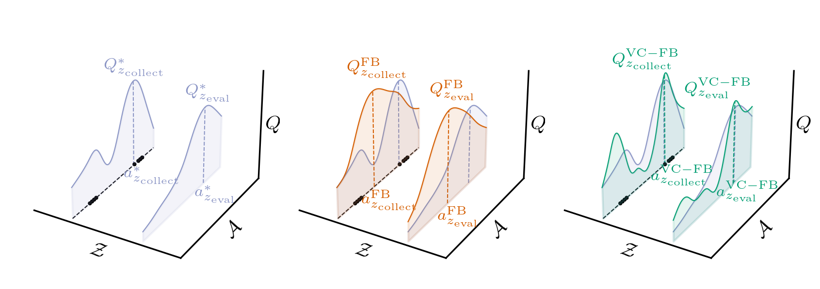
Figure 1: FB’s failure mode on sub-optimal datasets and VC-FB’s resolution.. (Left) Zero-shot RL methods must train on a dataset which was collected by a behaviour policy optimising against task $z_{\mathrm{collect}}$, yet generalise to new tasks $z_{\mathrm{eval}}$. Both tasks have associated optimal value functions $Q_{z_{\mathrm{collect}}}^{*}$ and $Q_{z_{\mathrm{eval}}}^{*}$ for a given marginal state. (Middle) Forward-backward (FB) representations overestimate the value of actions not in the dataset for all tasks. (Right) Value-conservative forward-backward (VC-FB) representations suppress the value of actions not in the dataset for all tasks. Black dots represent state-action samples present in the dataset.

2 Background

Preliminaries. We consider the standard RL setup of a Markov decision process (MDP) (Sutton & Barto, 2018). We focus on the class of continuous, finite-horizon MDPs, characterised by the tuple $(\mathcal{S},\mathcal{A},\mathcal{R},\mathcal{P},T,\gamma)$, where $\mathcal{S}\in\mathbb{R}^{n}$ and $\mathcal{A}\in\mathbb{R}^{m}$ are continuous spaces of environment states and agent actions, $\mathcal{P}:\mathcal{S}\times\mathcal{A}\mapsto\Delta(\mathcal{S})$ is a stochastic state transition function and $\mathcal{R}:\mathcal{S}\mapsto\mathbb{R}_{\geq 0}$ is a function mapping states to non-negative rewards (Bellman, 1957). At each timestep $t$, the agent observes state $s_{t}$, selects action $a_{t}$ according to a policy function $\pi(s_{t})$, transitions to the next state $s_{t+1}\sim\mathcal{P}(\cdot|s_{t},a_{t})$, and receives a reward $r_{t+1}=\mathcal{R}(s_{t+1})$. This process repeats until a terminal timestep $t=T$. The agent’s task is to learn a policy that maximises the expected discounted sum of rewards $\mathbb{E}_{\ \pi,\mathcal{P}}\sum_{t=0}^{T-1}\gamma^{t}\mathcal{R}(s_{t+1})$, where $\gamma\in[0,1]$ is a discount factor.

Problem formulation. We are interested in pre-training agents to solve any arbitrary task in an environment, where each task is characterised by a reward function $\mathcal{R}$. Therefore, instead of solving one MDP, we wish to solve a set of MDPs, each sharing the same structure bar the reward functions (Borsa et al., 2018). Touati et al. (2022) call this zero-shot RL, which is equivalent to multi-task offline RL with no downstream planning allowance (Lazaric, 2012; Levine et al., 2020). During the pre-training phase, we assume the agent has access to a static dataset of reward-free transitions $\mathcal{D}=\{(s_{i},a_{i},s_{i+1})\}_{i\in\{1,\ldots,k\}}$ generated by an unknown behaviour policy. Once a task is revealed downstream, the agent must return a good policy for that task with no further planning or learning.

Forward-backward representations. FB representations rely on successor measures, which generalise Dayan (1993)’s successor representations to continuous MDPs (Blier et al., 2021). A successor measure gives the expected discounted time spent in each subset of future states $S_{+}\subset\mathcal{S}$ after starting in state $s_{0}$, taking action $a_{0}$, and following policy $\pi$ thereafter:

$$M^{\pi}(s_{0},a_{0},S_{+}):=\textstyle{\sum_{t=0}^{T-1}}\gamma^{t}\Pr(s_{t+1}\in S_{+}|(s_{0},a_{0}),\pi),\;\forall\;S_{+}\subset\mathcal{S}.$$ (1)

For any reward function $\mathcal{R}$ and policy $\pi$, the state-action value ($Q$) function is the integral of $\mathcal{R}$ with respect to $M^{\pi}$:

$$Q^{\pi}_{\mathcal{R}}(s_{0},a_{0}):=\textstyle\int_{s_{+}\in\mathcal{S}}\mathcal{R}(s_{+})M^{\pi}(s_{0},a_{0},\text{d}s_{+}).$$ (2)

An FB representation approximates the successor measures of optimal policies for an infinite family of reward functions, and so can be thought of as a universal successor measure. It parameterises these policies $\pi_{z}$ by task vectors $z\in\mathbb{R}^{d}$. The representation consists of a forward model $F:\mathcal{S}\times\mathcal{A}\times\mathbb{R}^{d}\mapsto\mathbb{R}^{d}$, which outputs an embedding vector summarising the distribution of future states for a given state-action pair and policy, and a backward model $B:\mathcal{S}\mapsto\mathbb{R}^{d}$, which outputs an embedding vector summarising the distribution of states visited before a given state. Together, they form a rank-$d$ approximation to the successor measure for the entire policy family:

$$M^{\pi_{z}}(s_{0},a_{0},\text{d}s_{+})\approx F(s_{0},a_{0},z)^{\top}B(s_{+})\rho(\text{d}s_{+}),\;\forall\;s_{+}\in\mathcal{S},$$ (3)

where $\rho$ is the state marginal in the training dataset $\mathcal{D}$. Since the successor measure satisfies a Bellman equation, $F$ and $B$ can be trained to improve the approximation in Equation 3 across a distribution $\mathcal{Z}$ of task vectors via a temporal difference (TD) method (Samuel, 1959; Sutton, 1988):

$${}\mathcal{L}_{\text{FB}}=\mathbb{E}_{(s_{t},a_{t},s_{t+1},s_{+})\sim\mathcal{D},z\sim\mathcal{Z}}[\left(F(s_{t},a_{t},z)^{\top}B(s_{+})-\gamma\bar{F}(s_{t+1},\pi_{z}(s_{t+1}),z)^{\top}\bar{B}(s_{+})\right)^{2}\\ -2F(s_{t},a_{t},z)^{\top}B(s_{t+1})],$$ (4)

where $s_{+}$ is sampled independently from $(s_{t},a_{t},s_{t+1})$ and $\bar{F}$ and $\bar{B}$ are lagging target networks. See Touati et al. (2022) for a full derivation of this loss. By Equation 2, the trained representation can then be used to approximate the $Q$ function for any $\pi_{z}:z\sim\mathcal{Z}$ and reward function $\mathcal{R}$:

$$\begin{array}[]{ll}Q^{\pi_{z}}_{\mathcal{R}}(s_{0},a_{0})&\approx\textstyle\int_{s_{+}\in\mathcal{S}}\mathcal{R}(s_{+})F(s_{0},a_{0},z)^{\top}B(s_{+})\rho(\text{d}s_{+})\vspace{0.1cm}\\ &=F(s_{0},a_{0},z)^{\top}\mathbb{E}_{s_{+}\sim\rho}[\ \mathcal{R}(s_{+})B(s_{+})\ ].\end{array}$$ (5)

Touati et al. (2022) show that if the task vector $z$ and policy $\pi_{z}$ are defined as follows:

$$z=\mathbb{E}_{s_{+}\sim\rho}[\ \mathcal{R}(s_{+})B(s_{+})\ ];$$ (6)

$$\pi_{z}(s)=\text{argmax}_{a}F(s,a,z)^{\top}z;$$ (7)

and if $z$ lies within the task distribution $\mathcal{Z}$, we can expect $\pi_{z}$ to be a near-optimal policy for $\mathcal{R}$. The approximation becomes more exact as the embedding dimensionality $d$ grows. We thereby obtain a mechanism for zero-shot RL. In practice, given a dataset $\mathcal{D}_{\text{labelled}}$ of reward-labelled states distributed as $\rho$, we can approximate $z\approx\mathbb{E}_{(s,r)\sim\mathcal{D}_{\text{labelled}}}[\ rB(s)\ ]$ by simple averaging. For the special case of a goal-reaching task with goal $s_{g}$, the task vector can be defined directly as $z=B(s_{g})$. In theory, $\pi_{z}$ is then given analytically via Equation 7, but continuous action spaces necessitate learning a separate task-conditioned policy model in an actor-critic formulation (Lillicrap et al., 2016).

3 Conservative Forward-Backward Representations

We begin by examining the FB loss (Equation 4) more closely. The TD target includes an action produced by the current policy $a_{t+1}=\pi_{z}(s_{t+1})$. Equation 7 shows that this action is the current best estimate of the optimal action in state $s$ for task $z$. When training on a finite dataset, this maximisation does not constrain the policy to actions observed in the dataset, and so the policy can become biased towards out-of-distribution (OOD) actions thought to be of high value–a well-observed phenomenon in offline RL (Kumar et al., 2019; 2020). In such instances, the TD targets may be evaluated at state-action pairs outside the dataset, making them unreliable and causing errors in the measure and value predictions. Figure 2 shows the overestimation of $Q$ as dataset size and quality is varied. The smaller and less diverse the dataset, the more $Q$ values tend to be overestimated.

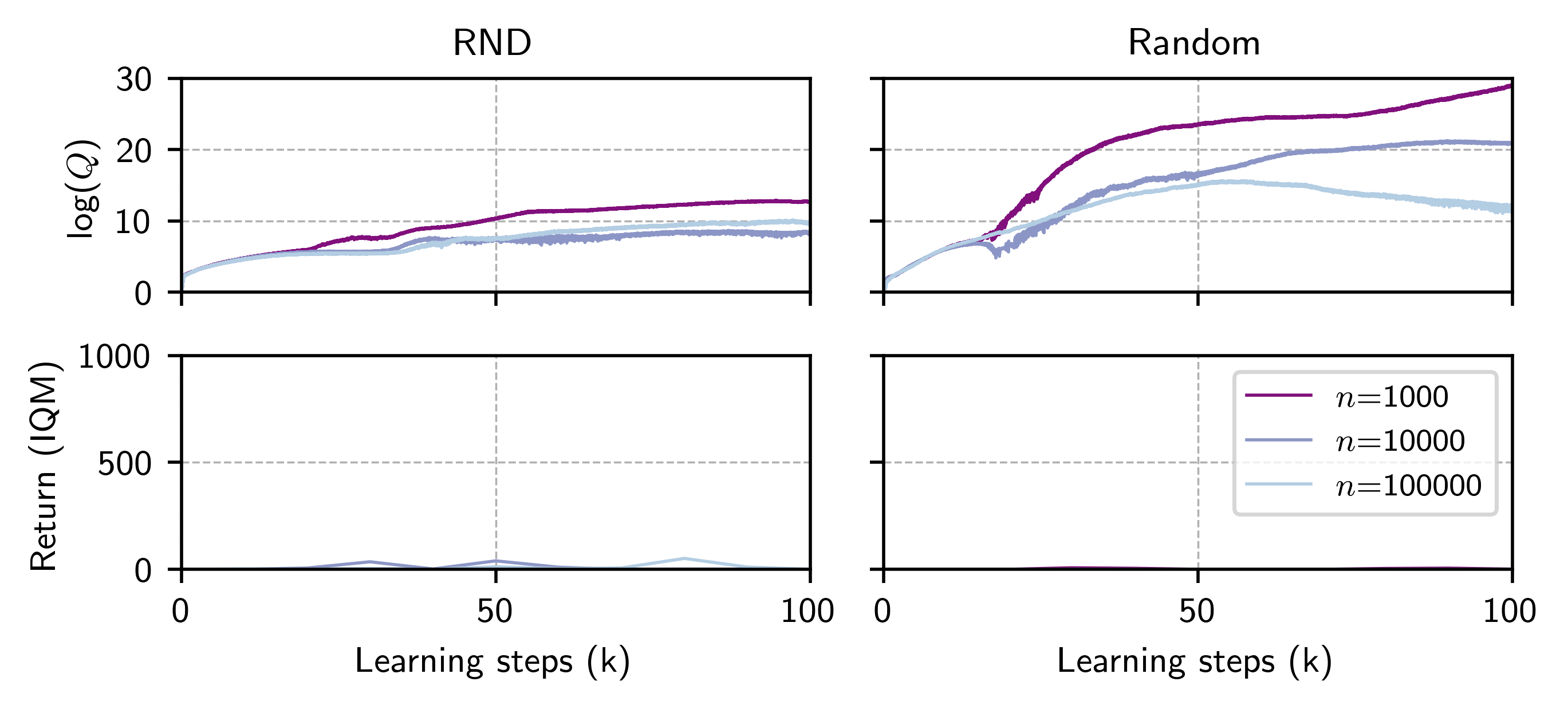
Figure 2: FB value overestimation with respect to dataset size $n$ and quality. Log $Q$ values and IQM of rollout performance on all Point-mass Maze tasks for datasets (a) Rnd and (b) Random. $Q$ values predicted during training increase as both the size and “quality” of the dataset decrease. This contradicts the low return of all resultant policies. Informally, we say the Rnd dataset is “high” quality, and the Random dataset is “low” quality–see Appendix A.2 for more details.

The canonical fix for value overestimation in offline RL is conservative $Q$-learning (CQL) (Kumar et al., 2019; 2020). Intuitively, CQL suppresses the values of OOD actions to be below those of in-distribution actions, and so approximately constrains the agent’s policy to actions observed in the dataset. To achieve this, a new term is added to the usual $Q$ loss function

$$\mathcal{L}_{\text{CQL}}={\color[rgb]{0.5078125,0.05859375,0.484375}{\alpha\cdot\left(\mathbb{E}_{s\sim\mathcal{D}}[\max_{a}Q(s,a)]-\mathbb{E}_{(s,a)\sim\mathcal{D}}[Q(s,a)]\right)}}+\mathcal{L}_{\text{Q}},$$ (8)

where $\alpha$ is a scaling parameter and $\mathcal{L}_{\text{Q}}$ represents the normal TD loss on $Q$. This proves to be a useful inductive bias, mitigating value overestimation and producing state-of-the-art results on many offline RL benchmark tasks (Fu et al., 2020).

We can replicate a similar inductive bias in the FB context, substituting $F(s,a,z)^{\top}z$ for $Q$ in Equation 8 and adding the normal FB loss (Equation 4)

$$\mathcal{L}_{\text{VC-FB}}={\color[rgb]{0.0078125,0.5625,0.40625}{\alpha\cdot\left(\mathbb{E}_{s\sim\mathcal{D},z\sim\mathcal{Z}}[\max_{a}F(s,a,z)^{\top}z]-\mathbb{E}_{(s,a)\sim\mathcal{D},z\sim\mathcal{Z}}[F(s,a,z)^{\top}z]\right)}}+\mathcal{L}_{\text{FB}}.$$ (9)

The key difference between Equations 8 and 9 is that the former suppresses the value of OOD actions for one task, whereas the latter does so for all tasks in an environment. We discuss the usefulness of this inductive bias in Section 3.1. We call models learnt with this loss value-conservative forward-backward representations (VC-FB).

Sampling uniformly from $\mathcal{Z}$ in Equation 9 may reduce values for tasks or goals that are never used in practice. Instead, it may prove better to direct updates towards tasks we are likely to encounter. To do so, we first recall that the backward embedding of a future state is equivalent to the task vector for reaching that state, i.e. $z_{+}=B(s_{+})$. Substituting this into Equation 9, we obtain a new loss that penalises OOD actions with respect to reaching some goal state $s_{+}$

$$\mathcal{L}_{\text{MC-FB}}={\color[rgb]{0.10546875,0.56640625,0.8203125}{\alpha\cdot\left(\mathbb{E}_{(s,s_{+})\sim\mathcal{D},z\sim\mathcal{Z}}[\max_{a}F(s,a,z)^{\top}B(s_{+})]-\mathbb{E}_{(s,a,s_{+})\sim\mathcal{D}}[F(s,a,z)^{\top}B(s_{+})]\right)}}\\ +\mathcal{L}_{\text{FB}}.$$ (10)

Whereas Equation 9 suppresses values of OOD actions for all tasks, Equation 10 suppresses the expected visitation count to goal state $s_{+}$ when taking an OOD action, because $M(s,a,z,s_{+})=F(s,a,z)^{\top}B(s_{+})$. As such, we call this variant a measure-conservative forward-backward representation (MC-FB). We note that this variant confines conservative penalties to the part of $z$-space occupied by the backward embeddings of $s_{+}\sim\mathcal{D}$, which in practice may be far smaller than the $z$-space coverage obtained via $z\sim\mathcal{Z}$. The effectiveness of each bias is explored in Section 4.

Practical implementations of conservative FB representations require two new model components: a conservative penalty scaling factor $\alpha$ and a way of computing the max operation over a continuous action space. Empirically, we observe fixed values of $\alpha$ leading to fragile performance, so dynamically tune it at each learning step using Lagrangian dual-gradient descent as per Kumar et al. (2020). Appendix B.1.4 discusses this procedure in more detail. The max operation is approximated by computing a log-sum exponential over a finite set of $Q$ values derived from a finite set of action samples. There are many ways to choose these samples, but again, we follow the recommendations of Kumar et al. (2020) and mix actions sampled uniformly from a random policy and the current policy. Appendix B.1.3 provides full detail. Code snippets demonstrating the required programmatic changes to vanilla FB implementation are provided in Appendix G. We emphasise these additions represent only a small increase in the number of lines required to implement FB.

3.1 A Didactic Example

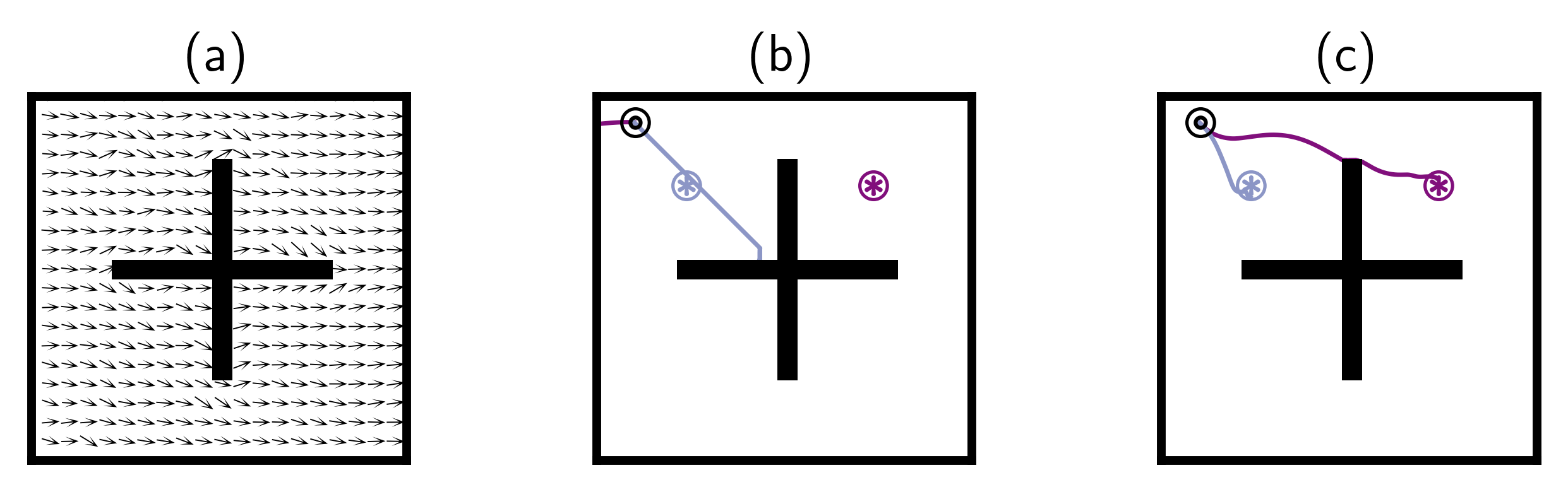
Figure 3: Ignoring out-of-distribution actions.. The agents are tasked with learning separate policies for reaching ${\color[rgb]{0.55078125,0.58984375,0.77734375}\circledast}$ and ${\color[rgb]{0.5078125,0.05859375,0.484375}\circledast}$. (a) Rnd dataset with all “left” actions removed; quivers represent the mean action direction in each state bin. (b) Best FB rollout after 1 million learning steps. (c) Best VC-FB performance after 1 million learning steps. FB overestimates the value of OOD actions and cannot complete either task; VC-FB synthesises the requisite information from the dataset and completes both tasks.

To understand situations in which a conservative world model may be useful, we introduce a modified version of Point-mass Maze from the ExORL benchmark (Yarats et al., 2022). Episodes begin with a point-mass initialised in the upper left of the maze ($\circledcirc$), and the agent is tasked with selecting $x$ and $y$ tilt directions such that the mass is moved towards one of two goal locations (${\color[rgb]{0.55078125,0.58984375,0.77734375}\circledast}$ and ${\color[rgb]{0.5078125,0.05859375,0.484375}\circledast}$). The action space is two-dimensional and bounded in $[-1,1]$. We take the Rnd dataset and remove all “left” actions such that $a_{x}\in[0,1]$ and $a_{y}\in[-1,1]$, creating a dataset that has the necessary information for solving the tasks, but is inexhaustive (Figure 3 (a)). We train FB and VC-FB on this dataset and plot the highest-reward trajectories–Figure 3 (b) and (c). FB overestimates the value of OOD actions and cannot complete either task. Conversely, VC-FB synthesises the requisite information from the dataset and completes both tasks.

The above example is engineered for exposition, but we expect conservatism to be helpful in more general contexts. Low-value actions for one task can often be low value for other tasks and, importantly, the more performant the behaviour policy, the less likely such low value actions are to be in the dataset. Consider the four tasks in the Walker environment: $\{\mathtt{walk},\mathtt{stand},\mathtt{run},\mathtt{flip}\}$, where all tasks require the robot to stand from a seated position before exemplifying different behaviours. If the dataset includes actions that are antithetical to standing, as might be the case if the behaviour policy used to collect the dataset is highly exploratory, then both FB and VC-FB can observe their low value across tasks. However, if the dataset does not include such actions, as might be the case if it was collected via a near-optimal controller that never fails to stand, then FB may overestimate the value of not standing across tasks, and VC-FB would correctly devalue them. We extend these observations to more varied environments in the section that follows.

4 Experiments

In this section we perform an empirical study to evaluate our proposals. We seek answers to three questions: (Q1) Can our proposals from Section 3 improve FB performance on small and/or low-quality datasets? (Q2) How does the performance of VC-FB and MC-FB vary with respect to task type and dataset diversity? (Q3) Do we sacrifice performance on full datasets for performance on small and/or low-quality datasets?

4.1 Setup

We respond to these questions using the ExORL benchmark, which provides datasets collected by unsupervised exploratory algorithms on the DeepMind Control Suite (Yarats et al., 2022; Tassa et al., 2018). We select three of the same domains as Touati & Ollivier (2021): Walker, Quadruped and Point-mass Maze, but substitute Jaco for Cheetah. This provides two locomotion domains and two goal-reaching domains. Within each domain, we evaluate on all tasks provided by the DeepMind Control Suite for a total of 17 tasks across four domains. Full details are provided in Appendix A.1.

We pre-train on three datasets of varying quality. Although there is no unambiguous metric for quantifying dataset quality, we use the reported performance of offline TD3 on Point-mass Maze for each dataset as a proxy. We choose datasets collected via Random Network Distillation (Rnd) (Burda et al., 2018), Diversity is All You Need (Diayn) (Eysenbach et al., 2018), and Random policies, where agents trained on Rnd are the most performant, on Diayn are median performers, and on Random are the least performant. As well as selecting for quality, we also select for size. The ExORL datasets have up to 10 million transitions per domain. We uniformly sub-sample 100,000 transitions from these to create datasets that may be considered more realistically sized for real-world applications. More details on the datasets are provided in Appendix A.2, which includes a visualisation of the state coverage for each dataset on Point-mass Maze (Figure 6).

4.2 Baselines

We use FB as described in Touati et al. (2022) as our sole zero-shot RL baseline. Though other methods exist, we believe the performance gap they report is sufficient that we can rule out any other methods as state-of-the-art. As single-task RL baselines, we use CQL and offline TD3 trained on the same datasets relabelled with task rewards. CQL is representative of what a conservative algorithm can achieve when optimising for one task in a domain rather than all tasks. Offline TD3 exhibits the best aggregate single-task performance on the ExORL benchmark, so it should be indicative of the maximum performance we could expect to extract from a dataset. Full implementation details and hyperparameters are provided in Appendix B.2 and B.3.

We evaluate the performance of VC-FB, MC-FB and our baselines across five random seeds. To mitigate the well-established pitfalls of stochastic RL algorithm evaluation, we employ the best practice recommendations of Agarwal et al. (2021) when reporting observed performance. Concretely, we run each algorithm for 1 million learning steps, evaluating performance at checkpoints of 20,000 steps. At each checkpoint, we perform 10 rollouts and record the interquartile mean performance across each task. We then calculate the interquartile mean of performance across seeds for each checkpoint to create the learning curves reported in Appendix F. Results are reported with 95% confidence intervals obtained via stratified bootstrapping (Efron, 1992). Full implementation details are provided in Appendix B.1.

4.3 Results

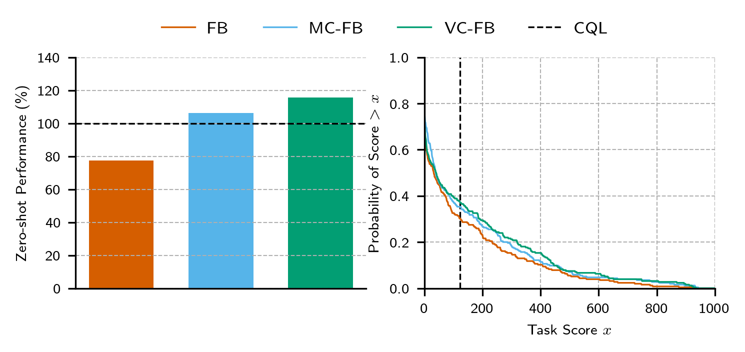
Figure 4: Aggregate zero-shot performance. (Left): IQM of task scores across datasets and domains, normalised against the performance of CQL, our baseline. (Right) Performance profiles showing the distribution of scores across all tasks and domains. Both conservative FB variants stochastically dominate vanilla FB. The black dashed line represents the IQM of CQL performance across all datasets, domains, tasks and seeds.

Q1. We report the aggregate performance of all FB algorithms and CQL in Figure 4. Both MC-FB and VC-FB stochastically dominate FB, achieving 150% and 137% its performance respectively. MC-FB and VC-FB outperform our single-task baseline in expectation, reaching 111% and 120% of CQL performance respectively despite not having access to task-specific reward labels and needing to fit policies for all tasks. This is a surprising result, and to the best of our knowledge, the first time a multi-task offline agent has been shown to outperform a single-task analogue. CQL outperforms offline TD3 in aggregate, so we drop offline TD3 from the core analysis, but report its full results in Appendix C alongside all other methods. We note FB achieves 80% of single-task offline TD3, which roughly aligns with the 85% performance on the full datasets reported by Touati et al. (2022).

Q2. We decompose the methods’ performance with respect to domain and dataset diversity in Figure 5. The largest gap in performance between the conservative FB variants and FB is on Rnd, the highest-quality dataset. VC-FB and MC-FB reach 253% and 184% of FB performance respectively, and outperform CQL on three of the four domains. On Diayn, the conservative variants outperform all methods and reach 135% of CQL’s score. On the Random dataset, all methods perform similarly poorly, except for CQL on Jaco, which significantly outperforms all methods. However, in general, these results suggest the Random dataset is not informative enough to extract valuable policies. There appears to be little correlation between the type of domain (Appendix A.1) and the score achieved by any method.

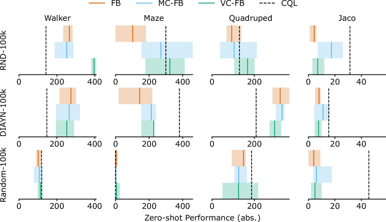
Figure 5: Performance by dataset and domain. IQM scores across tasks and seeds with 95% confidence intervals. In general, the conservative FB variants perform better as dataset quality improves.

Q3. We report the performance of all FB methods across all domains when trained on the full Rnd dataset in Table 1. Both conservative FB variants maintain (and slightly exceed) the performance of vanilla FB in expectation and exhibit identical aggregate performance. These results suggest that performance on large, diverse datasets does not suffer as a consequence of the design decisions made to improve performance on our small datasets that lack diversity. Therefore, we can safely adopt conservatism into FB without worrying about performance trade-offs.

Table 1: Performance on full Rnd dataset. Aggregated IQM scores for all tasks with 95% confidence intervals, averaged across three seeds. Both VC-FB and MC-FB maintain the performance of FB.

Domain	Task	FB	VC-FB	MC-FB
Walker	all tasks	639 (616–661)	659 (647–670)	651 (632–671)
Quadruped	all tasks	656 (638–674)	579 (522–635)	635 (628–642)
Maze	all tasks	219 (86–353)	287 (117–457)	261 (159–363)
Jaco	all tasks	39 (29–50)	33 (24–42)	34 (18–51)
All	all tasks	361	381	381

5 Discussion and Limitations

Performance discrepancy between conservative variants. VC-FB outperforms MC-FB in aggregate, but not in every constituent domain, which raises the question of when one variant should be selected over the other. Suppose the tasks in our domain of interest are distributed uniformly in $z$-space. In that case, we should expect VC-FB to outperform MC-FB as its conservative updates will match the underlying task distribution. Equally, if the tasks are clustered around state embeddings in $z$-space, then we should expect MC-FB to outperform VC-FB. In our experiments, we assumed the locomotion tasks would be distributed near-uniformly in $z$-space, and the goal-reaching tasks would be clustered around the goal state embeddings, thus implying better VC-FB performance on locomotion tasks and better MC-FB performance on goal-reaching tasks. There is little evidence to support this hypothesis. It seems intuiting the distribution of tasks in $z$-space a priori, and thus selecting the correct model, is non-trivial and requires careful further investigation. If progress can be made here, then $\mathcal{Z}$ could be tuned to better match the underlying task distribution of the domain, conservative updates could be made with respect to this improved $\mathcal{Z}$, and performance of all methods may improve.

Computational expense of conservative variants. The max value estimator used by the conservative FB variants performs log-sum-exponentials and concatenations across large tensors, both of which are expensive operations. We find that these operations, which are the primary contributors to the additional run-time, increase the training duration by approximately 3$\times$ over vanilla FB. An FB training run takes approximately 4 hours on an A100 GPU, whereas the conservative FB variants take approximately 12 hours. It seems highly likely that more elegant implementations exist that would improve training efficiency. We leave such an exploration for future work.

Learning instability. We report the learning curves for all algorithms across domains, datasets, and tasks in Appendix F. We note many instances of instability which would require practitioners to invoke early stopping. However, both CQL and offline TD3, our task-specific baselines, exhibit similar instability, so we do not consider this behaviour to be an inherent flaw of any method, but rather an indication of the difficulty of learning representations from sub-optimal data. Future work that stabilises FB learning dynamics could boost performance and simplify their deployment by negating the need for early stopping.

We provide detail of negative results in Appendix D to help inform future research.

6 Related Work

Conservatism in offline RL. The need for conservatism in offline RL was first highlighted by Fujimoto et al. (2019) in which they propose batch-constrained $Q$-learning (BCQ), a method for aligning the distributions of agent and behaviour policies, as a remedy. Instead of operating on policies, Kumar et al. (2020)’s CQL operates on values, suppressing the value of OOD actions to be lower than in-distribution actions. More recently, Lyu et al. (2022) provided an improved lower bound on the performance of CQL with mildly conservative $Q$-learning (MCQ) which is less conservative on OOD actions close to the dataset that are often higher value than vanilla CQL predicts. They prove that MCQ induces policies that are at least as performant as the behaviour policy. We note that these methods could be directly ported into our proposal, which may improve performance further.

The most similar works to ours are Kidambi et al. (2020) and Yu et al. (2020); both are model-based offline RL methods that employ conservatism in the context of a dynamics model. Kidambi et al. (2020) suppress the reward of predicted rollouts using a binary operator that determines whether the rollout is within dataset support, and Yu et al. (2020) suppress rewards in proportion to the uncertainty of rollouts as predicted by their dynamics model. Both are analogous to our OOD value suppression in VC-FB, but are limited to the single-task setting and require a planning algorithm to optimise the policy at test time. To our knowledge, the only work that studies zero-shot RL with sub-optimal data is Kumar et al. (2022)’s work on scaling CQL. In multi-task Atari, they train one base network on a large, diverse dataset of sub-optimal trajectories, then optimise separate actor heads for each Atari task. They show that, provided a sufficiently large dataset, high parameter count CQL networks can outperform the behaviour policy that created the dataset. However, the generality of this approach is limited by the need for a separate head per task, meaning we need to enumerate the tasks we wish to solve a priori. The parameterisation by task vectors $z$ means that FB (and hence, our approach) automatically learns policies for all tasks without such enumeration.

World models. The canonical multi-task model is Schaul et al. (2015)’s universal value function approximator (UVFA), which conditions state-action value predictions on tasks and can be used by a planning algorithm to return a task-conditioned policy. The planning requirement is removed by Barreto et al. (2017)’s successor features, enabling policies to be returned from UVFA-style models using only rudimentary matrix operations. These works laid the foundations for universal successor features (Borsa et al., 2018) and FB representations (Touati & Ollivier, 2021; Touati et al., 2022) that can return policies for any task in an environment instantly after a pre-training phase. Sekar et al. (2020)’s Plan2Explore showed agents can synthesise policies zero-shot that are comparable with those obtained via single-task when trained solely inside a world model. Ghosh et al. (2023)’s intention-conditioned value functions can be thought of as FB representations without actions, and so predict how states evolve with respect to a task, i.e. $(s,z)\leadsto s_{+}$ rather than $(s,a,z)\leadsto s_{+}$. This is helpful as it allows representations to be learnt from data without action or reward labels, increasing the scope of datasets on which RL algorithms can be trained. To our knowledge, no prior work has acknowledged the deficiencies of any of these models with sub-optimal datasets, and no work has attempted to augment these models with conservatism.

7 Conclusion

In this paper, we explored training agents to perform zero-shot reinforcement learning (RL) with sub-optimal data. We established that the existing state-of-the-art method, FB representations, suffer in this regime because they overestimate the value of out-of-distribution state-action values. As a resolution, we proposed a family of conservative FB algorithms that suppress either the values (VC-FB) or measures (MC-FB) of out-of-distribution state-action pairs. In experiments across various domains, tasks and datasets, we showed our proposals outperform vanilla FB by up to 150% in aggregate and surpass our task-specific baseline despite lacking access to reward labels a priori. In addition to improving performance when trained on sub-optimal datasets, we showed that performance on large, diverse datasets does not suffer as a consequence of our design decisions. Our proposals are a step towards the use of zero-shot RL methods in the real world.

Acknowledgments

We thank Sergey Levine for helpful feedback on the core and finetuning experiments, and Alessandro Abate and Yann Ollivier for reviewing earlier versions of this manuscript. Computational resources were provided by the Cambridge Centre for Data-Driven Discovery (C2D3) and Bristol Advanced Computing Research Centre (ACRC). This work was supported by an EPSRC DTP Studentship (EP/T517847/1) and Emerson Electric.

Appendices

Appendix A Experimental Details

A.1 Domains

We consider two locomotion and two goal-directed domains from the ExORL benchmark (Yarats et al., 2022) which is built atop the DeepMind Control Suite (Tassa et al., 2018). Environments are visualised here: https://www.youtube.com/watch?v=rAai4QzcYbs. The domains are summarised in Table 2.

Walker. A two-legged robot required to perform locomotion starting from bent-kneed position. The state and action spaces are 24 and 6-dimensional respectively, consisting of joint torques, velocities and positions. ExORL provides four tasks stand, walk, run and flip. The reward function for stand motivates straightened legs and an upright torse; walk and run are supersets of stand including reward for small and large degrees of forward velocity; and flip motivates angular velocity of the torso after standing. Rewards are dense.

Quadruped. A four-legged robot required to perform locomotion inside a 3D maze. The state and action spaces are 78 and 12-dimensional respectively, consisting of joint torques, velocities and positions. ExORL provides five tasks stand, roll, roll fast, jump and escape. The reward function for stand motivates a minimum torse height and straightened legs; roll and roll fast require the robot to flip from a position on its back with varying speed; jump adds a term motivating vertical displacement to stand; and escape requires the agent to escape from a 3D maze. Rewards are dense.

Point-mass Maze. A 2D maze with four rooms where the task is to move a point-mass to one of the rooms. The state and action spaces are 4 and 2-dimensional respectively; the state space consists of $x,y$ positions and velocities of the mass, the action space is the $x,y$ tilt angle. ExORL provides four reaching tasks top left, top right, bottom left and bottom right. The mass is always initialised in the top left and the reward is proportional to the distance from the goal, though is sparse i.e. it only registers once the agent is reasonably close to the goal.

Jaco. A 3D robotic arm tasked with reaching an object. The state and action spaces are 55 and 6-dimensional respectively and consist of joint torques, velocities and positions. ExORL provides four reaching tasks top left, top right, bottom left and bottom right. The reward is proportional to the distance from the goal object, though is sparse i.e. it only registers once the agent is reasonably close to the goal object.

Table 2: Experimental domain summary. Dimensionality refers to the relative size of state and actions spaces. Type is the task categorisation, either locomotion (satisfy a prescribed behaviour until the episode ends) or goal-reaching (achieve a specific task to terminate the episode). Reward is the frequency with which non-zero rewards are provided, where dense refers to non-zero rewards at every timestep and sparse refers to non-zero rewards only at positions close to the goal. Green and red colours reflect the relative difficulty of these settings.

Domain	Dimensionality	Type	Reward
Walker	Low	Locomotion	Dense
Quadruped	High	Locomotion	Dense
Point-mass Maze	Low	Goal-reaching	Sparse
Jaco	High	Goal-reaching	Sparse

A.2 Datasets

We train on 100,000 transitions uniformly sampled from three datasets on the ExORL benchmark collected by different unsupervised agents: Random, Diayn, and Rnd. The state coverage on Point-mass maze is depicted in Figure 6. Though harder to visualise, we found that state marginals on higher-dimensional tasks (e.g. Walker) showed a similar diversity in state coverage.

Rnd. An agent whose exploration is directed by the predicted error in its ensemble of dynamics models. Informally, we say Rnd datasets exhibit high state diversity.

Diayn. An agent that attempts to sequentially learn a set of skills. Informally, we say Diayn datasets exhibit medium state diversity.

Random. A agent that selects actions uniformly at random from the action space. Informally, we say Random datasets exhibit low state diversity.

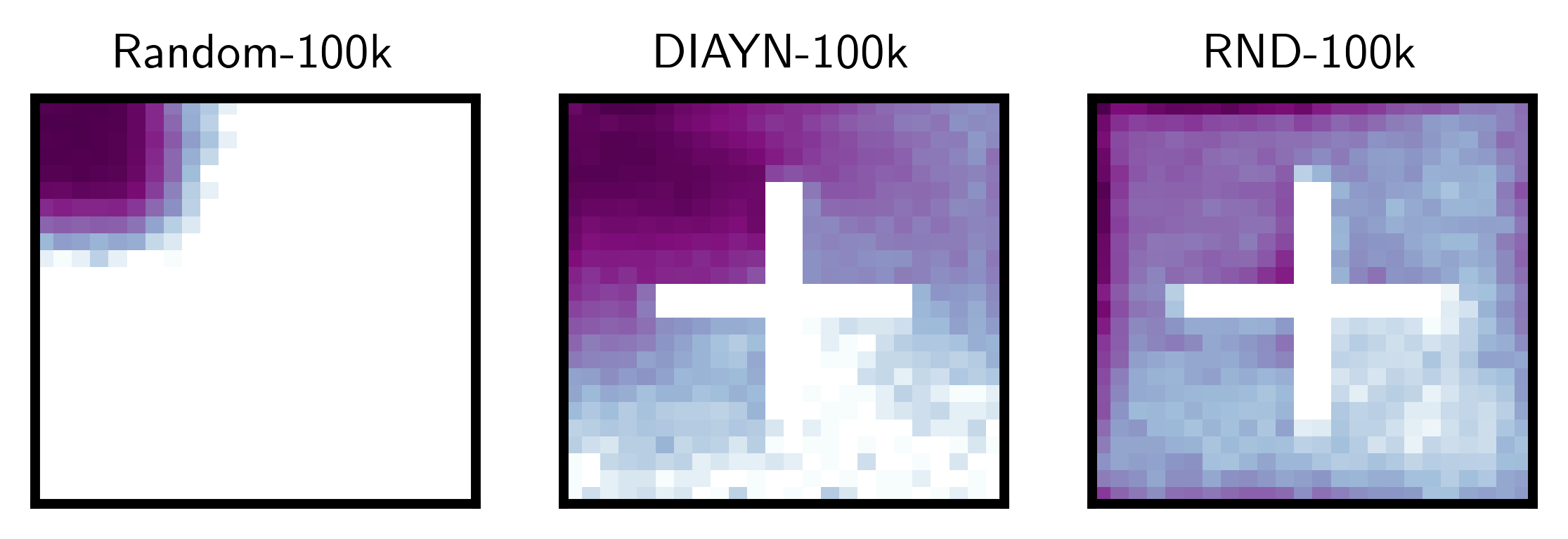
Figure 6: Point-mass maze state coverage by dataset. (left) Random; (middle) Diayn; (right) Rnd.

Appendix B Implementations

Here we detail implementations for all methods discussed in this paper. The code required to reproduce our experiments is provided open-source at: https://github.com/enjeeneer/conservative-world-models.

B.1 Forward-Backward Representations

B.1.1 Architecture

The forward-backward architecture described below follows the original implementation by Touati et al. (2022) exactly, other than the batch size which we reduce from 1024 to 512. We did this to reduce the computational expense of each run without limiting performance. The hyperparameter study in Appendix J of Touati et al. (2022) shows this choice is unlikely to affect FB performance. We summarise their implementation here for the reader’s benefit. Hyperparameters are reported in Table 3.

Forward Representation $F(s,a,z)$. The input to the forward representation $F$ is always preprocessed. State-action pairs $(s,a)$ and state-task pairs $(s,z)$ have their own preprocessors $P_{F}^{1}$ and $P_{F}^{2}$. $P_{F}^{1}$ and $P_{F}^{2}$ are feedforward MLPs that embed their inputs into a 512-dimensional space. These embeddings are concatenated and passed through a third feedforward MLP $F$ which outputs a $d$-dimensional vector, where $d$ is our final latent dimension.

Backward Representation $B(s)$. The backward representation $B$ is a feedforward MLP that takes a state as input and outputs an $L2$-normalised, $d$-dimensional latent embedding.

Actor $\pi(s,z)$. Like the forward representation, the inputs to the policy network are similarly preprocessed. State-action pairs $(s,a)$ and state-task pairs $(s,z)$ have their own preprocessors $P_{\pi}^{1}$ and $P_{\pi}^{2}$. $P_{\pi}^{1}$ and $P_{\pi}^{2}$ are feedforward MLPs that embed their inputs into a 512-dimensional space. These embeddings are concatenated and passed through a third feedforward MLP which outputs a $a$-dimensional vector, where $a$ is the action-space dimensionality. A Tanh activation is used on the last layer to normalise their scale. As per Fujimoto et al. (2019)’s recommendations, the policy is smoothed by adding Gaussian noise $\sigma$ to the actions during training.

Misc. Layer normalisation (Ba et al., 2016) and Tanh activations are used in the first layer of all MLPs to standardise the inputs.

Table 3: (VC/MC)-FB Hyperparameters. The additional hyperparameters for Conservative FB representations are highlighted in blue.

Hyperparameter	Value
Latent dimension $d$	50 (100 for maze)
$F$ hidden layers	2
$F$ hidden dimension	1024
$B$ hidden layers	3
$B$ hidden dimension	256
$P_{F}$ hidden layers	2
$P_{F}$ hidden dimension	1024
$P_{\pi}$ hidden layers	2
$P_{\pi}$ hidden dimension	1024
Std. deviation for policy smoothing $\sigma$	0.2
Truncation level for policy smoothing	0.3
Learning steps	1,000,000
Batch size	512
Optimiser	Adam
Learning rate	0.0001
Discount $\gamma$	0.98 (0.99 for maze)
Activations (unless otherwise stated)	ReLU
Target network Polyak smoothing coefficient	0.01
$z$-inference labels	100,000
$z$ mixing ratio	0.5
Conservative budget $\tau$	50
OOD action samples per policy $N$	3

B.1.2 $z$ Sampling

FB representations require a method for sampling the task vector $z$ at each learning step. Touati et al. (2022) employ a mix of two methods, which we replicate:

1. Uniform sampling of $z$ in the hypersphere of radius $\sqrt{d}\in\mathbb{R}^{d}$,

2. Biased sampling of $z$ by passing states $s\sim\mathcal{D}$ through the backward representation $z=B(s)$.

We sample $z$ 50:50 from these methods at each learning step.

B.1.3 Maximum Value Approximator

The conservative variants of FB require a method of estimating $\max_{a}Q(s,a)$ which is intractable for continuous MDP. We follow Kumar et al. (2020)’s approach for convenience, though other options are available. We sample across the action-space and compute the log-sum-exponential of their associated $Q$ values to estimate the maximum $Q$ value. Kumar et al. (2020) combine actions sampled uniformly at random, actions from the current policy at the current timestep, and actions from the current policy at the following timestep. For VC-FB, the log-sum-exponential is computed as follows

$$\begin{aligned} \log\sum_{a}\exp F(s_{t},a_{t},z)^{\top}z&=\log(\frac{1}{3}\sum_{a}\exp(F(s_{t},a_{t},z)^{\top}z)+\frac{1}{3}\sum_{a}\exp(F(s_{t},a_{t},z)^{\top}z)\\ &\qquad+\frac{1}{3}\sum_{a}\exp(\exp(F(s_{t},a_{t},z)^{\top}z))),\\ &=\log(\frac{1}{3}\mathbb{E}_{a_{t}\sim\text{Unif}(\mathcal{A})}\left[\frac{\exp(F(s_{t},a_{t},z)^{\top}z)}{\text{Unif}(\mathcal{A})}\right]+\frac{1}{3}\mathbb{E}_{a_{t}\sim\pi(a_{t}|s_{t})}\left[\frac{\exp(F(s_{t},a_{t},z^{\top}z)}{\pi(a_{t}|s_{t})}\right]\\ &\qquad\frac{1}{3}\mathbb{E}_{a_{t+1}\sim\pi(a_{t+1}|s_{t+1})}\left[\frac{\exp(F(s_{t},a_{t+1},z)^{\top}z)}{\pi(a_{t+1}|s_{t+1})}\right]),\\ &=\log(\frac{1}{3N}\sum_{a_{i}\sim\text{Unif}(\mathcal{A})}^{N}\left[\frac{\exp(F(s_{t},a_{i},z)^{\top}z)}{\text{Unif}(\mathcal{A})}\right]+\frac{1}{6N}\sum_{a_{i}\sim\pi(a_{t}|s_{t})}^{2N}\left[\frac{\exp(F(s_{t},a_{i},z^{\top}z)}{\pi(a_{i}|s_{t})}\right]\\ &\qquad\frac{1}{3N}\sum_{a_{i}\sim\pi(a_{t+1}|s_{t+1})}^{N}\left[\frac{\exp(F(s_{t},a_{i},z)^{\top}z)}{\pi(a_{i}|s_{t+1})}\right]),\\ \end{aligned}$$ (11)

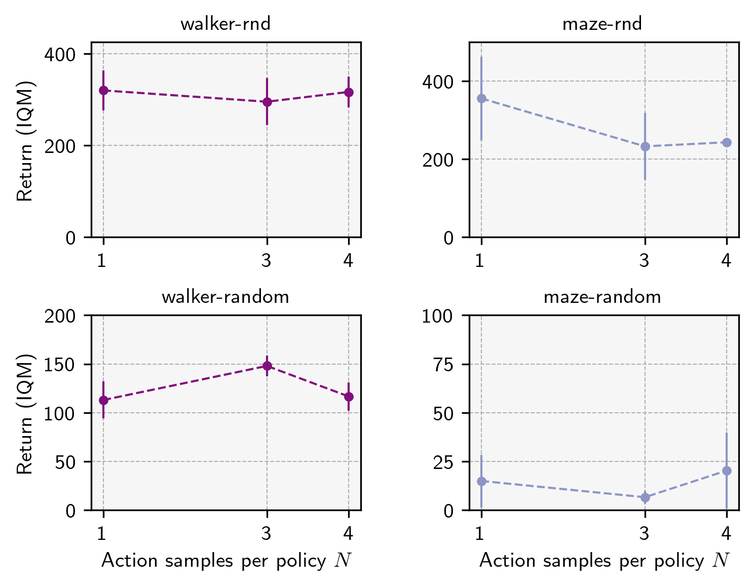
Figure 11: MC-FB sensitivity to action samples per policy $N$ on Walker and Point-mass Maze. Top: RND dataset; bottom: Random dataset. Maximum IQM return across the training run averaged over 3 random seeds.

with $N$ a hyperparameter defining the number of actions to sample across the action-space. Note: we sample twice as many actions from the current timestep/policy than from the uniform policy, or from the next timestep. In Appendix E, Figure 11 we show how the performance of VC-FB varies with the number of action samples. In general, performance improves with the number of action samples, but we limit $N=3$ to limit computational burden. The formulation for MC-FB is identical other than each value $F(s,a,z)^{T}z$ being replaced with measures $F(s,a,z)^{T}B(s_{+})$.

B.1.4 Dynamically Tuning $\alpha$

A critical hyperparameter is $\alpha$ which weights the conservative penalty with respect to other losses during each update. We initially trialled constant values of $\alpha$, but found performance to be fragile to this selection, and lacking robustness across environments. Instead, we follow Kumar et al. (2020) once again, and instantiate their algorithm for dynamically tuning $\alpha$, which they call Lagrangian dual gradient-descent on $\alpha$. We introduce a conservative budget parameterised by $\tau$, and set $\alpha$ with respect to this budget:

$$\min_{FB}{\color[rgb]{0.5078125,0.05859375,0.484375}{\max_{\alpha\geq 0}}\;\alpha}\cdot\left(\mathbb{E}_{s\sim\mathcal{D},z\sim\mathcal{Z}}[\max_{a}F(s,a,z)^{\top}z]-\mathbb{E}_{(s,a)\sim\mathcal{D},z\sim\mathcal{Z}}[F(s,a,z)^{\top}z]-{\color[rgb]{0.5078125,0.05859375,0.484375}{\tau}}\right)+\mathcal{L}(F,B).$$ (12)

Intuitively, this implies that if the scale of overestimation $\leq\tau$ then $\alpha$ is set close to 0, and the conservative penalty does not affect the updates. If the scale of overestimation $\geq\tau$ then $\alpha$ is set proportionally to this gap, and thus the conservative penalty is proportional to the degree of overestimation above $\tau$. As above, for the MC-FB variant values $F(s,a,z)^{\top}z$ are replaced with measures $F(s,a,z)^{\top}B(s_{+})$.

B.1.5 Algorithm

We summarise the end-to-end implementation of VC-FB as pseudo-code in Algorithm 1. MC-FB representations are trained identically other than at line 10 where the conservative penalty is computed for $M$ instead of $Q$, and in line 12 where $M$s are lower bounded via Equation 10.

Algorithm 1 Pre-training value-conservative forward-backward representations

0:  $\mathcal{D}$: dataset of trajectories           $F_{\theta_{F}}$, $B_{\theta_{B}}$, $\pi$: randomly initialised networks          $N$, $\mathcal{Z}$, $\nu$, $b$: learning steps, z-sampling distribution, polyak momentum, batch size

1:  for learning step $n=1...N$ do

2:     $\{(s_{i},a_{i},s_{i+1})\}\sim\mathcal{D}_{i\in|b|}$                                                     $\vartriangleleft$ Sample mini-batch of transitions

3:     $\{z_{i}\}_{i\in|b|}\sim\mathcal{Z}$                                                                                $\vartriangleleft$ Sample zs (Appendix B.1.2)

4:     

5:     // FB Update

6:     $\{a_{i+1}\}\sim\pi(s_{i+1},z_{i})$                              $\vartriangleleft$ Sample batch of actions at next states from policy

7:     Update $FB$ given $\{(s_{i},a_{i},s_{i+1},a_{i+1},z_{i})\}$                                                          $\vartriangleleft$ Equation 4

8:     

9:     // Conservative Update

10:     $Q^{\text{max}}(s_{i},a_{i})\approx\log\sum_{a}\exp F(s_{i},a_{i},z_{i})^{T}z_{i}$  $\vartriangleleft$ Compute conservative penalty (Equation 11)

11:     Compute $\alpha$ given $Q^{\text{max}}$ via Lagrangian dual gradient-descent                           $\vartriangleleft$ Equation 12

12:     Lower bound $Q$                                                                                                   $\vartriangleleft$ Equation 9

13:     

14:     // Actor Update

15:     $\{a_{i}\}\sim\pi(s_{i},z_{i})$                                                                           $\vartriangleleft$ Sample actions from policy

16:     Update actor to maximise $\mathbb{E}[F(s_{i},a_{i},z_{i})^{\top}z_{i}$]                     $\vartriangleleft$ Standard actor-critic formulation

17:     

18:     // Update target networks via polyak averaging

19:     $\theta_{F}^{-}\leftarrow\nu\theta_{F}^{-}+(1-\nu)\theta_{F}$                                                                  $\vartriangleleft$ Forward target network

20:     $\theta_{B}^{-}\leftarrow\nu\theta_{B}^{-}+(1-\nu)\theta_{B}$                                                               $\vartriangleleft$ Backward target network

21:  end for

B.2 CQL

B.2.1 Architecture

We adopt the same implementation and hyperparameters as is used on the ExORL benchmark. CQL inherits all functionality from a base soft actor-critic agent (Haarnoja et al., 2018), but adds a conservative penalty to the critic updates (Equation 8). Hyperparameters are reported in Table 4.

Critic(s). CQL employs double Q networks, where the target network is updated with Polyak averaging via a momentum coefficient. The critics are feedforward MLPs that take a state-action pair $(s,a)$ as input and output a value $\in\mathbb{R}^{1}$.

Actor. The actor is a standard feedforward MLP taking the state $s$ as input and outputting an $2a$-dimensional vector, where $a$ is the action-space dimensionality. The actor predicts the mean and standard deviation of a Gaussian distribution for each action dimension; during training a value is sampled at random, during evaluation the mean is used.

B.3 TD3

B.3.1 Architecture

We adopt the same implementation and hyperparameters as is used on the ExORL benchmark. Hyperparameters are reported in Table 4.

Critic(s). TD3 employs double Q networks, where the target network is updated with Polyak averaging via a momentum coefficient. The critics are feedforward MLPs that take a state-action pair $(s,a)$ as input and output a value $\in\mathbb{R}^{1}$.

Actor. The actor is a standard feedforward MLP taking the state $s$ as input and outputting an $a$-dimensional vector, where $a$ is the action-space dimensionality. The policy is smoothed by adding Gaussian noise $\sigma$ to the actions during training.

Misc. As is usual with TD3, layer normalisation (Ba et al., 2016) is applied to the inputs of all networks.

Table 4: Offline RL baseline algorithms hyperparameters.

Hyperparameter	CQL	TD3
Critic hidden layers	2	2
Critic hidden dimension	1024	1024
Actor hidden layers	2	2
Actor hidden dimension	1024	1024
Learning steps	1,000,000	1,000,000
Batch size	1024	1024
Optimiser	Adam	Adam
Learning rate	0.0001	0.0001
Discount $\gamma$	0.98 (0.99 for maze)	0.98 (0.99 for maze)
Activations	ReLU	ReLU
Target network Polyak smoothing coefficient	0.01	0.01
Sampled Actions Number	3	-
$\alpha$	0.01	-
Lagrange	False	-
Std. deviation for policy smoothing $\sigma$	-	0.2
Truncation level for policy smoothing	-	0.3

Appendix C Full Results

Table 5: Full experimental results. For each dataset-domain pair, we report the score at the step for which the all-task IQM is maximised when averaging across 5 seeds, and the constituent task scores at that step. Bracketed numbers represent the 95% confidence interval obtained by a stratified bootstrap.

			TD3	CQL	FB	VC-FB	MC-FB
Dataset	Domain	Task
Rnd-100k	walker	walk	210 (205–231)	138 (128–140)	184 (108–274)	446 (435–460)	247 (137–318)
		stand	362 (335–379)	386 (374–391)	558 (500–637)	624 (603–639)	480 (401–517)
		run	84 (78–90)	71 (63–75)	101 (88–144)	179 (159–194)	106 (72–145)
		flip	162 (148–171)	153 (130–172)	163 (90–203)	325 (294–350)	164 (120–198)
		all tasks	189 (177–200)	142 (135–149)	266 (233–283)	396 (381–407)	252 (188–288)
	quadruped	stand	119 (9–342)	167 (73–266)	134 (91–188)	331 (199–405)	171 (71–369)
		roll fast	63 (4–180)	93 (18–219)	83 (57–127)	141 (87–191)	81 (21–194)
		roll	96 (8–272)	251 (126–330)	139 (68–234)	141 (98–212)	132 (40–251)
		jump	85 (7–255)	128 (65–223)	121 (79–193)	159 (105–212)	97 (37–191)
		escape	3 (0–10)	3 (2–4)	7 (3–12)	8 (3–15)	5 (1–12)
		all tasks	81 (6–230)	129 (70–207)	93 (69–137)	168 (104–201)	104 (38–212)
	point-mass maze	reach top right	457 (0–733)	433 (275–558)	0 (0–26)	0 (0–203)	99 (9–377)
		reach top left	921 (895–938)	561 (493–717)	384 (0–724)	662 (218–903)	723 (363–895)
		reach bottom right	0 (0–0)	0 (0–0)	0 (0–0)	0 (0–0)	0 (0–0)
		reach bottom left	85 (22–295)	253 (102–451)	0 (0–0)	479 (70–748)	384 (0–776)
		all tasks	345 (171–405)	299 (262–364)	102 (0–181)	323 (177–412)	270 (154–459)
	jaco	reach top right	0 (0–0)	37 (21–53)	0 (0–3)	1 (0–4)	17 (8–29)
		reach top left	0 (0–0)	21 (12–35)	2 (1–4)	2 (0–3)	9 (1–21)
		reach bottom right	0 (0–0)	37 (21–53)	0 (0–6)	5 (2–21)	16 (6–25)
		reach bottom left	0 (0–0)	20 (17–28)	7 (3–15)	4 (1–21)	11 (1–45)
		all tasks	0 (0–0)	31 (25–36)	4 (1–6)	7 (3–12)	17 (7–26)
	all domains	all tasks	135	136	97	245	178
Diayn-100k	walker	walk	150 (132–167)	147 (118–201)	251 (158–315)	262 (141–370)	261 (175–351)
		stand	263 (235–306)	406 (365–455)	498 (381–652)	455 (401–492)	423 (375–595)
		run	46 (44–48)	38 (33–43)	98 (79–114)	83 (75–94)	81 (71–108)
		flip	163 (152–174)	149 (116–182)	193 (136–212)	229 (195–249)	183 (150–239)
		all tasks	154 (142–176)	147 (134–172)	274 (214–301)	252 (195–291)	265 (195–322)
	quadruped	stand	849 (737–893)	299 (139–405)	459 (397–530)	430 (394–482)	458 (396–513)
		roll fast	447 (358–500)	164 (75–195)	288 (256–328)	260 (236–282)	293 (276–299)
		roll	709 (619–800)	264 (128–369)	460 (409–492)	415 (392–439)	456 (407–494)
		jump	410 (368–518)	196 (97–280)	363 (318–419)	358 (324–400)	373 (341–403)
		escape	23 (15–31)	6 (3–10)	45 (35–58)	32 (27–43)	42 (37–50)
		all tasks	487 (440–528)	208 (98–282)	322 (285–364)	296 (272–327)	331 (302–342)
	point-mass maze	reach top right	796 (655–800)	760 (489–784)	0 (0–0)	0 (0–0)	27 (0–86)
		reach top left	943 (942–946)	943 (941–949)	576 (76–876)	911 (615–927)	853 (572–932)
		reach bottom right	0 (0–0)	0 (0–0)	0 (0–0)	0 (0–0)	0 (0–0)
		reach bottom left	799 (538–808)	0 (0–0)	0 (0–1)	0 (0–0)	0 (0–0)
		all tasks	798 (598–803)	380 (244–392)	144 (19–219)	227 (153–231)	213 (153–241)
	jaco	reach top right	0 (0–0)	17 (10–31)	2 (0–9)	6 (2–11)	9 (5–17)
		reach top left	0 (0–0)	10 (4–18)	2 (0–5)	7 (0–14)	0 (0–0)
		reach bottom right	0 (0–0)	17 (10–31)	4 (2–14)	6 (2–14)	12 (2–40)
		reach bottom left	0 (0–0)	2 (0–13)	10 (5–20)	5 (1–9)	10 (5–18)
		all tasks	0 (0–0)	15 (9–21)	8 (5–9)	8 (5–10)	11 (4–16)
	all domains	all tasks	320	177	209	239	239
Random-100k	walker	walk	132 (105–156)	126 (113–140)	76 (50–121)	123 (84–140)	119 (59–211)
		stand	295 (251–328)	246 (194–287)	238 (201–279)	223 (206–244)	210 (187–239)
		run	58 (39–65)	31 (23–49)	38 (32–48)	40 (37–46)	32 (27–38)
		flip	72 (45–88)	115 (97–128)	47 (40–60)	63 (41–99)	44 (38–55)
		all tasks	105 (88–111)	119 (108–131)	102 (91–119)	113 (98–125)	108 (78–127)
	quadruped	stand	264 (46–532)	186 (125–296)	278 (154–493)	269 (48–618)	172 (68–284)
		roll fast	151 (32–283)	161 (70–223)	96 (17–195)	43 (17–132)	78 (43–129)
		roll	260 (41–449)	326 (215–434)	105 (53–188)	130 (74–185)	178 (101–402)
		jump	189 (31–359)	213 (93–294)	75 (30–155)	78 (23–226)	147 (44–261)
		escape	4 (1–9)	6 (2–9)	5 (2–9)	2 (1–11)	6 (1–14)
		all tasks	191 (33–361)	187 (96–271)	149 (93–159)	125 (49–218)	126 (106–165)
	point-mass maze	reach top right	0 (0–0)	0 (0–0)	0 (0–0)	0 (0–0)	0 (0–0)
		reach top left	1 (0–3)	0 (0–0)	18 (0–55)	26 (5–106)	10 (0–33)
		reach bottom right	0 (0–0)	0 (0–0)	0 (0–0)	0 (0–0)	0 (0–0)
		reach bottom left	0 (0–4)	0 (0–0)	0 (0–0)	0 (0–0)	0 (0–0)
		all tasks	0 (0–0)	0 (0–0)	4 (0–13)	6 (1–26)	2 (0–8)
	jaco	reach top right	34 (15–78)	53 (45–60)	4 (0–19)	0 (0–8)	4 (0–13)
		reach top left	3 (1–6)	52 (24–88)	0 (0–0)	13 (7–28)	23 (9–53)
		reach bottom right	34 (15–78)	53 (45–60)	0 (0–4)	1 (1–1)	1 (0–6)
		reach bottom left	3 (1–4)	32 (19–41)	2 (1–12)	0 (0–0)	0 (0–9)
		all tasks	20 (10–42)	45 (39–58)	4 (0–9)	5 (2–10)	6 (4–18)
	all domains	all tasks	62	82	53	59	56
All	all domains	all tasks	123	128	99	148	136

Appendix D Negative Results

In this section we provide detail on experiments we attempted, but which did not provide results significant enough to be included in the main body.

D.1 Downstream Finetuning

If we relax the zero-shot requirement, could pre-trained conservative FB representations be finetuned on new tasks or domains? Base CQL models have been finetuned effectively on unseen tasks using both online and offline data (Kumar et al., 2022), and we had hoped to replicate similar results with VC-FB and MC-FB. We ran offline and online finetuning experiments and provide details on their setups and results below. All experiments were conducted on the Walker domain.

Offline finetuning. We considered a setting where models are trained on a low quality dataset initially, before a high quality dataset becomes available downstream. We used models trained on the Random-100k dataset and finetuned them on both the full Rnd and Rnd-100k datasets, with models trained from scratch used as our baseline. Finetuning involved the usual training protocol as described in Algorithm 1, but we limited the number of learning steps to 250k.

We found that though performance improved during finetuning, it improved no quicker than the models trained from scratch. This held for both the full Rnd and Rnd-100k datasets. We conclude that the parameter initialisation delivered after training on a low quality dataset does not obviously expedite learning when high quality data becomes available.

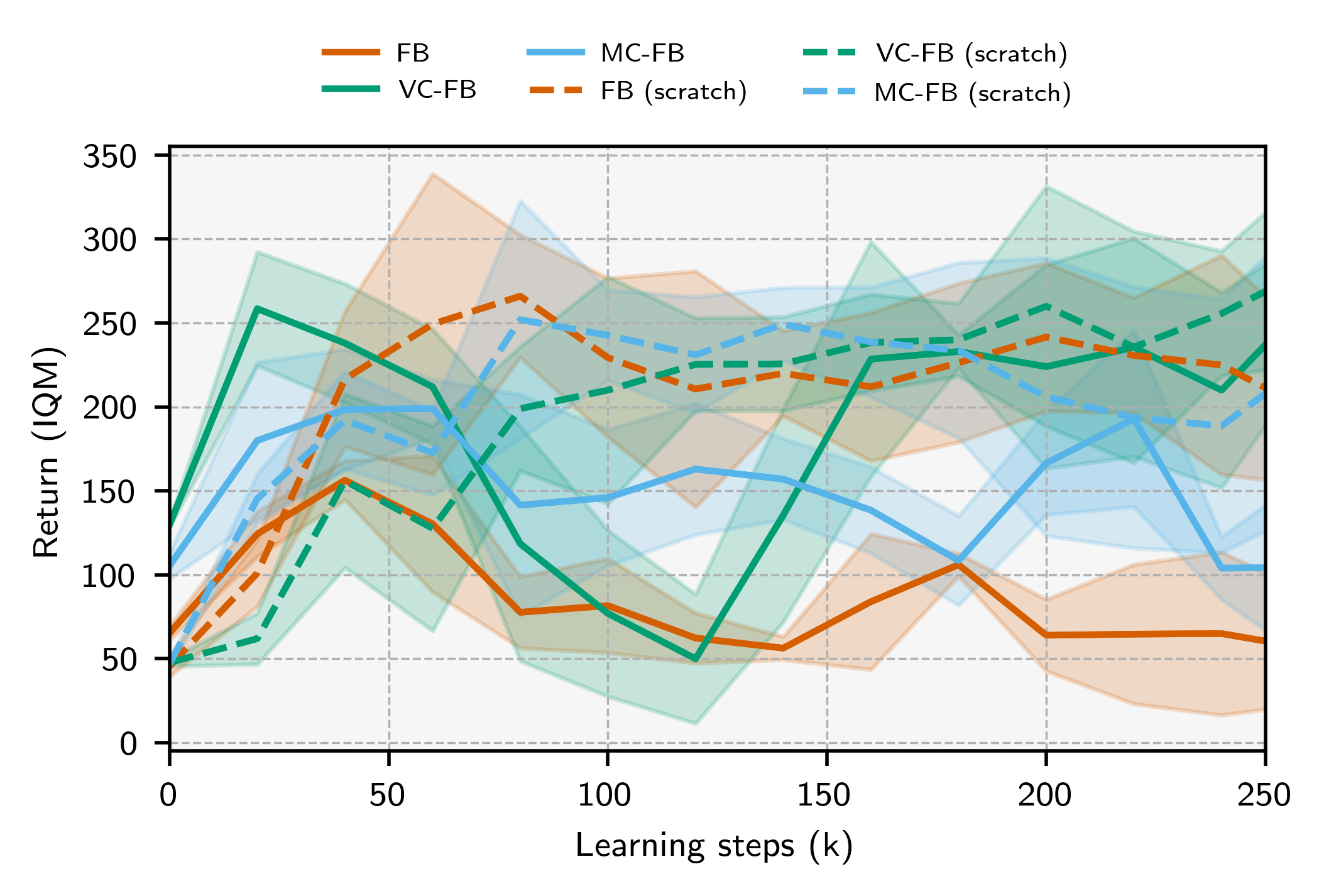
Figure 7: Learning curves for methods finetuned on the full Rnd dataset. Solid lines represent base models trained on Random-100k, then finetuned; dashed lines represent models trained from scratch. The finetuned models perform no better than models trained from scratch after 250k learning steps, suggesting model re-training is currently a better strategy than offline finetuning.

Online finetuning. We considered the online finetuning setup where a trained representation is deployed in the target environment, required to complete a specified task, and allowed to collect a replay buffer of reward-labelled online experience. We followed a standard online RL protocol where a batch of transitions was sampled from the online replay buffer after each environment step for use in updating the model’s parameters. We experimented with fixing $z$ to the target task during in the actor updates (Line 16, Algorithm 1), but found it caused a quick, irrecoverable collapse in actor performance. This suggested uniform samples from $\mathcal{Z}$ provide a form of regularisation. We granted the agents 500k steps of interaction for online finetuning.

We found that performance never improved beyond the pre-trained (init) performance during finetuning. We speculated that this was similar to the well-documented failure mode of online finetuning of CQL (Nakamoto et al., 2023), namely taking sub-optimal actions in the real env, observing unexpectedly high reward, and updating their policy toward these sub-optimal actions. But we note that FB representations do not update w.r.t observed rewards, and so conclude this cannot be the failure mode. Instead it seems likely that FB algorithms cannot use the narrow, unexploratory experience obtained from attempting to perform a specific task to improve model performance.

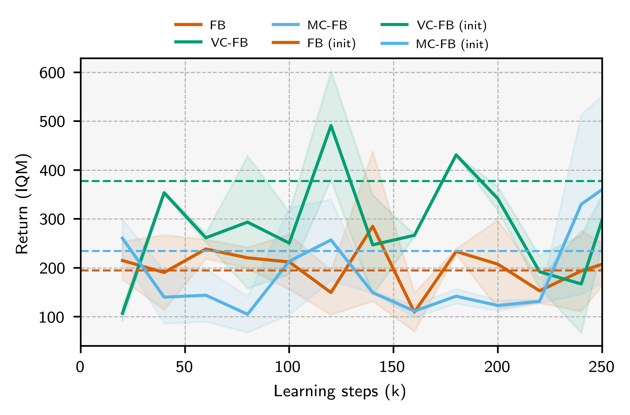
Figure 8: Learning curves for online finetuning. The performance at the end of pre-training (init performance) is plotted as a dashed line for each method. None of the methods consistently outperform their init performance after 250k online transitions.

We believe resolving issues associated with finetuning conservative FB algorithms once the zero-shot requirement is relaxed is an important future direction and hope that details of our negative attempts to this end help facilitate future research.

Appendix E Hyperparameter Sensitivity

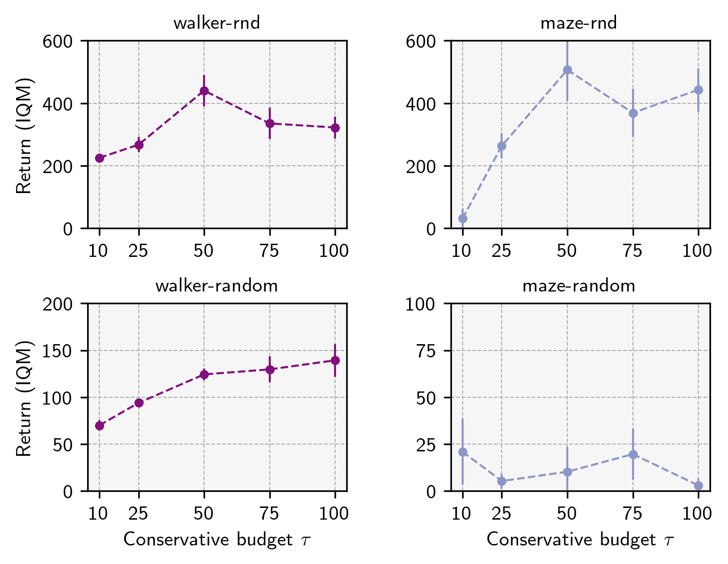
Figure 9: VC-FB sensitivity to conservative budget $\tau$ on Walker and Point-mass Maze. Top: RND dataset; bottom: Random dataset. Maximum IQM return across the training run averaged over 3 random seeds

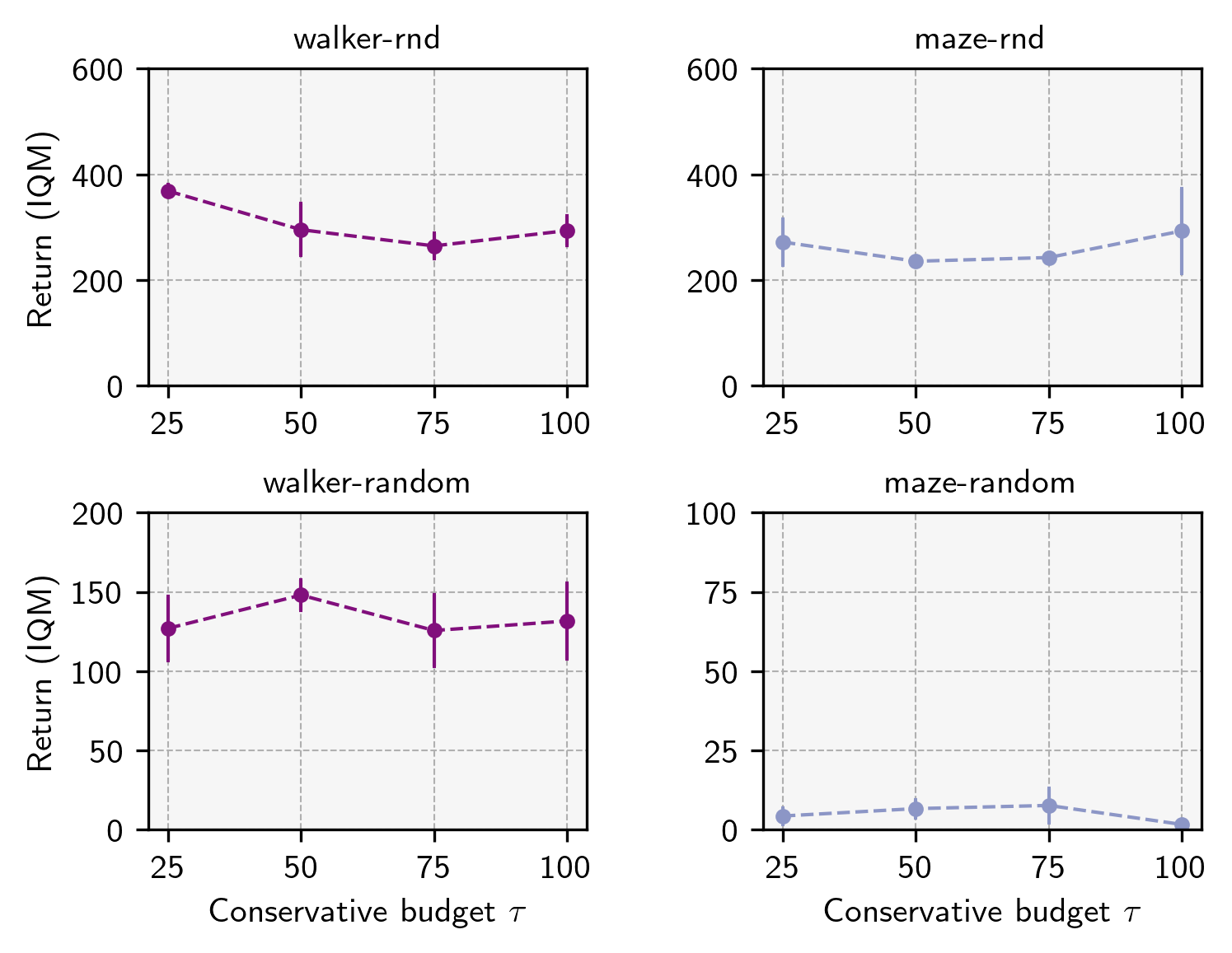
Figure 10: MC-FB sensitivity to conservative budget $\tau$ on Walker and Point-mass Maze. Top: RND dataset; bottom: Random dataset. Maximum IQM return across the training run averaged over 3 random seeds

Appendix F Learning Curves

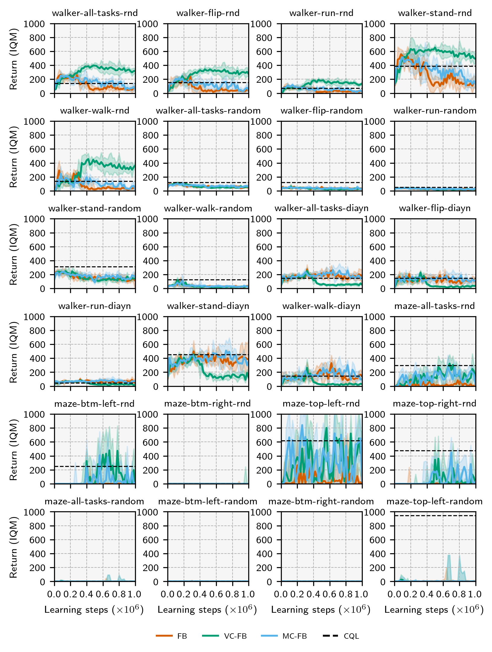
Figure 12: Learning Curves (1/3). Models are evaluated every 20,000 timesteps where we perform 10 rollouts and record the IQM. Curves are the IQM of this value across 5 seeds; shaded areas are one standard deviation.

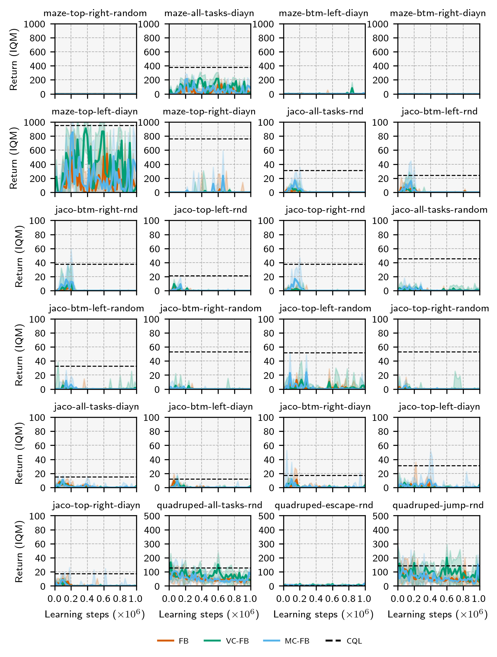
Figure 13: Learning Curves (2/3). Models are evaluated every 20,000 timesteps where we perform 10 rollouts and record the IQM. Curves are the IQM of this value across 5 seeds; shaded areas are one standard deviation.

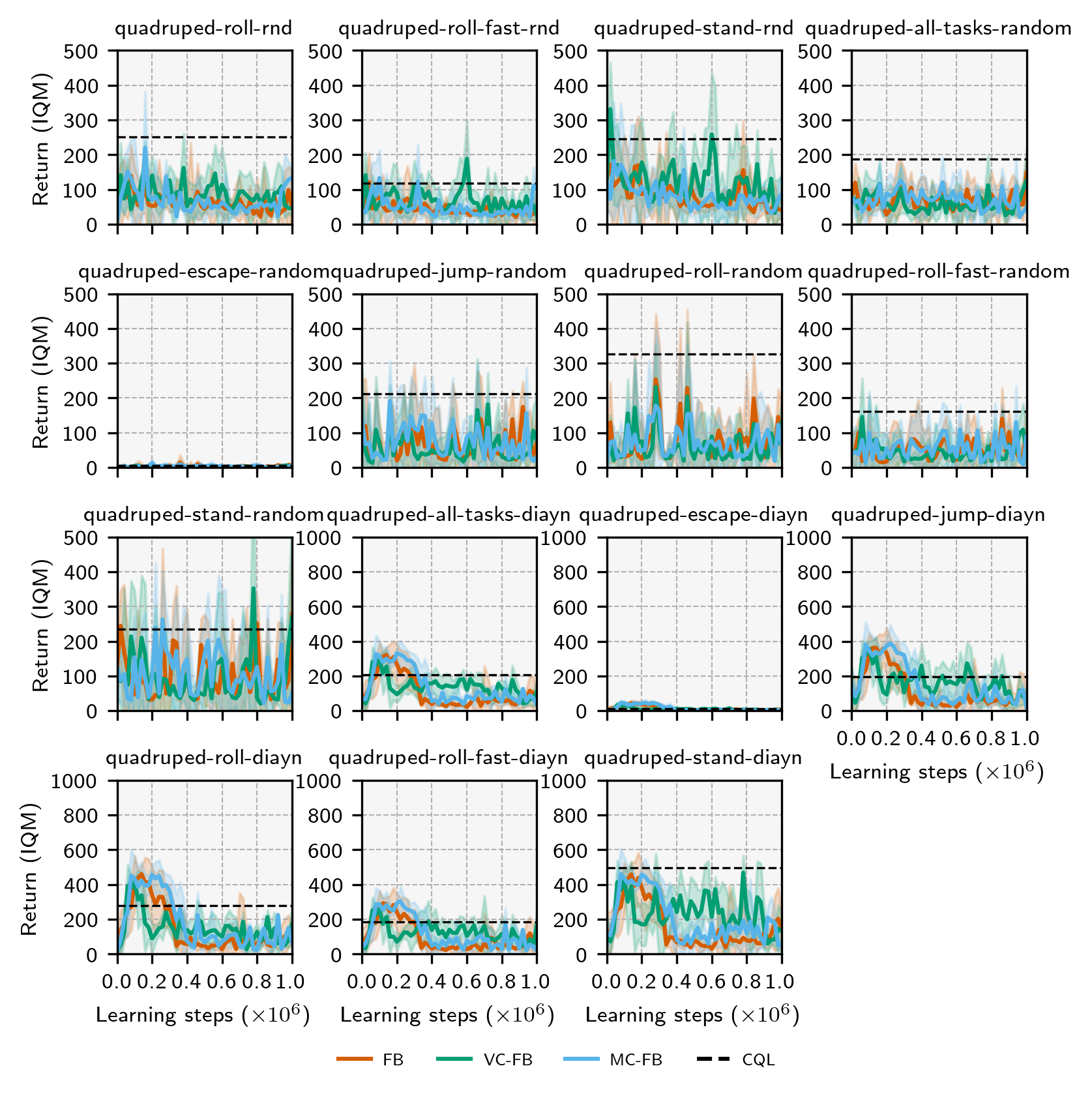
Figure 14: Learning Curves (3/3). Models are evaluated every 20,000 timesteps where we perform 10 rollouts and record the IQM. Curves are the IQM of this value across 5 seeds; shaded areas are one standard deviation.

Appendix G Code Snippets

G.1 Update Step

⬇

1 def update_fb(

2 self,

3 observations: torch.Tensor,

4 actions: torch.Tensor,

5 next_observations: torch.Tensor,

6 discounts: torch.Tensor,

7 zs: torch.Tensor,

8 step: int,

9 ) -> Dict[str, float]:

10 """

11 Calculates the loss for the forward-backward representation network.

12 Loss contains two components:

13 1. Forward-backward representation (core) loss: a Bellman update

14 on the successor measure (equation 24, Appendix B)

15 2. Conservative loss: penalises out-of-distribution actions

16 Args:

17 observations: observation tensor of shape [batch_size, observation_length]

18 actions: action tensor of shape [batch_size, action_length]

19 next_observations: next observation tensor of

20 shape [batch_size, observation_length]

21 discounts: discount tensor of shape [batch_size, 1]

22 zs: policy tensor of shape [batch_size, z_dimension]

23 step: current training step

24 Returns:

25 metrics: dictionary of metrics for logging

26 """

27

28 # update step common to all FB models

29 (

30 core_loss,

31 core_metrics,

32 F1,

33 F2,

34 B_next,

35 M1_next,

36 M2_next,

37 _,

38 _,

39 actor_std_dev,

40 ) = self._update_fb_inner(

41 observations=observations,

42 actions=actions,

43 next_observations=next_observations,

44 discounts=discounts,

45 zs=zs,

46 step=step,

47 )

48

49 # calculate MC or VC penalty

50 if self.mcfb:

51 (

52 conservative_penalty,

53 conservative_metrics,

54 ) = self._measure_conservative_penalty(

55 observations=observations,

56 next_observations=next_observations,

57 zs=zs,

58 actor_std_dev=actor_std_dev,

59 F1=F1,

60 F2=F2,

61 B_next=B_next,

62 M1_next=M1_next,

63 M2_next=M2_next,

64 )

65 # VCFB

66 else:

67 (

68 conservative_penalty,

69 conservative_metrics,

70 ) = self._value_conservative_penalty(

71 observations=observations,

72 next_observations=next_observations,

73 zs=zs,

74 actor_std_dev=actor_std_dev,

75 F1=F1,

76 F2=F2,

77 )

78

79 # tune alpha from conservative penalty

80 alpha, alpha_metrics = self._tune_alpha(

81 conservative_penalty=conservative_penalty

82 )

83 conservative_loss = alpha * conservative_penalty

84

85 total_loss = core_loss + conservative_loss

86

87 # step optimiser

88 self.FB_optimiser.zero_grad(set_to_none=True)

89 total_loss.backward()

90 for param in self.FB.parameters():

91 if param.grad is not None:

92 param.grad.data.clamp_(-1, 1)

93 self.FB_optimiser.step()

94

95 return metrics

G.2 Value-Conservative Penalty

⬇

1def _value_conservative_penalty(

2 self,

3 observations: torch.Tensor,

4 next_observations: torch.Tensor,

5 zs: torch.Tensor,

6 actor_std_dev: torch.Tensor,

7 F1: torch.Tensor,

8 F2: torch.Tensor,

9 ) -> torch.Tensor:

10 """

11 Calculates the value conservative penalty for FB.

12 Args:

13 observations: observation tensor of shape [batch_size, observation_length]

14 next_observations: next observation tensor of shape

15 [batch_size, observation_length]

16 zs: task tensor of shape [batch_size, z_dimension]

17 actor_std_dev: standard deviation of the actor

18 F1: forward embedding no. 1

19 F2: forward embedding no. 2

20 Returns:

21 conservative_penalty: the value conservative penalty

22 """

23

24 with torch.no_grad():

25 # repeat observations, next_observations, zs, and Bs

26 # we fold the action sample dimension into the batch dimension

27 # to allow the tensors to be passed through F and B; we then

28 # reshape the output back to maintain the action sample dimension

29 repeated_observations_ood = observations.repeat(

30 self.ood_action_samples, 1, 1

31 ).reshape(self.ood_action_samples * self.batch_size, -1)

32 repeated_zs_ood = zs.repeat(self.ood_action_samples, 1, 1).reshape(

33 self.ood_action_samples * self.batch_size, -1

34 )

35 ood_actions = torch.empty(

36 size=(self.ood_action_samples * self.batch_size, self.action_length),

37 device=self._device,

38 ).uniform_(-1, 1)

39

40 repeated_observations_actor = observations.repeat(

41 self.actor_action_samples, 1, 1

42 ).reshape(self.actor_action_samples * self.batch_size, -1)

43 repeated_next_observations_actor = next_observations.repeat(

44 self.actor_action_samples, 1, 1

45 ).reshape(self.actor_action_samples * self.batch_size, -1)

46 repeated_zs_actor = zs.repeat(self.actor_action_samples, 1, 1).reshape(

47 self.actor_action_samples * self.batch_size, -1

48 )

49 actor_current_actions, _ = self.actor(

50 repeated_observations_actor,

51 repeated_zs_actor,

52 std=actor_std_dev,

53 sample=True,

54 ) # [actor_action_samples * batch_size, action_length]

55

56 actor_next_actions, _ = self.actor(

57 repeated_next_observations_actor,

58 z=repeated_zs_actor,

59 std=actor_std_dev,

60 sample=True,

61 ) # [actor_action_samples * batch_size, action_length]

62

63 # get Fs

64 ood_F1, ood_F2 = self.FB.forward_representation(

65 repeated_observations_ood, ood_actions, repeated_zs_ood

66 ) # [ood_action_samples * batch_size, latent_dim]

67

68 actor_current_F1, actor_current_F2 = self.FB.forward_representation(

69 repeated_observations_actor, actor_current_actions, repeated_zs_actor

70 ) # [actor_action_samples * batch_size, latent_dim]

71 actor_next_F1, actor_next_F2 = self.FB.forward_representation(

72 repeated_next_observations_actor, actor_next_actions, repeated_zs_actor

73 ) # [actor_action_samples * batch_size, latent_dim]

74 repeated_F1, repeated_F2 = F1.repeat(

75 self.actor_action_samples, 1, 1

76 ).reshape(self.actor_action_samples * self.batch_size, -1), F2.repeat(

77 self.actor_action_samples, 1, 1

78 ).reshape(

79 self.actor_action_samples * self.batch_size, -1

80 )

81 cat_F1 = torch.cat(

82 [

83 ood_F1,

84 actor_current_F1,

85 actor_next_F1,

86 repeated_F1,

87 ],

88 dim=0,

89 )

90 cat_F2 = torch.cat(

91 [

92 ood_F2,

93 actor_current_F2,

94 actor_next_F2,

95 repeated_F2,

96 ],

97 dim=0,

98 )

99

100 repeated_zs = zs.repeat(self.total_action_samples, 1, 1).reshape(

101 self.total_action_samples * self.batch_size, -1

102 )

103

104 # convert to Qs

105 cql_cat_Q1 = torch.einsum("sd, sd -> s", cat_F1, repeated_zs).reshape(

106 self.total_action_samples, self.batch_size, -1

107 )

108 cql_cat_Q2 = torch.einsum("sd, sd -> s", cat_F2, repeated_zs).reshape(

109 self.total_action_samples, self.batch_size, -1

110 )

111

112 cql_logsumexp = (

113 torch.logsumexp(cql_cat_Q1, dim=0).mean()

114 + torch.logsumexp(cql_cat_Q2, dim=0).mean()

115 )

116

117 # get existing Qs

118 Q1, Q2 = [torch.einsum("sd, sd -> s", F, zs) for F in [F1, F2]]

119

120 conservative_penalty = cql_logsumexp - (Q1 + Q2).mean()

121

122 return conservative_penalty

G.3 Measure-Conservative Penalty

⬇

1def _measure_conservative_penalty(

2 self,

3 observations: torch.Tensor,

4 next_observations: torch.Tensor,

5 zs: torch.Tensor,

6 actor_std_dev: torch.Tensor,

7 F1: torch.Tensor,

8 F2: torch.Tensor,

9 B_next: torch.Tensor,

10 M1_next: torch.Tensor,

11 M2_next: torch.Tensor,

12 ) -> torch.Tensor:

13 """

14 Calculates the measure conservative penalty.

15 Args:

16 observations: observation tensor of shape [batch_size, observation_length]

17 next_observations: next observation tensor of shape

18 [batch_size, observation_length]

19 zs: task tensor of shape [batch_size, z_dimension]

20 actor_std_dev: standard deviation of the actor

21 F1: forward embedding no. 1

22 F2: forward embedding no. 2

23 B_next: backward embedding

24 M1_next: successor measure no. 1

25 M2_next: successor measure no. 2

26 Returns:

27 conservative_penalty: the measure conservative penalty

28 """

29

30 with torch.no_grad():

31 # repeat observations, next_observations, zs, and Bs

32 # we fold the action sample dimension into the batch dimension

33 # to allow the tensors to be passed through F and B; we then

34 # reshape the output back to maintain the action sample dimension

35 repeated_observations_ood = observations.repeat(

36 self.ood_action_samples, 1, 1

37 ).reshape(self.ood_action_samples * self.batch_size, -1)

38 repeated_zs_ood = zs.repeat(self.ood_action_samples, 1, 1).reshape(

39 self.ood_action_samples * self.batch_size, -1

40 )

41 ood_actions = torch.empty(

42 size=(self.ood_action_samples * self.batch_size, self.action_length),

43 device=self._device,

44 ).uniform_(-1, 1)

45

46 repeated_observations_actor = observations.repeat(

47 self.actor_action_samples, 1, 1

48 ).reshape(self.actor_action_samples * self.batch_size, -1)

49 repeated_next_observations_actor = next_observations.repeat(

50 self.actor_action_samples, 1, 1

51 ).reshape(self.actor_action_samples * self.batch_size, -1)

52 repeated_zs_actor = zs.repeat(self.actor_action_samples, 1, 1).reshape(

53 self.actor_action_samples * self.batch_size, -1

54 )

55 actor_current_actions, _ = self.actor(

56 repeated_observations_actor,

57 repeated_zs_actor,

58 std=actor_std_dev,

59 sample=True,

60 ) # [actor_action_samples * batch_size, action_length]

61

62 actor_next_actions, _ = self.actor(

63 repeated_next_observations_actor,

64 z=repeated_zs_actor,

65 std=actor_std_dev,

66 sample=True,

67 ) # [actor_action_samples * batch_size, action_length]

68

69 # get Fs

70 ood_F1, ood_F2 = self.FB.forward_representation(

71 repeated_observations_ood, ood_actions, repeated_zs_ood

72 ) # [ood_action_samples * batch_size, latent_dim]

73

74 actor_current_F1, actor_current_F2 = self.FB.forward_representation(

75 repeated_observations_actor, actor_current_actions, repeated_zs_actor

76 ) # [actor_action_samples * batch_size, latent_dim]

77 actor_next_F1, actor_next_F2 = self.FB.forward_representation(

78 repeated_next_observations_actor, actor_next_actions, repeated_zs_actor

79 ) # [actor_action_samples * batch_size, latent_dim]

80 repeated_F1, repeated_F2 = F1.repeat(

81 self.actor_action_samples, 1, 1

82 ).reshape(self.actor_action_samples * self.batch_size, -1), F2.repeat(

83 self.actor_action_samples, 1, 1

84 ).reshape(

85 self.actor_action_samples * self.batch_size, -1

86 )

87 cat_F1 = torch.cat(

88 [

89 ood_F1,

90 actor_current_F1,

91 actor_next_F1,

92 repeated_F1,

93 ],

94 dim=0,

95 )

96 cat_F2 = torch.cat(

97 [

98 ood_F2,

99 actor_current_F2,

100 actor_next_F2,

101 repeated_F2,

102 ],

103 dim=0,

104 )

105

106 cml_cat_M1 = torch.einsum("sd, td -> st", cat_F1, B_next).reshape(

107 self.total_action_samples, self.batch_size, -1

108 )

109 cml_cat_M2 = torch.einsum("sd, td -> st", cat_F2, B_next).reshape(

110 self.total_action_samples, self.batch_size, -1

111 )

112

113 cml_logsumexp = (

114 torch.logsumexp(cml_cat_M1, dim=0).mean()

115 + torch.logsumexp(cml_cat_M2, dim=0).mean()

116 )

117

118 conservative_penalty = cml_logsumexp - (M1_next + M2_next).mean()

119

120 return conservative_penalty

G.4 $\alpha$ Tuning

⬇

1def _tune_alpha(

2 self,

3 conservative_penalty: torch.Tensor,

4 ) -> torch.Tensor:

5 """

6 Tunes the conservative penalty weight (alpha) w.r.t. target penalty.

7 Discussed in Appendix B.1.4

8 Args:

9 conservative_penalty: the current conservative penalty

10 Returns:

11 alpha: the updated alpha

12 """

13

14 # alpha auto-tuning

15 alpha = torch.clamp(self.critic_log_alpha.exp(), min=0.0, max=1e6)

16 alpha_loss = (

17 -0.5 * alpha * (conservative_penalty - self.target_conservative_penalty)

18 )

19

20 self.critic_alpha_optimiser.zero_grad()

21 alpha_loss.backward(retain_graph=True)

22 self.critic_alpha_optimiser.step()

23 alpha = torch.clamp(self.critic_log_alpha.exp(), min=0.0, max=1e6).detach()

24

25 return alpha

References

- Agarwal et al. (2021) Rishabh Agarwal, Max Schwarzer, Pablo Samuel Castro, Aaron C Courville, and Marc Bellemare. Deep reinforcement learning at the edge of the statistical precipice. Advances in neural information processing systems, 34:29304–29320, 2021.
- Ba et al. (2016) Jimmy Lei Ba, Jamie Ryan Kiros, and Geoffrey E Hinton. Layer normalization. arXiv preprint arXiv:1607.06450, 2016.
- Barreto et al. (2017) André Barreto, Will Dabney, Rémi Munos, Jonathan J Hunt, Tom Schaul, Hado P van Hasselt, and David Silver. Successor features for transfer in reinforcement learning. Advances in neural information processing systems, 30, 2017.
- Bellman (1957) Richard Bellman. A markovian decision process. Journal of mathematics and mechanics, pp. 679–684, 1957.
- Blier et al. (2021) Léonard Blier, Corentin Tallec, and Yann Ollivier. Learning successor states and goal-dependent values: A mathematical viewpoint. arXiv preprint arXiv:2101.07123, 2021.
- Borsa et al. (2018) Diana Borsa, André Barreto, John Quan, Daniel Mankowitz, Rémi Munos, Hado Van Hasselt, David Silver, and Tom Schaul. Universal successor features approximators. arXiv preprint arXiv:1812.07626, 2018.
- Burda et al. (2018) Yuri Burda, Harrison Edwards, Amos Storkey, and Oleg Klimov. Exploration by random network distillation. arXiv preprint arXiv:1810.12894, 2018.
- Chua et al. (2018) Kurtland Chua, Roberto Calandra, Rowan McAllister, and Sergey Levine. Deep reinforcement learning in a handful of trials using probabilistic dynamics models. In Proceedings of the 32nd International Conference on Neural Information Processing Systems, NIPS’18, pp. 4759–4770, 2018.
- Dayan (1993) Peter Dayan. Improving generalization for temporal difference learning: The successor representation. Neural computation, 5(4):613–624, 1993.
- Deisenroth & Rasmussen (2011) Marc Deisenroth and Carl E Rasmussen. Pilco: A model-based and data-efficient approach to policy search. In Proceedings of the 28th International Conference on machine learning (ICML-11), pp. 465–472, 2011.
- Efron (1992) Bradley Efron. Bootstrap methods: another look at the jackknife. In Breakthroughs in statistics: Methodology and distribution, pp. 569–593. Springer, 1992.
- Eysenbach et al. (2018) Benjamin Eysenbach, Abhishek Gupta, Julian Ibarz, and Sergey Levine. Diversity is all you need: Learning skills without a reward function. arXiv preprint arXiv:1802.06070, 2018.
- Fu et al. (2020) Justin Fu, Aviral Kumar, Ofir Nachum, George Tucker, and Sergey Levine. D4rl: Datasets for deep data-driven reinforcement learning. arXiv preprint arXiv:2004.07219, 2020.
- Fujimoto et al. (2019) Scott Fujimoto, David Meger, and Doina Precup. Off-policy deep reinforcement learning without exploration. In International conference on machine learning, pp. 2052–2062. PMLR, 2019.
- Ghosh et al. (2023) Dibya Ghosh, Chethan Anand Bhateja, and Sergey Levine. Reinforcement learning from passive data via latent intentions. In International Conference on Machine Learning, pp. 11321–11339. PMLR, 2023.
- Ha & Schmidhuber (2018) David Ha and Jürgen Schmidhuber. World models. arXiv preprint arXiv:1803.10122, 2018.
- Haarnoja et al. (2018) Tuomas Haarnoja, Aurick Zhou, Pieter Abbeel, and Sergey Levine. Soft actor-critic: Off-policy maximum entropy deep reinforcement learning with a stochastic actor. In International conference on machine learning, pp. 1861–1870, 2018.
- Hafner et al. (2019) Danijar Hafner, Timothy Lillicrap, Jimmy Ba, and Mohammad Norouzi. Dream to control: Learning behaviors by latent imagination. arXiv preprint arXiv:1912.01603, 2019.
- Hafner et al. (2023) Danijar Hafner, Jurgis Pasukonis, Jimmy Ba, and Timothy Lillicrap. Mastering diverse domains through world models. arXiv preprint arXiv:2301.04104, 2023.
- Jaderberg et al. (2016) Max Jaderberg, Volodymyr Mnih, Wojciech Marian Czarnecki, Tom Schaul, Joel Z Leibo, David Silver, and Koray Kavukcuoglu. Reinforcement learning with unsupervised auxiliary tasks. arXiv preprint arXiv:1611.05397, 2016.
- Kidambi et al. (2020) Rahul Kidambi, Aravind Rajeswaran, Praneeth Netrapalli, and Thorsten Joachims. Morel: Model-based offline reinforcement learning. Advances in neural information processing systems, 33:21810–21823, 2020.
- Kirk et al. (2023) Robert Kirk, Amy Zhang, Edward Grefenstette, and Tim Rocktäschel. A survey of zero-shot generalisation in deep reinforcement learning. Journal of Artificial Intelligence Research, 76:201–264, 2023.
- Kumar et al. (2019) Aviral Kumar, Justin Fu, Matthew Soh, George Tucker, and Sergey Levine. Stabilizing off-policy q-learning via bootstrapping error reduction. In H. Wallach, H. Larochelle, A. Beygelzimer, F. d'Alché-Buc, E. Fox, and R. Garnett (eds.), Advances in Neural Information Processing Systems, volume 32. Curran Associates, Inc., 2019. URL https://proceedings.neurips.cc/paper_files/paper/2019/file/c2073ffa77b5357a498057413bb09d3a-Paper.pdf.
- Kumar et al. (2020) Aviral Kumar, Aurick Zhou, George Tucker, and Sergey Levine. Conservative q-learning for offline reinforcement learning. arXiv preprint arXiv:2006.04779, 2020.
- Kumar et al. (2022) Aviral Kumar, Rishabh Agarwal, Xinyang Geng, George Tucker, and Sergey Levine. Offline q-learning on diverse multi-task data both scales and generalizes. arXiv preprint arXiv:2211.15144, 2022.
- Lazaric (2012) Alessandro Lazaric. Transfer in reinforcement learning: a framework and a survey. In Reinforcement Learning: State-of-the-Art, pp. 143–173. Springer, 2012.
- Levine et al. (2020) Sergey Levine, Aviral Kumar, George Tucker, and Justin Fu. Offline reinforcement learning: Tutorial, review, and perspectives on open problems. arXiv preprint arXiv:2005.01643, 2020.
- Lillicrap et al. (2016) Timothy P. Lillicrap, Jonathan J. Hunt, Alexander Pritzel, Nicolas Heess, Tom Erez, Yuval Tassa, David Silver, and Daan Wierstra. Continuous control with deep reinforcement learning. In ICLR (Poster), 2016. URL http://arxiv.org/abs/1509.02971.
- Lyu et al. (2022) Jiafei Lyu, Xiaoteng Ma, Xiu Li, and Zongqing Lu. Mildly conservative q-learning for offline reinforcement learning. Advances in Neural Information Processing Systems, 35:1711–1724, 2022.
- Nakamoto et al. (2023) Mitsuhiko Nakamoto, Yuexiang Zhai, Anikait Singh, Max Sobol Mark, Yi Ma, Chelsea Finn, Aviral Kumar, and Sergey Levine. Cal-ql: Calibrated offline rl pre-training for efficient online fine-tuning. arXiv preprint arXiv:2303.05479, 2023.
- Samuel (1959) Arthur L Samuel. Some studies in machine learning using the game of checkers. IBM Journal of research and development, 3(3):210–229, 1959.
- Schaul et al. (2015) Tom Schaul, Daniel Horgan, Karol Gregor, and David Silver. Universal value function approximators. In International conference on machine learning, pp. 1312–1320. PMLR, 2015.
- Schrittwieser et al. (2020) Julian Schrittwieser, Ioannis Antonoglou, Thomas Hubert, Karen Simonyan, Laurent Sifre, Simon Schmitt, Arthur Guez, Edward Lockhart, Demis Hassabis, Thore Graepel, et al. Mastering atari, go, chess and shogi by planning with a learned model. Nature, 588(7839):604–609, 2020.
- Sekar et al. (2020) Ramanan Sekar, Oleh Rybkin, Kostas Daniilidis, Pieter Abbeel, Danijar Hafner, and Deepak Pathak. Planning to explore via self-supervised world models. In International Conference on Machine Learning, pp. 8583–8592. PMLR, 2020.
- Sutton & Barto (2018) Richard Sutton and Andrew Barto. Reinforcement Learning: An Introduction. The MIT Press, second edition, 2018.
- Sutton (1988) Richard S Sutton. Learning to predict by the methods of temporal differences. Machine learning, 3:9–44, 1988.
- Sutton (1991) Richard S Sutton. Dyna, an integrated architecture for learning, planning, and reacting. ACM Sigart Bulletin, 2(4):160–163, 1991.
- Tassa et al. (2018) Yuval Tassa, Yotam Doron, Alistair Muldal, Tom Erez, Yazhe Li, Diego de Las Casas, David Budden, Abbas Abdolmaleki, Josh Merel, Andrew Lefrancq, et al. Deepmind control suite. arXiv preprint arXiv:1801.00690, 2018.
- Touati & Ollivier (2021) Ahmed Touati and Yann Ollivier. Learning one representation to optimize all rewards. Advances in Neural Information Processing Systems, 34:13–23, 2021.
- Touati et al. (2022) Ahmed Touati, Jérémy Rapin, and Yann Ollivier. Does zero-shot reinforcement learning exist? In The Eleventh International Conference on Learning Representations, 2022.
- Yarats et al. (2022) Denis Yarats, David Brandfonbrener, Hao Liu, Michael Laskin, Pieter Abbeel, Alessandro Lazaric, and Lerrel Pinto. Don’t change the algorithm, change the data: Exploratory data for offline reinforcement learning. arXiv preprint arXiv:2201.13425, 2022.
- Yu et al. (2020) Tianhe Yu, Garrett Thomas, Lantao Yu, Stefano Ermon, James Y Zou, Sergey Levine, Chelsea Finn, and Tengyu Ma. Mopo: Model-based offline policy optimization. Advances in Neural Information Processing Systems, 33:14129–14142, 2020.